Obtaining Summary Statistics with SPSS

Math 260

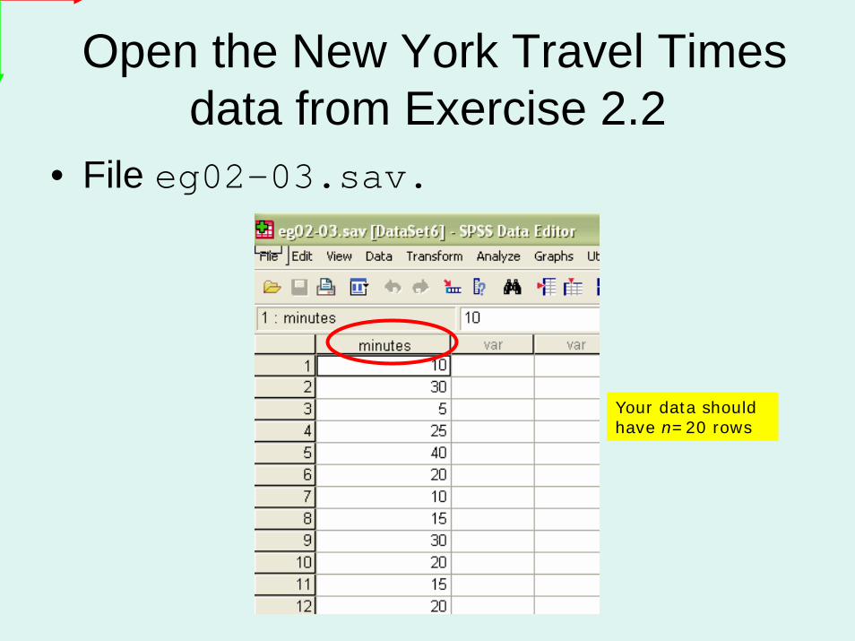
Open the New York Travel Times data from Exercise 2.2

• File eg02-03.sav.

Your data should have n=20 rows

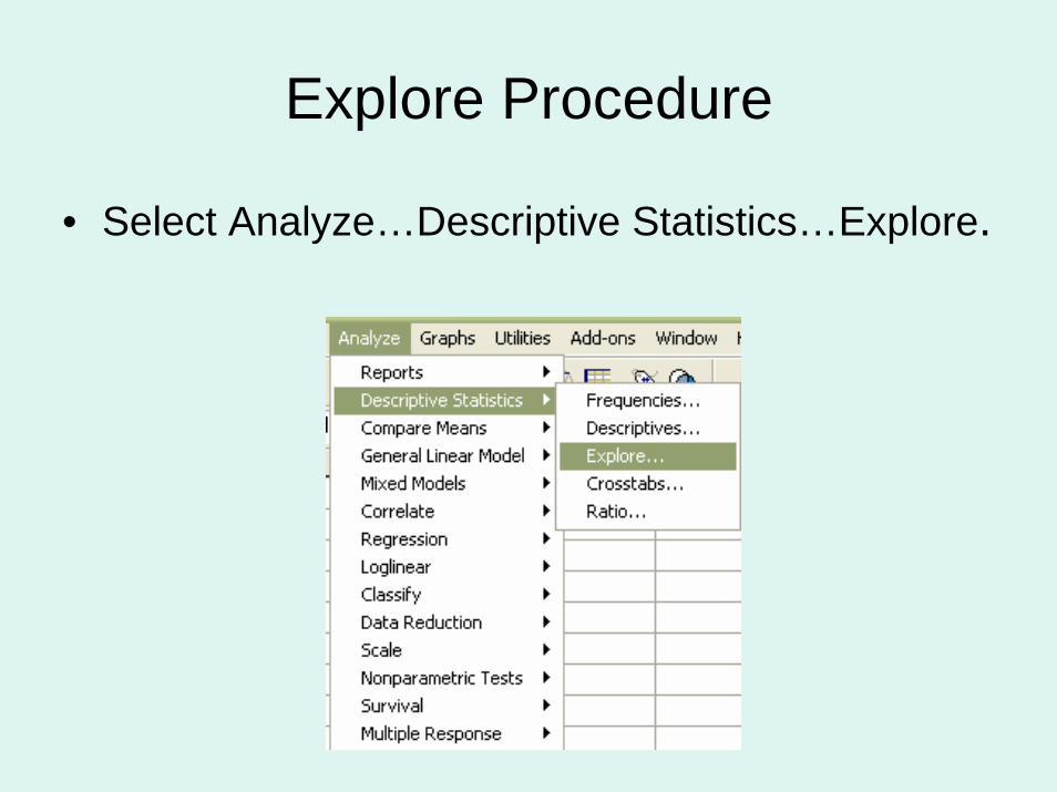
Explore Procedure

• Select Analyze…Descriptive Statistics…Explore.

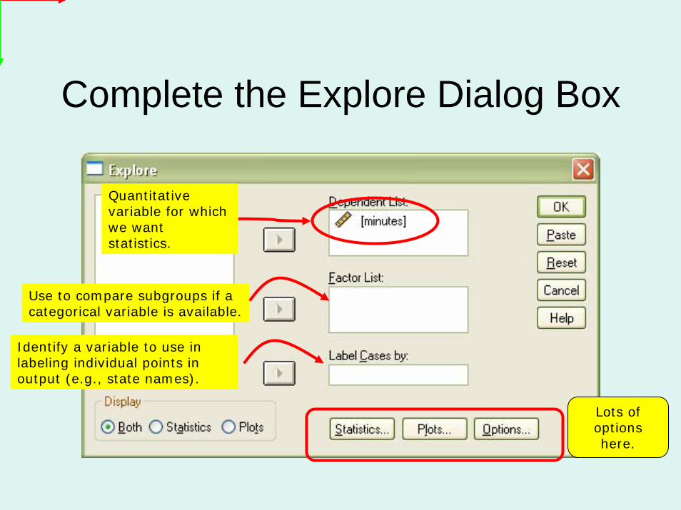
Complete the Explore Dialog Box

Quantitative variable for which we want statistics.

Use to compare subgroups if a categorical variable is available.

Lots of options here.

Identify a variable to use in labeling individual points in output (e.g., state names).

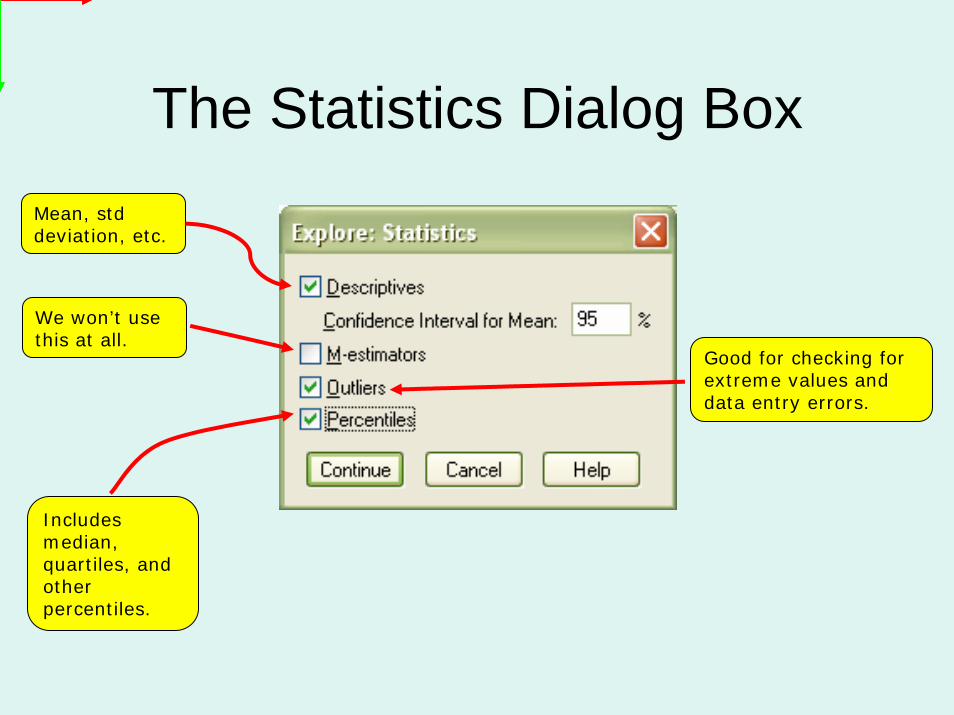
The Statistics Dialog BoxMean, std deviation, etc.

We won’t use this at all.

Good for checking for extreme values and data entry errors.

Includes median, quartiles, and other percentiles.

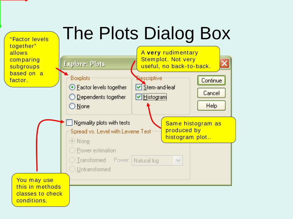
The Plots Dialog Box“Factor levels together”allows comparing subgroups based on a factor.

You may use this in methods classes to check conditions.

A very rudimentary Stemplot. Not very useful, no back-to-back.

Same histogram as produced by histogram plot..

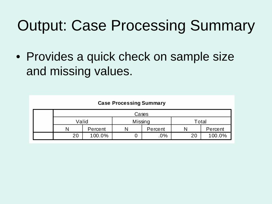
Output: Case Processing Summary

• Provides a quick check on sample size and missing values.

Case Processing Summary

20 100.0% 0 .0% 20 100.0% N Percent N Percent N Percent

Valid Missing TotalCases

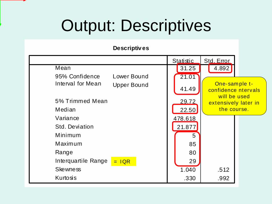
Output: DescriptivesDescriptives

31.25 4.89221.01

41.49

29.7222.50

478.61821.877

5858029

1.040 .512.330 .992

MeanLower BoundUpper Bound

95% ConfidenceInterval for Mean

5% Trimmed MeanMedianVarianceStd. DeviationMinimumMaximumRangeInterquarti le RangeSkewnessKurtosis

Statistic Std. Error

One-sample t-confidence ntervals

will be used extensively later in

the course.

= IQR

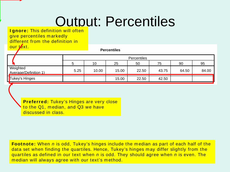
Percentiles

5.25 10.00 15.00 22.50 43.75 64.50 84.00

15.00 22.50 42.50

WeightedAverage(Definition 1)Tukey's Hinges

5 10 25 50 75 90 95Percentiles

Output: Percentiles

Preferred: Tukey’s Hinges are very close to the Q1, median, and Q3 we have discussed in class.

Ignore: This definition will often give percentiles markedly different from the definition in our text.

Footnote: When n is odd, Tukey’s hinges include the median as part of each half of the data set when finding the quartiles. Hence, Tukey’s hinges may differ slightly from the quartiles as defined in our text when n is odd. They should agree when n is even. The median will always agree with our text’s method.

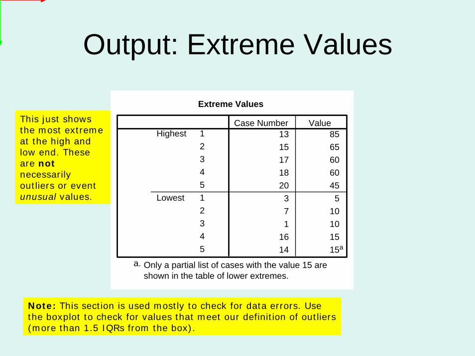
Output: Extreme Values

Extreme Values

13 8515 6517 6018 6020 45

3 57 101 10

16 1514 15a

1234512345

Highest

Lowest

Case Number Value

Only a partial list of cases with the value 15 areshown in the table of lower extremes.

a.

This just shows the most extreme at the high and low end. These are notnecessarily outliers or event unusual values.

Note: This section is used mostly to check for data errors. Use the boxplot to check for values that meet our definition of outliers (more than 1.5 IQRs from the box).

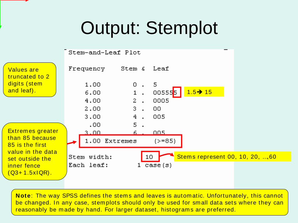
Output: Stemplot

1.5 15

Stems represent 00, 10, 20, …,60

Values are truncated to 2 digits (stem and leaf).

Extremes greater than 85 because 85 is the first value in the data set outside the inner fence (Q3+1.5xIQR).

Note: The way SPSS defines the stems and leaves is automatic. Unfortunately, this cannot be changed. In any case, stemplots should only be used for small data sets where they can reasonably be made by hand. For larger dataset, histograms are preferred.

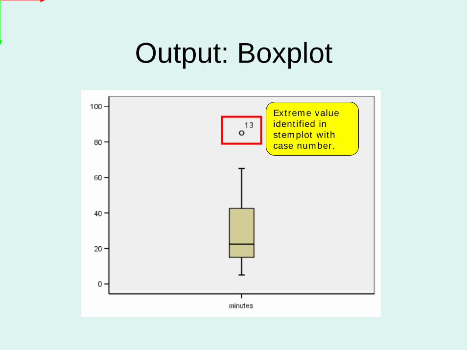
Output: Boxplot

Extreme value identified in stemplot with case number.

Notes

• Histogram output is not shown here as it was discussed in the Intro to SPSS help sheet.

• Another example follows to illustrate subgroup analysis.

• Open the cars.sav file again and explore weights by country of origin.

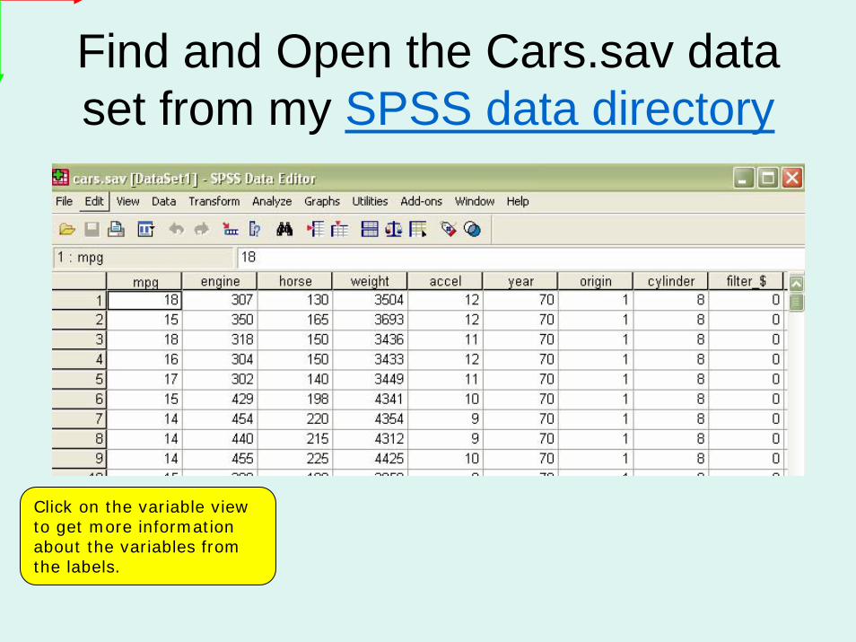
Find and Open the Cars.sav data set from my SPSS data directory

Click on the variable view to get more information about the variables from the labels.

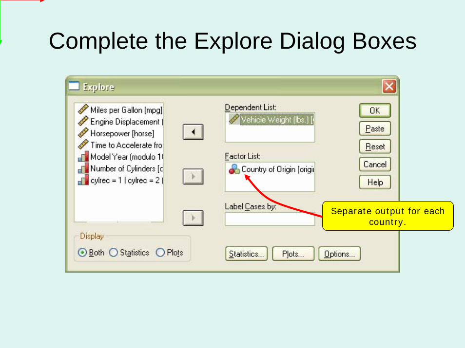
Complete the Explore Dialog Boxes

Separate output for each country.

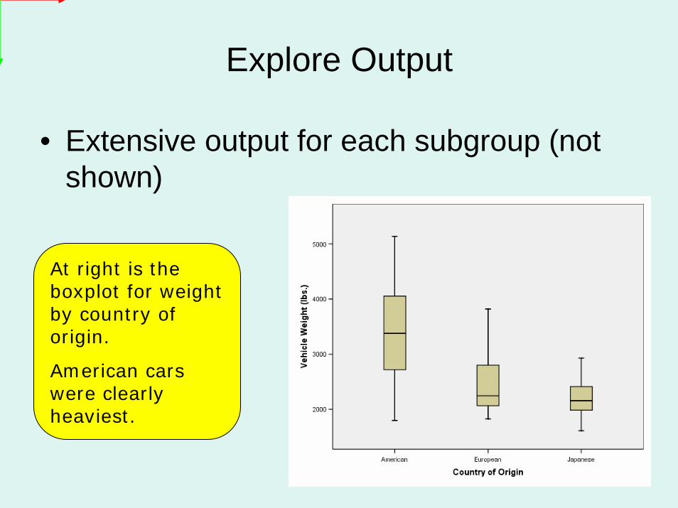
Explore Output

• Extensive output for each subgroup (not shown)

At right is the boxplot for weight by country of origin.

American cars were clearly heaviest.

Other Procedures

• Analyze…Descriptive Statistics has other useful procedures for summary statistics:– Descriptives: extensive statistics if no subgroups or

plots are needed.– Frequencies: frequency table and statistics, especially

for discrete data (small number of possible values).• Analyze…Compare Means…Means is also good

for a concise summary of subgroups.• Experiment and see what you prefer! • Ask questions if you have problems.