Ocean Circulation under Globally Glaciated Snowball … · Ocean Circulation under Globally Glaciated Snowball Earth Conditions: Steady-State Solutions YOSEF ASHKENAZY Department

Ocean Circulation under Globally Glaciated Snowball Earth Conditions:Steady-State Solutions

YOSEF ASHKENAZY

Department of Solar Energy and Environmental Physics, BIDR, Ben-Gurion University, Midreshet Ben-Gurion, Israel

HEZI GILDOR

The Fredy and Nadine Herrmann Institute of Earth Sciences, The Hebrew University of Jerusalem, Jerusalem, Israel

MARTIN LOSCH

Alfred-Wegener-Institut, Helmholtz-Zentrum f€ur Polar- und Meeresforschung, Bremerhaven, Germany

ELI TZIPERMAN

Department of Earth and Planetary Sciences and School of Engineering and Applied Sciences, Harvard University,

Cambridge, Massachusetts

(Manuscript received 15 April 2013, in final form 27 August 2013)

ABSTRACT

Between ;750 and 635 million years ago, during the Neoproterozoic era, the earth experienced at least

two significant, possibly global, glaciations, termed ‘‘Snowball Earth.’’ While many studies have focused on

the dynamics and the role of the atmosphere and ice flow over the ocean in these events, only a few have

investigated the related associated ocean circulation, and no study has examined the ocean circulation under

a thick (;1 km deep) sea ice cover, driven by geothermal heat flux. Here, a thick sea ice–flow model coupled

to an ocean general circulation model is used to study the ocean circulation under Snowball Earth conditions.

The ocean circulation is first investigated under a simplified zonal symmetry assumption, and (i) strong

equatorial zonal jets and (ii) a strongmeridional overturning cell are found, limited to an area very close to the

equator. The authors derive an analytic approximation for the latitude–depth ocean dynamics and find that

the extent of the meridional overturning circulation cell only depends on the horizontal eddy viscosity and b

(the change of the Coriolis parameter with latitude). The analytic approximation closely reproduces the

numerical results. Three-dimensional ocean simulations, with reconstructed Neoproterozoic continental

configuration, confirm the zonally symmetric dynamics and show additional boundary currents and strong

upwelling and downwelling near the continents.

1. Introduction

The Neoproterozoic ‘‘Snowball’’ events are perhaps

the most drastic climate events in earth’s history. Be-

tween 750 and 580 million years ago (Ma), the earth

experienced at least two major, possibly global, glacia-

tions (e.g., Harland 1964; Kirschvink 1992; Hoffman and

Schrag 2002; Macdonald et al. 2010; Evans and Raub

2011). During these events (the Sturian and Marinoan

ice ages), ice extended to low latitudes over both ocean

and land. It is still debated whether the ocean was en-

tirely covered by thick ice (‘‘hard Snowball’’) (e.g.,

Allen and Etienne 2008; Pierrehumbert et al. 2011),

perhaps except very limited regions of sea ice–free ocean,

such as around volcanic islands (Schrag and Hoffman

2001) (that could have provided a refuge for photosyn-

thetic life during these periods), or whether the tropical

ocean was partially ice free or perhaps covered by thin

ice (‘‘soft Snowball‘‘) (e.g., Yang et al. 2012c).

The initiation, maintenance, and termination of such

a climatic condition pose a first-order problem in ocean

Corresponding author address: Yosef Ashkenazy, Department

of Solar Energy and Environmental Physics, BIDR, Ben-Gurion

University, Midreshet Ben-Gurion, 84990, Israel.

E-mail: [email protected]

24 JOURNAL OF PHYS ICAL OCEANOGRAPHY VOLUME 44

DOI: 10.1175/JPO-D-13-086.1

� 2014 American Meteorological Society

mailto:[email protected]

and climate dynamics. One may argue that the Snowball

state was predicted by simple energy balance models

(EBMs) (Budyko 1969; Sellers 1969). Snowball dynam-

ics also provide a test case for our understanding of

the climate system as manifested in climate models.

Therefore, in recent years, these questions have been the

focus of numerous studies and attempts to simulate these

climate states using models with different levels of

complexity. The role and dynamics of atmospheric cir-

culation and heat transport, CO2 concentration, cloud

feedbacks, and continental configuration have been stud-

ied (Pierrehumbert 2005; Le Hir et al. 2010; Donnadieu

et al. 2004a; Pierrehumbert 2002, 2004; LeHir et al. 2007).

Recently, the effect of clouds, as well as the role of

atmospheric and oceanic heat transports in the initia-

tion of Snowball Earth events has been studied; these

studies were based on coupled atmosphere–ocean GCMs

and used different setups and configurations including

different CO2 concentrations, different continental con-

figurations, and different sea ice dynamics (Voigt and

Marotzke 2010; Voigt et al. 2011; Yang et al. 2012a,b,c;

Voigt and Abbot 2012). It was concluded that sea ice

dynamics has an important role in the initiation of

Snowball events (Voigt andAbbot 2012). Additionally,

perceived difficulties in exiting a Snowball state by a

CO2 increase alone motivated the study of the role of

dust and clouds over the Snowball ice cover (Abbot

and Pierrehumbert 2010; Le Hir et al. 2010; Abbot and

Halevy 2010; Li and Pierrehumbert 2011; Abbot et al.

2012).

A simple scaling calculation of balancing geothermal

heat input into the ocean with heat escaping through

the ice by diffusion leads to an estimated ice thickness

of 1 km. The ice cover is expected to slowly deform and

flow toward the equator to balance for sublimation (and

melting at the bottom of the ice) at low latitudes and

snow accumulation (and ice freezing at the bottom of

the ice) at high latitudes. The flow and other properties

of such thick ice over a Snowball ocean [‘‘sea glaciers,’’

Warren et al. (2002)] were examined in quite a few re-

cent studies (Goodman and Pierrehumbert 2003;

McKay 2000; Warren et al. 2002; Pollard and Kasting

2005; Campbell et al. 2011; Tziperman et al. 2012;

Pollard and Kasting 2006; Warren and Brandt 2006;

Goodman 2006; Lewis et al. 2007). Snowball Earth

global ice cover is an extreme example within a range of

multiple ice-cover equilibrium states, which have been

studied in a range of simple and complex models (e.g.,

Langen and Alexeev 2004; Rose and Marshall 2009;

Ferreira et al. 2011). In contrast to these many studies of

different climate components during Snowball events,

the ocean circulation during these events has received

little attention. Most model studies of a Snowball climate

used an oceanmixed layermodel only (Baum andCrowley

2001; Crowley and Baum 1993; Baum and Crowley 2003;

Hyde et al. 2000; Jenkins and Smith 1999; Chandler and

Sohl 2000; Poulsen et al. 2001; Romanova et al. 2006;

Donnadieu et al. 2004b; Micheels and Montenari 2008).

The studies that used full ocean general circulation models

(GCMs) concentrated on the ocean’s role in Snowball

initiation and aftermath (Poulsen et al. 2001; Poulsen and

Jacob 2004; Poulsen et al. 2002; Sohl andChandler 2007) or

other aspects of Snowball dynamics in the presence of

oceanic feedback (Voigt et al. 2011; Le Hir et al. 2007;

Yang et al. 2012c; Ferreira et al. 2011;Marotzke andBotzet

2007; Lewis et al. 2007; Voigt and Marotzke 2010; Abbot

et al. 2011; Lewis et al. 2003, 2004). Yet none of these

studies employing ocean GCMs accounted for the

combined effects of thick ice-cover flow and driving by

geothermal heating. Ferreira et al. (2011) simulated an

ocean under a moderately thick (200m) ice cover with

no geothermal heat flux, and calculated a non-steady-

state solution with near-uniform temperature and salin-

ity. They described a vanishing Eulerian circulation

together with strongly parameterized eddy-induced

high-latitude circulation cells.

With both the initiation (Kirschvink 1992; Schrag

et al. 2002; Tziperman et al. 2011) and termination

(Pierrehumbert 2004) of Snowball events still not well

understood, and the question of hard versus soft Snow-

ball still unresolved (Pierrehumbert et al. 2011), our

focus here is the steady-state ocean circulation under

a thick ice cover (hard Snowball). By examining ocean

dynamics under such an extreme climatic state, we aim

to better understand the relevant climate dynamics, and

perhaps even provide constraints on the issues regarding

soft versus hard Snowball states.

To study the 3D ocean dynamics under a thick ice cover,

it is necessary to have a two-dimensional (longitude–

latitude) ice-flow model, and this was recently devel-

oped by Tziperman et al. (2012), based on the ice-shelf

equations of Morland (1987) and MacAyeal (1997),

extending the 1Dmodel of Goodman and Pierrehumbert

(2003). This model is coupled here to the Massachusetts

Institute of Technology General Circulation Model

(MITgcm) (Marshall et al. 1997). Another challenge in

studying the 3D ocean dynamics under a thick ice cover

is that thick ice with lateral variations of hundreds of

meters (as under Snowball conditions) poses a numer-

ical challenge as standard ocean models cannot handle

ice that extends through several vertical layers; we use

the ice-shelf model of Losch (2008), which allows for

this. An alternative, vertically scaled coordinates, was

used by Ferreira et al. (2011).

This paper expands on results briefly reported in

Ashkenazy et al. (2013, hereafter AGLMST), and we

JANUARY 2014 A SHKENAZY ET AL . 25

report the details of the steady-state ocean dynamics

under a thick ice (Snowball) cover, analytically and

numerically, when both geothermal heating and a thick

ice flow are taken into account. We find the ocean cir-

culation to be quite far from the stagnant pool envi-

sioned in some early studies and very different from that

in any other period in the earth’s history. In particular,

the stratification is very weak, as might be expected

(Ferreira et al. 2011), and is dominated by salinity

gradients due to melting and freezing of ice; we find

a meridional overturning circulation that is confined to

the equatorial region, significant zonal equatorial jets,

and strong equatorial meridional overturning circula-

tion (MOC).

The paper is organized as follows. We first describe

the models and configurations used in this study (sec-

tion 2). Then we present the results of the latitude–

depth ocean model coupled to a 1D (latitude) ice-flow

model when geothermal heating is taken into account

(section 3). Analytically approximated solutions of the

2D latitude–depth ocean model are then presented

(section 4). Section 5 presents sensitivity runs to study

the robustness of both numerical results and analytical

approximations, followed by the steady-state results of

a 3D ocean model coupled to a longitude–latitude 2D

ice-flow model in section 6. The results are discussed

and summarized in section 7.

2. Model description

a. Ice-flow model

The ice-flow model solves for the ice depth and ve-

locity over an ocean, as a function of longitude and

latitude, in the presence of continents (Tziperman et al.

2012). The model extends the 1D model of Goodman

and Pierrehumbert (2003), which was based on the

Weertman (1957) formula for ice-shelf deformation.

Because this specific formulation cannot be extended to

ice flows in two horizontal dimensions, we instead used

the ice-shelf approximation (Morland 1987; MacAyeal

1997), which can be extended to two dimensions. The

ice-shelf approximation implies a depth-independent

ice velocity and, in addition, the vertical temperature

profile within the ice is assumed to be linear (Goodman

and Pierrehumbert 2003). The temperature at the upper

ice surface and surface ice sublimation and snow ac-

cumulation are prescribed from the energy balance of

Pollard and Kasting (2005) and are assumed to be con-

stant in time. The temperature and melting/freezing rates

at the bottom of the ice are calculated by the ocean

model. The model’s spatial resolution is set to that of the

ocean, and the model is run in either 1D (latitude only)

or 2D configurations, depending on the ocean model

used; it is typically 18–28.

b. The ocean model—MITgcm

We used the Massachusetts Institute of Technology

General CirculationModel (Marshall et al. 1997), a free-

surface, primitive equation ocean model that uses z co-

ordinates with partial cells in the vertical axis; we use

a longitude–latitude grid. To account for the thick ice,

we used the ice-shelf package of the MITgcm (Losch

2008) that allows ice thicknesses spanning many verti-

cal layers. Parameter values followed Losch (2008).

The ocean was forced at the bottom with a spatially

variable (but constant in time) geothermal heat flux. The

equation of state used here (Jackett and McDougall

1995) was tuned for the present-day ocean, while the

temperature and salinity that we used to simulate Snow-

ball conditions were somewhat outside this range. Sensi-

tivity tests, using mean present-day salinity and mean

salinity that is two times larger than the present-day

value, showed no sensitivity of the results for the cir-

culation. The ocean model was run at two different

configurations, including a zonally symmetric 2D con-

figuration and a near-global 3D configuration, described

as follows.

1) LATITUDE–DEPTH CONFIGURATION

In the 2D runs, the spatial resolution was 18 with 32

vertical levels spanning a depth of 3000m, with vertical

level thicknesses, in meters from top to bottom, of 920,

15 levels 3 10, 12, 17, 23, 32, 45, 61, 82, 110, 148, and

7 levels 3 200; the uppermost level was entirely within

the ice. The steady-state ice thickness was calculated by

the ice model to be approximately 1 km with lateral

variations of less than 100m. The latitudinal extent of

the 2D configuration was from 848S to 848N with walls

specified at these boundaries to avoid having to deal

with the polar singularity of the spherical coordinates.

The bathymetry was either flat or had a Gaussian ridge

centered at f0 with a height of h0 5 1500m and widthffiffiffi2

ps5 78:

h(f)5 h0e2(f2f

0)2/(2s2) . (1)

In the standard configuration, the ridge was located

at f0 5 208N, to schematically represent paleoclimatic

estimates of more tectonic divergence zones in the

Northern Hemisphere (NH). We choose the bottom geo-

thermal heat flux to have the same form of Eq. (1) such

that it is proportional to the height of the ridge (Stein

and Stein 1992). The maximal geothermal heating was

4 times larger than the background, with a spatial mean

value of 0.1Wm22, as for the present day; in the


standard 2D run presented below, the maximal geo-

thermal heat was ;0.3Wm22 while the background

geothermal heat, far from the ridge, was ;0.08Wm22.

The mean value of 0.1Wm22 was based on the mean

present-day oceanic geothermal heat fluxes, given in

Table 4 of Pollack et al. (1993).

The lateral (vertical) viscosity coefficients were 2 3104 (2 3 1023) m2 s21. The lateral (vertical) tracer diffu-

sion coefficients were 200 (1024) m2 s21. To be conser-

vative, the horizontal viscosity and diffusion coefficients

were chosen to be larger than those estimated based on

eddy-resolving runs presented in AGLMST. Static in-

stabilities in the water column were removed by in-

creasing the vertical diffusion to 10m2 s21. Their large

values required an implicit scheme for solving the dif-

fusion equations. We note that our simulations do not

incorporate the effect of vertical diffusion of momen-

tum, which was shown to be important in atmospheric

dynamics under Snowball Earth conditions (Voigt et al.

2012).

For efficiency, we used the tracer acceleration method

of Bryan (1984), with a tracer time step of 90min and

a momentum time step of 18min. We did not expect

major biases due to the use of this approach as time-

independent forcing was used here.

2) 3D CONFIGURATION

The domain of the 3D configuration was from 848S to

848N, again with walls specified at these boundaries,

with a horizontal resolution of 28. The ocean depth was

3000m, and there were 73 levels in the vertical direction

with thicknesses (from top to bottom) of 550m, 57 layers

of 10m each, 14, 20, 27, 38, 54, 75, 105, 147m, and then

7 layers of 200m each. In a steady state, the upper 33

levels were inside the ice—the high 10-m depth resolu-

tion was needed to resolve the relatively small variations

in ice thickness. We used a reconstruction of the land

configuration at 720 Ma of Li et al. (2008). The standard

run used a flat ocean bottom, reflecting the uncertainty

regarding Neoproterozoic bathymetry. To address this

uncertainty, we showed sensitivity experiments to ba-

thymetry using prescribed Gaussian sills and ridges of

1-km height.

The average geothermal heat flux was 0.1Wm22, as

in the 2D case. The 720 Ma configuration of Li et al.

also included estimates of the location of divergence

zones (ocean ridges). In these locations, the geothermal

heat flux was up to four times the background; we also

presented sensitivity runs with uniform geothermal heat

flux and with additional geothermal heat flux at the

ocean ridges.

The horizontal (vertical) viscosity coefficients were

53 104 (23 1023) m2 s21. The lateral (vertical) diffusion

coefficients for both temperature and salinity were

500 (1024) m2 s21. As in the 2D configuration, the im-

plicit vertical diffusion scheme was used with an in-

creased diffusion coefficient of 10m2 s21 in the case of

statically unstable stratification. The tracer accelera-

tion method (Bryan 1984) was used in these runs with

a tracer time step of 3 h and a momentum time step of

20min.

c. Initial conditions

The initial ice thickness, both for the 2D and 3D ocean

runs, was chosen with a balance between the geo-

thermal heat flux of 0.1Wm22 and the mean atmo-

spheric temperature of 2448C in mind. As the 3D ocean

model runs were highly time consuming, we choose an

initial ice depth that is closer to the final steady state,

instead of initiating the ocean model with a uniform

ice depth. The initial ice depth was calculated by run-

ning the much faster ice-flow model for thousands of

years to a steady state when assuming zero melting at

its base. For the zonally symmetric 2D ocean runs, the

initial ice depth for the ocean model was chosen to be

uniform in space.

Recent estimates of the mean ocean salinity in Snow-

ball states lie somewhere between the present-day value

of ;35 and two times this value (;70) [although see

Knauth (2005)], based on the assumption that the ocean’s

Neoproterozoic salt content prior to the Snowball events

was similar to present-day values and that the mean

ocean water depth was about 2km, about half of present-

day values. This is based on an assumed 1-km sea level

equivalent land ice cover (Donnadieu et al. 2003; Pollard

and Kasting 2004) and 1-km ice cover over the ocean.

We chose (somewhat arbitrarily) an initial salinity of 50.

The initial temperature was set to be uniform and equal

to the freezing temperature based on an ice depth of

1 km and the initial salinity described above, following

Losch (2008):

Tf 5 (0:09012 0:0575Sf )o 2 7:613 1024pb , (2)

where Sf is the freezing salinity (in our case, the initial

salinity) and pb is the pressure at the bottom of the

ice and is given in decibar. For an ice depth of 1 km and

a salinity of 50, we obtained an initial temperature of

about 23.558C. For salinities of 35 and 70, we ob-

tained freezing temperatures of;22.78 and;24.78C,respectively.

d. Coupling the models

The ice and ocean models were asynchronously cou-

pled, each run for 300 years at a time. The ice thickness

was fixed during the ocean run, at the end of which the


melting rate at the base of the ice and the freezing

temperature, calculated at each horizontal location by

the oceanmodel, were passed to the ice-flowmodel. The

ice-flow model was then run to update the ice thickness.

The simulation ended after both models reached a steady

state. Typically, more than 30 ice flow–ocean coupling

steps (9000 years) were required.

3. Zonally averaged fields and MOC usinga latitude–depth ocean model

The ice thickness, the bottom freezing rate of the ice

together with the atmospheric snow accumulation minus

sublimation, and the ice velocity of the 2D configura-

tion at steady state were already presented in AGLMST.

The ice surface temperature and the net surface accu-

mulation rate are symmetric about the equator [fol-

lowing Pollard and Kasting (2005)], but the ice depth,

the freezing rate at the bottom of the ice (calculated by

the ocean model), and the ice velocity are not, because

the enhanced geothermal heat flux over the ridge at

208N leads to thinner ice, larger melting, and a smaller

ice velocity in the NH. The bottom ice melting rate is

maximal in two locations: 1) 208N, owing to the maxi-

mum geothermal heating, and 2) at the equator, owing

to the strong ocean dynamics (as will be shown below).

The ice thickness is around 1150m on average and varies

over a range of only about 80m. This small variation is

due to the efficiency of the ice flow in homogenizing

ice thickness (Goodman and Pierrehumbert 2003). The

small variations in ice thickness are consistent with

previous studies (Tziperman et al. 2012; Pollard and

Kasting 2005).

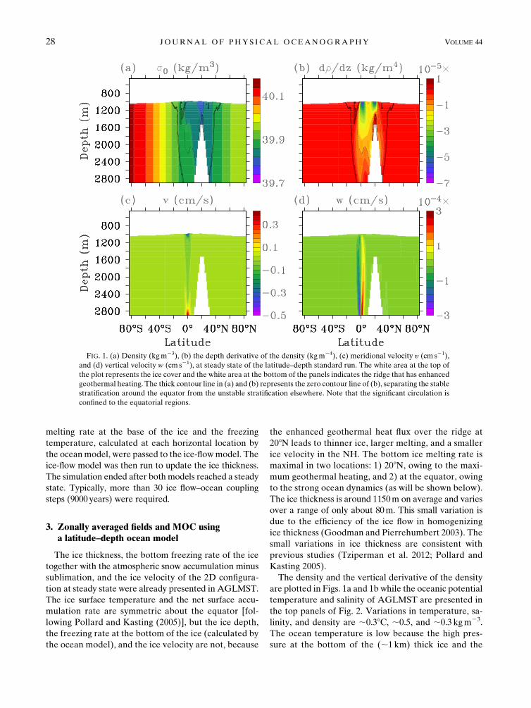
The density and the vertical derivative of the density

are plotted in Figs. 1a and 1b while the oceanic potential

temperature and salinity of AGLMST are presented in

the top panels of Fig. 2. Variations in temperature, sa-

linity, and density are ;0.38C, ;0.5, and ;0.3 kgm23.

The ocean temperature is low because the high pres-

sure at the bottom of the (;1 km) thick ice and the

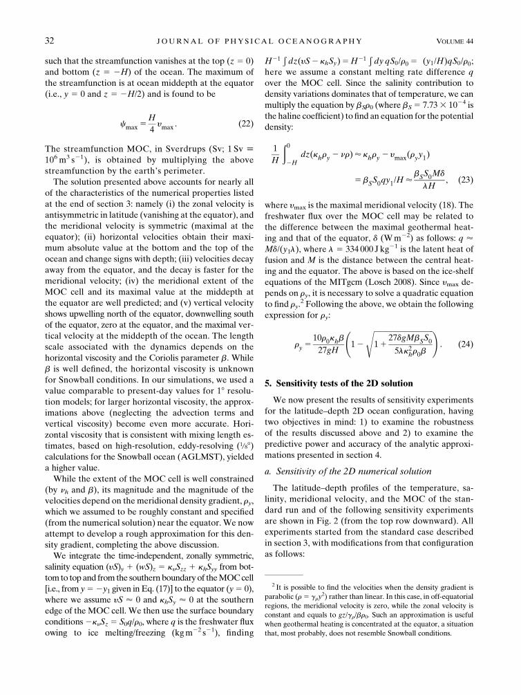
FIG. 1. (a) Density (kgm23), (b) the depth derivative of the density (kgm24), (c) meridional velocity y (cm s21),

and (d) vertical velocity w (cm s21), at steady state of the latitude–depth standard run. The white area at the top of

the plot represents the ice cover and the white area at the bottom of the panels indicates the ridge that has enhanced

geothermal heating. The thick contour line in (a) and (b) represents the zero contour line of (b), separating the stable

stratification around the equator from the unstable stratification elsewhere. Note that the significant circulation is

confined to the equatorial regions.


high salinity (;49.5) reduce the freezing temperature.

The small variations in temperature at the top of the

ocean (bottom of the ice), the large variations in sur-

face salinity, the similarity between the density and sa-

linity fields, and an analysis based on a linearized equation

of state all indicate that changes in density are dominated

by salinity variations. The changes in salinity are brought

about by melting over the enhanced geothermal heat

flux in the NH: the warmest water is close to the warm

ridge, and the freshest water is located above the top

of the ridge.

A notable feature of the solution is the vertically well-

mixed water column, except in the vicinity of the geo-

thermally heated ridge and the equator, where a very

weak stratification exists. This weak stratification is as-

sociated with meltwater at the base of the ice as a result

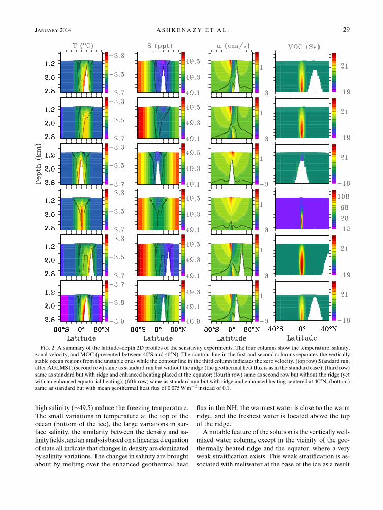
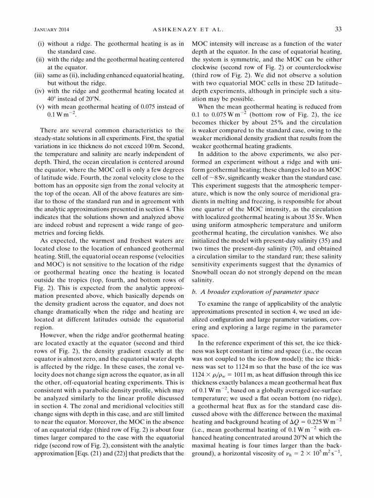
FIG. 2. A summary of the latitude–depth 2D profiles of the sensitivity experiments. The four columns show the temperature, salinity,

zonal velocity, and MOC (presented between 408S and 408N). The contour line in the first and second columns separates the vertically

stable ocean regions from the unstable ones while the contour line in the third column indicates the zero velocity. (top row) Standard run,

after AGLMST; (second row) same as standard run but without the ridge (the geothermal heat flux is as in the standard case); (third row)

same as standard but with ridge and enhanced heating placed at the equator; (fourth row) same as second row but without the ridge (yet

with an enhanced equatorial heating); (fifth row) same as standard run but with ridge and enhanced heating centered at 408N; (bottom)

same as standard but with mean geothermal heat flux of 0.075Wm22 instead of 0.1.


of the enhanced heating there. This is also related to the

zonal jets that are discussed below and in the next sec-

tion. The nearly vertically homogeneous potential den-

sity is used to simplify the analytic analysis in the next

section.

The zonal, meridional, and vertical velocities and the

MOC, are shown in Figs. 1c and 1d and in the top panel

of Fig. 2. Surprisingly, the counterclockwise circulation

is concentrated around the equator, while velocities away

from the equator, including over the ridge and enhanced

heating are very weak. This result is explained in the

next section. The simulated currents are not small, as

one would naively expect from a ‘‘stagnant’’ ocean under

Snowball Earth conditions (Kirschvink 1992), and the

intensity of the circulation is close to that of the pres-

ent day.

Several additional features of the solution are worth

noting: 1) there are two relatively strong and opposite

(antisymmetric) jets (of a few centimeters per second)

in the zonal velocity u (top row, third column of Fig. 2).

At the surface, we observe a westward current north of

the equator and an eastward current south of the equator.

Themeridional velocity (Fig. 1c) is symmetric around the

equator, with negative (southward) direction at the top of

the ocean and positive (northward) direction at the bot-

tom of the ocean. 2) The zonal and meridional velocities

are maximal (minimal) at the top (bottom) of the ocean,

change sign with depth, and vanish at the middle of the

ocean. 3) Both zonal and meridional velocities decay

away from the equator where the zonal velocity decays

much slower than the meridional and vertical velocities.

4) TheMOC (top panel of Fig. 2) streamfunction, implied

by the vertical and meridional velocities, is largest at the

equator and concentrated close to the equator. 5) The

vertical velocity w (Fig. 1d) is upward (positive) north of

the equator, downward (negative) south of the equator,

vanishes at the equator, and is maximal at ocean mid-

depth.

4. The dynamics of the equatorial MOCand zonal jets

Our goal in this section is to explain the dynamical

features listed in the previous section. We consider

the steady-state, zonally symmetric (x independent) hy-

drostatic equations. For simplicity, we use a Cartesian

coordinate system centered at the equator with an

equatorial b-plane approximation. Then, following the

numerical simulations, the advection and vertical vis-

cosity terms can be neglected from the momentum

equations (not shown). Apart from the fact that they

are found to be small in the numerical simulation, the

momentum advection terms and the vertical viscosity

may be shown to be small based on scaling arguments

(see the appendix). Based on the numerical results pre-

sented in section 3 and Fig. 1a, the density is assumed to

be independent of depth and the meridional density

(pressure) gradient is assumed to be approximately con-

stant near the equator.

The dominant momentum balances are found to be

2byy5 nhuyy , (3)

byu52py/r01 nhyyy, and (4)

pz52gr , (5)

where y and z are the meridional and depth coordinates,

u and y are the zonal and meridional velocities, b 5df/dy (where f is the Coriolis parameter), ny and nh are

the vertical and horizontal eddy-parameterized vis-

cosity coefficients, r is the density, r0 is the mean ocean

density, and g is the gravity constant. Vertically inte-

grating the hydrostatic equation and differentiating with

respect to y, we find that py52ryg[z1 F(y)], where z5 0

is defined to be at the ocean–ice interface and F(y) is

an arbitrary function of y so that

byu51

r0g[z1F(y)]ry1 nhyyy . (6)

It is possible to show that F(y) 5 H/2, by depth-

integrating Eqs. (3) and (6), using the fact that the

integrated meridional velocity should be zero due to

the mass (or volume) conservation and by assuming

that the depth-integrated zonal velocity vanishes at

y / 6‘.1

Equations (3) and (4) may be solved in terms of Airy

functions, but instead we solve them separately for the

off-equatorial and equatorial regions and then match

the two solutions, leading to a more informative solu-

tion. As shown in AGLMST, for the off-equatorial re-

gion, the viscosity term in Eq. (4) is negligible compared

to the Coriolis term, leading to

uoe5g(z1H/2)ry

br0

1

y. (7)

This leads, based on Eq. (3), to the following meridional

velocity away from the equator,

1 The integration of Eqs. (3) and (6) leads to2byV5 nhUyy 5 0

and hence U 5 rygH[F(y) 2 H/2]/(r0by) where U and V are the

vertically integrated velocities. Thus V 5 0 and U must be a linear

function of y. Since U must vanish when y / 6‘, F(y) 5 H/2 and

hence U 5 0 for every y.


yoe 522g(z1H/2)nhry

b2r0

1

y4, (8)

where the subscript oe stands for ‘‘off equatorial.’’

Based on Eqs. (7) and (8), it is clear that (i) both zonal

(i.e., u) and meridional (i.e., y) velocities decay away

from the equator, where y decays much faster than u;

(ii) u is antisymmetric about the equator, while y is

symmetric; and (iii) both u and y change signs at the

ocean middepth, z 5 2H/2.

In the equatorial region, the Coriolis term is negli-

gible in the meridional momentum balance, while it

still balances eddy viscosity in the zonal momentum

equation, so that Eqs. (3) and (4) become

nhue,yy 1byye 5 0 and (9)

1

r0g(z1H/2)ry 1 nhye,yy 5 0, (10)

where the subscript e denotes the equatorial solution.

These balances were verified from the numerical solu-

tion, and it was found that the eddy viscosity term

indeed varies linearly in latitude around the equator.

Continuing to assume, for simplicity, that the density

gradient term is approximately constant in latitude

near the equator, the solution is a second-order poly-

nomial for y and a fifth-order polynomial for u. Re-

quiring that the equatorial and off-equatorial solutions

match continuously at some latitude y0, one finds

ue 5gbry(z1H/2)

40r0n2h

y50

"y5

y501

40n2h3b2y60

210

3

!y3

y30

1

80n2h3b2y60

17

3

!y

y0

#and (11)

ye52gry(z1H/2)

2r0nhy20

y2

y201

4n2hb2

1

y602 1

!. (12)

It is clear that ue is antisymmetric in latitude, while ye is

symmetric, as in the off-equatorial region. The match-

ing point between the off-equatorial and the equatorial

velocities y0 can be found by requiring that the de-

rivative of the zonal velocity is continuous at y0 as well,

giving

y05 401/6�nhb

�. (13)

Using y0, the overall solution is

u(y)5

gbry(z1H/2)

40r0n2h

y50

y5

y502 3

y3

y301 3

y

y0

!, jyj, y0

g(z1H/2)ry

br0

1

y, jyj$ y0 ;

8>>>>><>>>>>:

and (14)

y(y)5

gry(z1H/2)

2r0nhy20

9

102

y2

y20

!, jyj, y0

22g(z1H/2)nhry

b2r0

1

y4, jyj$ y0 .

8>>>>><>>>>>:

(15)

The vertical velocity can be found from the continuity

equation

w(y)5

gry

2r0nh

�(z1H/2)22

H2

4

�y , jyj, y0 and

24gnhry

b2r0

�(z1H/2)22

H2

4

�1

y5, jyj$ y0 .

8>>>>><>>>>>:

(16)

Note that w is not continuous at y0.

The half-width of theMOC cell y1 can be estimated by

finding the location at which the meridional velocity

vanishes and is

y153ffiffiffiffiffi10

p y0 . (17)

The maximum meridional velocity ymax is found at the

equator, either at the top or the bottom of the ocean, as

ymax59gryH

40r0nhy20 . (18)

The mean meridional velocity within the MOC cell

boundaries is

hyi5 2

3ymax , (19)

where the angle brackets refer to the mean value. The

maximal zonal velocity umax can be shown to be either at

the surface or bottom of the ocean with a value of

umax’ 0:44ymax , (20)

at y*56y0

ffiffiffiffiffiffiffiffiffiffiffiffiffiffiffiffiffiffiffiffiffiffiffiffiffiffiffi(92

ffiffiffiffiffi21

p)/10

q’60:66y0.

The MOC streamfunction c(y, z) can be found by

integrating y(y, z) 5 2cz as

c(y, z)5gry

4r0nhy20

y2

y202

9

10

!�(z1H/2)22

H2

4

�(21)


such that the streamfunction vanishes at the top (z5 0)

and bottom (z 5 2H) of the ocean. The maximum of

the streamfunction is at ocean middepth at the equator

(i.e., y 5 0 and z 5 2H/2) and is found to be

cmax5H

4ymax . (22)

The streamfunction MOC, in Sverdrups (Sv; 1 Sv [106 m3 s21), is obtained by multiplying the above

streamfunction by the earth’s perimeter.

The solution presented above accounts for nearly all

of the characteristics of the numerical properties listed

at the end of section 3: namely (i) the zonal velocity is

antisymmetric in latitude (vanishing at the equator), and

the meridional velocity is symmetric (maximal at the

equator); (ii) horizontal velocities obtain their maxi-

mum absolute value at the bottom and the top of the

ocean and change signs with depth; (iii) velocities decay

away from the equator, and the decay is faster for the

meridional velocity; (iv) the meridional extent of the

MOC cell and its maximal value at the middepth at

the equator are well predicted; and (v) vertical velocity

shows upwelling north of the equator, downwelling south

of the equator, zero at the equator, and the maximal ver-

tical velocity at the middepth of the ocean. The length

scale associated with the dynamics depends on the

horizontal viscosity and the Coriolis parameter b. While

b is well defined, the horizontal viscosity is unknown

for Snowball conditions. In our simulations, we used a

value comparable to present-day values for 18 resolu-tion models; for larger horizontal viscosity, the approx-

imations above (neglecting the advection terms and

vertical viscosity) become even more accurate. Hori-

zontal viscosity that is consistent with mixing length es-

timates, based on high-resolution, eddy-resolving (1/88)calculations for the Snowball ocean (AGLMST), yielded

a higher value.

While the extent of the MOC cell is well constrained

(by nh and b), its magnitude and the magnitude of the

velocities depend on the meridional density gradient, ry,

which we assumed to be roughly constant and specified

(from the numerical solution) near the equator. We now

attempt to develop a rough approximation for this den-

sity gradient, completing the above discussion.

We integrate the time-independent, zonally symmetric,

salinity equation (yS)y 1 (wS)z 5 kySzz 1 khSyy from bot-

tom to top and from the southernboundaryof theMOCcell

[i.e., from y52y1 given in Eq. (17)] to the equator (y5 0),

where we assume yS ’ 0 and khSy ’ 0 at the southern

edge of the MOC cell. We then use the surface boundary

conditions2kySz5 S0q/r0, where q is the freshwater flux

owing to ice melting/freezing (kgm22 s21), finding

H21Ðdz(yS2 khSy)5H21

Ðdy qS0/r0 5 (y1/H)qS0/r0;

here we assume a constant melting rate difference q

over the MOC cell. Since the salinity contribution to

density variations dominates that of temperature, we can

multiply the equation by bSr0 (where bS5 7.733 1024 is

the haline coefficient) to find an equation for the potential

density:

1

H

ð02H

dz(khry2 nr)’ khry 2 ymax(ryy1)

5bSS0qy1/H’bSS0Md

lH, (23)

where ymax is the maximal meridional velocity (18). The

freshwater flux over the MOC cell may be related to

the difference between the maximal geothermal heat-

ing and that of the equator, d (Wm22) as follows: q ’Md/(y1l), where l 5 334 000 J kg21 is the latent heat of

fusion and M is the distance between the central heat-

ing and the equator. The above is based on the ice-shelf

equations of the MITgcm (Losch 2008). Since ymax de-

pends on ry, it is necessary to solve a quadratic equation

to find ry.2 Following the above, we obtain the following

expression for ry:

ry510r0khb

27gH

12

ffiffiffiffiffiffiffiffiffiffiffiffiffiffiffiffiffiffiffiffiffiffiffiffiffiffiffiffiffiffiffiffiffi11

27dgMbSS05lk2hr0b

s !. (24)

5. Sensitivity tests of the 2D solution

We now present the results of sensitivity experiments

for the latitude–depth 2D ocean configuration, having

two objectives in mind: 1) to examine the robustness

of the results discussed above and 2) to examine the

predictive power and accuracy of the analytic approxi-

mations presented in section 4.

a. Sensitivity of the 2D numerical solution

The latitude–depth profiles of the temperature, sa-

linity, meridional velocity, and the MOC of the stan-

dard run and of the following sensitivity experiments

are shown in Fig. 2 (from the top row downward). All

experiments started from the standard case described

in section 3, with modifications from that configuration

as follows:

2 It is possible to find the velocities when the density gradient is

parabolic (r 5 gry2) rather than linear. In this case, in off-equatorial

regions, the meridional velocity is zero, while the zonal velocity is

constant and equals to gz/gr/br0. Such an approximation is useful

when geothermal heating is concentrated at the equator, a situation

that, most probably, does not resemble Snowball conditions.


(i) without a ridge. The geothermal heating is as in

the standard case.

(ii) with the ridge and the geothermal heating centered

at the equator.

(iii) same as (ii), including enhanced equatorial heating,

but without the ridge.

(iv) with the ridge and geothermal heating located at

408 instead of 208N.

(v) with mean geothermal heating of 0.075 instead of

0.1Wm22.

There are several common characteristics to the

steady-state solutions in all experiments. First, the spatial

variations in ice thickness do not exceed 100m. Second,

the temperature and salinity are nearly independent of

depth. Third, the ocean circulation is centered around

the equator, where the MOC cell is only a few degrees

of latitude wide. Fourth, the zonal velocity close to the

bottom has an opposite sign from the zonal velocity at

the top of the ocean. All of the above features are sim-

ilar to those of the standard run and in agreement with

the analytic approximations presented in section 4. This

indicates that the solutions shown and analyzed above

are indeed robust and represent a wide range of geo-

metries and forcing fields.

As expected, the warmest and freshest waters are

located close to the location of enhanced geothermal

heating. Still, the equatorial ocean response (velocities

and MOC) is not sensitive to the location of the ridge

or geothermal heating once the heating is located

outside the tropics (top, fourth, and bottom rows of

Fig. 2). This is expected from the analytic approxi-

mation presented above, which basically depends on

the density gradient across the equator, and does not

change dramatically when the ridge and heating are

located at different latitudes outside the equatorial

region.

However, when the ridge and/or geothermal heating

are located exactly at the equator (second and third

rows of Fig. 2), the density gradient exactly at the

equator is almost zero, and the equatorial water depth

is affected by the ridge. In these cases, the zonal ve-

locity does not change sign across the equator, as in all

the other, off-equatorial heating experiments. This is

consistent with a parabolic density profile, which may

be analyzed similarly to the linear profile discussed

in section 4. The zonal and meridional velocities still

change signs with depth in this case, and are still limited

to near the equator. Moreover, the MOC in the absence

of an equatorial ridge (third row of Fig. 2) is about four

times larger compared to the case with the equatorial

ridge (second row of Fig. 2), consistent with the analytic

approximation [Eqs. (21) and (22)] that predicts that the

MOC intensity will increase as a function of the water

depth at the equator. In the case of equatorial heating,

the system is symmetric, and the MOC can be either

clockwise (second row of Fig. 2) or counterclockwise

(third row of Fig. 2). We did not observe a solution

with two equatorial MOC cells in these 2D latitude–

depth experiments, although in principle such a situ-

ation may be possible.

When the mean geothermal heating is reduced from

0.1 to 0.075Wm22 (bottom row of Fig. 2), the ice

becomes thicker by about 25% and the circulation

is weaker compared to the standard case, owing to the

weaker meridional density gradient that results from the

weaker geothermal heating gradients.

In addition to the above experiments, we also per-

formed an experiment without a ridge and with uni-

form geothermal heating; these changes led to anMOC

cell of;8 Sv, significantly weaker than the standard case.

This experiment suggests that the atmospheric temper-

ature, which is now the only source of meridional gra-

dients in melting and freezing, is responsible for about

one quarter of the MOC intensity, as the circulation

with localized geothermal heating is about 35 Sv. When

using uniform atmospheric temperature and uniform

geothermal heating, the circulation vanishes. We also

initialized the model with present-day salinity (35) and

two times the present-day salinity (70), and obtained

a circulation similar to the standard run; these salinity

sensitivity experiments suggest that the dynamics of

Snowball ocean do not strongly depend on the mean

salinity.

b. A broader exploration of parameter space

To examine the range of applicability of the analytic

approximations presented in section 4, we used an ide-

alized configuration and large parameter variations, cov-

ering and exploring a large regime in the parameter

space.

In the reference experiment of this set, the ice thick-

ness was kept constant in time and space (i.e., the ocean

was not coupled to the ice-flow model); the ice thick-

ness was set to 1124m so that the base of the ice was

1124 3 ri/rw 5 1011m, as heat diffusion through this ice

thickness exactly balances a mean geothermal heat flux

of 0.1Wm22, based on a globally averaged ice-surface

temperature; we used a flat ocean bottom (no ridge),

a geothermal heat flux as for the standard case dis-

cussed above with the difference between the maximal

heating and background heating of DQ 5 0.225Wm22

(i.e., mean geothermal heating of 0.1Wm22 with en-

hanced heating concentrated around 208N at which the

maximal heating is four times larger than the back-

ground), a horizontal viscosity of nh 5 2 3 105m2 s21,


a vertical viscosity of ny 5 2 3 1023m2 s21, horizontal

and vertical diffusion coefficients of temperature and

salinity of kh 5 2000m2 s21 and ky 5 2 3 1024 m2 s21,

and an ocean depth ofH5 2000m.We used a latitude–

depth configuration with a meridional extent from 848Sto 848N and 28 resolution (the edge grid points are as-

sumed to be land points); 21 vertical levels were used,

with an upper level, completely embedded within the

ice, having thickness of 1 km and additional 20 levels,

each of them 100m thick. The different experiments

were run until a steady state was reached.

We performed the following experiments, all starting

from the reference experiment described above with

the following modifications:

1) Reference experiment as described above.

2) A 10 times deeper ocean, 10H.

3) A 10 times shallower ocean, H/10.

4) Uniform geothermal heat flux, DQ 5 0.

5) Difference between the maximal geothermal heat

flux and the background of 3DQ’ 0.608Wm22; the

maximum heat flux is 18 times larger than the

background.

6) Rotation that is 1/4 of the earth’s rotation (i.e., the

b-plane coefficient becomes b/4).

7) Rotation that is 1/9 of the earth’s rotation (i.e., the

b-plane coefficient becomes b/9).

8) A 16 times larger horizontal viscosity coefficient, 16nh.

9) A 4 times smaller horizontal viscosity coefficient, nh/4.

10) A 4 times larger horizontal diffusion coefficient, 4kh.

11) A 4 times smaller horizontal diffusion coefficient, kh/4.

12) A 16 times larger horizontal viscosity coefficient,

16nh, and 4 times larger horizontal diffusion co-

efficient, 4kh.

13) A 4 times larger horizontal viscosity coefficient, 4nh,

and 4 times larger horizontal diffusion coefficient,

4kh.

14) A 10 times smaller vertical diffusion coefficient, ky/10.

15) A 4 times smaller horizontal viscosity coefficient,

nh/4, and a 4 times smaller horizontal diffusion

coefficient, kh/4.

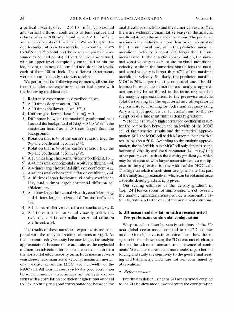
The results of these numerical experiments are com-

pared with the analytical scaling solutions in Fig. 3. As

the horizontal eddy viscosity becomes larger, the analytic

approximations become more accurate, as the neglected

momentum advection terms become even smaller than

the horizontal eddy viscosity term. Four measures were

considered: maximum zonal velocity, maximum meridi-

onal velocity, maximum MOC, and half-width of the

MOC cell. All four measures yielded a good correlation

between numerical experiments and analytic expres-

sions with a correlation coefficient higher than or equal

to 0.87, pointing to a good correspondence between the

analytic approximations and the numerical results. Yet,

there are systematic quantitative biases in the analytic

results relative to the numerical solutions. The predicted

maximal zonal velocity is more than two times smaller

than the numerical one, while the predicted maximal

meridional velocity is about 30% larger than the nu-

merical one. In the analytic approximation, the maxi-

mal zonal velocity is 44% of the maximal meridional

velocity, while in the numerical simulations the maxi-

mal zonal velocity is larger than 67% of the maximal

meridional velocity. Similarly, the predicted maximal

MOC is 30% larger than the numerical one. The dif-

ference between the numerical and analytic approxi-

mations may be attributed to the terms neglected in

the analytic approximation, to the piecewise analytic

solution (solving for the equatorial and off-equatorial

regions instead of solving for both simultaneously using

Airy and hypergeometrical functions), and to the as-

sumption of a linear latitudinal density gradient.

We found a relatively high correlation coefficient of 0.95

for the comparison between the half-width of the MOC

cell of the numerical results and the numerical approxi-

mation. Still, theMOC cell width is larger in the numerical

results by about 50%. According to the analytic approxi-

mation, the half-width in theMOCcell only depends on the

horizontal viscosity and the b parameter [i.e., }(nh/b)1/3];

other parameters, such as the density gradient ry, which

may be associated with larger uncertainties, do not ap-

pear in the expression for the width of the MOC cell.

This high correlation coefficient strengthens the first part

of the analytic approximation, which can be obtained once

a specific density gradient ry is given.

Our scaling estimate of the density gradient ry[Eq. (24)] leaves room for improvement. Yet, overall,

the analytic approximations provide a reasonable es-

timate, within a factor of 2, of the numerical solutions.

6. 3D ocean model solution with a reconstructedNeoproterozoic continental configuration

We proceed to describe steady solutions of the 3D

near-global ocean model coupled to the 2D ice-flow

model. Our objective is to examine if and how the in-

sights obtained above, using the 2D ocean model, change

due to the added dimension and presence of conti-

nents. We can also examine a more realistic geothermal

forcing and study the sensitivity to the geothermal heat-

ing and bathymetry, which are not well constrained by

observations.

a. Reference state

For the simulation using the 3D ocean model coupled

to the 2D ice-flow model, we followed the configuration


described in section 2. Our standard 3D run included

enhanced localized geothermal heating along spreading

centers following Li et al. (2008), as indicated by the

solid black contour line in Fig. 4.

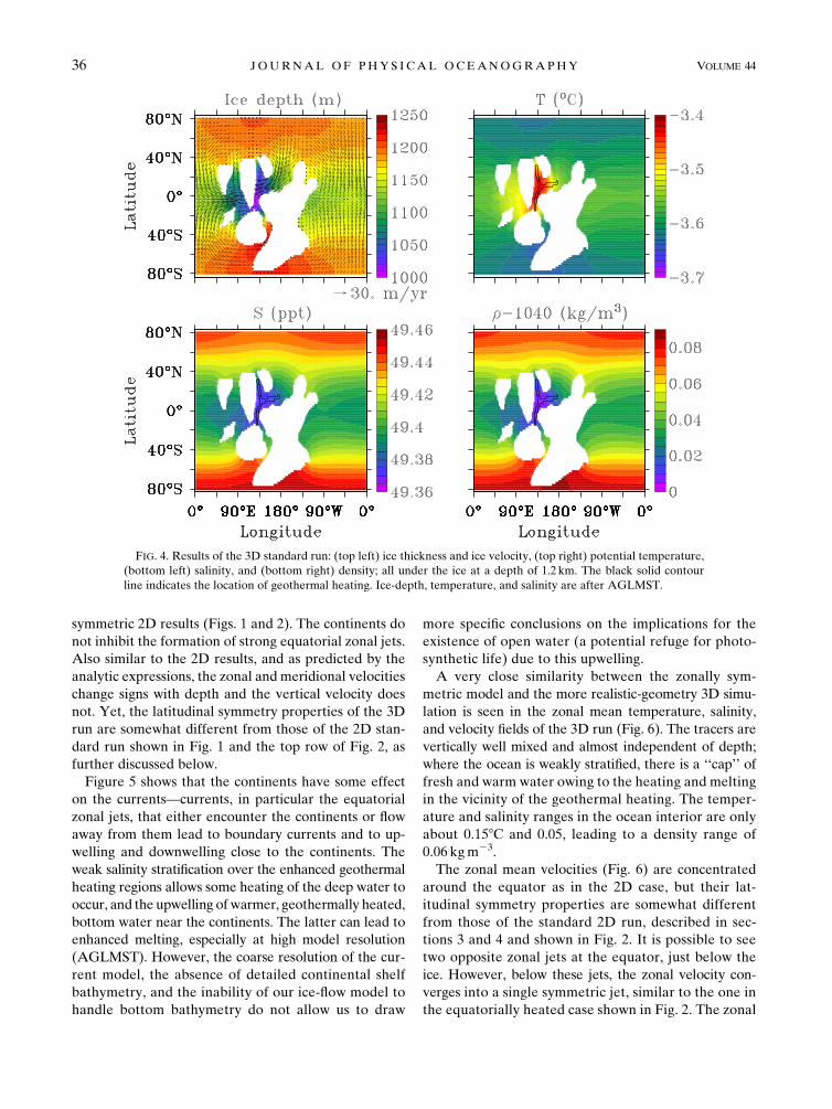
The ice thickness and velocity field are shown in Fig. 4a.

The ice is generally thicker than 1km. As in Tziperman

et al. (2012), the ice is thinner in the constricted sea area

between the landmasses, both owing to the ice sublimation

and melting there (see below) and due to the reduced ice

flow into this region because of the friction with the

landmasses. The differences in ice thickness can reach

240m, significantly more than in the 1D case without

continents (Campbell et al. 2011; Tziperman et al.

2012). As expected, the general ice flow is directed

from the high latitudes toward the equator (i.e., from

snow/ice accumulation areas to ice sublimation/melting

areas) with a velocity of up to 35myr21 in the region of

the constricted sea.

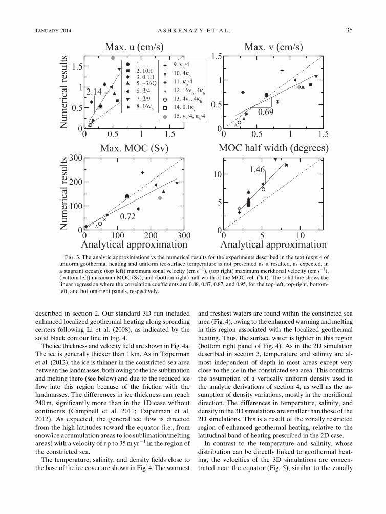
The temperature, salinity, and density fields close to

the base of the ice cover are shown in Fig. 4. The warmest

and freshest waters are found within the constricted sea

area (Fig. 4), owing to the enhancedwarming andmelting

in this region associated with the localized geothermal

heating. Thus, the surface water is lighter in this region

(bottom right panel of Fig. 4). As in the 2D simulation

described in section 3, temperature and salinity are al-

most independent of depth in most areas except very

close to the ice in the constricted sea area. This confirms

the assumption of a vertically uniform density used in

the analytic derivations of section 4, as well as the as-

sumption of density variations, mostly in the meridional

direction. The differences in temperature, salinity, and

density in the 3D simulations are smaller than those of the

2D simulations. This is a result of the zonally restricted

region of enhanced geothermal heating, relative to the

latitudinal band of heating prescribed in the 2D case.

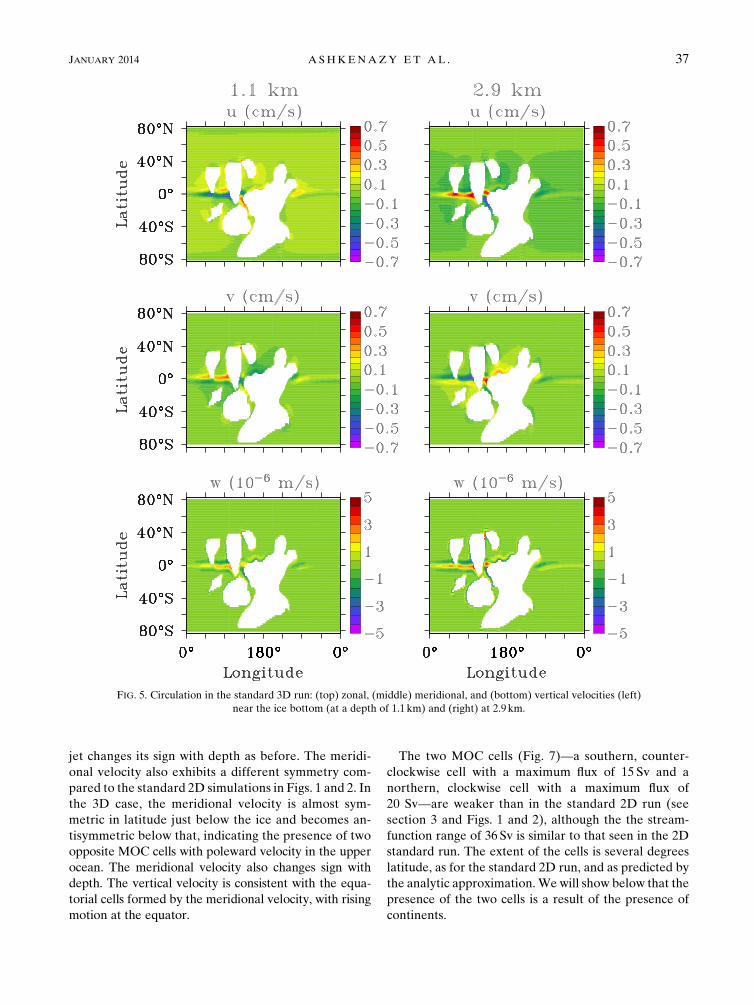
In contrast to the temperature and salinity, whose

distribution can be directly linked to geothermal heat-

ing, the velocities of the 3D simulations are concen-

trated near the equator (Fig. 5), similar to the zonally

FIG. 3. The analytic approximations vs the numerical results for the experiments described in the text (expt 4 of

uniform geothermal heating and uniform ice-surface temperature is not presented as it resulted, as expected, in

a stagnant ocean): (top left) maximum zonal velocity (cm s21), (top right) maximum meridional velocity (cm s21),

(bottom left) maximum MOC (Sv), and (bottom right) half-width of the MOC cell (8lat). The solid line shows the

linear regression where the correlation coefficients are 0.88, 0.87, 0.87, and 0.95, for the top-left, top-right, bottom-

left, and bottom-right panels, respectively.


symmetric 2D results (Figs. 1 and 2). The continents do

not inhibit the formation of strong equatorial zonal jets.

Also similar to the 2D results, and as predicted by the

analytic expressions, the zonal and meridional velocities

change signs with depth and the vertical velocity does

not. Yet, the latitudinal symmetry properties of the 3D

run are somewhat different from those of the 2D stan-

dard run shown in Fig. 1 and the top row of Fig. 2, as

further discussed below.

Figure 5 shows that the continents have some effect

on the currents—currents, in particular the equatorial

zonal jets, that either encounter the continents or flow

away from them lead to boundary currents and to up-

welling and downwelling close to the continents. The

weak salinity stratification over the enhanced geothermal

heating regions allows some heating of the deep water to

occur, and the upwelling of warmer, geothermally heated,

bottom water near the continents. The latter can lead to

enhanced melting, especially at high model resolution

(AGLMST). However, the coarse resolution of the cur-

rent model, the absence of detailed continental shelf

bathymetry, and the inability of our ice-flow model to

handle bottom bathymetry do not allow us to draw

more specific conclusions on the implications for the

existence of open water (a potential refuge for photo-

synthetic life) due to this upwelling.

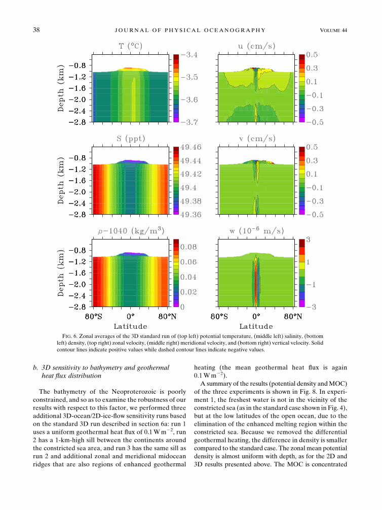
A very close similarity between the zonally sym-

metric model and the more realistic-geometry 3D simu-

lation is seen in the zonal mean temperature, salinity,

and velocity fields of the 3D run (Fig. 6). The tracers are

vertically well mixed and almost independent of depth;

where the ocean is weakly stratified, there is a ‘‘cap’’ of

fresh and warm water owing to the heating and melting

in the vicinity of the geothermal heating. The temper-

ature and salinity ranges in the ocean interior are only

about 0.158C and 0.05, leading to a density range of

0.06 kgm23.

The zonal mean velocities (Fig. 6) are concentrated

around the equator as in the 2D case, but their lat-

itudinal symmetry properties are somewhat different

from those of the standard 2D run, described in sec-

tions 3 and 4 and shown in Fig. 2. It is possible to see

two opposite zonal jets at the equator, just below the

ice. However, below these jets, the zonal velocity con-

verges into a single symmetric jet, similar to the one in

the equatorially heated case shown in Fig. 2. The zonal

FIG. 4. Results of the 3D standard run: (top left) ice thickness and ice velocity, (top right) potential temperature,

(bottom left) salinity, and (bottom right) density; all under the ice at a depth of 1.2 km. The black solid contour

line indicates the location of geothermal heating. Ice-depth, temperature, and salinity are after AGLMST.


jet changes its sign with depth as before. The meridi-

onal velocity also exhibits a different symmetry com-

pared to the standard 2D simulations in Figs. 1 and 2. In

the 3D case, the meridional velocity is almost sym-

metric in latitude just below the ice and becomes an-

tisymmetric below that, indicating the presence of two

opposite MOC cells with poleward velocity in the upper

ocean. The meridional velocity also changes sign with

depth. The vertical velocity is consistent with the equa-

torial cells formed by the meridional velocity, with rising

motion at the equator.

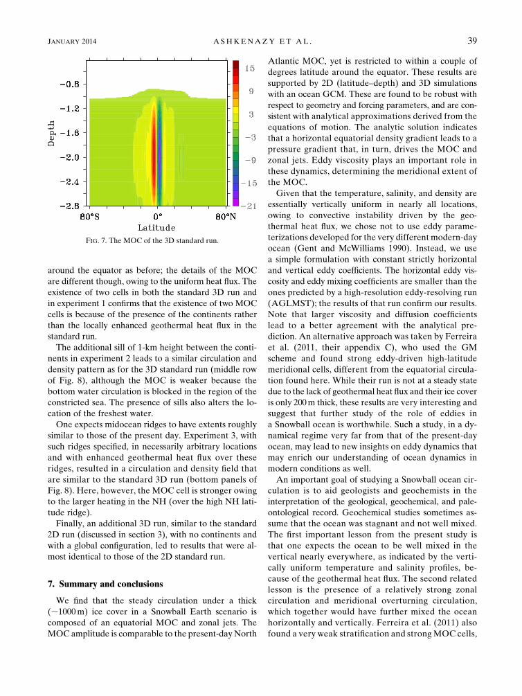
The two MOC cells (Fig. 7)—a southern, counter-

clockwise cell with a maximum flux of 15 Sv and a

northern, clockwise cell with a maximum flux of

20 Sv—are weaker than in the standard 2D run (see

section 3 and Figs. 1 and 2), although the the stream-

function range of 36 Sv is similar to that seen in the 2D

standard run. The extent of the cells is several degrees

latitude, as for the standard 2D run, and as predicted by

the analytic approximation.We will show below that the

presence of the two cells is a result of the presence of

continents.

FIG. 5. Circulation in the standard 3D run: (top) zonal, (middle) meridional, and (bottom) vertical velocities (left)

near the ice bottom (at a depth of 1.1 km) and (right) at 2.9 km.


b. 3D sensitivity to bathymetry and geothermalheat flux distribution

The bathymetry of the Neoproterozoic is poorly

constrained, and so as to examine the robustness of our

results with respect to this factor, we performed three

additional 3D-ocean/2D-ice-flow sensitivity runs based

on the standard 3D run described in section 6a: run 1

uses a uniform geothermal heat flux of 0.1Wm22, run

2 has a 1-km-high sill between the continents around

the constricted sea area, and run 3 has the same sill as

run 2 and additional zonal and meridional midocean

ridges that are also regions of enhanced geothermal

heating (the mean geothermal heat flux is again

0.1Wm22).

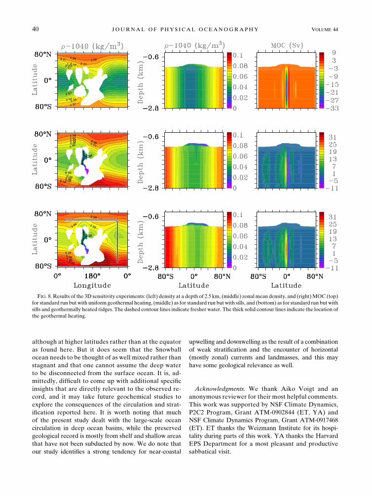
A summary of the results (potential density andMOC)

of the three experiments is shown in Fig. 8. In experi-

ment 1, the freshest water is not in the vicinity of the

constricted sea (as in the standard case shown in Fig. 4),

but at the low latitudes of the open ocean, due to the

elimination of the enhanced melting region within the

constricted sea. Because we removed the differential

geothermal heating, the difference in density is smaller

compared to the standard case. The zonal mean potential

density is almost uniform with depth, as for the 2D and

3D results presented above. The MOC is concentrated

FIG. 6. Zonal averages of the 3D standard run of (top left) potential temperature, (middle left) salinity, (bottom

left) density, (top right) zonal velocity, (middle right) meridional velocity, and (bottom right) vertical velocity. Solid

contour lines indicate positive values while dashed contour lines indicate negative values.


around the equator as before; the details of the MOC

are different though, owing to the uniform heat flux. The

existence of two cells in both the standard 3D run and

in experiment 1 confirms that the existence of two MOC

cells is because of the presence of the continents rather

than the locally enhanced geothermal heat flux in the

standard run.

The additional sill of 1-km height between the conti-

nents in experiment 2 leads to a similar circulation and

density pattern as for the 3D standard run (middle row

of Fig. 8), although the MOC is weaker because the

bottom water circulation is blocked in the region of the

constricted sea. The presence of sills also alters the lo-

cation of the freshest water.

One expects midocean ridges to have extents roughly

similar to those of the present day. Experiment 3, with

such ridges specified, in necessarily arbitrary locations

and with enhanced geothermal heat flux over these

ridges, resulted in a circulation and density field that

are similar to the standard 3D run (bottom panels of

Fig. 8). Here, however, the MOC cell is stronger owing

to the larger heating in the NH (over the high NH lati-

tude ridge).

Finally, an additional 3D run, similar to the standard

2D run (discussed in section 3), with no continents and

with a global configuration, led to results that were al-

most identical to those of the 2D standard run.

7. Summary and conclusions

We find that the steady circulation under a thick

(;1000m) ice cover in a Snowball Earth scenario is

composed of an equatorial MOC and zonal jets. The

MOC amplitude is comparable to the present-day North

Atlantic MOC, yet is restricted to within a couple of

degrees latitude around the equator. These results are

supported by 2D (latitude–depth) and 3D simulations

with an ocean GCM. These are found to be robust with

respect to geometry and forcing parameters, and are con-

sistent with analytical approximations derived from the

equations of motion. The analytic solution indicates

that a horizontal equatorial density gradient leads to a

pressure gradient that, in turn, drives the MOC and

zonal jets. Eddy viscosity plays an important role in

these dynamics, determining the meridional extent of

the MOC.

Given that the temperature, salinity, and density are

essentially vertically uniform in nearly all locations,

owing to convective instability driven by the geo-

thermal heat flux, we chose not to use eddy parame-

terizations developed for the very different modern-day

ocean (Gent and McWilliams 1990). Instead, we use

a simple formulation with constant strictly horizontal

and vertical eddy coefficients. The horizontal eddy vis-

cosity and eddy mixing coefficients are smaller than the

ones predicted by a high-resolution eddy-resolving run

(AGLMST); the results of that run confirm our results.

Note that larger viscosity and diffusion coefficients

lead to a better agreement with the analytical pre-

diction. An alternative approach was taken by Ferreira

et al. (2011, their appendix C), who used the GM

scheme and found strong eddy-driven high-latitude

meridional cells, different from the equatorial circula-

tion found here. While their run is not at a steady state

due to the lack of geothermal heat flux and their ice cover

is only 200m thick, these results are very interesting and

suggest that further study of the role of eddies in

a Snowball ocean is worthwhile. Such a study, in a dy-

namical regime very far from that of the present-day

ocean, may lead to new insights on eddy dynamics that

may enrich our understanding of ocean dynamics in

modern conditions as well.

An important goal of studying a Snowball ocean cir-

culation is to aid geologists and geochemists in the

interpretation of the geological, geochemical, and pale-

ontological record. Geochemical studies sometimes as-

sume that the ocean was stagnant and not well mixed.

The first important lesson from the present study is

that one expects the ocean to be well mixed in the

vertical nearly everywhere, as indicated by the verti-

cally uniform temperature and salinity profiles, be-

cause of the geothermal heat flux. The second related

lesson is the presence of a relatively strong zonal

circulation and meridional overturning circulation,

which together would have further mixed the ocean

horizontally and vertically. Ferreira et al. (2011) also

found a very weak stratification and strongMOC cells,

FIG. 7. The MOC of the 3D standard run.


although at higher latitudes rather than at the equator

as found here. But it does seem that the Snowball

ocean needs to be thought of as well mixed rather than

stagnant and that one cannot assume the deep water

to be disconnected from the surface ocean. It is, ad-

mittedly, difficult to come up with additional specific

insights that are directly relevant to the observed re-

cord, and it may take future geochemical studies to

explore the consequences of the circulation and strat-

ification reported here. It is worth noting that much

of the present study dealt with the large-scale ocean

circulation in deep ocean basins, while the preserved

geological record is mostly from shelf and shallow areas

that have not been subducted by now. We do note that

our study identifies a strong tendency for near-coastal

upwelling and downwelling as the result of a combination

of weak stratification and the encounter of horizontal

(mostly zonal) currents and landmasses, and this may

have some geological relevance as well.

Acknowledgments. We thank Aiko Voigt and an

anonymous reviewer for their most helpful comments.

This work was supported by NSF Climate Dynamics,

P2C2 Program, Grant ATM-0902844 (ET, YA) and

NSF Climate Dynamics Program, Grant ATM-0917468

(ET). ET thanks the Weizmann Institute for its hospi-

tality during parts of this work. YA thanks the Harvard

EPS Department for a most pleasant and productive

sabbatical visit.

FIG. 8. Results of the 3D sensitivity experiments: (left) density at a depth of 2.5 km, (middle) zonal mean density, and (right)MOC (top)

for standard run but with uniform geothermal heating, (middle) as for standard run but with sills, and (bottom) as for standard run but with

sills and geothermally heated ridges. The dashed contour lines indicate fresher water. The thick solid contour lines indicate the location of

the geothermal heating.


APPENDIX

Scaling of Idealized 2D Configuration

We start from the b-plane momentum equations un-

der the assumptions of steady state (i.e., ›t5 0 and zonal

symmetry ›x 5 0):

yuy1wuz2byy5 nhuyy 1 nyuzz and (A1)

yyy 1wyz1byu521

r0py1 nhyyy1 nyyzz . (A2)

It is possible to switch to nondimensional variables as

follows: y5 (nh/b)1/3y, z5Hz (H is the depth of the

ocean), p5 gHry(nh/b)1/3p, u5 (gHry)/(r0b

2/3n1/3h )u,

y5 (gHry)/(r0b2/3n1/3h )y, and w5 (gH2ry)/(r0b1/3n2/3h )w,

where the caret indicates nondimensional variables.

Then Eqs. (A1) and (A2) become

«1yuy1 «1wuz2 yy5 uyy 1 «2uzz and (A3)

«1yyy1 «1wyz1 yu52py1 yyy1 «2yzz , (A4)

where

«15gHry

r0bnh� 1 and (A5)

«25ny

H2b2/3n1/3h

� 1 (A6)

are small parameters under our choice of parameters,

;8 3 1023 and ;2 3 1025, respectively. Thus, it is pos-

sible to neglect the advection and vertical viscosity terms

from the momentum equations.

REFERENCES

Abbot, D. S., and I. Halevy, 2010: Dust aerosol important for

Snowball Earth deglaciation. J. Climate, 23, 4121–4132.

——, and R. T. Pierrehumbert, 2010: Mudball: Surface dust and

Snowball Earth deglaciation. J. Geophys. Res., 115, D03104,

doi:10.1029/2009JD012007.

——, A. Voigt, and D. Koll, 2011: The Jormungand global climate

state and implications for Neoproterozoic glaciations. J. Geo-

phys. Res., 116, D18103, doi:10.1029/2011JD015927.

——, ——, M. Branson, R. T. Pierrehumbert, D. Pollard, G. Le

Hir, and D. D. Koll, 2012: Clouds and Snowball Earth

deglaciation. Geophys. Res. Lett., 39, L20711, doi:10.1029/

2012GL052861.

Allen, P. A., and J. L. Etienne, 2008: Sedimentary challenge to

Snowball Earth. Nat. Geosci., 1, 817–825.Ashkenazy, Y., H. Gildor, M. Losch, F. A.Macdonald, D. P. Schrag,

and E. Tziperman, 2013: Dynamics of a Snowball Earth ocean.

Nature, 495, 90–93, doi:10.1038/nature11894.

Baum, S., and T. Crowley, 2001: GCM response to late Precambrian

(similar to 590 ma) ice-covered continents. Geophys. Res. Lett.,

28, 583–586.

——, and ——, 2003: The snow/ice instability as a mechanism for

rapid climate change: A Neoproterozoic Snowball Earth

model example. Geophys. Res. Lett., 30, 2030, doi:10.1029/

2003GL017333.

Bryan, K., 1984: Accelerating the convergence to equilibrium of

ocean–climate models. J. Phys. Oceanogr., 14, 666–673.Budyko, M. I., 1969: The effect of solar radiation variations on

the climate of the earth. Tellus, 21, 611–619.

Campbell, A. J., E. D. Waddington, and S. G. Warren, 2011: Re-

fugium for surface life on Snowball Earth in a nearly-enclosed

sea? A first simple model for sea-glacier invasion. Geophys.

Res. Lett., 38, L19502, doi:10.1029/2011GL048846.

Chandler, M. A., and L. E. Sohl, 2000: Climate forcings and the initi-

ation of low-latitude ice sheets during the Neoproterozoic Var-

anger glacial interval. J. Geophys. Res., 105 (D16), 20737–20756.

Crowley, T., and S. Baum, 1993: Effect of decreased solar lumi-

nosity on late Precambrian ice extent. J.Geophys. Res., 98 (D9),

16 723–16 732.

Donnadieu, Y., F. Fluteau, G. Ramstein, C. Ritz, and J. Besse,

2003: Is there a conflict between the Neoproterozoic glacial

deposits and the Snowball Earth interpretation: An improved

understanding with numerical modeling. Earth Planet. Sci.

Lett., 208, 101–112.——, Y. Godderis, G. Ramstein, A. Nedelec, and J. Meert, 2004a:

A ‘Snowball Earth’ climate triggered by continental break-up

through changes in runoff. Nature, 428, 303–306.

——, G. Ramstein, F. Fluteau, D. Roche, and A. Ganopolski,

2004b: The impact of atmospheric and oceanic heat transports

on the sea-ice–albedo instability during the Neoproterozoic.

Climate Dyn., 22, 293–306.

Evans, D. A. D., and T. D. Raub, 2011: Neoproterozoic glacial

palaeolatitudes: A global update. The Geological Record of

Neoproterozoic Glaciations, E. Arnaud, G. P. Halverson, and

G. Shields-Zhou, Eds., Geological Society of London, 93–112.

Ferreira, D., J. Marshall, and B. E. J. Rose, 2011: Climate de-

terminism revisited: Multiple equilibria in a complex climate

model. J. Climate, 24, 992–1012.

Gent, P. R., and J. C. McWilliams, 1990: Isopycnal mixing in ocean

circulation models. J. Phys. Oceanogr., 20, 150–155.

Goodman, J. C., 2006: Through thick and thin: Marine and mete-

oric ice in a ‘‘Snowball Earth’’ climate.Geophys. Res. Lett., 33,

L16701, doi:10.1029/2006GL026840.

——, and R. T. Pierrehumbert, 2003: Glacial flow of floating ma-

rine ice in ‘‘Snowball Earth.’’ J. Geophys. Res., 108, 3308,

doi:10.1029/2002JC001471.

Harland, W. B., 1964: Evidence of late Precambrian glaciation and

its significance. Problems in Palaeoclimatology,A. E. M. Nairn,

Ed., John Wiley & Sons, 119–149 and 180–184.

Hoffman, P., and D. Schrag, 2002: The Snowball Earth hypothesis:

Testing the limits of global change. Terra Nova, 14, 129–155,

doi:10.1046/j.1365-3121.2002.00408.x.

Hyde, W. T., T. J. Crowley, S. K. Baum, and W. R. Peltier, 2000:

Neoproterozoic ‘Snowball Earth’ simulations with a coupled

climate/ice-sheet model. Nature, 405, 425–429.

Jackett, D. R., and T. J. McDougall, 1995: Minimal adjustment of

hydrographic profiles to achieve static stability. J. Atmos. Oce-

anic Technol., 12, 381–389.Jenkins, G., and S. Smith, 1999: GCM simulations of Snowball

Earth conditions during the late Proterozoic. Geophys. Res.

Lett., 26, 2263–2266.


Kirschvink, J. L., 1992: Late Proterozoic low-latitude glaciation:

The Snowball Earth. The Proterozoic Biosphere, J. W. Schopf

and C. Klein, Eds., Cambridge University Press, 51–52.

Knauth, L., 2005: Temperature and salinity history of the Pre-

cambrian ocean: Implications for the course of microbial evo-

lution. Palaeogeogr. Palaeoclimatol. Palaeoecol., 219, 53–69.Langen, P. L., and V. A. Alexeev, 2004: Multiple equilibria and

asymmetric climates in the CCM3 coupled to an oceanic mixed

layer with thermodynamic sea ice. Geophys. Res. Lett., 31,

L04201, doi:10.1029/2003GL019039.

Le Hir, G., G. Ramstein, Y. Donnadieu, and R. T. Pierrehumbert,

2007: Investigating plausible mechanisms to trigger a deglacia-

tion from a hard Snowball Earth. C. R. Geosci., 339, 274–287,

doi:10.1016/j.crte.2006.09.002.

——, Y. Donnadieu, G. Krinner, and G. Ramstein, 2010: Toward

the Snowball Earth deglaciation. . . Climate Dyn., 35, 285–297,

doi:10.1007/s00382-010-0748-8.

Lewis, J. P., A. J. Weaver, S. T. Johnston, and M. Eby, 2003:

Neoproterozoic ‘‘Snowball Earth’’: Dynamic sea ice over a

quiescent ocean. Paleoceanography, 18, 1092, doi:10.1029/

2003PA000926.

——, M. Eby, A. J. Weaver, S. Johnston, and R. Jacob, 2004:

Global glaciation in theNeoproterozoic: Reconciling previous

modelling results.Geophys. Res. Lett., 31, L08201, doi:10.1029/

2004GL019725.

——, A. J. Weaver, and M. Eby, 2007: Snowball versus slushball

Earth: Dynamic versus nondynamic sea ice? J. Geophys. Res.,

112, C11014, doi:10.1029/2006JC004037.

Li, D., and R. T. Pierrehumbert, 2011: Sea glacier flow and dust

transport on Snowball Earth.Geophys. Res. Lett., 38, L17501,

doi:10.1029/2011GL048991.

Li, Z. X., and Coauthors, 2008: Assembly, configuration, and

break-up history of Rodinia: A synthesis. Precambrian Res.,

160, 179–210.

Losch, M., 2008: Modeling ice shelf cavities in a z coordinate ocean

general circulation model. J. Geophys. Res., 113, C08043,

doi:10.1029/2007JC004368.

MacAyeal, D., 1997: EISMINT: Lessons in ice-sheet modeling.

Tech. Rep., Department of Geophysical Sciences, University

of Chicago, 428 pp.

Macdonald, F. A., andCoauthors, 2010: Calibrating the Cryogenian.

Science, 327, 1241–1243.

Marotzke, J., and M. Botzet, 2007: Present-day and ice-covered

equilibrium states in a comprehensive climate model. Geo-

phys. Res. Lett., 34, L16704, doi:10.1029/2006GL028880.

Marshall, J., A. Adcroft, C. Hill, L. Perelman, and C. Heisey, 1997:

Afinite-volume, incompressibleNavier–Stokesmodel for studies

of the ocean on parallel computers. J. Geophys. Res., 102 (C3),

5753–5766.

McKay, C. P., 2000: Thickness of tropical ice and photosynthesis

on a Snowball Earth. Geophys. Res. Lett., 27, 2153–2156.

Micheels, A., and M. Montenari, 2008: A Snowball Earth versus

a slushball Earth: Results from Neoproterozoic climate mod-

eling sensitivity experiments. Geosphere, 4, 401–410.

Morland, L., 1987: Unconfined ice-shelf flow.Dynamics of theWest

Antarctic Ice Sheet, C. van der Veen and J. Oerlemans, Eds.,

D. Reidel, 99–116.

Pierrehumbert, R. T., 2002: The hydrologic cycle in deep-time

climate problems. Nature, 419, 191–198.

——, 2004: High levels of atmospheric carbon dioxide necessary

for the termination of global glaciation. Nature, 429, 646–649.

——, 2005: Climate dynamics of a hard Snowball Earth. J. Geophys.

Res., 110, D01111, doi:10.1029/2004JD005162.

——, D. S. Abbot, A. Voigt, and D. Koll, 2011: Climate of the

Neoproterozoic. Annu. Rev. Earth Planet. Sci., 39, 417–460.

Pollack, H., S. Hurter, and J. Johnson, 1993: Heat flow from the

Earth’s interior:Analysis of the global data set.Rev.Geophys.,

31, 267–280.Pollard, D., and J. Kasting, 2004: Climate–ice sheet simulations of

Neoproterozoic glaciation before and after collapse to Snowball

Earth. The Extreme Proterozoic: Geology, Geochemistry, and

Climate, Geophys. Monogr., Vol. 146, 91–105.

——, and ——, 2005: Snowball Earth: A thin-ice solution with

flowing sea glaciers. J. Geophys. Res., 110,C07010, doi:10.1029/

2004JC002525.

——, and ——, 2006: Reply to comment by Stephen G. Warren

and Richard E. Brandt on ‘‘Snowball Earth: A thin-ice solu-

tion with flowing sea glaciers’’. J. Geophys. Res., 111, C09017,

doi:10.1029/2006JC003488.

Poulsen, C. J., and R. L. Jacob, 2004: Factors that inhibit Snowball

Earth simulation. Paleoceanography, 19, PA4021, doi:10.1029/

2004PA001056.

——, R. T. Pierrehumbert, and R. L. Jacobs, 2001: Impact of ocean

dynamics on the simulation of the Neoproterozoic ‘‘Snowball

Earth.’’ Geophys. Res. Lett., 28, 1575–1578.——, R. L. Jacob, R. T. Pierrehumbert, and T. T. Huynh, 2002:

Testing paleogeographic controls on a Neoproterozoic Snowball

Earth. Geophys. Res. Lett., 29 (11), doi:10.1029/2001GL014352.

Romanova, V., G. Lohmann, and K. Grosfeld, 2006: Effect of land

albedo, CO2, orography, and oceanic heat transport on ex-

treme climates. Climate Past, 2, 31–42.

Rose, B. E. J., and J. Marshall, 2009: Ocean heat transport, sea ice,

and multiple climate states: Insights from energy balance

models. J. Atmos. Sci., 66, 2828–2843.

Schrag, D. P., and P. F. Hoffman, 2001: Life, geology and Snowball

Earth. Nature, 409, 306.

——, R. A. Berner, P. F. Hoffman, and G. P. Halverson, 2002: On

the initiation of a Snowball Earth. Geochem. Geophys. Geo-

syst., 3 (6), doi:10.1029/2001GC000219.

Sellers, W., 1969: A global climate model based on the energy

balance of the earth–atmosphere system. J. Appl. Meteor., 8,

392–400.

Sohl, L. E., and M. A. Chandler, 2007: Reconstructing Neo-

proterozoic palaeoclimates using a combined data/modelling

approach. Deep-Time Perspectives on Climate Change: Marry-

ing the Signal from Computer Models and Biological Proxies,

M. M. Williams et al., Eds., Geological Society, Micro-

palaeontological Society Special Publication 2, 61–80.

Stein, C. A., and S. Stein, 1992: A model for the global variation

in oceanic depth and heat flow with lithospheric age. Nature,

359, 123–129.

Tziperman, E., I. Halevy, D. T. Johnston, A. H. Knoll, and D. P.

Schrag, 2011: Biologically induced initiation of Neoproterozoic

Snowball-Earth events.Proc. Natl. Acad. Sci. USA, 108, 15091–

15 096, doi:10.1073/pnas.1016361108.

——,D. S. Abbot, Y. Ashkenazy, H. Gildor, D. Pollard, C. Schoof,

and D. P. Schrag, 2012: Continental constriction and sea ice

thickness in a Snowball-Earth scenario. J. Geophys. Res., 117,

C05016, doi:10.1029/2011JC007730.

Voigt, A., and J. Marotzke, 2010: The transition from the present-day

climate to a modern Snowball Earth. Climate Dyn., 35, 887–905.

——, and D. S. Abbot, 2012: Sea-ice dynamics strongly promote

Snowball Earth initiation and destabilize tropical sea-ice mar-

gins. Climate Past, 8, 2079–2092.

——, ——, R. T. Pierrehumbert, and J. Marotzke, 2011: Initia-

tion of a Marinoan Snowball Earth in a state-of-the-art


atmosphere–ocean general circulation model.Climate Past,

7, 249–263, doi:10.5194/cp-7-249-2011.

——, I. M. Held, and J. Marotzke, 2012: Hadley cell dynamics in

a virtually dry Snowball Earth atmosphere. J. Atmos. Sci., 69,116–128.

Warren, S. G., and R. E. Brandt, 2006: Comment on ‘‘Snowball

Earth: A thin-ice solution with flowing sea glaciers’’ by David

Pollard and James F. Kasting. J. Geophys. Res., 111, C09016,doi:10.1029/2005JC003411.

——,——, T. C. Grenfell, and C. P. McKay, 2002: Snowball Earth:

Ice thickness on the tropical ocean. J. Geophys. Res., 107, 3167,

doi:10.1029/2001JC001123.

Weertman, J., 1957: Deformation of floating ice shelves. J. Glaciol.,

3, 38–42.

Yang, J., W. R. Peltier, and Y. Hu, 2012a: The initiation of modern

soft and hard Snowball Earth climates in CCSM4. Climate

Past, 8, 907–918.

——,W. P. Peltier, and Y. Hu, 2012b: The initiation of modern soft

snowball and hard snowball climates in CCSM3. Part I: The

influences of solar luminosity, CO2 concentration, and the sea

ice/snow albedo parameterization. J. Climate, 25, 2711–2736.

——, ——, and ——, 2012c: The initiation of modern ‘‘soft

snowball’’ and ‘‘hard snowball’’ climates in CCSM3. Part II:

Climate dynamic feedbacks. J. Climate, 25, 2737–2754.


Documents

Ocean Circulation under Globally Glaciated Snowball … · Ocean Circulation under Globally Glaciated Snowball Earth Conditions: Steady-State Solutions YOSEF ASHKENAZY Department