OCEAN COLOUR PRODUCTION CENTRE Baltic Sea ......QUID for the OC TAC Products Baltic Sea Observation Ref: CMEMS-OC-QUID-009-080-097 Date: 15/01/2021 Issue: 2.2 Page 2/ 29 CHANGE RECORD

OCEAN COLOUR PRODUCTION CENTRE Baltic Sea Observation Products

OCEANCOLOUR_BAL_CHL_L3_REP_OBSERVATIONS_009_080

OCEANCOLOUR_BS_OPTICS_L3_REP_OBSERVATIONS_009_097

Issue: 2.2

Contributors: V.E. Brando, A. Di Cicco, M. Sammartino, S. Colella, D D’Alimonte, T. Kajiyama, S. Kaitala, J. Attila Approval date by the CMEMS product quality coordination team: 24/02/2020

QUID for the OC TAC Products

Baltic Sea Observation

Ref: CMEMS-OC-QUID-009-080-097

Date: 15/01/2021

Issue: 2.2

Page 2/ 29

CHANGE RECORD

Issue Date § Description of Change Author Checked By

1.0 01/05/2015 all First version of document J. Pitarch, S. Colella, G. Volpe

L. Crosnier

1.1 26/01/2016 all ARV2 version Rosalia Santoleri

1.2 04/04/2016 all Revision J. Pitarch Rosalia Santoleri

1.3 04/04/2016 all Inserted P097 R. Santoleri Rosalia Santoleri

1.4 17/01/2017 all AR V3 version J. Pitarch Rosalia Santoleri

1.5 25/03/2017 all Revision addressing V3 review remarks

V. E. Brando Rosalia Santoleri

2.0 04/09/2019 All EIS December 2019 V.E. Brando, M. Sammartino, M. Bracaglia, S. Colella, D D’Alimonte, T. Kajiyama, S. Kaitala, J. Attila

Shubha Sathyendranath

2.1 10/09/2020 All EIS December 2020 V.E. Brando, M. Sammartino, M. Bracaglia, S. Colella, D D’Alimonte, T. Kajiyama, S. Kaitala, J. Attila


2.2 15/01/2021 All EIS May 2021 V.E. Brando, A. Di Cicco, M. Sammartino, S. Colella, D D’Alimonte, T. Kajiyama, S. Kaitala, J. Attila





Date: 15/01/2021

Issue: 2.2

Page 3/ 29

TABLE OF CONTENTS

I EXECUTIVE SUMMARY 4

I.1 Products covered by this document 4

I.2 Summary of the results 5

I.3 Estimated Accuracy Numbers 5

II PRODUCTION SYSTEM DESCRIPTION 6

II.1 Production Centre: Ocean Colour (OC) TAC 6

II.2 Production subsystem: OC-CNR-ROME-IT 6

II.3 Production temporal coverage 7

II.4 Production chain 7

II.4.1 Level-3 (L3) remote-sensing reflectances 7

II.4.2 Chlorophyll algorithm 7

II.4.2.1 Previous regional chlorophyll algorithm 7

II.4.2.2 New regional chlorophyll algorithm 8

II.4.3 PFT/PSC algorithm 10

III VALIDATION FRAMEWORK 14

III.1 Offline Validation 14

IV VALIDATION RESULTS 19

IV.1 Offline Validation 19

IV.1.1 Remote Sensing Reflectance 19

IV.2 CHL 20

IV.3 PFT/PSC 22

V SYSTEM’S NOTICEABLE EVENTS, OUTAGES OR CHANGES 25

VI QUALITY CHANGES SINCE PREVIOUS VERSION 26

VII REFERENCES 27




Date: 15/01/2021

Issue: 2.2

Page 4/ 29

I EXECUTIVE SUMMARY

I.1 Products covered by this document

This document covers the CMEMS Baltic regional, reprocessed, observation dataset (BAL REP). The Baltic Sea (BAL) reprocessed time series (REP) of surface chlorophyll concentration (CHL) is evaluated. Primary input data are daily Level-3 (L3) remote-sensing reflectances (Rrs) at ~ 1 km spatial resolution described below. CHL is retrieved by an ensemble MLP algorithm developed for the Baltic Sea. CHL product also includes the Phytoplankton Functional Types (PFT) dataset. PFT dataset is achieved applying regional algorithms developed for the Baltic Sea to the BAL REP CHL dataset and includes the following variables, expressed as Chlorophyll a concentration in sea water: Micro (Micro-phytoplankton), Nano (Nano-phytoplanton) and Pico (Pico-phytoplankton), also known as “Phytoplankton Size Classes” (PSCs), Diato (Diatoms), Dino (Dinophytes or Dinoflagellates), Crypto (Cryptophytes), Green (Green algae and Prochlorophytes) and Prokar (Prokaryotes). More details on the phytoplankton groups are featured in section (II.4.3).

The optics product (OCEANCOLOUR_BAL_OPTICS_L3_REP_OBSERVATIONS_009_097) is composed of a subset of remote sensing reflectances (bands 412-443-490-510-555-670) that were directly extracted from ESA-CCI Rrs input daily composites, provided for CMEMS by the Plymouth Marine Laboratory (PML), which uses the OC-CCI processor (version 4.2, www.esa-oceancolour-cci.org) to merge at high resolution MERIS, MODIS-AQUA, SeaWiFS and VIIRS data. These data are remapped over the Baltic grid and repacked for compliancy with the CMEMS format standards. The global quality information of the input data is presented in PML's global REP QUID (CMEMS-OC-QUID-009-064-065-093).

The scientific validation framework for the BAL area is also described in this document. The offline validation corresponds to the assessment of basic statistical quantities from the comparison of satellite-derived products and their in situ counter parts, when available (details are shown in section III).

Table 1 shows the list of the products, the scientific validation of which is provided in this document.

EPST name (OC-CNR-ROME-IT) Zone Code/Variable Availability Validation

OCEANCOLOUR_BAL_CHL_L3_REP_OBSERVATIONS_009_080 BAL 1 km Daily/CHL Daily/PFT

NA Offline

OCEANCOLOUR_BAL_OPTICS_L3_REP_OBSERVATIONS_009_097 BAL 1 km Daily/Rrs NA Offline

Table 1: List of products for which the scientific validation info is provided in this document

http://www.esa-oceancolour-cci.org/




Date: 15/01/2021

Issue: 2.2

Page 5/ 29

I.2 Summary of the results

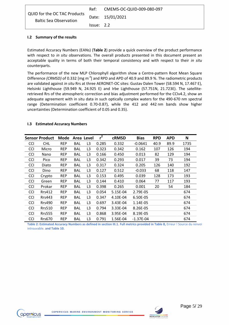
Estimated Accuracy Numbers (EANs) (Table 2) provide a quick overview of the product performance with respect to in situ observations. The overall products presented in this document present an acceptable quality in terms of both their temporal consistency and with respect to their in situ counterparts.

The performance of the new MLP Chlorophyll algorithm show a Centre-pattern Root Mean Square Difference (CRMSD) of 0.332 [mg m-3] and RPD and APD of 40.9 and 89.9 %. The radiometric products are validated against in situ Rrs at three AERONET-OC sites: Gustav Dalen Tower (58.594 N, 17.467 E), Helsinki Lighthouse (59.949 N, 24.925 E) and Irbe Lighthouse (57.751N, 21.723E). The satellite-retrieved Rrs of the atmospheric correction and bias adjustment performed for the CCIv4.2, show an adequate agreement with in situ data in such optically complex waters for the 490-670 nm spectral range (Determination coefficient 0.70-0.87), while the 412 and 442 nm bands show higher uncertainties (Determination coefficient of 0.05 and 0.35).

I.3 Estimated Accuracy Numbers

Sensor Product Mode Area Level r2 cRMSD Bias RPD APD N CCI CHL REP BAL L3 0.285 0.332 -0.0641 40.9 89.9 1735

CCI Micro REP BAL L3 0.323 0.342 0.162 107 126 194

CCI Nano REP BAL L3 0.166 0.450 0.013 82 129 194

CCI Pico REP BAL L3 0.342 0.293 0.017 39 73 194

CCI Diato REP BAL L3 0.317 0.324 0.205 126 140 192

CCI Dino REP BAL L3 0.127 0.512 -0.033 68 118 147

CCI Crypto REP BAL L3 0.153 0.495 0.039 128 173 193

CCI Green REP BAL L3 0.144 0.410 0.064 77 117 193

CCI Prokar REP BAL L3 0.398 0.265 0.001 20 54 184

CCI Rrs412 REP BAL L3 0.054 5.15E-04 2.79E-05 674





CCI Rrs670 REP BAL L3 0.791 1.56E-04 -1.37E-04 674 Table 2: Estimated Accuracy Numbers as defined in section III.1. Full metrics provided in Table 8, Erreur ! Source du renvoi introuvable. and Table 10.




Date: 15/01/2021

Issue: 2.2

Page 6/ 29

II PRODUCTION SYSTEM DESCRIPTION

II.1 Production Centre: Ocean Colour (OC) TAC

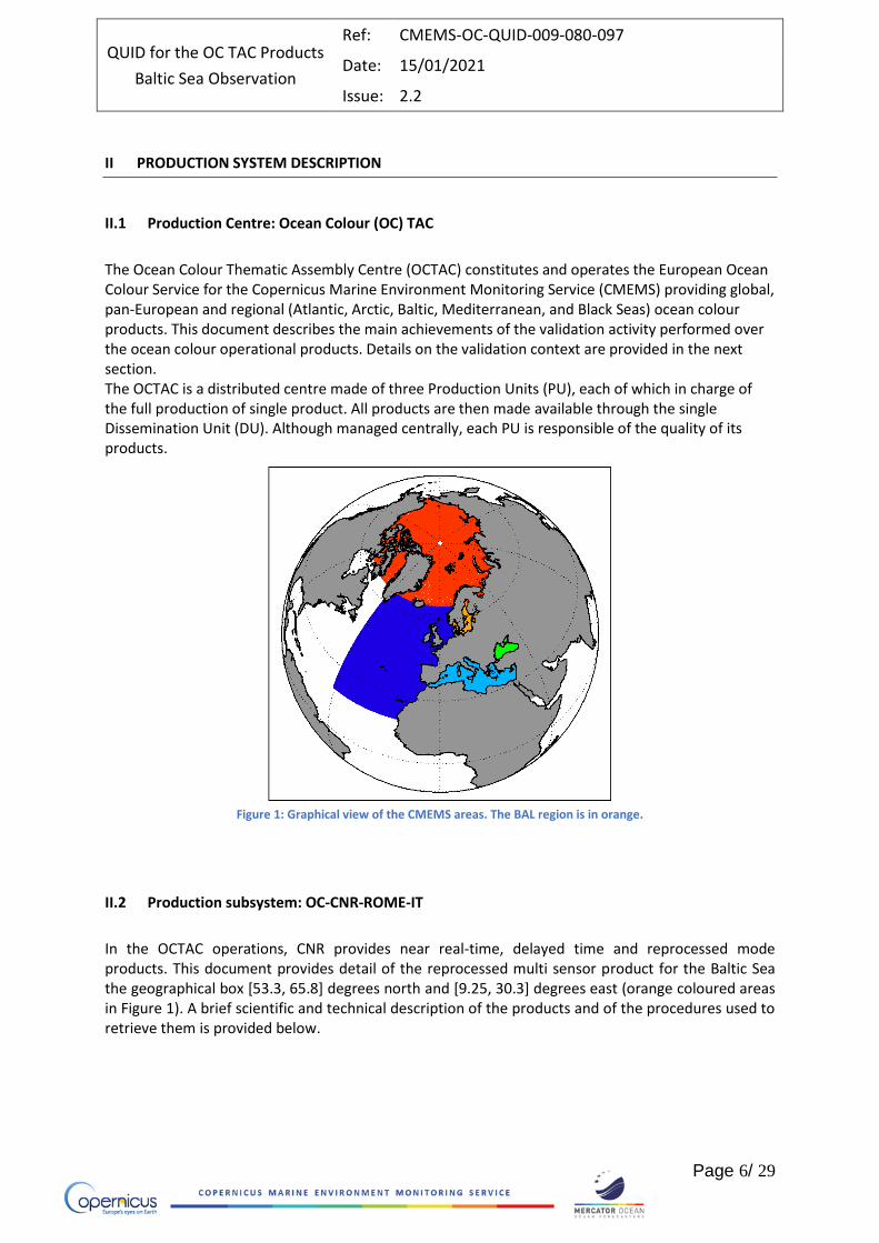
The Ocean Colour Thematic Assembly Centre (OCTAC) constitutes and operates the European Ocean Colour Service for the Copernicus Marine Environment Monitoring Service (CMEMS) providing global, pan-European and regional (Atlantic, Arctic, Baltic, Mediterranean, and Black Seas) ocean colour products. This document describes the main achievements of the validation activity performed over the ocean colour operational products. Details on the validation context are provided in the next section. The OCTAC is a distributed centre made of three Production Units (PU), each of which in charge of the full production of single product. All products are then made available through the single Dissemination Unit (DU). Although managed centrally, each PU is responsible of the quality of its products.

Figure 1: Graphical view of the CMEMS areas. The BAL region is in orange.

II.2 Production subsystem: OC-CNR-ROME-IT

In the OCTAC operations, CNR provides near real-time, delayed time and reprocessed mode products. This document provides detail of the reprocessed multi sensor product for the Baltic Sea the geographical box [53.3, 65.8] degrees north and [9.25, 30.3] degrees east (orange coloured areas in Figure 1). A brief scientific and technical description of the products and of the procedures used to retrieve them is provided below.




Date: 15/01/2021

Issue: 2.2

Page 7/ 29

II.3 Production temporal coverage

The REP archive is regularly updated/extended at least twice year.

II.4 Production chain

This section describes the processing chain for the data production in the Baltic Sea, of reprocessed time series (REP) of surface chlorophyll concentration (CHL). Primary input data are Level-3 (L3) remote-sensing reflectances (Rrs) at ~ 1 km spatial resolution derive from daily L3 the ESA-CCI (Climate Change Initiative). CHL is retrieved by a new MLP algorithm developed for the Baltic Sea and applied to remote sensing reflectances posteriorly adjusted to the automated in situ radiometry collected at two AERONET-OC station with a regression scheme.

II.4.1 Level-3 (L3) remote-sensing reflectances

Rrs spectra are available at six wavebands (bands 412-443-490-510-555-670 nm), as the entire data time series is processed with a consistent configuration, providing users with the longest and most consistent available data time series, spanning over twenty years (1997 to 2018), for the Baltic Sea. Within CMEMS, the spectral Rrs is produced by the Plymouth Marine Laboratory (PML), which uses the OC-CCI processor version 4.2 (www.esa-oceancolour-cci.org) to merge at 1km resolution (rather than at 4km as for OC-CCI) MERIS, MODIS-AQUA, SeaWiFS and VIIRS data. The multisensor strategy responds to IOCCG guidelines, according to which, coverage when three sensors are used could be double that compared with a single sensor product. This might be very helpful in the case of the Baltic Sea, which suffers from high cloud cover.

Atmospheric correction is performed independently for each sensor, and the merging is performed for the calibrated reflectances, after proper band shift to the SeaWiFS bands (Mélin and Sclep, 2015). The dataset used in this version, hereafter referred to as CCIv4, incorporates NASA atmospheric correction and the R2018.0 reprocessing for MODIS-AQUA, SeaWiFS and VIIRS, while MERIS R2012.0 was processed with POLYMER.

II.4.2 Chlorophyll algorithm

II.4.2.1 Previous regional chlorophyll algorithm

In the previous algorithm for the Baltic sea, presented in Pitarch et al. (2016), the algorithm for retrieval of chlorophyll concentration (CHL) from Rrs was a recalibration of the OC4v6 algorithm (Werdell, 2010): log10(CHLBAL)=[log10(CHLOC4v6)-n]/m, with m=0.5884, n=0.3751.

http://www.esa-oceancolour-cci.org/




Date: 15/01/2021

Issue: 2.2

Page 8/ 29

II.4.2.2 New regional chlorophyll algorithm

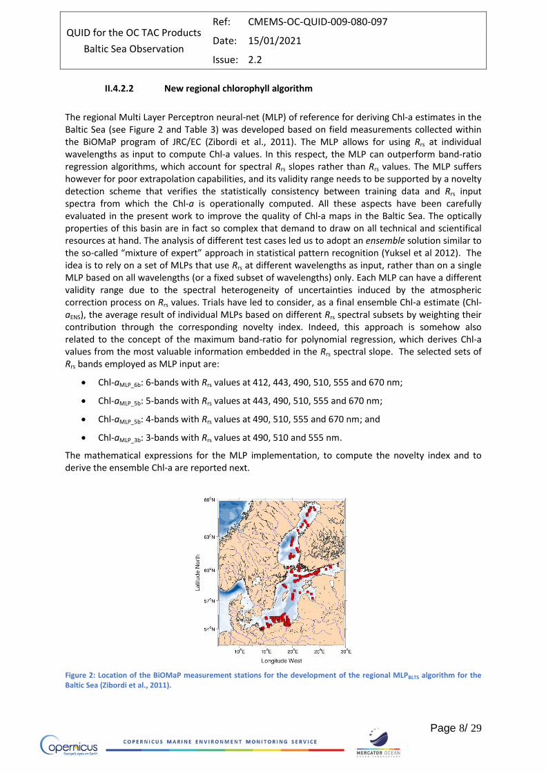
The regional Multi Layer Perceptron neural-net (MLP) of reference for deriving Chl-a estimates in the Baltic Sea (see Figure 2 and Table 3) was developed based on field measurements collected within the BiOMaP program of JRC/EC (Zibordi et al., 2011). The MLP allows for using Rrs at individual wavelengths as input to compute Chl-a values. In this respect, the MLP can outperform band-ratio regression algorithms, which account for spectral Rrs slopes rather than Rrs values. The MLP suffers however for poor extrapolation capabilities, and its validity range needs to be supported by a novelty detection scheme that verifies the statistically consistency between training data and Rrs input spectra from which the Chl-a is operationally computed. All these aspects have been carefully evaluated in the present work to improve the quality of Chl-a maps in the Baltic Sea. The optically properties of this basin are in fact so complex that demand to draw on all technical and scientifical resources at hand. The analysis of different test cases led us to adopt an ensemble solution similar to the so-called “mixture of expert” approach in statistical pattern recognition (Yuksel et al 2012). The idea is to rely on a set of MLPs that use Rrs at different wavelengths as input, rather than on a single MLP based on all wavelengths (or a fixed subset of wavelengths) only. Each MLP can have a different validity range due to the spectral heterogeneity of uncertainties induced by the atmospheric correction process on Rrs values. Trials have led to consider, as a final ensemble Chl-a estimate (Chl-aENS), the average result of individual MLPs based on different Rrs spectral subsets by weighting their contribution through the corresponding novelty index. Indeed, this approach is somehow also related to the concept of the maximum band-ratio for polynomial regression, which derives Chl-a values from the most valuable information embedded in the Rrs spectral slope. The selected sets of Rrs bands employed as MLP input are:

Chl-aMLP_6b: 6-bands with Rrs values at 412, 443, 490, 510, 555 and 670 nm;

Chl-aMLP_5b: 5-bands with Rrs values at 443, 490, 510, 555 and 670 nm;

Chl-aMLP_5b: 4-bands with Rrs values at 490, 510, 555 and 670 nm; and

Chl-aMLP_3b: 3-bands with Rrs values at 490, 510 and 555 nm.

The mathematical expressions for the MLP implementation, to compute the novelty index and to derive the ensemble Chl-a are reported next.

Figure 2: Location of the BiOMaP measurement stations for the development of the regional MLPBLTS algorithm for the Baltic Sea (Zibordi et al., 2011).




Date: 15/01/2021

Issue: 2.2

Page 9/ 29

The MLP scheme

The MLP may be viewed as a practical algorithm for performing a nonlinear input-output mapping of general nature. Computational steps include data pre- and post-processing operations and the definition of applicability range as described next.

Data pre-processing

The input Rrs values at the selected spectral wavelengths are firstly log-transformed l = log10(Rrs), and then z-score scaled x = (l - μl) / σl, where μl and σl indicate respectively the mean and standard deviation (see Table 3) of log-transformed Rrs of the BiOMaP training data (D’Alimonte et al., 2011; D’Alimonte et al., 2014).

The Multi-layer Perceptron scheme

The MLPBLTS scheme consists of successive layers of units, with each unit in one layer connected to each unit of the next layer. Let y=f(x) denote the MLP function, where the input vector x has entries xi for i=1,…,d. The value of the hidden unit j, denoted aj, is a linear combination of the input quantities:

𝑎𝑗 = b𝑗(1)

+ ∑ w𝑗𝑖(1)

𝑥𝑖

𝑑

𝑖=1

where w(1)ji represent the weights linking the input unit i to the hidden unit j, and b(1)

j is the bias adaptive parameter. The activation of the hidden unit j, identified with zj and representing the input for the next layer, is obtained as:

𝑧𝑗 = 𝑔(𝑎𝑗) = 𝑒𝑎𝑗 − 𝑒−𝑎𝑗

𝑒𝑎𝑗 + 𝑒−𝑎𝑗,

with g indicating the hyperbolic tangent activation function. The output y is computed as:

𝑦 = b(2) + ∑ w𝑗(2)

𝑧𝑗

M

𝑖=1

,

where M indicates the number of hidden units with weight w2j and b(2) is the bias coefficient.

Data post-processing

Data post-processing converts the y value into the final result as MLP = 10(𝑦⋅𝜎𝑐+𝜇𝑐), where μc and μc are the mean and the standard deviation of log-transformed Chl-a in situ measurements, respectively.

Novelty index and MLP applicability range

The MLP applicability range has been identified by means of the novelty index η (D’Alimonte et al., 2014) defined as follows

𝜉 = (𝒍 − 𝝁𝜂) ∙ 𝑨𝜂

𝜁 = 𝜉 √𝛾𝜂⁄

𝜂 = ‖𝜁‖ 𝑛𝜆⁄

where: l is the logarithm of Rrs values; 𝝁𝜂 is the mean of l; 𝐀𝜂 and 𝛾𝜂 array are respectively the

eigenvectors and eigenvalues from the Principal Component Analysis (PCA) of l; ‖𝜁‖ is the Euclidean norm of 𝜁; and 𝑛 is the number of selected Rrs wavelengths.




Date: 15/01/2021

Issue: 2.2

Page 10/ 29

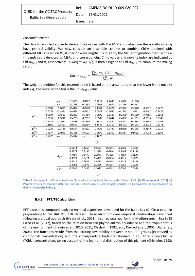
Ensemble scheme

The details reported above to derive Chl-a values with the MLP and determine the novelty index η have general validity. We now consider an ensemble scheme to combine Chl-a obtained with different MLPs based on Rrs at specific wavelengths. To this end, the MLP configuration that use the i-th bands set is denoted as MLPi, and corresponding Chl-a values and novelty index are indicated as Chl-aMLP_i and ηi, respectively. A weight wi= 1/ηi is then assigned to Chl-aMLP_i to compute the mixing result

𝐶ℎ𝑙 − 𝑎𝐸𝑁𝑆 =∑ 𝑤𝑖 ∙𝑁

𝑖=1 𝐶ℎ𝑙 − 𝑎𝑀𝐿𝑃_𝑖

∑ 𝑤𝑖𝑁𝑖=1

.

The weight definition for this ensemble rule is based on the assumption that the lower is the novelty index ηi, the more accredited is the Chl-aMLP_i value.

μl = -3.1603 -3.0312 -2.8155 -2.7409 -2.6652 -3.1614

σl = 0.2588 0.1838 0.1592 0.1607 0.1756 0.2461

w(1) =

-0.7985 0.2080 -0.4472 0.4574 0.4361 -0.1427 -0.3852 0.2818 -0.5851 -0.2278

0.0232 -0.1921 -0.0594 -0.0531 1.0587 -0.2680 -0.2595 1.9991 0.8481 -0.2425

1.0904 0.4620 0.2267 0.5697 0.0892 -0.0123 0.2390 0.7510 0.4695 0.2861

-0.2053 1.6031 0.4763 0.2052 -0.0905 -0.7447 0.4032 -0.1785 0.7916 0.0340

-0.7415 -0.2967 1.0456 0.1586 0.1314 1.0432 0.3897 -0.3688 -0.6143 0.1766

-0.4006 -0.5703 0.0161 0.8207 1.1073 1.0108 0.6197 -0.5683 -0.3330 0.5511

b(1) = 0.9228 −0.0448 0.9684 −0.6415 −0.7833 0.3443 −0.0358 0.1046 −0.3144 −0.2158

w(2)= −0.6977 −1.4963 0.7168 −0.0015 0.5500 −0.6762 0.3854 0.9912 −1.0978 0.1195

b(2) = 0.0222 μc = 0.4514 σc = 0.4222

(a)

𝑨𝜼 =

0.5414 0.4267 -0.6601 0.2885 0.0760 0.0103

0.3879 0.3196 0.1828 -0.6344 -0.5465 -0.1131

0.3491 0.1479 0.3957 -0.1135 0.4552 0.6925

0.3599 0.0411 0.4036 0.0934 0.4515 -0.7023

0.3717 -0.2689 0.3437 0.6198 -0.5226 0.1188

0.4083 -0.7873 -0.3055 -0.3294 0.1069 0.0126

𝜸𝜼 = 0.1902 0.0436 0.0073 0.0013 0.0002 0.0001

(b)

Table 3 Example of coefficients to derive Chl-a values in the Baltic Sea using the 6-bands MLP (D’Alimonte et al., 2011) (a) Parameter sets to compute data pre- and post-processing, as well as MLP weights. (b) Eigenvectors and eigenvalues to define the novelty index η.

II.4.3 PFT/PSC algorithm

PFT dataset is computed applying regional algorithms developed for the Baltic Sea (Di Cicco et al., in preparation) to the BAL REP CHL dataset. These algorithms are empirical relationships developed following a global approach (Hirata et al., 2011), also regionalized for the Mediterranean Sea in Di Cicco et al. (2017), based on the relation between phytoplankton abundance and the trophic status of the environment (Brewin et al., 2010, 2011; Chisholm, 1992; e.g., Devred et al., 2006; Uitz et al., 2006). The functions results from the existing covariability between in situ PFT groups (expressed as chlorophyll concentration) and the corresponding log10‐transformed in situ total chlorophyll a (TChla) concentration, taking account of the log-normal distribution of this pigment (Chisholm, 1992;




Date: 15/01/2021

Issue: 2.2

Page 11/ 29

Hirata et al., 2011). The in-situ pigmental dataset used for the PFT algorithm development in the Black Sea are fully detailed in Section III.1.

PFT in-situ quantification

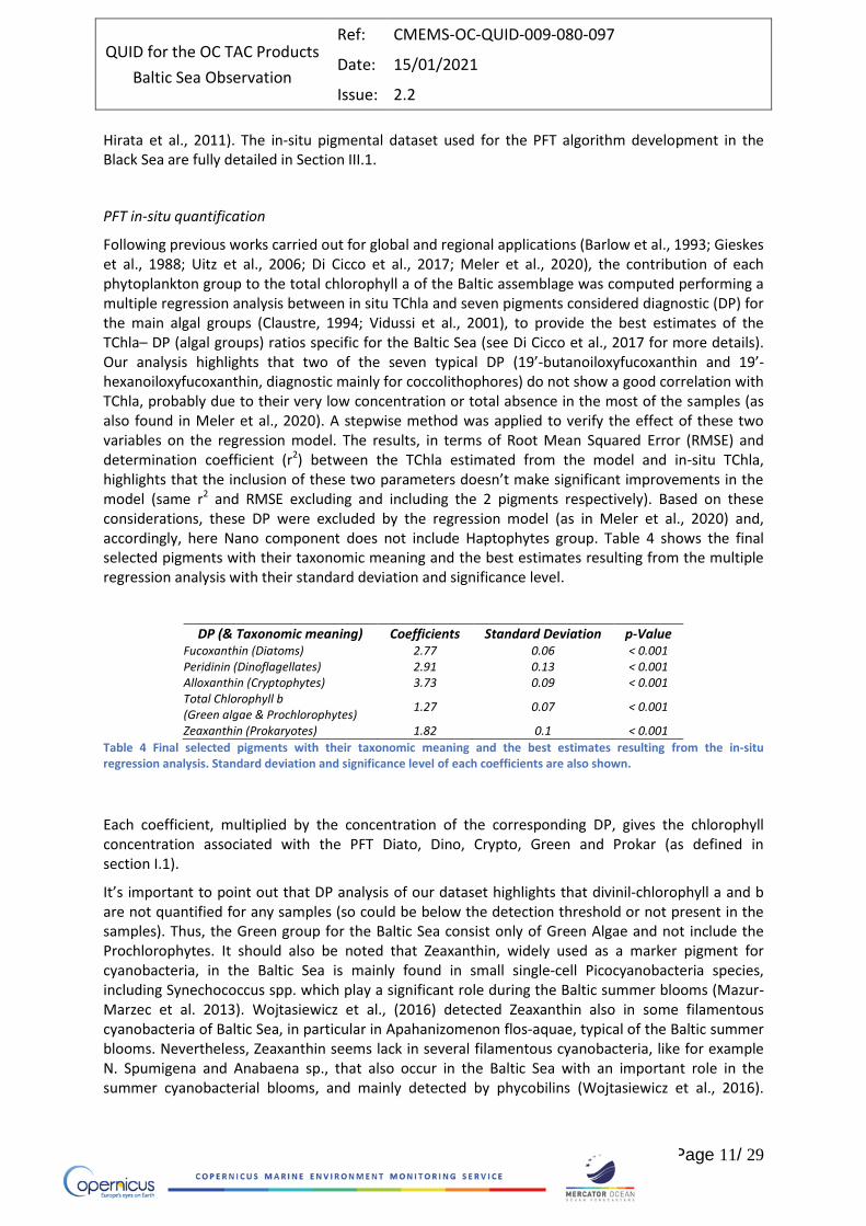
Following previous works carried out for global and regional applications (Barlow et al., 1993; Gieskes et al., 1988; Uitz et al., 2006; Di Cicco et al., 2017; Meler et al., 2020), the contribution of each phytoplankton group to the total chlorophyll a of the Baltic assemblage was computed performing a multiple regression analysis between in situ TChla and seven pigments considered diagnostic (DP) for the main algal groups (Claustre, 1994; Vidussi et al., 2001), to provide the best estimates of the TChla– DP (algal groups) ratios specific for the Baltic Sea (see Di Cicco et al., 2017 for more details). Our analysis highlights that two of the seven typical DP (19’-butanoiloxyfucoxanthin and 19’-hexanoiloxyfucoxanthin, diagnostic mainly for coccolithophores) do not show a good correlation with TChla, probably due to their very low concentration or total absence in the most of the samples (as also found in Meler et al., 2020). A stepwise method was applied to verify the effect of these two variables on the regression model. The results, in terms of Root Mean Squared Error (RMSE) and determination coefficient (r2) between the TChla estimated from the model and in-situ TChla, highlights that the inclusion of these two parameters doesn’t make significant improvements in the model (same r2 and RMSE excluding and including the 2 pigments respectively). Based on these considerations, these DP were excluded by the regression model (as in Meler et al., 2020) and, accordingly, here Nano component does not include Haptophytes group. Table 4 shows the final selected pigments with their taxonomic meaning and the best estimates resulting from the multiple regression analysis with their standard deviation and significance level.

DP (& Taxonomic meaning) Coefficients Standard Deviation p-Value Fucoxanthin (Diatoms) 2.77 0.06 < 0.001 Peridinin (Dinoflagellates) 2.91 0.13 < 0.001 Alloxanthin (Cryptophytes) 3.73 0.09 < 0.001 Total Chlorophyll b (Green algae & Prochlorophytes)

1.27 0.07 < 0.001

Zeaxanthin (Prokaryotes) 1.82 0.1 < 0.001

Table 4 Final selected pigments with their taxonomic meaning and the best estimates resulting from the in-situ regression analysis. Standard deviation and significance level of each coefficients are also shown.

Each coefficient, multiplied by the concentration of the corresponding DP, gives the chlorophyll concentration associated with the PFT Diato, Dino, Crypto, Green and Prokar (as defined in section I.1).

It’s important to point out that DP analysis of our dataset highlights that divinil-chlorophyll a and b are not quantified for any samples (so could be below the detection threshold or not present in the samples). Thus, the Green group for the Baltic Sea consist only of Green Algae and not include the Prochlorophytes. It should also be noted that Zeaxanthin, widely used as a marker pigment for cyanobacteria, in the Baltic Sea is mainly found in small single-cell Picocyanobacteria species, including Synechococcus spp. which play a significant role during the Baltic summer blooms (Mazur-Marzec et al. 2013). Wojtasiewicz et al., (2016) detected Zeaxanthin also in some filamentous cyanobacteria of Baltic Sea, in particular in Apahanizomenon flos-aquae, typical of the Baltic summer blooms. Nevertheless, Zeaxanthin seems lack in several filamentous cyanobacteria, like for example N. Spumigena and Anabaena sp., that also occur in the Baltic Sea with an important role in the summer cyanobacterial blooms, and mainly detected by phycobilins (Wojtasiewicz et al., 2016).




Date: 15/01/2021

Issue: 2.2

Page 12/ 29

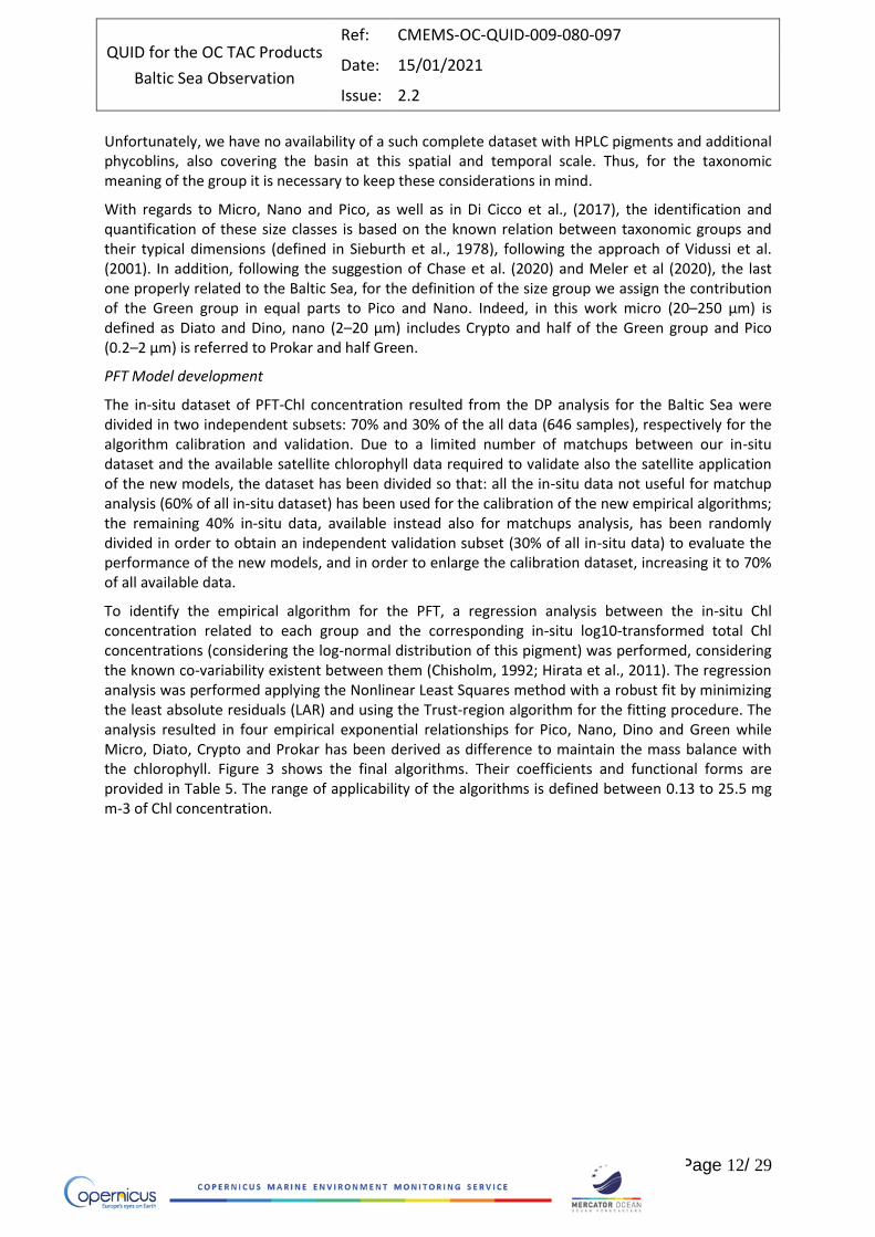
Unfortunately, we have no availability of a such complete dataset with HPLC pigments and additional phycoblins, also covering the basin at this spatial and temporal scale. Thus, for the taxonomic meaning of the group it is necessary to keep these considerations in mind.

With regards to Micro, Nano and Pico, as well as in Di Cicco et al., (2017), the identification and quantification of these size classes is based on the known relation between taxonomic groups and their typical dimensions (defined in Sieburth et al., 1978), following the approach of Vidussi et al. (2001). In addition, following the suggestion of Chase et al. (2020) and Meler et al (2020), the last one properly related to the Baltic Sea, for the definition of the size group we assign the contribution of the Green group in equal parts to Pico and Nano. Indeed, in this work micro (20–250 μm) is defined as Diato and Dino, nano (2–20 μm) includes Crypto and half of the Green group and Pico (0.2–2 μm) is referred to Prokar and half Green.

PFT Model development

The in-situ dataset of PFT-Chl concentration resulted from the DP analysis for the Baltic Sea were divided in two independent subsets: 70% and 30% of the all data (646 samples), respectively for the algorithm calibration and validation. Due to a limited number of matchups between our in-situ dataset and the available satellite chlorophyll data required to validate also the satellite application of the new models, the dataset has been divided so that: all the in-situ data not useful for matchup analysis (60% of all in-situ dataset) has been used for the calibration of the new empirical algorithms; the remaining 40% in-situ data, available instead also for matchups analysis, has been randomly divided in order to obtain an independent validation subset (30% of all in-situ data) to evaluate the performance of the new models, and in order to enlarge the calibration dataset, increasing it to 70% of all available data.

To identify the empirical algorithm for the PFT, a regression analysis between the in-situ Chl concentration related to each group and the corresponding in-situ log10-transformed total Chl concentrations (considering the log-normal distribution of this pigment) was performed, considering the known co-variability existent between them (Chisholm, 1992; Hirata et al., 2011). The regression analysis was performed applying the Nonlinear Least Squares method with a robust fit by minimizing the least absolute residuals (LAR) and using the Trust-region algorithm for the fitting procedure. The analysis resulted in four empirical exponential relationships for Pico, Nano, Dino and Green while Micro, Diato, Crypto and Prokar has been derived as difference to maintain the mass balance with the chlorophyll. Figure 3 shows the final algorithms. Their coefficients and functional forms are provided in Table 5. The range of applicability of the algorithms is defined between 0.13 to 25.5 mg m-3 of Chl concentration.




Date: 15/01/2021

Issue: 2.2

Page 13/ 29

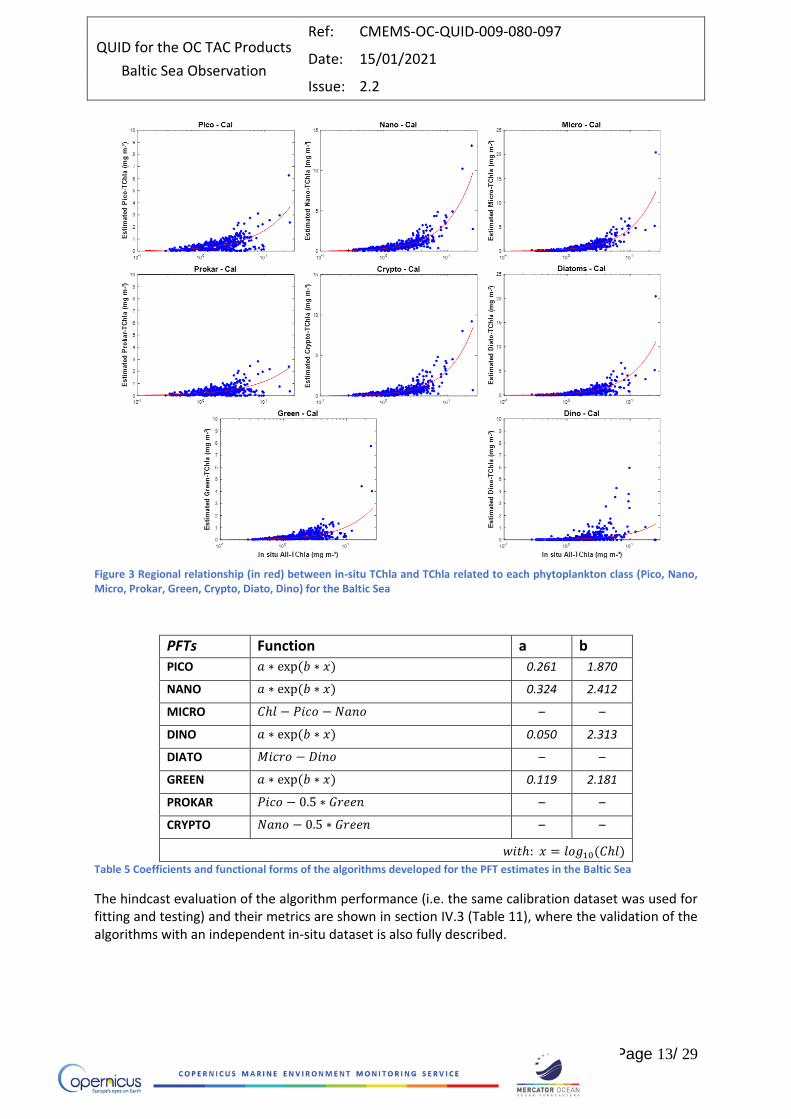
Figure 3 Regional relationship (in red) between in-situ TChla and TChla related to each phytoplankton class (Pico, Nano, Micro, Prokar, Green, Crypto, Diato, Dino) for the Baltic Sea

PFTs Function a b

PICO 𝑎 ∗ exp(𝑏 ∗ 𝑥) 0.261 1.870

NANO 𝑎 ∗ exp(𝑏 ∗ 𝑥) 0.324 2.412

MICRO 𝐶ℎ𝑙 − 𝑃𝑖𝑐𝑜 − 𝑁𝑎𝑛𝑜 – –

DINO 𝑎 ∗ exp(𝑏 ∗ 𝑥) 0.050 2.313

DIATO 𝑀𝑖𝑐𝑟𝑜 − 𝐷𝑖𝑛𝑜 – –

GREEN 𝑎 ∗ exp(𝑏 ∗ 𝑥) 0.119 2.181

PROKAR 𝑃𝑖𝑐𝑜 − 0.5 ∗ 𝐺𝑟𝑒𝑒𝑛 – –

CRYPTO 𝑁𝑎𝑛𝑜 − 0.5 ∗ 𝐺𝑟𝑒𝑒𝑛 – –

𝑤𝑖𝑡ℎ: 𝑥 = 𝑙𝑜𝑔10(𝐶ℎ𝑙) Table 5 Coefficients and functional forms of the algorithms developed for the PFT estimates in the Baltic Sea

The hindcast evaluation of the algorithm performance (i.e. the same calibration dataset was used for fitting and testing) and their metrics are shown in section IV.3 (Table 11), where the validation of the algorithms with an independent in-situ dataset is also fully described.




Date: 15/01/2021

Issue: 2.2

Page 14/ 29

III VALIDATION FRAMEWORK

For this REP product, CNR performs only the offline validation.

III.1 Offline Validation

Offline validation refers to the estimate of the statistical parameters listed in Table 3, based on the pairwise comparison of the satellite estimation (XE)i=1,…,N to the in situ observations (XM)i=1,…,N (whose space-time distribution is shown in Figure 4).

The Baltic Sea is a focal point of activities for protection of the marine environment and is inter-governmentally organized by the Helsinki Commission, HELCOM. In that framework various data are gathered by contracting parties in the COMBINE database, which is hosted by ICES. Amongst others, the database includes chlorophyll-a measurements from the Baltic Sea. This dataset gives a long-time overview of chlorophyll concentrations from the 1970ies to 2017. For this work, the ICES dataset was augmented with the in situ CHL dataset assembled by SYKE based on Alg@line data collected on the Helsinki -Travemunde, Helsinki – Stockholm and Kemi - Travemunde routes from 1997 to 2017. Water samples collected with sequence water sampler from the flow-through water (nominal water inlet 5 m) were filtered with glass fibre filters (Whatman GF F); chlorophyll-a was extracted with ethanol and then chlorophyll content was determined fluorometrically (Kaitala et al., 2008). Satellite CHL was extracted as the median of the 3x3 pixels box around the respective in situ match-up collected between 9-15 local time, (i.e. 10-16 UTC), for a minimum of five valid pixels. The total number of match-ups was 1735.

In-situ Rrs data are Level-2 normalized water-leaving radiances, corrected for bi-directional effects and referred to nadir, taken from automatic and quality controlled measurements at three AERONET-OC sites: Gustav Dalen Tower (58.594 N, 17.467 E), Helsinki Lighthouse (59.949 N, 24.925 E) and Irbe Lighthouse (57.751N, 21.723E). These data were transformed to Rrs and band-shifted to the CCI spectral bands (Mélin and Sclep, 2015) by means of inverse and direct application of the QAA algorithm (Lee et al., 2009). The QAA was modified to warrant anon-negative phytoplankton absorption at any band, which was often the case when applying the QAA as published to the CCI Rrs spectra, often resulting in malfunctioning of the band shift procedure. Output data are provided a few times a day. Eligible match-ups were chosen as the median of all spectra within two hours of the local noon. Match-ups belong to the period 2005-2019.




Date: 15/01/2021

Issue: 2.2

Page 15/ 29

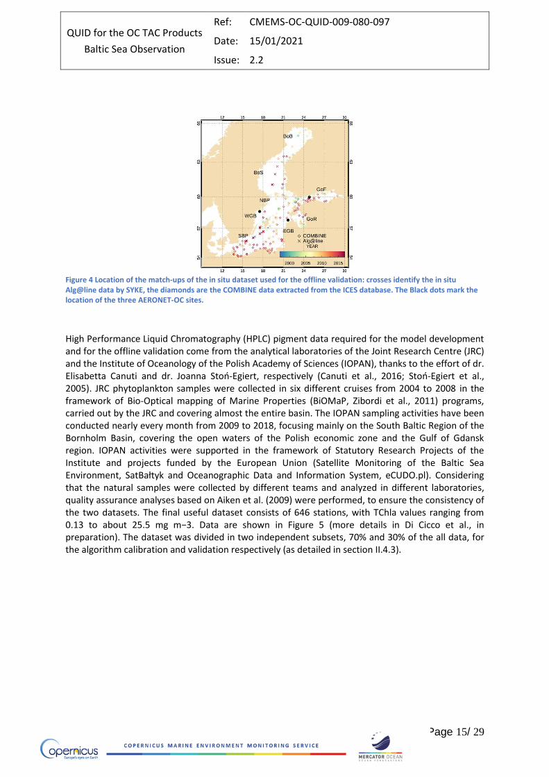
Figure 4 Location of the match-ups of the in situ dataset used for the offline validation: crosses identify the in situ Alg@line data by SYKE, the diamonds are the COMBINE data extracted from the ICES database. The Black dots mark the location of the three AERONET-OC sites.

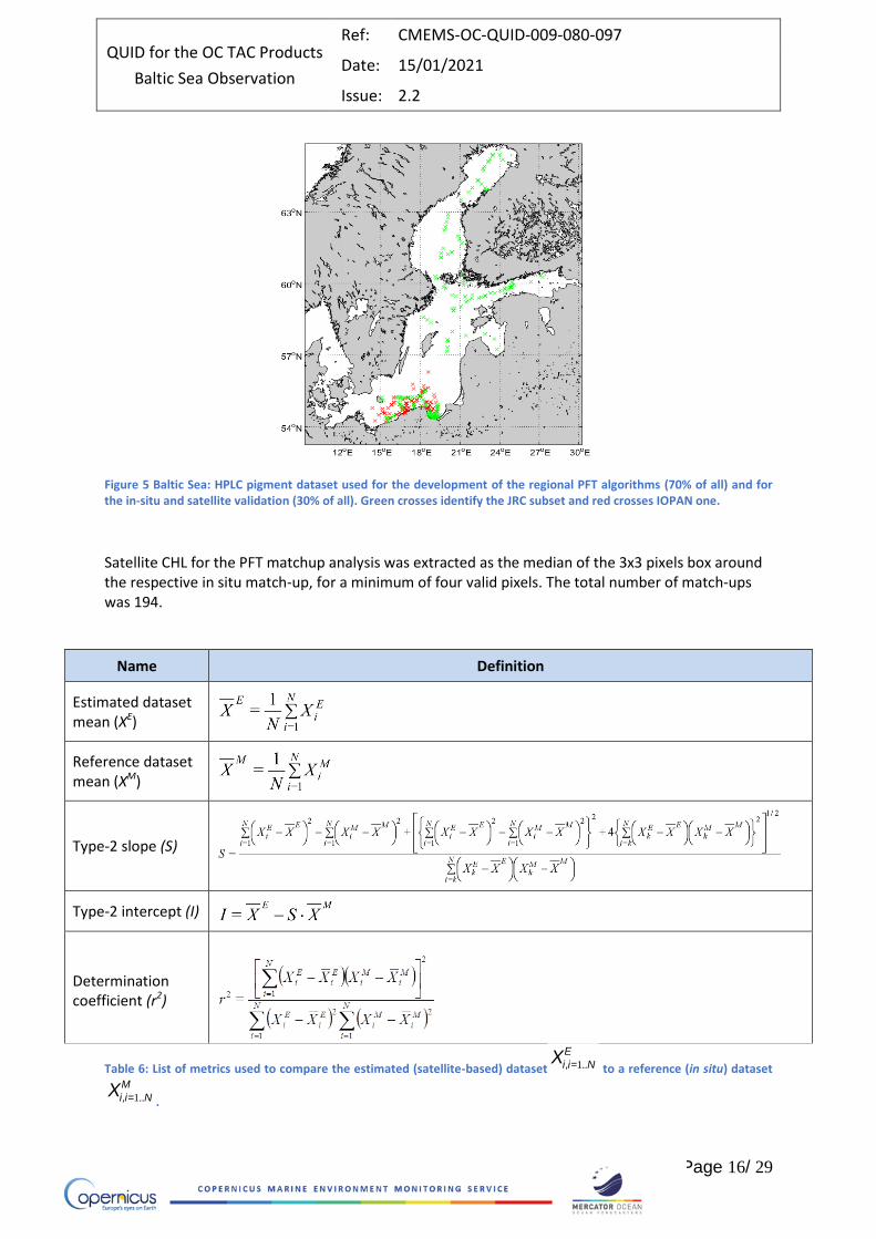
High Performance Liquid Chromatography (HPLC) pigment data required for the model development and for the offline validation come from the analytical laboratories of the Joint Research Centre (JRC) and the Institute of Oceanology of the Polish Academy of Sciences (IOPAN), thanks to the effort of dr. Elisabetta Canuti and dr. Joanna Stoń-Egiert, respectively (Canuti et al., 2016; Stoń-Egiert et al., 2005). JRC phytoplankton samples were collected in six different cruises from 2004 to 2008 in the framework of Bio-Optical mapping of Marine Properties (BiOMaP, Zibordi et al., 2011) programs, carried out by the JRC and covering almost the entire basin. The IOPAN sampling activities have been conducted nearly every month from 2009 to 2018, focusing mainly on the South Baltic Region of the Bornholm Basin, covering the open waters of the Polish economic zone and the Gulf of Gdansk region. IOPAN activities were supported in the framework of Statutory Research Projects of the Institute and projects funded by the European Union (Satellite Monitoring of the Baltic Sea Environment, SatBałtyk and Oceanographic Data and Information System, eCUDO.pl). Considering that the natural samples were collected by different teams and analyzed in different laboratories, quality assurance analyses based on Aiken et al. (2009) were performed, to ensure the consistency of the two datasets. The final useful dataset consists of 646 stations, with TChla values ranging from 0.13 to about 25.5 mg m−3. Data are shown in Figure 5 (more details in Di Cicco et al., in preparation). The dataset was divided in two independent subsets, 70% and 30% of the all data, for the algorithm calibration and validation respectively (as detailed in section II.4.3).




Date: 15/01/2021

Issue: 2.2

Page 16/ 29

Figure 5 Baltic Sea: HPLC pigment dataset used for the development of the regional PFT algorithms (70% of all) and for the in-situ and satellite validation (30% of all). Green crosses identify the JRC subset and red crosses IOPAN one.

Satellite CHL for the PFT matchup analysis was extracted as the median of the 3x3 pixels box around the respective in situ match-up, for a minimum of four valid pixels. The total number of match-ups was 194.

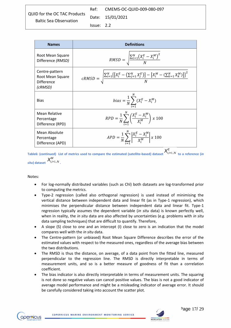
Name Definition

Estimated dataset mean (XE)

Reference dataset mean (XM)

Type-2 slope (S)

Type-2 intercept (I)

Determination coefficient (r2)

Table 6: List of metrics used to compare the estimated (satellite-based) dataset to a reference (in situ) dataset

.

Xi,i=1..N

E

Xi,i=1..N

M




Date: 15/01/2021

Issue: 2.2

Page 17/ 29

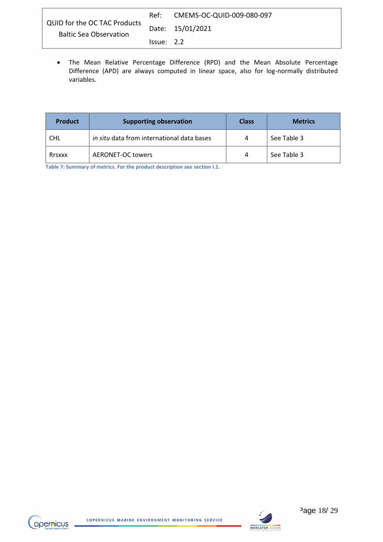
Names Definitions

Root Mean Square Difference (RMSD) 𝑅𝑀𝑆𝐷 = √∑ (𝑋𝑖

𝐸 − 𝑋𝑖𝑀)

2𝑁𝑖=1

𝑁

Centre-pattern Root Mean Square Difference (cRMSD)

𝑐𝑅𝑀𝑆𝐷 = √∑ {[𝑋𝑖

𝐸 − (∑ 𝑋𝑗𝐸𝑁

𝑗=1 )] − [𝑋𝑖𝑀 − (∑ 𝑋𝑘

𝑀𝑁𝑘=1 )]}

2𝑁𝑖=1

𝑁

Bias 𝑏𝑖𝑎𝑠 =1

𝑁∑(𝑋𝑖

𝐸 − 𝑋𝑖𝑀)

𝑁

𝑖=1

Mean Relative Percentage Difference (RPD)

𝑅𝑃𝐷 =1

𝑁∑ (

𝑋𝑖𝐸 − 𝑋𝑖

𝑀

𝑋𝑖𝑀 ) 𝑥 100

𝑁

𝑖=1

Mean Absolute Percentage Difference (APD)

𝐴𝑃𝐷 =1

𝑁∑ |

𝑋𝑖𝐸 − 𝑋𝑖

𝑀

𝑋𝑖𝑀 | 𝑥 100

𝑁

𝑖=1

Table6: (continued) List of metrics used to compare the estimated (satellite-based) dataset to a reference (in

situ) dataset .

Notes:

For log-normally distributed variables (such as Chl) both datasets are log-transformed prior to computing the metrics.

Type-2 regression (called also orthogonal regression) is used instead of minimising the vertical distance between independent data and linear fit (as in Type-1 regression), which minimises the perpendicular distance between independent data and linear fit. Type-1 regression typically assumes the dependent variable (in situ data) is known perfectly well, when in reality, the in situ data are also affected by uncertainties (e.g. problems with in situ data sampling techniques) that are difficult to quantify. Therefore,

A slope (S) close to one and an intercept (I) close to zero is an indication that the model compares well with the in situ data.

The Centre-pattern (or unbiased) Root Mean Square Difference describes the error of the estimated values with respect to the measured ones, regardless of the average bias between the two distributions.

The RMSD is thus the distance, on average, of a data point from the fitted line, measured perpendicular to the regression line. The RMSD is directly interpretable in terms of measurement units, and so is a better measure of goodness of fit than a correlation coefficient.

The bias indicator is also directly interpretable in terms of measurement units. The squaring is not done so negative values can cancel positive values. The bias is not a good indicator of average model performance and might be a misleading indicator of average error. It should be carefully considered taking into account the scatter plot.

Xi,i=1..N

E

Xi,i=1..N

M




Date: 15/01/2021

Issue: 2.2

Page 18/ 29

The Mean Relative Percentage Difference (RPD) and the Mean Absolute Percentage Difference (APD) are always computed in linear space, also for log-normally distributed variables.

Product Supporting observation Class Metrics

CHL in situ data from international data bases 4 See Table 3

Rrsxxx AERONET-OC towers 4 See Table 3

Table 7: Summary of metrics. For the product description see section I.1.




Date: 15/01/2021

Issue: 2.2

Page 19/ 29

IV VALIDATION RESULTS

IV.1 Offline Validation

IV.1.1 Remote Sensing Reflectance

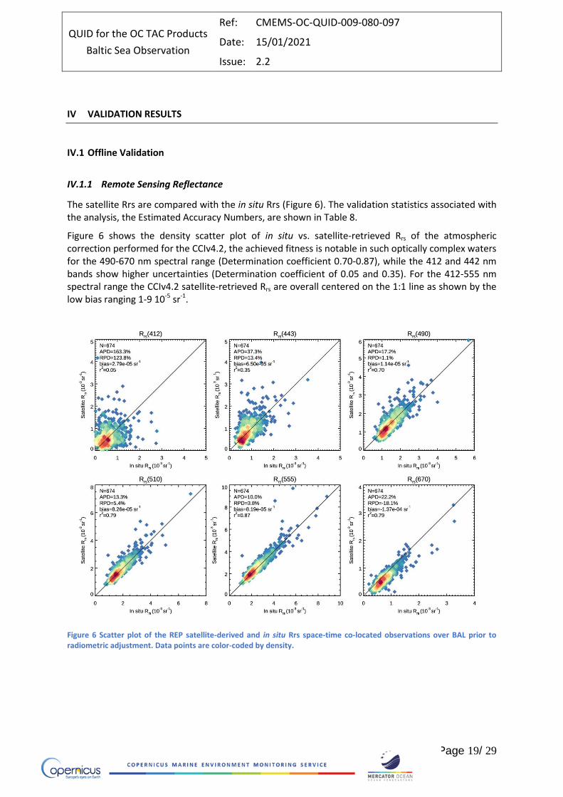
The satellite Rrs are compared with the in situ Rrs (Figure 6). The validation statistics associated with the analysis, the Estimated Accuracy Numbers, are shown in Table 8.

Figure 6 shows the density scatter plot of in situ vs. satellite-retrieved Rrs of the atmospheric correction performed for the CCIv4.2, the achieved fitness is notable in such optically complex waters for the 490-670 nm spectral range (Determination coefficient 0.70-0.87), while the 412 and 442 nm bands show higher uncertainties (Determination coefficient of 0.05 and 0.35). For the 412-555 nm spectral range the CCIv4.2 satellite-retrieved Rrs are overall centered on the 1:1 line as shown by the low bias ranging 1-9 10-5 sr-1.

Figure 6 Scatter plot of the REP satellite-derived and in situ Rrs space-time co-located observations over BAL prior to radiometric adjustment. Data points are color-coded by density.




Date: 15/01/2021

Issue: 2.2

Page 20/ 29

Product XM XE S I r2 RMSD cRMSD Bias RPD APD N

Rrs412 6.11E-4 6.38E-4 1.466 -2.56E-4 0.054 5.16E-4 5.15E-4 2.79E-5 123.8 163.3 674

Rrs443 8.60E-4 9.25E-4 1.464 -3.34E-4 0.347 4.15E-4 4.10E-4 6.50E-5 13.4 37.3 674

Rrs490 1.50E-3 1.51E-3 1.203 -2.93E-4 0.697 3.44E-4 3.43E-4 1.14E-5 1.1 17.2 674

Rrs510 1.86E-3 1.94E-3 1.095 -9.44E-5 0.794 3.43E-4 3.33E-4 8.26E-5 5.4 13.3 674

Rrs555 2.57E-3 2.65E-3 1.064 -8.34E-5 0.868 4.03E-4 3.95E-4 8.19E-5 3.8 10.0 674

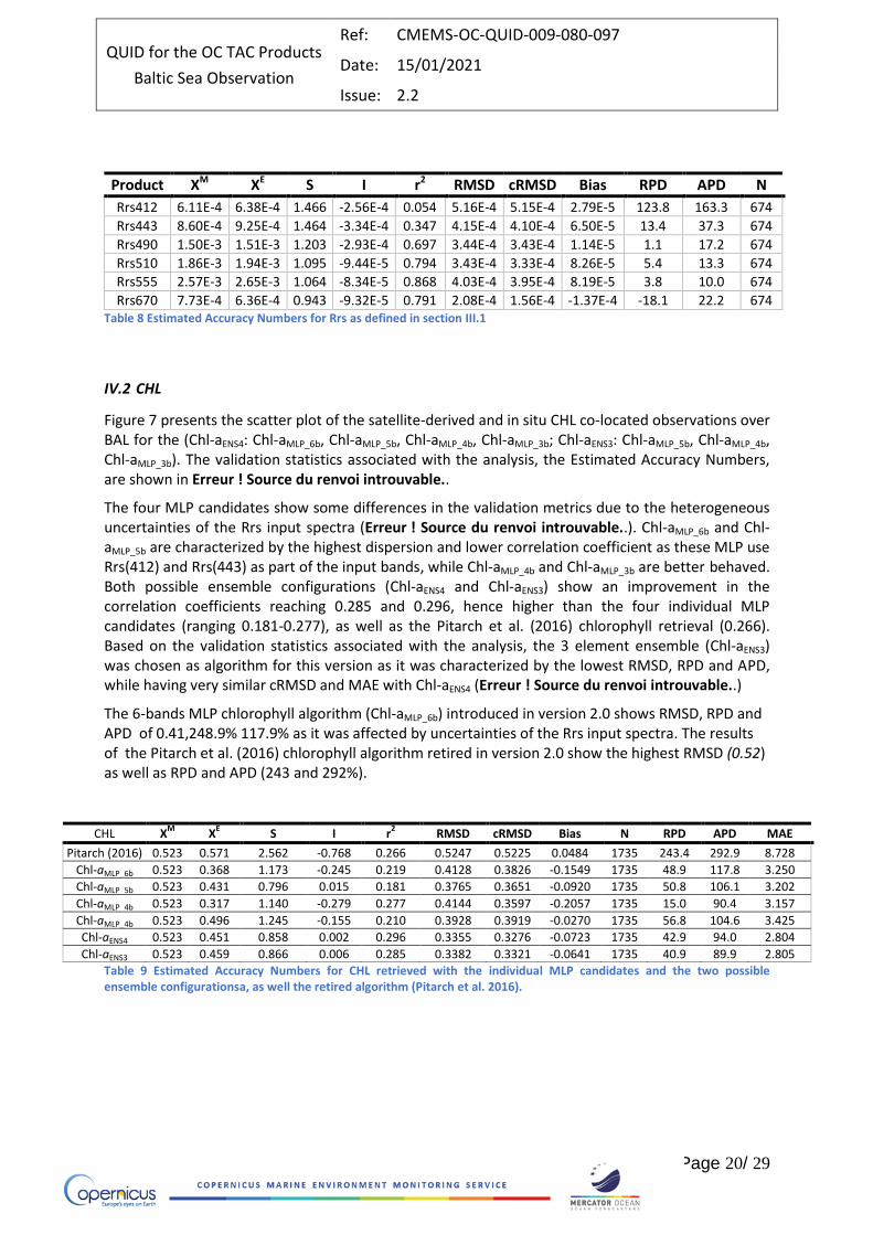
Rrs670 7.73E-4 6.36E-4 0.943 -9.32E-5 0.791 2.08E-4 1.56E-4 -1.37E-4 -18.1 22.2 674 Table 8 Estimated Accuracy Numbers for Rrs as defined in section III.1

IV.2 CHL

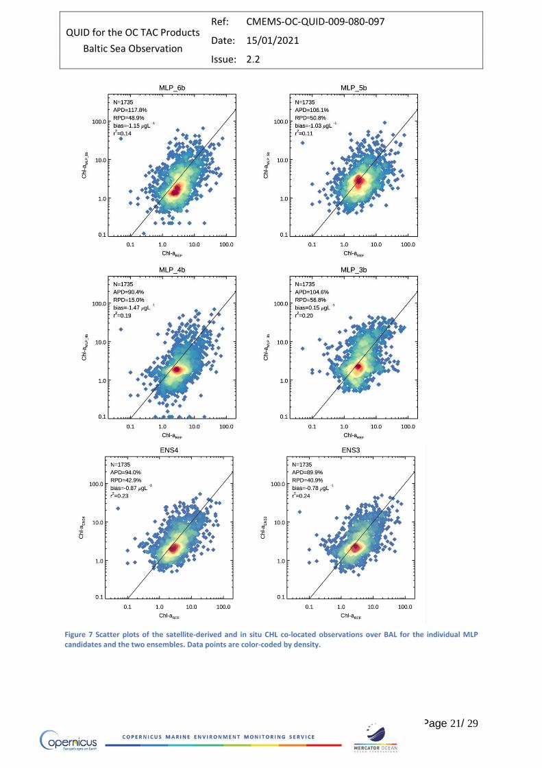
Figure 7 presents the scatter plot of the satellite-derived and in situ CHL co-located observations over BAL for the (Chl-aENS4: Chl-aMLP_6b, Chl-aMLP_5b, Chl-aMLP_4b, Chl-aMLP_3b; Chl-aENS3: Chl-aMLP_5b, Chl-aMLP_4b, Chl-aMLP_3b). The validation statistics associated with the analysis, the Estimated Accuracy Numbers, are shown in Erreur ! Source du renvoi introuvable..

The four MLP candidates show some differences in the validation metrics due to the heterogeneous uncertainties of the Rrs input spectra (Erreur ! Source du renvoi introuvable..). Chl-aMLP_6b and Chl-aMLP_5b are characterized by the highest dispersion and lower correlation coefficient as these MLP use Rrs(412) and Rrs(443) as part of the input bands, while Chl-aMLP_4b and Chl-aMLP_3b are better behaved. Both possible ensemble configurations (Chl-aENS4 and Chl-aENS3) show an improvement in the correlation coefficients reaching 0.285 and 0.296, hence higher than the four individual MLP candidates (ranging 0.181-0.277), as well as the Pitarch et al. (2016) chlorophyll retrieval (0.266). Based on the validation statistics associated with the analysis, the 3 element ensemble (Chl-aENS3) was chosen as algorithm for this version as it was characterized by the lowest RMSD, RPD and APD, while having very similar cRMSD and MAE with Chl-aENS4 (Erreur ! Source du renvoi introuvable..)

The 6-bands MLP chlorophyll algorithm (Chl-aMLP_6b) introduced in version 2.0 shows RMSD, RPD and APD of 0.41,248.9% 117.9% as it was affected by uncertainties of the Rrs input spectra. The results of the Pitarch et al. (2016) chlorophyll algorithm retired in version 2.0 show the highest RMSD (0.52) as well as RPD and APD (243 and 292%).

CHL XM

XE S I r

2 RMSD cRMSD Bias N RPD APD MAE

Pitarch (2016) 0.523 0.571 2.562 -0.768 0.266 0.5247 0.5225 0.0484 1735 243.4 292.9 8.728

Chl-aMLP_6b 0.523 0.368 1.173 -0.245 0.219 0.4128 0.3826 -0.1549 1735 48.9 117.8 3.250

Chl-aMLP_5b 0.523 0.431 0.796 0.015 0.181 0.3765 0.3651 -0.0920 1735 50.8 106.1 3.202

Chl-aMLP_4b 0.523 0.317 1.140 -0.279 0.277 0.4144 0.3597 -0.2057 1735 15.0 90.4 3.157

Chl-aMLP_4b 0.523 0.496 1.245 -0.155 0.210 0.3928 0.3919 -0.0270 1735 56.8 104.6 3.425

Chl-aENS4 0.523 0.451 0.858 0.002 0.296 0.3355 0.3276 -0.0723 1735 42.9 94.0 2.804

Chl-aENS3 0.523 0.459 0.866 0.006 0.285 0.3382 0.3321 -0.0641 1735 40.9 89.9 2.805

Table 9 Estimated Accuracy Numbers for CHL retrieved with the individual MLP candidates and the two possible ensemble configurationsa, as well the retired algorithm (Pitarch et al. 2016).




Date: 15/01/2021

Issue: 2.2

Page 21/ 29

Figure 7 Scatter plots of the satellite-derived and in situ CHL co-located observations over BAL for the individual MLP candidates and the two ensembles. Data points are color-coded by density.




Date: 15/01/2021

Issue: 2.2

Page 22/ 29

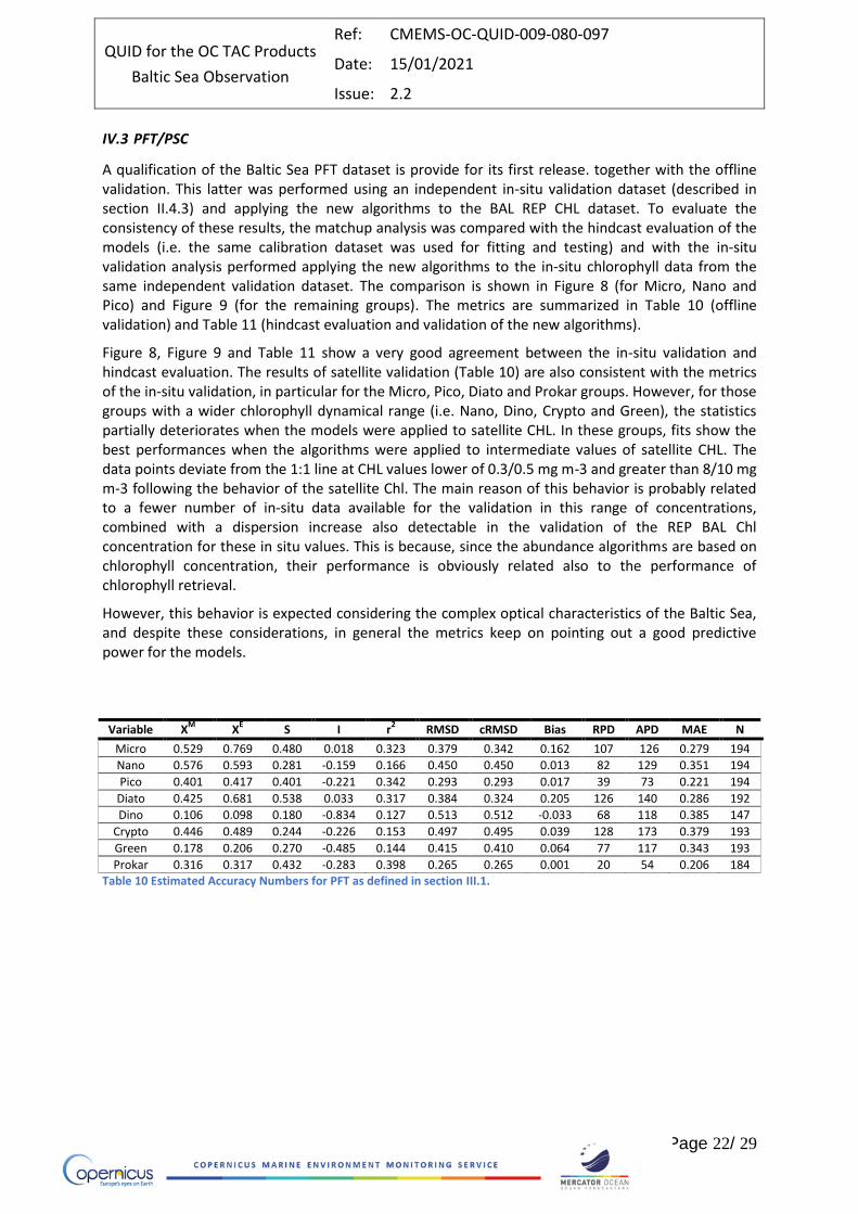
IV.3 PFT/PSC

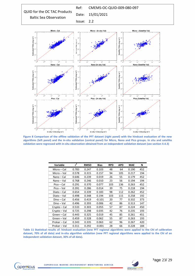
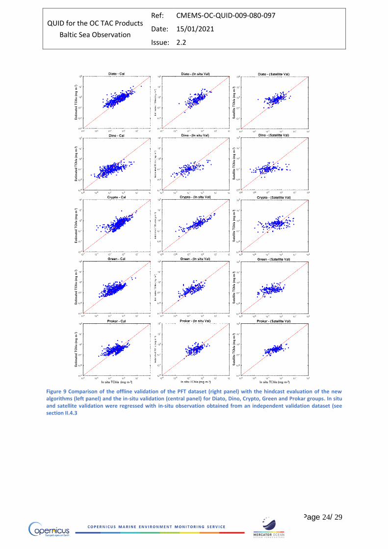
A qualification of the Baltic Sea PFT dataset is provide for its first release. together with the offline validation. This latter was performed using an independent in-situ validation dataset (described in section II.4.3) and applying the new algorithms to the BAL REP CHL dataset. To evaluate the consistency of these results, the matchup analysis was compared with the hindcast evaluation of the models (i.e. the same calibration dataset was used for fitting and testing) and with the in-situ validation analysis performed applying the new algorithms to the in-situ chlorophyll data from the same independent validation dataset. The comparison is shown in Figure 8 (for Micro, Nano and Pico) and Figure 9 (for the remaining groups). The metrics are summarized in Table 10 (offline validation) and Table 11 (hindcast evaluation and validation of the new algorithms).

Figure 8, Figure 9 and Table 11 show a very good agreement between the in-situ validation and hindcast evaluation. The results of satellite validation (Table 10) are also consistent with the metrics of the in-situ validation, in particular for the Micro, Pico, Diato and Prokar groups. However, for those groups with a wider chlorophyll dynamical range (i.e. Nano, Dino, Crypto and Green), the statistics partially deteriorates when the models were applied to satellite CHL. In these groups, fits show the best performances when the algorithms were applied to intermediate values of satellite CHL. The data points deviate from the 1:1 line at CHL values lower of 0.3/0.5 mg m-3 and greater than 8/10 mg m-3 following the behavior of the satellite Chl. The main reason of this behavior is probably related to a fewer number of in-situ data available for the validation in this range of concentrations, combined with a dispersion increase also detectable in the validation of the REP BAL Chl concentration for these in situ values. This is because, since the abundance algorithms are based on chlorophyll concentration, their performance is obviously related also to the performance of chlorophyll retrieval.

However, this behavior is expected considering the complex optical characteristics of the Baltic Sea, and despite these considerations, in general the metrics keep on pointing out a good predictive power for the models.

Variable XM

XE S I r

2 RMSD cRMSD Bias RPD APD MAE N

Micro 0.529 0.769 0.480 0.018 0.323 0.379 0.342 0.162 107 126 0.279 194

Nano 0.576 0.593 0.281 -0.159 0.166 0.450 0.450 0.013 82 129 0.351 194

Pico 0.401 0.417 0.401 -0.221 0.342 0.293 0.293 0.017 39 73 0.221 194

Diato 0.425 0.681 0.538 0.033 0.317 0.384 0.324 0.205 126 140 0.286 192

Dino 0.106 0.098 0.180 -0.834 0.127 0.513 0.512 -0.033 68 118 0.385 147

Crypto 0.446 0.489 0.244 -0.226 0.153 0.497 0.495 0.039 128 173 0.379 193

Green 0.178 0.206 0.270 -0.485 0.144 0.415 0.410 0.064 77 117 0.343 193

Prokar 0.316 0.317 0.432 -0.283 0.398 0.265 0.265 0.001 20 54 0.206 184 Table 10 Estimated Accuracy Numbers for PFT as defined in section ‎III.1.




Date: 15/01/2021

Issue: 2.2

Page 23/ 29

Figure 8 Comparison of the offline validation of the PFT dataset (right panel) with the hindcast evaluation of the new algorithms (left panel) and the in-situ validation (central panel) for Micro, Nano and Pico groups. In situ and satellite validation were regressed with in-situ observation obtained from an independent validation dataset (see section II.4.3)

Variable r2 RMSD Bias RPD APD MAE N

Micro – Cal 0.783 0.247 0.103 48 64 0.190 452

Micro – Val 0.578 0.315 0.157 94 105 0.217 194

Nano – Cal 0.646 0.239 0.019 26 55 0.179 452

Nano – Val 0.768 0.246 0.010 23 56 0.194 194

Pico – Cal 0.291 0.370 0.077 103 136 0.263 452

Pico – Val 0.391 0.286 0.014 39 75 0.218 194

Diato – Cal 0.654 0.339 0.183 98 112 0.262 452

Diato – Val 0.498 0.348 0.194 103 115 0.258 192

Dino – Cal 0.456 0.419 -0.101 20 77 0.332 373

Dino – Val 0.496 0.393 0.006 42 86 0.313 147

Crypto – Cal 0.533 0.303 0.055 57 87 0.224 450

Crypto – Val 0.725 0.298 0.035 42 76 0.235 193

Green – Cal 0.443 0.325 0.019 45 85 0.261 451

Green – Val 0.459 0.328 0.062 55 87 0.263 193

Prokar – Cal 0.343 0.335 0.063 62 96 0.267 420

Prokar – Val 0.311 0.292 -0.001 28 66 0.228 184

Table 11 Statistical results of: hindcast evaluation (new PFT regional algorithms were applied to the Chl of calibration dataset, 70% of all data) and in-situ algorithm validation (new PFT regional algorithms were applied to the Chl of an independent validation dataset, 30% of all data).




Date: 15/01/2021

Issue: 2.2

Page 24/ 29

Figure 9 Comparison of the offline validation of the PFT dataset (right panel) with the hindcast evaluation of the new algorithms (left panel) and the in-situ validation (central panel) for Diato, Dino, Crypto, Green and Prokar groups. In situ and satellite validation were regressed with in-situ observation obtained from an independent validation dataset (see section II.4.3




Date: 15/01/2021

Issue: 2.2

Page 25/ 29

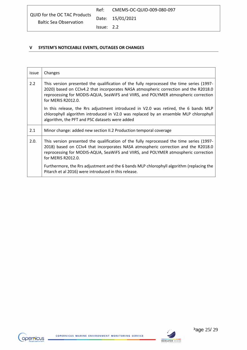
V SYSTEM’S NOTICEABLE EVENTS, OUTAGES OR CHANGES

issue Changes

2.2 This version presented the qualification of the fully reprocessed the time series (1997-2020) based on CCIv4.2 that incorporates NASA atmospheric correction and the R2018.0 reprocessing for MODIS-AQUA, SeaWiFS and VIIRS, and POLYMER atmospheric correction for MERIS R2012.0.

In this release, the Rrs adjustment introduced in V2.0 was retired, the 6 bands MLP chlorophyll algorithm introduced in V2.0 was replaced by an ensemble MLP chlorophyll algorithm, the PFT and PSC datasets were added

2.1 Minor change: added new section II.2 Production temporal coverage

2.0. This version presented the qualification of the fully reprocessed the time series (1997-2018) based on CCIv4 that incorporates NASA atmospheric correction and the R2018.0 reprocessing for MODIS-AQUA, SeaWiFS and VIIRS, and POLYMER atmospheric correction for MERIS R2012.0.

Furthermore, the Rrs adjustment and the 6 bands MLP chlorophyll algorithm (replacing the Pitarch et al 2016) were introduced in this release.




Date: 15/01/2021

Issue: 2.2

Page 26/ 29

VI QUALITY CHANGES SINCE PREVIOUS VERSION

The EAN reported in this version are not directly comparable to the previous version as new in-situ data was used. The 3 element ensemble algorithm (Chl-aENS3) was characterized by the lowest RMSD, RPD and APD (0.338, 40.9% and 89.9%), a marked improvement on the 6-bands MLP chlorophyll algorithm (Chl-aMLP_6b) introduced in version 2.0 (RMSD, RPD and APD of 0.41,248.9% 117.9%) The results of the Pitarch et al. (2016) chlorophyll algorithm retired in version 2.0 show the highest RMSD (0.52) as well as RPD and APD (243 and 292%). .




Date: 15/01/2021

Issue: 2.2

Page 27/ 29

VII REFERENCES

Aiken, J., Pradhan, Y., Barlow, R., Lavender, S., Poulton, A., Holligan, P., Hardman-Mountford, N., 2009. Phytoplankton pigments and functional types in the Atlantic Ocean: A decadal assessment, 1995-2005. Deep-Sea Research II, 56, 899-917

Barlow, R. G., Mantoura, R. F. C., Gough, M. A., Fileman, T. W., 1993. Pigment signatures of the phytoplankton composition in the northeastern Atlantic during the 1990 spring bloom. Deep-Sea Research II, Vol. 40, N. 1-2, 459-477.

Brewin, R. J., Sathyendranath, S., Hirata, T., Lavender, S. J., Barciela, R. M., & Hardman-Mountford, N. J., 2010. A three-component model of phytoplankton size class for the Atlantic Ocean. Ecological Modelling, 221(11), pp. 1472-1483.

Brewin, R. J. W., Devred, E., Sathyendranath, S., Lavender, S. J., and Hardman-Mountford, N. J., 2011. Model of phytoplankton absorption based on three size classes, Appl. Optics, 50, pp. 4353–4364.Chisholm, S. W., 1992. Phytoplankton size. In: Primary Productivity and Biogeochemical Cycles in the Sea. Edited by P.G. Falkowski and A.D. Woodhead. Plenum Press, New York.

Canuti, E., Ras, J., Grung, M., Roettgers, R., Costa Goela, P., & Artuso, F. (2016). HPLC/DAD Intercomparison on Phytoplankton Pigments (HIP-1, HIP-2, HIP-3 and HIP-4).

Chase, A. P., Kramer, S. J., Haëntjens, N., Boss, E. S., Karp‐Boss, L., Edmondson, M., & Graff, J. R. (2020). Evaluation of diagnostic pigments to estimate phytoplankton size classes. Limnology and Oceanography: Methods, 18(10), 570-584.

Chisholm, S. W. (1992). “Phytoplankton size,” in Primary Productivity and Biogeochemical Cycles in the Sea, eds P. G. Falkowski and A. D. Woodhead (New York, NY: Plenum Press), 213–237.

Claustre, H., 1994. The trophic status of various oceanic provinces as revealed bv phytoplankton pigment signatures. Limnology and Oceanography, 39(5), 1206-1210.

D. D’Alimonte, G. Zibordi, and F. Mélin. Statistical Method for Generating Cross-Mission Consistent Normalized Water-Leaving Radiances. IEEE Trans. Geosc. Rem. Sens., 46 (12): 4075–4093, December 2008. doi: 10.1109/TGRS.2008.2001819.

D. D’Alimonte, G. Zibordi, J.-F. Berthon, E. Canuti, and T. Kajiyama. Bio-optical Algorithms for European Seas: Performance and Applicability of Neural-Net Inversion Schemes. Technical Report JRC66326, JRC-IES Scientific and Technical Reports, 2011. URL http://publications.jrc.ec.europa.eu/-repository/handle/111111111/22406.

D. D’Alimonte, G. Zibordi, T. Kajiyama, and J.-F. Berthon. Comparison between MERIS and regional high-level products in European seas. Remote Sensing of Environment, 140: 378–395, 2014. ISSN 0034-4257. doi: 10.1016/j.rse.2013.07.029.

Devred, E., Sathyendranath, S., Stuart, V., Maas, H., Ulloa, O., Platt, T., 2006. A two-component model of phytoplankton absorption in the open ocean: Theory and applications. Journal of Geophysical Research, 111, C03011.

Di Cicco, A., Sammartino, M., Marullo, S. and Santoleri, R., (2017) Regional Empirical Algorithms for an Improved Identification of Phytoplankton Functional Types and Size Classes in the Mediterranean Sea Using Satellite Data. Front. Mar. Sci. 4:126. doi: 10.3389/fmars.2017.00126

http://dx.doi.org/10.1109/TGRS.2008.2001819

http://publications.jrc.ec.europa.eu/repository/handle/111111111/22406

http://publications.jrc.ec.europa.eu/repository/handle/111111111/22406

http://dx.doi.org/10.1016/j.rse.2013.07.029




Date: 15/01/2021

Issue: 2.2

Page 28/ 29

Di Cicco, A., Canuti, E., Stoń-Egiert, J., et al. Regional empirical algorithms for the retrieval of Phytoplankton Functional Types and Size Classes in the Baltic Sea from in-situ and satellite data (in preparation)

Gieskes, W. W. C., Kraay, G. W., Nontji, A., & Setiapermana, D., 1988. Monsoonal alternation of a mixed and a layered structure in the phytoplankton of the euphotic zone of the Banda Sea (Indonesia): A mathematical analysis of algal pigment fingerprints. Netherlands Journal of Sea Research, 22(2), pp. 123-137.

Hirata, T., Hardman-Mountford, N. J., Brewin, R. J. W., Aiken, J., Barlow, R., Suzuki, K., Isada, T., Howell, E., Hashioka, T., Noguchi-Aita, M., Yamanaka, Y., 2011. Synoptic relationships between surface Chlorophyll-a and diagnostic pigments specific to phytoplankton functional types. Biogeosciences, 8(2), 311-327.

Kaitala S, G Zibordi, F Mélin, J Seppälä & P Ylöstalo, 2008. Coastal water monitoring and remote sensing products validation using ferrybox and above-water radiometric measurements. EARSeL eProceedings, 7(1): 75-80

Lee, Z. P., Lubac, B., Werdell, J., and Arnone, R.: An update of the quasi-analytical algorithm (QAA_v5), http://www.ioccg.org/groups/Software_OCA/QAA_v5.pdf, 2009.

Mazur-Marzec H, Sutryk K, Kobos J, Hebel A, Hohlfeld N, Błaszczyk A, Toruńska A, Kaczkowska MJ, Łysiak-Pastuszak E, Kraśniewski W, Jesser I (2013) Occurrence of cyanobacteria and cyanotoxin in the Southern Baltic Proper. Filamentous cyanobacteria versus single-celled picocyanobacteria. Hydrobiologia 701:235–252

Meler, J., Woźniak, S. B., & Stoń-Egiert, J. (2020). Comparison of methods for indirectly estimating the phytoplankton population size structure and their preliminary modifications adapted to the specific conditions of the Baltic Sea. Journal of Marine Systems, 212, 103446.

Mélin, F., and Sclep, G.: Band shifting for ocean color multi-spectral reflectance data, Opt. Express, 23, 2262-2279, 10.1364/OE.23.002262, 2015.

Pitarch, J., Volpe, G., Colella, S., Krasemann, H., and Santoleri, R.: Remote sensing of chlorophyll in the Baltic Sea at basin scale from 1997 to 2012 using merged multi-sensor data, Ocean Sci., 12, 379-389, 10.5194/os-12-379-2016, 2016.

Ocean color chlorophyll (OC) v6: http://oceancolor.gsfc.nasa.gov/REPROCESSING/R2009/ocv6/, 2010.

Sieburth, J. M., Smetacek, V., Lenz, J., 1978. Pelagic ecosystem structure- Heterotrophic compartments of the plankton and their relationship to plankton size fractions Limnology and Oceanography 23, 1256-1263.

Stoń-Egiert, J., & Kosakowska, A. (2005). RP-HPLC determination of phytoplankton pigments—comparison of calibration results for two columns. Marine Biology, 147(1), 251-260.

Uitz, J., H. Claustre, A. Morel, and S. B. Hooker (2006), Vertical distribution of phytoplanton communities in open ocean: An assessment based on surface chlorophyll, J. Geophys. Res., 111, C08005, doi:10.1029/2005JC003207.

Vidussi, F., Claustre, H., Manca, B. B., Luchetta, A., Marty, J. C., 2001. Phytoplankton pigment distribution in relation to upper thermocline circulation in the eastern Mediterranean Sea during winter. Journal of Geophysical Research: Oceans (1978–2012), 106(C9), 19939-19956.

Yuksel, S. E., Wilson, J. N., & Gader, P. D. (2012). Twenty years of mixture of experts. IEEE transactions on neural networks and learning systems, 23(8), 1177-1193.

http://www.ioccg.org/groups/Software_OCA/QAA_v5.pdf

http://oceancolor.gsfc.nasa.gov/REPROCESSING/R2009/ocv6/




Date: 15/01/2021

Issue: 2.2

Page 29/ 29

Wojtasiewicz, B., & Stoń-Egiert, J. (2016). Bio-optical characterization of selected cyanobacteria strains present in marine and freshwater ecosystems. Journal of applied phycology, 28(4), 2299-2314.

G. Zibordi, B. Holben, I. Slutsker, D. Giles, D. D’Alimonte, F. Mélin, J.-F. Berthon, D. Vandemark, H. Feng, G. Schuster, B. E. Fabbri, S. Kaitala, and J. Seppälä. AERONET-OC: A network for the validation of ccean color primary radiometric products. J. Atmos. Oceanic Tech., 26 (8): 1634–1651, 2009. doi: 10.1175/2009JTECHO654.1.

G. Zibordi, J.-F. Berthon, F. Mélin, and D. D’Alimonte. Cross-site consistent in situ measurements for satellite ocean color applications: the BiOMaP radiometric dataset. Remote Sens. Environ., 115 (8): 2104–2115, August 2011. ISSN 0034-4257. doi: 10.1016/j.rse.2011.04.013. URL https://-www.doi.org/10.1016/j.rse.2011.04.013.

http://dx.doi.org/10.1175/2009JTECHO654.1

http://dx.doi.org/10.1016/j.rse.2011.04.013

https://www.doi.org/10.1016/j.rse.2011.04.013

https://www.doi.org/10.1016/j.rse.2011.04.013

Documents

OCEAN COLOUR PRODUCTION CENTRE Baltic Sea ......QUID for the OC TAC Products Baltic Sea Observation Ref: CMEMS-OC-QUID-009-080-097 Date: 15/01/2021 Issue: 2.2 Page 2/ 29 CHANGE RECORD