ORIGINAL ARTICLE

Offer Shai Æ Daniel Rubin

Representing and analysing integrated engineering systemsthrough combinatorial representations

Received: 8 May 2002 / Accepted: 13 December 2002 / Published online: 29 November 2003� Springer-Verlag London Limited 2003

Abstract The current paper introduces a systematicmethod for representing and analysing coupled integratedengineering systems by means of general discrete mathe-matical models, called Combinatorial Representations,that can be conveniently implemented in computers. Thecombinatorial representation of this paper, which is basedon graph theory, was previously shown to be useful inrepresenting engineering systems from different engi-neering domains. Once all of the subsystems of an inte-grated multidisciplinary system are brought up to thecommon level of the combinatorial representation, theycease to be separated from one another and the analysisprocess is applied to all of the engineering elements dis-regarding the domain to which they belong.

During the development of the representation andstudy of its inherent properties, special attention wasdedicated to developing an efficient analysis method. Avectorial extension of the mixed variable method knownfrom electrical network theory was found to be the mostsuitable choice for this purpose.

In the paper, the approach is implemented by repre-senting and analysing two systems: one that is a macrosystem comprised of truss, dynamic and electric elements,and another that is a comb-driven micro-resonator. Thetechniques presented in the paper are not limited toanalysis only, but can be applied to many other aspects ofengineering research. Among them is a systematic deri-vation of new ways of presenting engineering elements,one of which – the process of derivation of a new type offorce representation entitled ‘‘face force’’ – is described inthe paper.

Keywords Combinatorial representations Æ Integratedengineering systems Æ Graph theory Æ Mixed variablemethod

Abbreviations

CR Combinatorial RepresentationsFCFS Flow Controlled Flow SourceFCPS Flow Controlled Potential difference SourceFGR Flow Graph RepresentationMCA Multidisciplinary Combinatorial ApproachPCFS Potential difference Controlled Flow SourcePCPS Potential difference Controlled Potential dif-

ference SourcePGR Potential Graph RepresentationRGR Resistance Graph Representation

Other nomenclature

~B Vector circuit matrixbi Damping factor of the damper iCD Chords of GD

C�F Chords of GF excluding independent sourcesCi Capacity of capacitor iCij Initial capacity between combs of transducer

ijcircuit(i) Circuit defined by chord i of the graphcsa cosaÆsinacutset(i) Cutset defined by branch i of the spanning

treedij Gap between the fingers of opposite combs

in transducer ij~DðeÞ Potential difference of edge eDD Set of independent potential difference

sources~D Vector of potential differencesEF Set of edges of graph GF

ED Set of edges of graph GD

~FðeÞ Flow in edge e~F Vector of flowsGF Graph whose independent variables are

flowsGi Stiffness coefficient of rod iGR Resistance graph

Engineering with Computers (2004) 19: 221–232DOI 10.1007/s00366-003-0262-2

O. Shai (&) Æ D. RubinDepartment of Mechanics, Materials and Systems,Faculty of Engineering, Tel-Aviv University,69978 Tel Aviv, IsraelE-mail: shai@eng.tau.ac.ilFax: +972-3-6407617

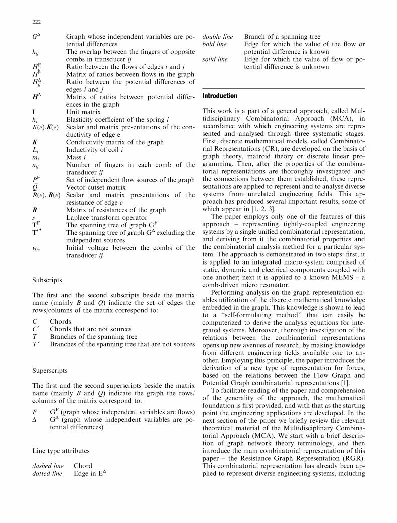
GD Graph whose independent variables are po-tential differences

hij The overlap between the fingers of oppositecombs in transducer ij

HFij Ratio between the flows of edges i and j

HF Matrix of ratios between flows in the graphHD

ij Ratio between the potential differences ofedges i and j

HD Matrix of ratios between potential differ-ences in the graph

I Unit matrixki Elasticity coefficient of the spring iK(e),K(e) Scalar and matrix presentations of the con-

ductivity of edge eK Conductivity matrix of the graphLi Inductivity of coil imi Mass inij Number of fingers in each comb of the

transducer ijPF Set of independent flow sources of the graph~Q Vector cutset matrixR(e), R(e) Scalar and matrix presentations of the

resistance of edge eR Matrix of resistances of the graphs Laplace transform operatorTF The spanning tree of graph GF

T0D

The spanning tree of graph GD excluding theindependent sources

v0ij Initial voltage between the combs of thetransducer ij

Subscripts

The first and the second subscripts beside the matrixname (mainly B and Q) indicate the set of edges therows/columns of the matrix correspond to:

C ChordsC¢ Chords that are not sourcesT Branches of the spanning treeT ¢ Branches of the spanning tree that are not sources

Superscripts

The first and the second superscripts beside the matrixname (mainly B and Q) indicate the graph the rows/columns of the matrix correspond to:

F GF (graph whose independent variables are flows)D GD (graph whose independent variables are po-

tential differences)

Line type attributes

dashed line Chorddotted line Edge in ED

double line Branch of a spanning treebold line Edge for which the value of the flow or

potential difference is knownsolid line Edge for which the value of flow or po-

tential difference is unknown

Introduction

This work is a part of a general approach, called Mul-tidisciplinary Combinatorial Approach (MCA), inaccordance with which engineering systems are repre-sented and analysed through three systematic stages.First, discrete mathematical models, called Combinato-rial Representations (CR), are developed on the basis ofgraph theory, matroid theory or discrete linear pro-gramming. Then, after the properties of the combina-torial representations are thoroughly investigated andthe connections between them established, these repre-sentations are applied to represent and to analyse diversesystems from unrelated engineering fields. This ap-proach has produced several important results, some ofwhich appear in [1, 2, 3].

The paper employs only one of the features of thisapproach – representing tightly-coupled engineeringsystems by a single unified combinatorial representation,and deriving from it the combinatorial properties andthe combinatorial analysis method for a particular sys-tem. The approach is demonstrated in two steps: first, itis applied to an integrated macro-system comprised ofstatic, dynamic and electrical components coupled withone another; next it is applied to a known MEMS – acomb-driven micro resonator.

Performing analysis on the graph representation en-ables utilization of the discrete mathematical knowledgeembedded in the graph. This knowledge is shown to leadto a ‘‘self-formulating method’’ that can easily becomputerized to derive the analysis equations for inte-grated systems. Moreover, thorough investigation of therelations between the combinatorial representationsopens up new avenues of research, by making knowledgefrom different engineering fields available one to an-other. Employing this principle, the paper introduces thederivation of a new type of representation for forces,based on the relations between the Flow Graph andPotential Graph combinatorial representations [1].

To facilitate reading of the paper and comprehensionof the generality of the approach, the mathematicalfoundation is first provided, and with that as the startingpoint the engineering applications are developed. In thenext section of the paper we briefly review the relevanttheoretical material of the Multidisciplinary Combina-torial Approach (MCA). We start with a brief descrip-tion of graph network theory terminology, and thenintroduce the main combinatorial representation of thispaper – the Resistance Graph Representation (RGR).This combinatorial representation has already been ap-plied to represent diverse engineering systems, including

222

multidimensional trusses [4], dynamical systems [2],electrical systems [2].

In the section after that we introduce the vectormixed-variable method, which is the extension to mul-tiple dimensions of the mixed variable method known inelectrical network theory. Then, on the basis of thecombinatorial properties embedded in the ResistanceGraph Representation (RGR), the analysis procedure isdeveloped.

The next section employs the fact that the ResistanceGraph Representation (RGR) is a general combinatorialrepresentation by which systems from various engineer-ing fields can be represented. Therefore, integrated engi-neering systems consisting of elements from these fieldscan be represented by the Resistance Graph Represen-tation. Analysis based on the vector mixed-variablemethod procedure is then performed in a unified wayupon the Resistance Graph that represents an integratedsystem. In order to facilitate the explanation, the pro-posed method is first demonstrated on a macro-inte-grated engineering system. Afterwards, the method isapplied to MEMS, by representing a comb-driven micro-resonator by the Resistance Graph Representation andderiving the characteristic equations in a systematic way.

Leading on from this, we then have a section whichhighlights the fact that representing integrated systemsby combinatorial representations is not limited only tomodelling and analysing integrated engineering systems,but is also useful in other applications. In this section weintroduce the derivation of a new engineering entityentitled the ‘‘face force’’, which enables one to obtain anew insight on the flow of the forces in structures, and socan reveal special properties inherent in an integratedsystem.

The mathematical foundation of the paper lies ingraph theory, which is a well-known topic in discretemathematics. This issue is widely-used in engineering,especially for analysis of electrical networks [5]. In 1955,Trent [6] was one of the first to establish a relationshipbetween physical systems and graph theory, and sincethen it has been applied to many engineering fields. An-drews has developed a methodology for applying graphsto multidimensional dynamic systems [7, 8]. In structuralmechanics two of the most significant works are by Fen-ves and Branin [9] and Kaveh [10]. In machine theory, thegraph representation, in addition to analysis of mecha-nisms [11], was used as an abstract model of kinematicchains to aid in the creative stage of mechanism design[12]. In simulation, a technique at the level of the com-position of system components has been developed [13].Analogy, on the basis of graph theory, between differentone-dimensional systems such as dynamics, electricity,and heat transfer appears in many books [14, 15].

Methods aimed at unified analysis of systems com-posed of elements from different engineering disciplinesare mainly based on the idea of transforming all of theelements to equivalent elements from only one discipline.One of the earlier works concerning this issue was con-ducted by Kron [16], who approached it by transforming

all of the engineering systems to equivalent electricalcircuits. More recent work has been conducted by Sent-uria who suggested transforming elements in macro-models of MEMS to equivalent electrical elements uponwhich both analysis and design are then performed [17].

Network graphs

The combinatorial representation that is used in thispaper is based on network and graph theories, the rel-evant details of which can be found in [2], or in books ongraph theory, such as [18].

Before approaching the combinatorial representationitself, a brief review of the definitions specific to theMultidisciplinary Combinatorial Approach (MCA) isneeded. The paper uses terms from network theorywhere graphs are usually characterized by matrices suchas cutset, circuit and incidence matrices [19]. In thecurrent approach, graphs are used to represent both thetopology and the geometry of the engineering system, sothe matrices are resolved into two corresponding types:vector matrices and scalar matrices [2]. The first type isactually the type of matrix that is used in network theory[19], where the term ‘‘vector’’ stands for the fact thatthese matrices provide information about the topologi-cal relations of the vectors of the network variables,without considering their geometry. The matrices of thesecond type – scalar – provide information about thegeometry of the corresponding engineering elements.These matrices can be obtained from the vector matricesby multiplying each of their columns by a unit vector inthe direction of the corresponding engineering element.The above definitions were found to be useful, since theyhelp to reveal both topological and geometrical prop-erties embedded in graphs.

There are several graph representations that are usedfor representing various engineering systems in theMultidisciplinary Combinatorial Approach (MCA) [2].The combinatorial representation that is employed inthis paper is the Resistance Graph Representation(RGR); therefore its underlying theory and propertiesare provided in the following subsection.

Resistance graph

The resistance graph, designated GR, is a networkgraph, where in certain edges there is a dependence be-tween flow and potential difference. Additionally, theflows and the potential differences in the resistancegraph must satisfy two general laws: the flow law forflows and potential law for potential differences.

– Flow Law: the vector sum of the flows in every cutsetof GR is equal to zero.

The matrix form of the Flow Law is:

~Q �~F¼0 ð1Þ

223

where ~F is the flow vector and ~Q is the vector cutsetmatrix.

– Potential Law: for every circuit in GR, the sum of thepotential differences of all the circuit edges is equal tozero.

In matrix representation, this law is written:

~B �~D ¼ 0 ð2Þ

where ~D is the potential difference vector and ~B is thevector circuit matrix.

One of the main properties of this representation isthe orthogonality principle:

~B � ~Qt ¼ 0 ð3Þ

Several important relations between the matricesand the graph variables, namely the flows and thepotential differences, can be derived from the orthog-onality principle and the flow and potential laws, asfollows:

~BT ¼ �~QtC ð4Þ

~D ¼ ~Qt �~DT ð5Þ

~F ¼ ~Bt �~FC ð6Þ

where the subscripts T and C indicate that the cor-responding matrix (vector) includes only the columns(members) corresponding to the branches of the treeand the chords respectively.

The edges of the graph are classified in accordancewith the relations between their flows and potentialdifferences into four types of edges:

– resistance edges– flow source edges

– potential difference source edges– two-port edges

The definitions of these four types follow.Resistance edges are edges where the dependence be-

tween the flow and potential difference is characterizedby either a constant scalar (Eq. 7) or a constant matrix(Eq. 8), as follows:

~DðeÞ���

��� ¼ RðeÞ � ~F ðeÞ

��

��; ~F ðeÞ

��

�� ¼ KðeÞ � ~DðeÞ

���

��� ð7Þ

~D eð Þ ¼ R eð Þ �~F eð Þ; ~F ðeÞ ¼ KðeÞ �~DðeÞ ð8Þ

where ~DðeÞ and ~F ðeÞ are the potential difference and theflow of edge e.

Flow source edges are edges in which the flow is givenand is independent of the potential difference in the edge.

Potential difference source edges are edges in whichthe potential difference is given and is independent of theflow in the edge.

Two-ports are the elements that contain two edges inthe resistance graph.

The four variables possessed by the two edges aredesignated ~D1;~D2;~F1;~F2. The two-port defines variousmathematical relations between the pairs of these vari-ables. In most cases, in accordance with these connec-tions, the variables of one of the edges are determined bythe variables of the other; so the former edge can bereferred to as the ‘‘source edge’’ and the latter as the‘‘control edge’’. The mathematical connections betweenthe variables are expressed by terminal equations writtenin the form of matrix-vector multiplications.

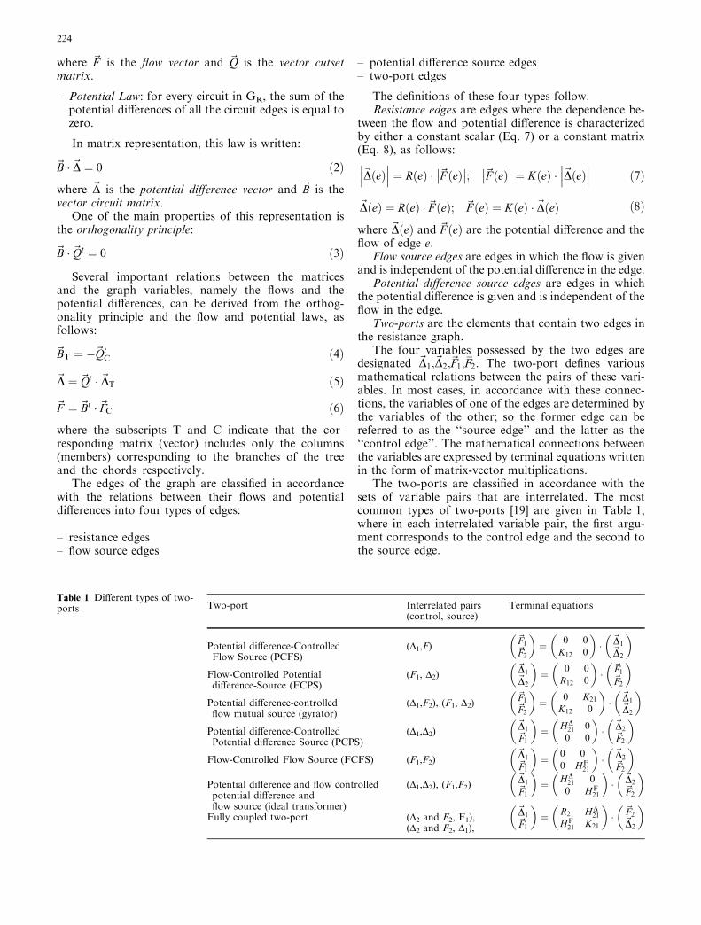
The two-ports are classified in accordance with thesets of variable pairs that are interrelated. The mostcommon types of two-ports [19] are given in Table 1,where in each interrelated variable pair, the first argu-ment corresponds to the control edge and the second tothe source edge.

Table 1 Different types of two-ports Two-port Interrelated pairs

(control, source)Terminal equations

Potential difference-ControlledFlow Source (PCFS)

(D1,F)~F1~F2

� �

¼ 0 0K12 0

� �

�~D1~D2

� �

Flow-Controlled Potentialdifference-Source (FCPS)

(F1, D2)~D1~D2

� �

¼ 0 0R12 0

� �

�~F1~F2

� �

Potential difference-controlledflow mutual source (gyrator)

(D1,F2), (F1, D2)~F1~F2

� �

¼ 0 K21

K12 0

� �

�~D1~D2

� �

Potential difference-ControlledPotential difference Source (PCPS)

(D1,D2)~D1~F1

� �

¼ HD21 00 0

� �

�~D2~F2

� �

Flow-Controlled Flow Source (FCFS) (F1,F2)~D1~F1

� �

¼ 0 00 HF

21

� �

�~D2~F2

� �

Potential difference and flow controlledpotential difference andflow source (ideal transformer)

(D1,D2), (F1,F2)~D1~F1

� �

¼ HD21 00 HF

21

� �

�~D2~F2

� �

Fully coupled two-port (D2 and F2, F1),~D1~F1

� �

¼ R21 HD21

HF21 K21

� �

�~F2~D2

� �

(D2 and F2, D1),

224

Self-formulating method for obtaining the analysisequations for the Resistance Graph Representation

The mixed variable method is a well-known methodwidely used in electrical network theory [19]. In thismethod, the independent variables (main unknowns) arechosen to be partially potential differences and partiallyflows. After finding these independent unknowns, all ofthe flows and all of the potential differences of the graphcan be easily determined. This section introduces avectorial extension of this method, where the variablesare vectors, in contrast to the scalars in electrical theory.In order to distinguish this extension from the originalmethod, it will be referred as the vectorial mixed variablemethod. The mathematical derivation of the methodfollows.

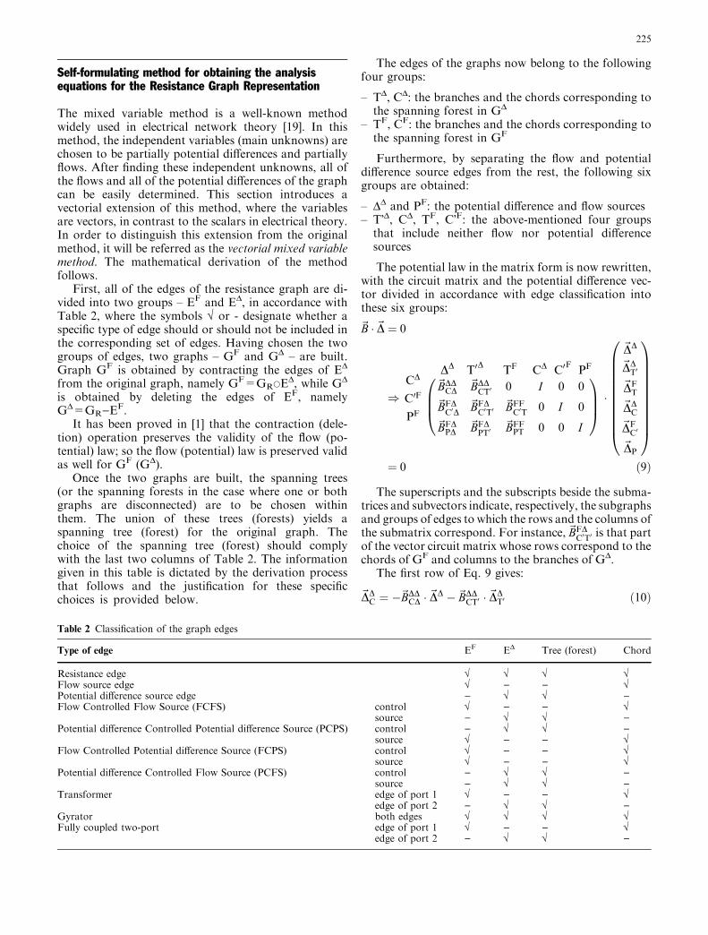
First, all of the edges of the resistance graph are di-vided into two groups – EF and ED, in accordance withTable 2, where the symbols � or - designate whether aspecific type of edge should or should not be included inthe corresponding set of edges. Having chosen the twogroups of edges, two graphs – GF and GD – are built.Graph GF is obtained by contracting the edges of ED

from the original graph, namely GF=GRsED, while GD

is obtained by deleting the edges of EF, namelyGD=GR)EF.

It has been proved in [1] that the contraction (dele-tion) operation preserves the validity of the flow (po-tential) law; so the flow (potential) law is preserved validas well for GF (GD).

Once the two graphs are built, the spanning trees(or the spanning forests in the case where one or bothgraphs are disconnected) are to be chosen withinthem. The union of these trees (forests) yields aspanning tree (forest) for the original graph. Thechoice of the spanning tree (forest) should complywith the last two columns of Table 2. The informationgiven in this table is dictated by the derivation processthat follows and the justification for these specificchoices is provided below.

The edges of the graphs now belong to the followingfour groups:

– TD, CD: the branches and the chords corresponding tothe spanning forest in GD

– TF, CF: the branches and the chords corresponding tothe spanning forest in GF

Furthermore, by separating the flow and potentialdifference source edges from the rest, the following sixgroups are obtained:

– DD and PF: the potential difference and flow sources– T�D, CD, TF, C�F: the above-mentioned four groups

that include neither flow nor potential differencesources

The potential law in the matrix form is now rewritten,with the circuit matrix and the potential difference vec-tor divided in accordance with edge classification intothese six groups:

~B �~D ¼ 0

)CD

C0F

PF

DD T0D

TF CD C0F

PF

~BDDCD

~BDDCT0 0 I 0 0

~BFDC0D

~BFDC0T0

~BFFC0T

0 I 0

~BFDPD

~BFDPT0

~BFFPT 0 0 I

0

BB@

1

CCA

�

~DD

~DDT0

~DFT

~DDC

~DFC0

~DP

0

BBBBBBBBBB@

1

CCCCCCCCCCA

¼ 0 ð9Þ

The superscripts and the subscripts beside the subma-trices and subvectors indicate, respectively, the subgraphsand groups of edges to which the rows and the columns ofthe submatrix correspond. For instance,~BFD

C0T0is that part

of the vector circuit matrix whose rows correspond to thechords of GF and columns to the branches of GD.

The first row of Eq. 9 gives:

~DDC ¼ �~BDD

CD �~DD �~BDDCT0 �~D

DT0 ð10Þ

Table 2 Classification of the graph edges

Type of edge EF ED Tree (forest) Chord

Resistance edge � � � �Flow source edge � ) ) �Potential difference source edge ) � � )Flow Controlled Flow Source (FCFS) control � ) ) �

source ) � � )Potential difference Controlled Potential difference Source (PCPS) control ) � � )

source � ) ) �Flow Controlled Potential difference Source (FCPS) control � ) ) �

source � ) ) �Potential difference Controlled Flow Source (PCFS) control ) � � )

source ) � � )Transformer edge of port 1 � ) ) �

edge of port 2 ) � � )Gyrator both edges � � � �Fully coupled two-port edge of port 1 � ) ) �

edge of port 2 ) � � )

225

The second row of Eq. 9 gives:

~BFFC0T �~D

FT þ~DF

C0 ¼ �~BFDC0D �~D

D �~BFDC0T0 �~D

DT0 ð11Þ

Applying Eq. 4 to the flow law gives:

~Q �~F ¼ I j �~BtT

� �

�~F

¼D

T ;D

T F

D TD TF CD C0F

P

I 0 0 �ð~BDDCDÞ

t �ð~BFDC0DÞ

t �ð~BFDPDÞ

t

0 I 0 �ð~BDDCT0 Þ

t �ð~BFDC0T0Þt �ð~BFD

PT0 Þt

0 0 I 0 �ð~BFFC0TÞt �ð~BFF

PTÞt

0

BBB@

1

CCCA

�

~F DD

~F DT0

~F FT

~F DC

~F FC0

~FP

0

BBBBBBBBBBBB@

1

CCCCCCCCCCCCA

¼ 0 ð12Þ

The second row of Eq. 12 gives:

~F DT0 � ð~BDD

CT0 Þt �~F D

C ¼ ð~BFDC0T0 Þ

t �~F FC0 þ ð~B

FDPT0 Þ

t �~F FP ð13Þ

The last row of Eq. 12 gives:

~F FT ¼ ð~BFF

C0TÞt �~F F

C0 þ ð~BFFPTÞ

t �~F FP ð14Þ

The following four equations are derived fromEqs. 7, 8 and the equations of Table 1. They describe theflow/potential relationships in the resistance and thetwo-port edges.

~DFT ¼ RF

T �~F FT ð15Þ

~F DC ¼ KD

C �~DDC ð16Þ

~DFC0 ¼ RF

C0 �~FFC0 þ HD �~DD

T0 ð17Þ

~F DT0 ¼ KD

T0 �~DDT0 þ HF �~F F

C0 ð18Þ

It can be seen from Eqs. 15, 16, 17 and 18 that themost comprehensive relations between the system vari-ables can be established if~DD

T0 and~F FC0are chosen to be the

independent variables of the analysis equations. Eqs. 17and 18, expressing the relations of these variables, arerewritten in a more convenient form in Eq. 19:

~DFC0

~F DT0

!

¼ RFC0

HD

HF KDT0

!

�~F FC0

~DDT0

!

ð19Þ

Eq. 19 possesses a general form of the two-port ter-minal equations that appear in Table 1, and indeed, theyall are included in this equation. Therefore, the edgesrepresenting the ports can be classified into the edgegroups in such a manner that their terminal equations fit

into Eq. 19. This was the main motivation behind thechoices made in Table 2.

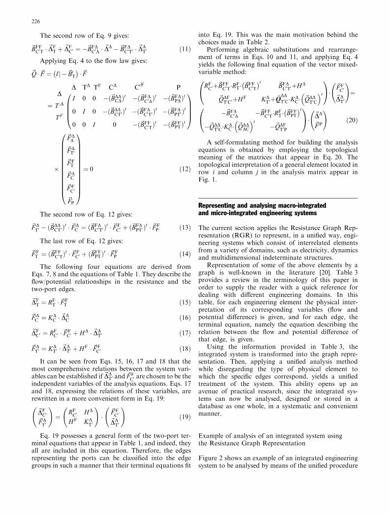
Performing algebraic substitutions and rearrange-ment of terms in Eqs. 10 and 11, and applying Eq. 4yields the following final equation of the vector mixed-variable method:

RFC0þ~BFF

C0T�RF

T� ~BFFC0T

� �t ~BFDC0T0þHD

~QDFT0C0þHF KD

T0þ ~QDDT0C�KD

C � ~QDDT0C

� �t

0

@

1

A�~F FC0

~DDT0

!

¼

�~BFDC0D �~BFF

C0T�RF

T� ~BFFPT

� �t

�~QDDT0C�KD

C � ~QDDDC

� �t�~QDF

T0P

0

@

1

A�~DD

~F P

!

ð20Þ

A self-formulating method for building the analysisequations is obtained by employing the topologicalmeaning of the matrices that appear in Eq. 20. Thetopological interpretation of a general element located inrow i and column j in the analysis matrix appear inFig. 1.

Representing and analysing macro-integratedand micro-integrated engineering systems

The current section applies the Resistance Graph Rep-resentation (RGR) to represent, in a unified way, engi-neering systems which consist of interrelated elementsfrom a variety of domains, such as electricity, dynamicsand multidimensional indeterminate structures.

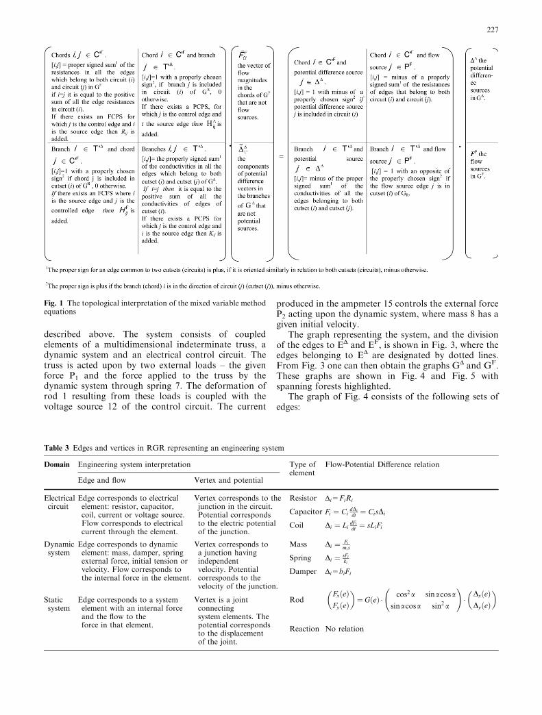
Representation of some of the above elements by agraph is well-known in the literature [20]. Table 3provides a review in the terminology of this paper inorder to supply the reader with a quick reference fordealing with different engineering domains. In thistable, for each engineering element the physical inter-pretation of its corresponding variables (flow andpotential difference) is given, and for each edge, theterminal equation, namely the equation describing therelation between the flow and potential difference ofthat edge, is given.

Using the information provided in Table 3, theintegrated system is transformed into the graph repre-sentation. Then, applying a unified analysis methodwhile disregarding the type of physical element towhich the specific edges correspond, yields a unifiedtreatment of the system. This ability opens up anavenue of practical research, since the integrated sys-tems can now be analysed, designed or stored in adatabase as one whole, in a systematic and convenientmanner.

Example of analysis of an integrated system usingthe Resistance Graph Representation

Figure 2 shows an example of an integrated engineeringsystem to be analysed by means of the unified procedure

226

described above. The system consists of coupledelements of a multidimensional indeterminate truss, adynamic system and an electrical control circuit. Thetruss is acted upon by two external loads – the givenforce P1 and the force applied to the truss by thedynamic system through spring 7. The deformation ofrod 1 resulting from these loads is coupled with thevoltage source 12 of the control circuit. The current

produced in the ampmeter 15 controls the external forceP2 acting upon the dynamic system, where mass 8 has agiven initial velocity.

The graph representing the system, and the divisionof the edges to ED and EF, is shown in Fig. 3, where theedges belonging to ED are designated by dotted lines.From Fig. 3 one can then obtain the graphs GD and GF.These graphs are shown in Fig. 4 and Fig. 5 withspanning forests highlighted.

The graph of Fig. 4 consists of the following sets ofedges:

Table 3 Edges and vertices in RGR representing an engineering system

Domain Engineering system interpretation Type ofelement

Flow-Potential Difference relation

Edge and flow Vertex and potential

Electricalcircuit

Edge corresponds to electricalelement: resistor, capacitor,coil, current or voltage source.Flow corresponds to electricalcurrent through the element.

Vertex corresponds to thejunction in the circuit.Potential correspondsto the electric potentialof the junction.

Resistor Di=FiRi

Capacitor Fi ¼ CidDidt ¼ CisDi

Coil Di ¼ LidFidt ¼ sLiFi

Dynamicsystem

Edge corresponds to dynamicelement: mass, damper, springexternal force, initial tension orvelocity. Flow corresponds tothe internal force in the element.

Vertex corresponds toa junction havingindependentvelocity. Potentialcorresponds to thevelocity of the junction.

Mass Di ¼ Fimis

Spring Di ¼ sFiki

Damper Di=biFi

Staticsystem

Edge corresponds to a systemelement with an internal forceand the flow to theforce in that element.

Vertex is a jointconnectingsystem elements. Thepotential correspondsto the displacementof the joint.

RodFxðeÞFyðeÞ

� �

¼GðeÞ � cos2 a sinacosa

sinacosa sin2 a

!

�DxðeÞDyðeÞ

� �

Reaction No relation

Fig. 1 The topological interpretation of the mixed variable methodequations

227

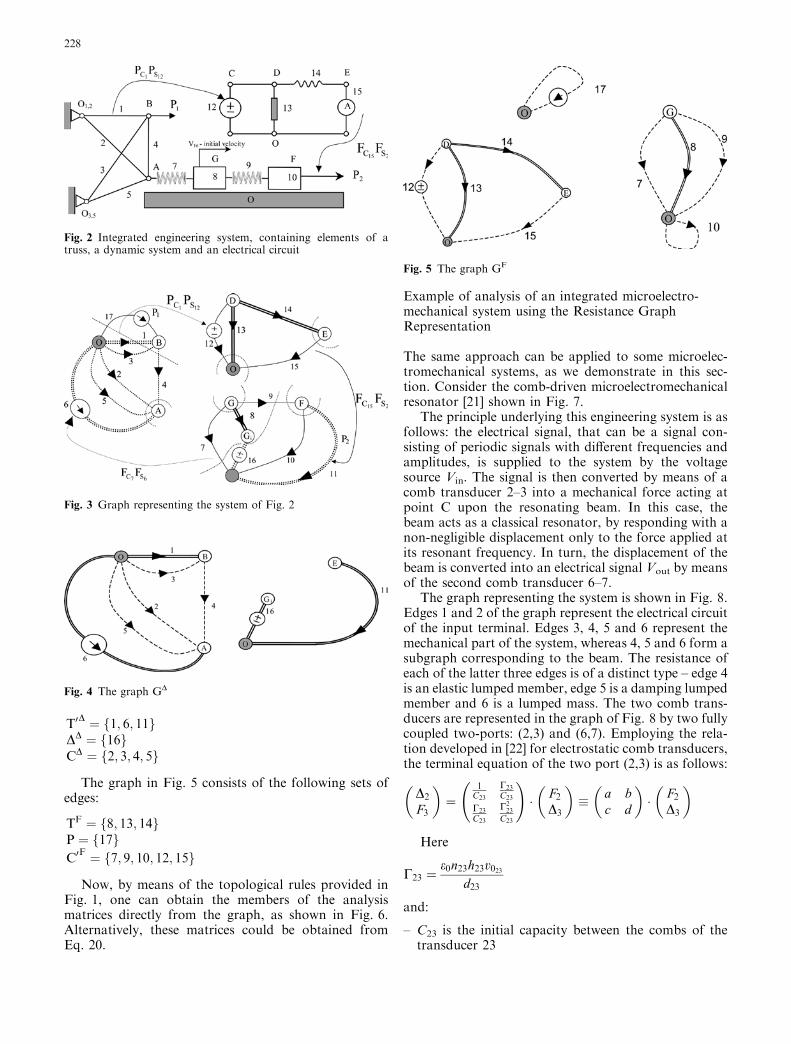
T0D ¼ f1; 6; 11g

DD ¼ f16gCD ¼ f2; 3; 4; 5g

The graph in Fig. 5 consists of the following sets ofedges:

TF ¼ f8; 13; 14gP ¼ f17gC0

F ¼ f7; 9; 10; 12; 15g

Now, by means of the topological rules provided inFig. 1, one can obtain the members of the analysismatrices directly from the graph, as shown in Fig. 6.Alternatively, these matrices could be obtained fromEq. 20.

Example of analysis of an integrated microelectro-mechanical system using the Resistance GraphRepresentation

The same approach can be applied to some microelec-tromechanical systems, as we demonstrate in this sec-tion. Consider the comb-driven microelectromechanicalresonator [21] shown in Fig. 7.

The principle underlying this engineering system is asfollows: the electrical signal, that can be a signal con-sisting of periodic signals with different frequencies andamplitudes, is supplied to the system by the voltagesource Vin. The signal is then converted by means of acomb transducer 2–3 into a mechanical force acting atpoint C upon the resonating beam. In this case, thebeam acts as a classical resonator, by responding with anon-negligible displacement only to the force applied atits resonant frequency. In turn, the displacement of thebeam is converted into an electrical signal Vout by meansof the second comb transducer 6–7.

The graph representing the system is shown in Fig. 8.Edges 1 and 2 of the graph represent the electrical circuitof the input terminal. Edges 3, 4, 5 and 6 represent themechanical part of the system, whereas 4, 5 and 6 form asubgraph corresponding to the beam. The resistance ofeach of the latter three edges is of a distinct type – edge 4is an elastic lumped member, edge 5 is a damping lumpedmember and 6 is a lumped mass. The two comb trans-ducers are represented in the graph of Fig. 8 by two fullycoupled two-ports: (2,3) and (6,7). Employing the rela-tion developed in [22] for electrostatic comb transducers,the terminal equation of the two port (2,3) is as follows:

D2

F3

� �

¼1

C23

C23

C23

C23

C23

C223

C23

!

� F2

D3

� �

� a bc d

� �

� F2

D3

� �

Here

C23 ¼e0n23h23v023

d23

and:

– C23 is the initial capacity between the combs of thetransducer 23

Fig. 3 Graph representing the system of Fig. 2

Fig. 4 The graph GD

Fig. 5 The graph GF

Fig. 2 Integrated engineering system, containing elements of atruss, a dynamic system and an electrical circuit

228

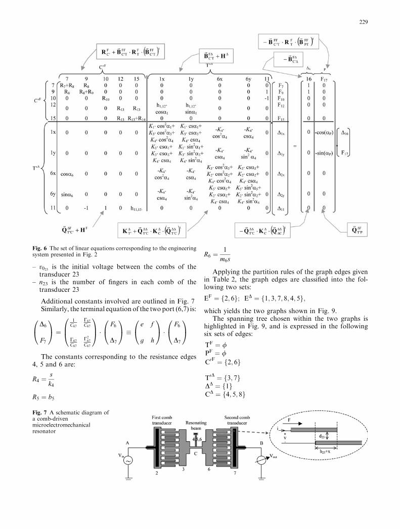
– v023 is the initial voltage between the combs of thetransducer 23

– n23 is the number of fingers in each comb of thetransducer 23

Additional constants involved are outlined in Fig. 7Similarly, the terminal equation of the two port (6,7) is:

D6

F7

0

@

1

A ¼

1C67

C67

C67

C67

C67

C267

C67

0

B@

1

CA �

F6

D7

0

@

1

A �e f

g h

0

@

1

A �F6

D7

0

@

1

A

The constants corresponding to the resistance edges4, 5 and 6 are:

R4 ¼sk4

R5 ¼ b5

R6 ¼1

m6s

Applying the partition rules of the graph edges givenin Table 2, the graph edges are classified into the fol-lowing two sets:

EF ¼ 2; 6f g; ED ¼ 1; 3; 7; 8; 4; 5f g;

which yields the two graphs shown in Fig. 9.The spanning tree chosen within the two graphs is

highlighted in Fig. 9, and is expressed in the followingsix sets of edges:

TF ¼ /PF ¼ /C0

F ¼ f2; 6g

T0D ¼ f3; 7g

DD ¼ f1gCD ¼ f4; 5; 8g

Fig. 7 A schematic diagram ofa comb-drivenmicroelectromechanicalresonator

Fig. 6 The set of linear equations corresponding to the engineeringsystem presented in Fig. 2

229

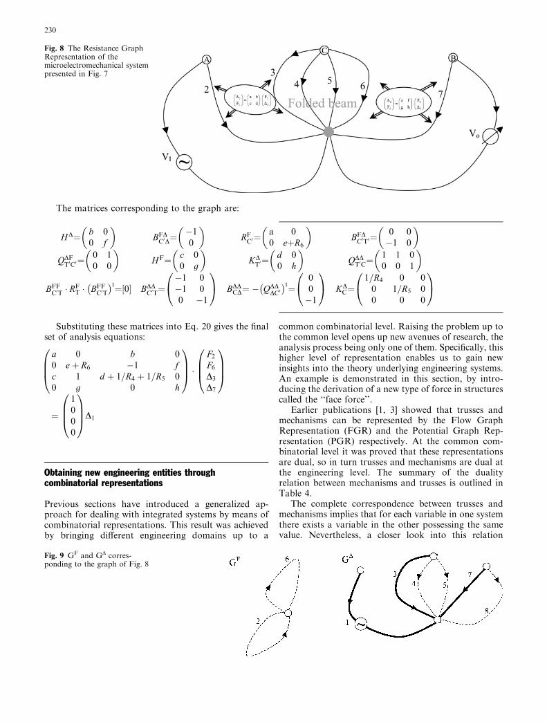
The matrices corresponding to the graph are:

Substituting these matrices into Eq. 20 gives the finalset of analysis equations:

a 0 b 00 eþ R6 �1 fc 1 d þ 1=R4 þ 1=R5 00 g 0 h

0

BB@

1

CCA�

F2

F6

D3

D7

0

BB@

1

CCA

¼

1000

0

BB@

1

CCA

D1

Obtaining new engineering entities throughcombinatorial representations

Previous sections have introduced a generalized ap-proach for dealing with integrated systems by means ofcombinatorial representations. This result was achievedby bringing different engineering domains up to a

common combinatorial level. Raising the problem up tothe common level opens up new avenues of research, theanalysis process being only one of them. Specifically, thishigher level of representation enables us to gain newinsights into the theory underlying engineering systems.An example is demonstrated in this section, by intro-ducing the derivation of a new type of force in structurescalled the ‘‘face force’’.

Earlier publications [1, 3] showed that trusses andmechanisms can be represented by the Flow GraphRepresentation (FGR) and the Potential Graph Rep-resentation (PGR) respectively. At the common com-binatorial level it was proved that these representationsare dual, so in turn trusses and mechanisms are dual atthe engineering level. The summary of the dualityrelation between mechanisms and trusses is outlined inTable 4.

The complete correspondence between trusses andmechanisms implies that for each variable in one systemthere exists a variable in the other possessing the samevalue. Nevertheless, a closer look into this relation

Fig. 9 GF and GD corres-ponding to the graph of Fig. 8

Fig. 8 The Resistance GraphRepresentation of themicroelectromechanical systempresented in Fig. 7

HD¼ b 00 f

� �

BFDC0D¼

�10

� �

RFC0¼ a 0

0 eþR6

� �

BFDC0T0¼ 0 0�1 0

� �

QDFT0C0¼ 0 1

0 0

� �

HF¼ c 00 g

� �

KDT0¼

d 00 h

� �

QDDT0C¼

1 1 00 0 1

� �

BFFC0T� RF

T � BFFC0T

� �t¼ 0½ � BDDC0T¼�1 0�1 00 �1

0

@

1

A BDDCD¼ � QDD

DC0� �t¼

00�1

0

@

1

A KDC¼

1=R4 0 00 1=R5 00 0 0

0

@

1

A

230

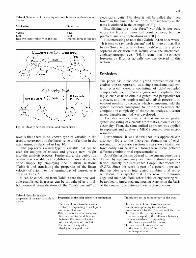
reveals that there is no known type of variable in thetruss to correspond to the linear velocity of a joint in themechanism, as depicted in Fig. 10.

This gap reveals a new type of variable that can beused for analysis of trusses and gives a new insightinto the analysis process. Furthermore, the derivationof this new variable is straightforward, since it can bedone simply by employing the dualism relations(Table 4) and translating the properties of the linearvelocity of a joint to the terminology of trusses, as isdone in Table 5.

It can be concluded from Table 5 that the new vari-able established in trusses can be thought of as a mul-tidimensional generalization of the ‘‘mesh current’’ in

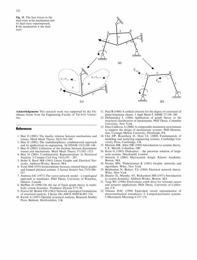
electrical circuits [19]. Here it will be called the ‘‘faceforce’’ in the truss. The action of the face forces in thetruss is outlined in the example of Fig. 11.

Establishing the ‘‘face force’’ variable is not onlyimportant from a theoretical point of view, but haspractical analysis applications as well [3].

It is interesting to note that Gabriel Kron once wrote:‘‘It is easy to say �mesh current� and let it go at that. Butto say �force acting in a closed mesh� requires a philo-sophical dissertation that would leave the mechanicalengineer unresponsive.’’ [16]. It seems that the conceptforeseen by Kron is actually the one derived in thissection.

Conclusions

The paper has introduced a graph representation thatenables one to represent, as a single mathematical sys-tem, physical systems consisting of tightly-coupledcomponents from different engineering disciplines. Do-ing so enables us to obtain a generalized perspective fora system, and then apply a unified analysis process to it,without needing to consider which engineering field thesystem elements correspond to. In order to reduce thecomputation complexity of the system analysis, a vectormixed variable method was developed.

The idea was demonstrated first on an integratedsystem consisting of elements from statics, dynamics andelectricity. Then, the same unified approach was appliedto represent and analyse a MEMS comb-driven micro-resonator.

Furthermore, it was shown that this approach canalso contribute to the theoretical foundation of engi-neering. In the previous section it was shown that a newforce entity can be derived from the relations betweendifferent combinatorial representations.

All of the results introduced in the current paper werederived by applying only one combinatorial represen-tation, namely the Resistance Graph Representation(RGR). Since this work is part of a general approachthat includes several interrelated combinatorial repre-sentations, it is expected that in the near future knowl-edge and methods from other fields of engineering willbe applied to integrated engineering systems on the basisof the connections between these representations.

Table 4 Summary of the duality relations between mechanisms andtrusses

Mechanism Dual truss

Vertex FaceLink RodRelative linear velocity of the link Internal force in the rod

Fig. 10 Duality between trusses and mechanisms

Table 5 Establishing theproperties of the new variable intrusses

Properties of the joint velocity in mechanism Translation to the terminology of the truss

The variable is a two-dimensionalvector corresponding to each jointin the mechanism

The new variable is a two-dimensionalvector corresponding to each face(area bounded by the truss rods) of the truss

Relative velocity of a mechanismlink is equal to the differencebetween the linear velocitiesof the end joints of this link

The force in the correspondingtruss rod is equal to the difference betweenthe new variables correspondingto the faces separated by this rod

The linear velocity of afixed joint is equal to zero

The new variable correspondingto the external face of thetruss is equal to zero

231

Acknowledgements This research work was supported by the Fle-ishman Grant from the Engineering Faculty of Tel-Aviv Univer-sity.

References

1. Shai O (2001) The duality relation between mechanisms andtrusses. Mech Mach Theory 36(3):343–369

2. Shai O (2001) The multidisciplinary combinatorial approachand its applications in engineering. AI EDAM 15(2):109–144

3. Shai O (2002) Utilization of the dualism between determinatetrusses and mechanisms. Mech Mach Theory 37:1307–1323

4. Shai O (2001) Combinatorial Representations in StructuralAnalysis. J Comput Civil Eng 15(3):193 – 207

5. Seshu S, Reed MB (1961) Linear Graphs and Electrical Net-works. Addison-Wesley, Boston, MA

6. Trent HM (1955) Isomorphisms between oriented linear graphsand lumped physical systems. J Acoust Society Am 27(3):500–527

7. Andrews GC (1971) The vector-network model – a topologicalapproach to mechanics. PhD Thesis, University of Waterloo,Ontario, Canada

8. McPhee JJ (1996) On the use of linear graph theory in multi-body system dynamics. Nonlinear Dynam 9:73–90

9. Fenves SJ, Branin FH (1963) Network topological formulationof structural analysis. J Struct Div-ASCE 89(ST4):483–514

10. Kaveh A (1997) Optimal structural analysis. Research StudiesPress, Baldock, Hertfordshire, UK

11. Paul B (1960) A unified criterion for the degree of constraint ofplane kinematic chains. J Appl Mech-T ASME 27:196–200

12. Dobrjanskyj L (1966) Application of graph theory to thestructural classification of mechanisms. PhD Thesis, ColumbiaUniversity, New York

13. Diaz-Calderon A (2000) A composable simulation environmentto support the design of mechatronic systems. PhD Disserta-tion, Carnegie Mellon University, Pittsburgh, PA

14. Cha DP, Rosenberg JJ, Dym CL (2000) Fundamentals ofmodeling and analyzing engineering systems. Cambridge Uni-versity Press, Cambridge, UK

15. Martens HR, Allen DR (1969) Introduction to systems theory.C.E. Merrill, Columbus, OH

16. Kron G (1963) Diakoptics – the piecewise solution of large-scale systems. Macdonald, London

17. Senturia S (2001) Microsystem design. Kluwer Academic,Boston, MA

18. Swamy MN, Thulasiraman K (1981) Graphs: networks andalgorithms. Wiley, New York

19. Balabanian N, Bickart TA (1969) Electrical network theory.Wiley, New York

20. Shearer JL, Murphy AT, Richardson HH (1971) Introductionto system dynamics. Addison-Wesley, Boston, MA

21. Tang WC (1990) Electrostatic comb drive for resonant sensorand actuator applications. PhD Thesis, University of Califor-nia, CA

22. Tilmans HAC (1996) Equivalent circuit representation ofelectromechanical transducers: I. Lumped-parameter systems.J Micromech Microeng 6:157–176

Fig. 11 The face forces in thedual truss: a the mechanism andits dual truss superimposed;b the mechanism; c the dualtruss

232