Introduction to Introduction to Transmission Market Design in the US: Transmission Market Design in the US:

LocationalLocational Marginal PricingMarginal PricingNGInfraNGInfra AcademyAcademy

Electricity & COElectricity & CO22 Markets TrackMarkets Track

Benjamin F. Hobbs, Ph.D.Benjamin F. Hobbs, Ph.D.

bhobbs@jhu.edubhobbs@jhu.eduDepartment of Geography & Environmental EngineeringDepartment of Geography & Environmental Engineering

Whiting School of Engineering, The Johns Hopkins UniversityWhiting School of Engineering, The Johns Hopkins University

California ISO Market Surveillance CommitteeCalifornia ISO Market Surveillance Committee

Electricity Policy Research Group, University of CambridgeElectricity Policy Research Group, University of CambridgeThanks to Udi Helman, Richard OThanks to Udi Helman, Richard O’’Neill , Michael Rothkopf, Neill , Michael Rothkopf, William Stewart, Jim Bushnell, Frank Wolak, Anjali Sheffrin, William Stewart, Jim Bushnell, Frank Wolak, Anjali Sheffrin, Keith Casey, Shmuel Oren, Bill Hogan for discussions & ideasKeith Casey, Shmuel Oren, Bill Hogan for discussions & ideas

JHU___

22

JHU___

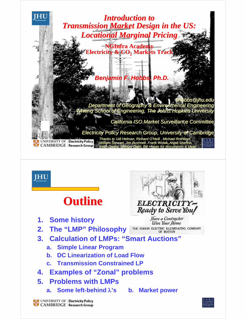
OutlineOutline

1. Some history2. The “LMP” Philosophy3. Calculation of LMPs: “Smart Auctions”

a. Simple Linear Program b. DC Linearization of Load Flowc. Transmission Constrained LP

4. Examples of “Zonal” problems5. Problems with LMPs

a. Some left-behind λ’s b. Market power

33

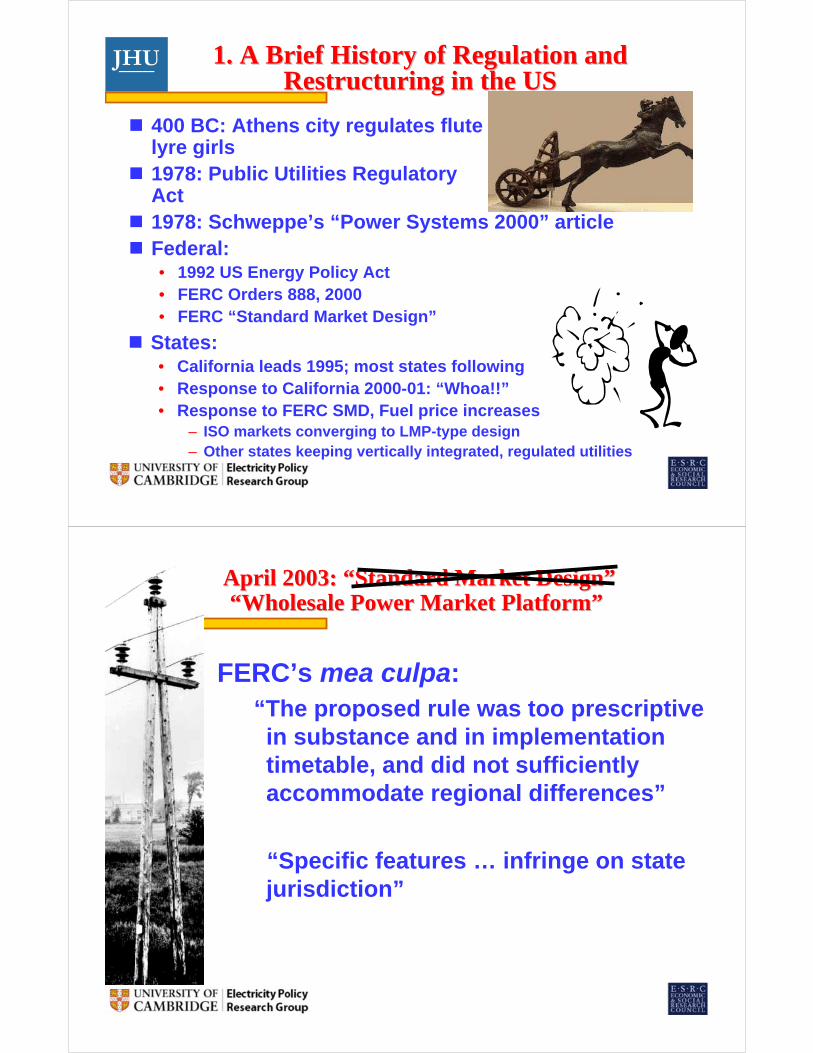
JHU___ 1. A Brief History of Regulation and 1. A Brief History of Regulation and Restructuring in the USRestructuring in the US

400 BC: Athens city regulates flute & lyre girls1978: Public Utilities Regulatory Policy Act1978: Schweppe’s “Power Systems 2000” articleFederal: • 1992 US Energy Policy Act• FERC Orders 888, 2000• FERC “Standard Market Design”

States: • California leads 1995; most states following• Response to California 2000-01: “Whoa!!”• Response to FERC SMD, Fuel price increases

– ISO markets converging to LMP-type design– Other states keeping vertically integrated, regulated utilities

44

JHU___ April 2003: “Standard Market Design” April 2003: “Standard Market Design”

FERC’s mea culpa:“The proposed rule was too prescriptive in substance and in implementation timetable, and did not sufficiently accommodate regional differences”

“Specific features … infringe on state jurisdiction”

“Wholesale Power Market Platform”“Wholesale Power Market Platform”

55

JHU___ Market Design Principles of “Platform”Market Design Principles of “Platform”

Grid operation:• Regional

• Independent

• Congestion pricing (LMP)

Grid planning:• Regional

• State and stakeholder led

Resource (= gen capacity) adequacy• State led

66

JHU___ More Principles of “Platform”More Principles of “Platform”

Spot markets:• Day ahead and balancing• Integrated energy, ancillary services, transmission• “Smart Auctions”

– Auctions solved by optimization models

Firm transmission rights• Financial, not physical• Don’t need to auction

– Allocation can protect participants from harm

Market power• Market-wide and local mitigation• Monitoring

77

JHU___

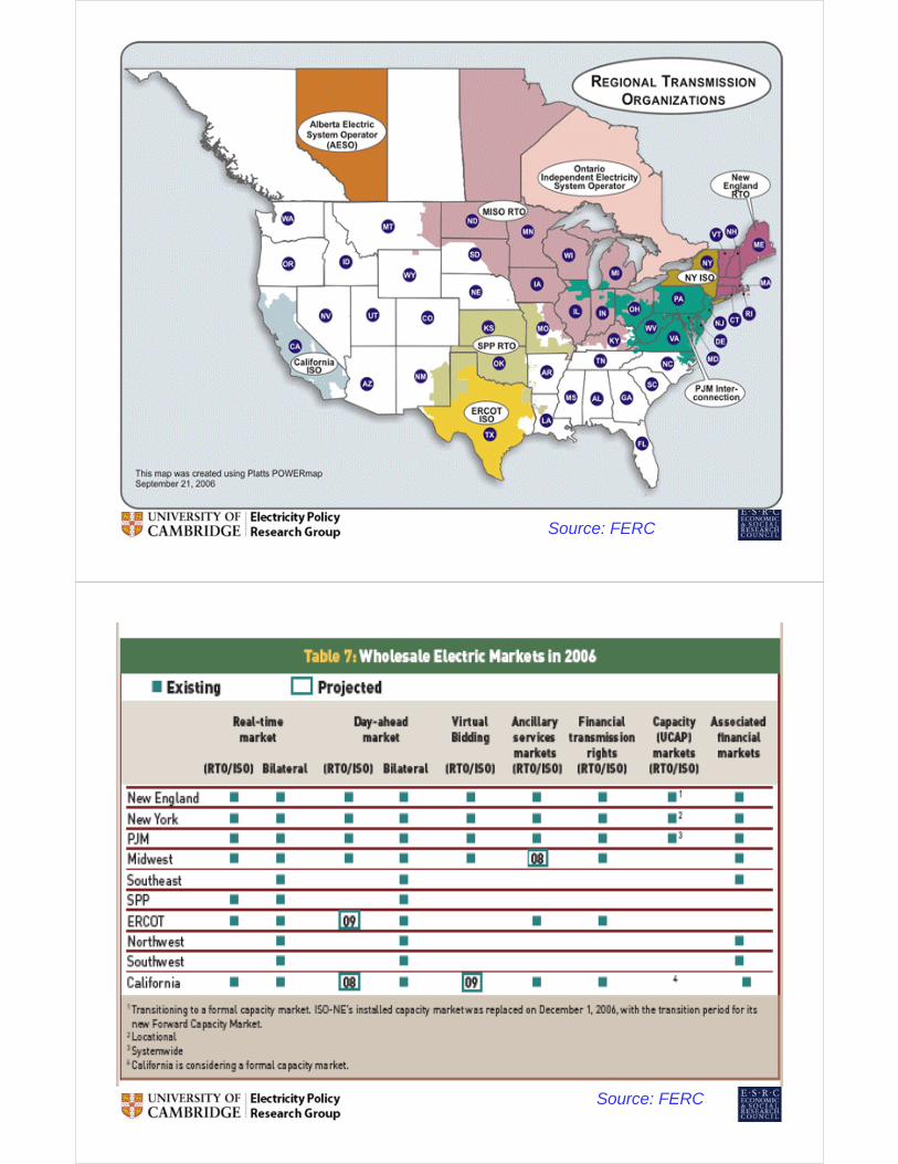
Source: FERC

88

JHU___

Source: FERC

99

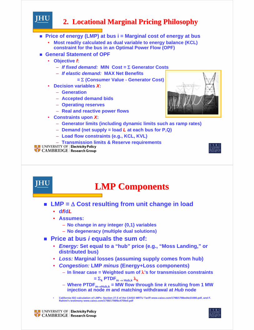
JHU___ 2. 2. LocationalLocational Marginal Pricing PhilosophyMarginal Pricing Philosophy

Price of energy (LMP) at bus i = Marginal cost of energy at bus• Most readily calculated as dual variable to energy balance (KCL)

constraint for the bus in an Optimal Power Flow (OPF)

General Statement of OPF• Objective f:

– If fixed demand: MIN Cost = Σ Generator Costs– If elastic demand: MAX Net Benefits

= Σ (Consumer Value - Generator Cost)• Decision variables X:

– Generation – Accepted demand bids– Operating reserves– Real and reactive power flows

• Constraints upon X:– Generator limits (including dynamic limits such as ramp rates)– Demand (net supply = load L at each bus for P,Q)– Load flow constraints (e.g., KCL, KVL)– Transmission limits & Reserve requirements

1010

JHU___ LMP ComponentsLMP Components

LMP = Δ Cost resulting from unit change in load• df/dL• Assumes:

– No change in any integer {0,1} variables– No degeneracy (multiple dual solutions)

Price at bus i equals the sum of:• Energy: Set equal to a “hub” price (e.g., “Moss Landing,” or

distributed bus)• Loss: Marginal losses (assuming supply comes from hub)• Congestion: LMP minus (Energy+Loss components)

– In linear case = Weighted sum of λ’s for transmission constraints= Σk PTDFm → Hub,k λk

– Where PTDFm→Hub,k = MW flow through line k resulting from 1 MW injection at node m and matching withdrawal at Hub node

• California ISO calculation of LMPs: Section 27.5 of the CAISO MRTU Tariff www.caiso.com/1798/1798ed4e31090.pdf, and F. Rahimi's testimony www.caiso.com/1798/1798f6c4709e0.pdf

1111

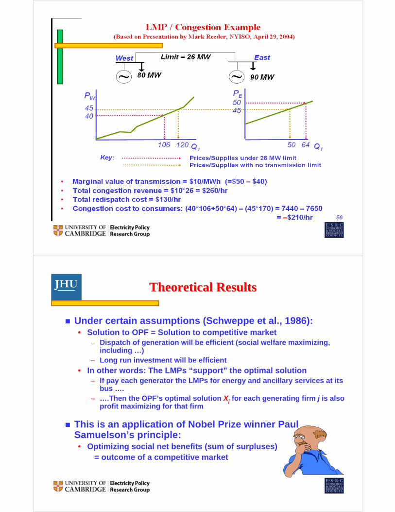
JHU___ LMP / Congestion ExampleLMP / Congestion Example(Based on Presentation by Mark Reeder, NYISO, April 29, 2004)(Based on Presentation by Mark Reeder, NYISO, April 29, 2004)

• Marginal value of transmission = ?• Total congestion revenue = ?• Total redispatch cost = ?

~WestWest EastEast

~Limit = 26 MW

80 MW 90 MW

PPWW

QQ11106 120106 120

45454040

QQ1150 6450 64

50504545

PPEE

Key:Key:Prices/Supplies with no transmission limitPrices/Supplies under 26 MW limit

1212

JHU___ Theoretical ResultsTheoretical Results

Under certain assumptions (Schweppe et al., 1986):• Solution to OPF = Solution to competitive market

– Dispatch of generation will be efficient (social welfare maximizing, including …)

– Long run investment will be efficient

• In other words: The LMPs “support” the optimal solution– If pay each generator the LMPs for energy and ancillary services at its

bus ….– ….Then the OPF’s optimal solution Xj for each generating firm j is also

profit maximizing for that firm

This is an application of Nobel Prize winner Paul Samuelson’s principle:• Optimizing social net benefits (sum of surpluses)

= outcome of a competitive market

1313

JHU___ AssumptionsAssumptions

No market power

No price caps, etc.

Perfect information

Costs are convex

• No unit commitment constraints

• No lumpy investments or scale

economies

Constraints define convex set

• E.g., AC load flow non convex

Can compute the solution

• ~104 buses, 103 generators

1414

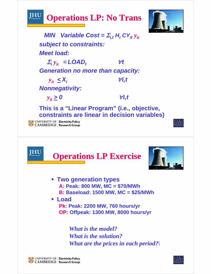
JHU___ 3. Computing 3. Computing LMPsLMPsa. a. System Dispatch “Linear Program” sans TransmissionSystem Dispatch “Linear Program” sans Transmission

Basic model • Cost minimization, pure thermal system, deterministic

In words:• Choose level of operation of each generator (decision variable),• …to minimize total system cost (objective)• …subject to load, capacity limit (constraints)

Decision variable:yit = megawatt [MW] output of generating unit i (i=1,..,I)

during period t (t=1,..,T)Coefficients:CYit = variable operating cost [$/MWh] for yit

Xi = MW capacity of generating unit i. LOADt = MW demand to be met in period tHt = length of period t [hours/yr]. (Note: in pure thermal

system, periods do not need to be sequential)

1515

JHU___ Operations LP: No TransOperations LP: No Trans

MIN Variable Cost = Σi,t Ht CYit yit

subject to constraints:

Meet load:

Σi yit = LOADt ∀t

Generation no more than capacity:

yit < Xi ∀i,t

Nonnegativity:

yit > 0 ∀i,t

This is a “Linear Program” (i.e., objective, constraints are linear in decision variables)

1616

JHU___ Operations LP ExerciseOperations LP Exercise

Two generation typesA: Peak: 800 MW, MC = $70/MWhB: Baseload: 1500 MW, MC = $25/MWh

LoadPk: Peak: 2200 MW, 760 hours/yrOP: Offpeak: 1300 MW, 8000 hours/yr

What is the model?What is the solution?What are the prices in each period?\

1717

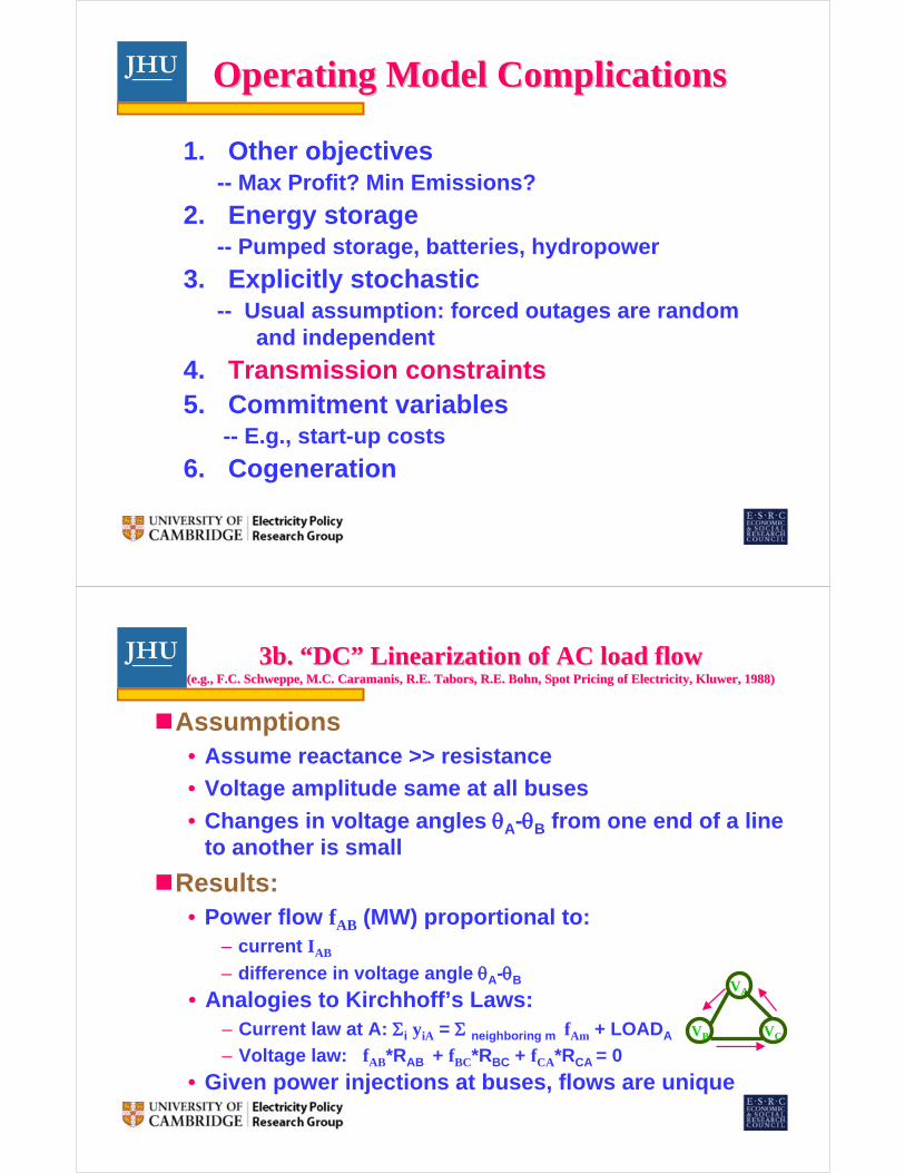
JHU___ Operating Model ComplicationsOperating Model Complications

1. Other objectives -- Max Profit? Min Emissions?

2. Energy storage -- Pumped storage, batteries, hydropower

3. Explicitly stochastic -- Usual assumption: forced outages are random

and independent

4. Transmission constraints5. Commitment variables

-- E.g., start-up costs

6. Cogeneration

1818

JHU___ 3b. “DC” Linearization of AC load flow3b. “DC” Linearization of AC load flow(e.g., (e.g., F.C. F.C. SchweppeSchweppe, M.C. , M.C. CaramanisCaramanis, R.E. Tabors, , R.E. Tabors, RR.E. Bohn, Spot Pricing of Electricity, .E. Bohn, Spot Pricing of Electricity, KluwerKluwer, , 1988)1988)

Assumptions• Assume reactance >> resistance

• Voltage amplitude same at all buses

• Changes in voltage angles θA-θB from one end of a line to another is small

Results:• Power flow fAB (MW) proportional to:

– current IAB

– difference in voltage angle θA-θB VA

VB VC

• Analogies to Kirchhoff’s Laws:– Current law at A: Σi yiA = Σ neighboring m fAm + LOADA

– Voltage law: fAB*RAB + fBC*RBC + fCA*RCA = 0

• Given power injections at buses, flows are unique

1919

JHU___ Example of “DC” Load FlowExample of “DC” Load Flow

A

B C

All lines have reactance = 1

~ A

B C

~100 MW

100 MW

67 MW

33 MW

33 MW

Kirchhoff’s Current Law at C:+33 + 67 - 100 = 0

Kirchhoff’s Voltage Law:1*33 + 1*33 + 1*(-67) = 0

A

B C

~300 MW

300 MW

200 MW

100 MW

100 MW

Proportionality!

2020

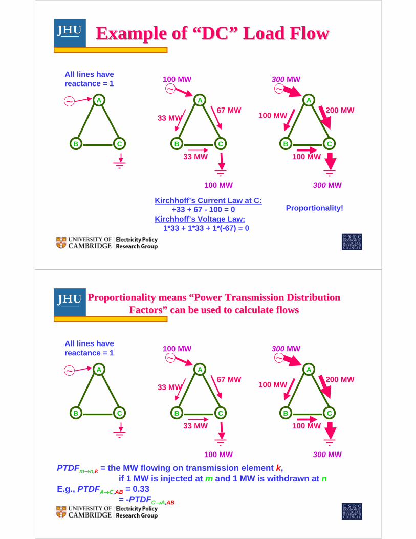
JHU___ Proportionality means “Power Transmission Distribution Proportionality means “Power Transmission Distribution FactorsFactors” can be used to calculate flows” can be used to calculate flows

A

B C

All lines have reactance = 1

~ A

B C

~100 MW

100 MW

67 MW

33 MW

33 MW

A

B C

~300 MW

300 MW

200 MW

100 MW

100 MW

PTDFm→n,k = the MW flowing on transmission element k, if 1 MW is injected at m and 1 MW is withdrawn at n

E.g., PTDFA→C,AB = 0.33 = -PTDFC→A,AB

2121

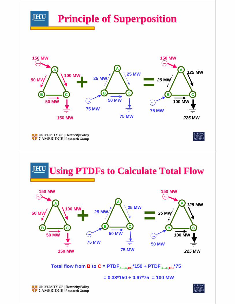
JHU___ Principle of SuperpositionPrinciple of Superposition

A

B C

~150 MW

150 MW

100 MW

50 MW

50 MW

A

B C

~75 MW

75 MW

25 MW

50 MW

25 MW+A

B C

~150 MW

225 MW

125 MW

100 MW

25 MW

~75 MW

=

2222

JHU___ Using Using PTDFsPTDFs to Calculate Total Flowto Calculate Total Flow

Total flow from B to C = PTDFA→C,BC*150 + PTDFB→C,BC*75

A

B C

~150 MW

150 MW

100 MW

50 MW

50 MW

A

B C

~75 MW

75 MW

25 MW

50 MW

25 MW

A

B C

~150 MW

225 MW

125 MW

100 MW

25 MW

~50 MW

+ =

= 0.33*150 + 0.67*75 = 100 MW

2323

JHU___

A

BC

~25 $/MWh

400 MW

~70 $/MWh

100 MW Limit

500 MW

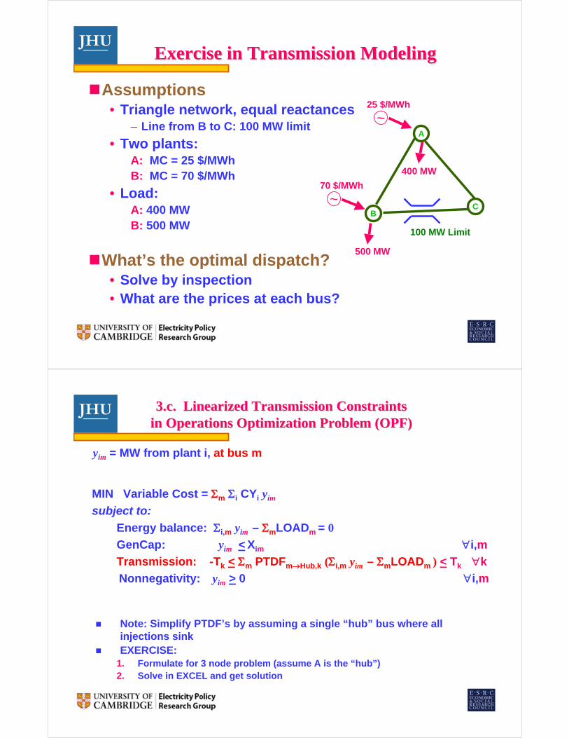
Exercise in Transmission ModelingExercise in Transmission Modeling

Assumptions• Triangle network, equal reactances

– Line from B to C: 100 MW limit

• Two plants: A: MC = 25 $/MWhB: MC = 70 $/MWh

• Load:A: 400 MWB: 500 MW

What’s the optimal dispatch?• Solve by inspection• What are the prices at each bus?

2424

JHU___ 3.c. 3.c. LinearizedLinearized Transmission Constraints Transmission Constraints in Operations Optimization Problem (OPF)in Operations Optimization Problem (OPF)

yim = MW from plant i, at bus m

Note: Simplify PTDF’s by assuming a single “hub” bus where all injections sinkEXERCISE:

1. Formulate for 3 node problem (assume A is the “hub”)2. Solve in EXCEL and get solution

MIN Variable Cost = Σm Σi CYi yim

subject to:

Energy balance: Σi,m yim – ΣmLOADm = 0

GenCap: yim < Xim ∀i,m

Transmission: -Tk < Σm PTDFm→Hub,k (Σi,m yim – ΣmLOADm ) < Tk ∀k

Nonnegativity: yim > 0 ∀i,m

2525

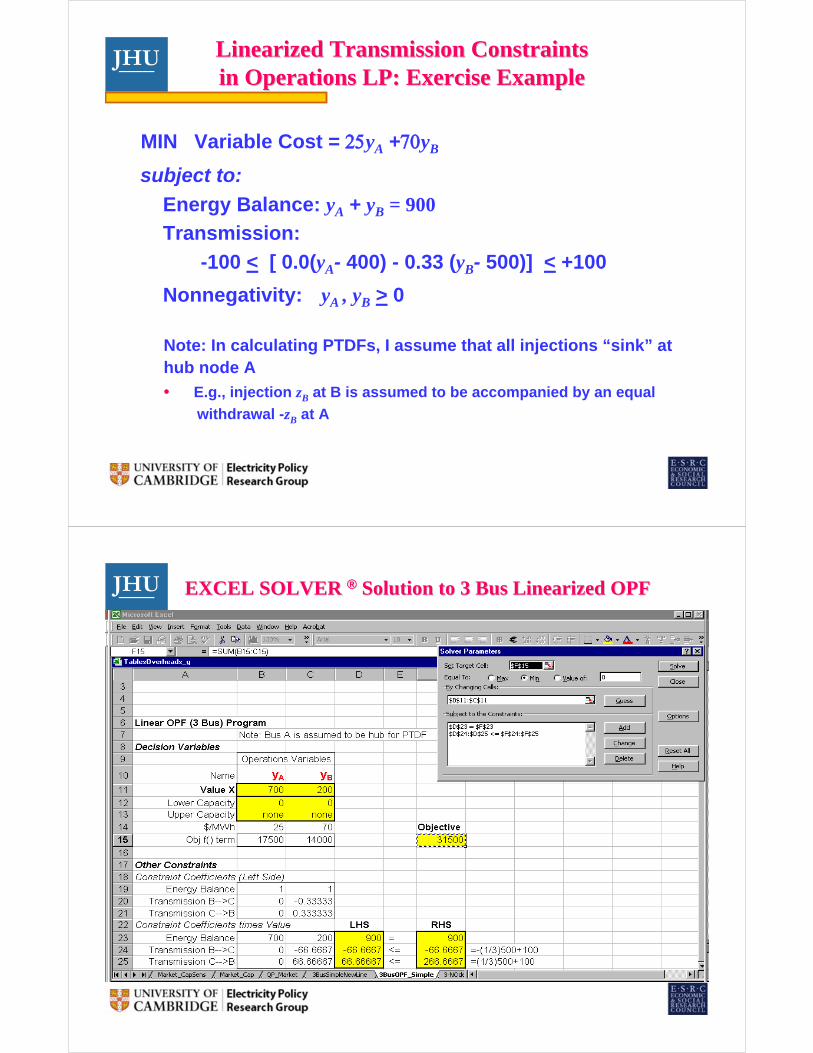
JHU___LinearizedLinearized Transmission Constraints Transmission Constraints in Operations LP: Exercise Examplein Operations LP: Exercise Example

subject to:

Energy Balance: yA + yB = 900

Transmission:

-100 < [ 0.0(yA- 400) - 0.33 (yB- 500)] < +100

Nonnegativity: yA , yB > 0

MIN Variable Cost = 25yA +70yB

Note: In calculating PTDFs, I assume that all injections “sink” at hub node A

• E.g., injection zB at B is assumed to be accompanied by an equal

withdrawal -zB at A

2626

JHU___ EXCEL SOLVER EXCEL SOLVER ®® Solution to 3 Bus Solution to 3 Bus LinearizedLinearized OPFOPF

2727

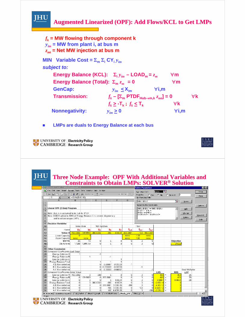
JHU___ Augmented Augmented LinearizedLinearized (OPF): Add Flows/KCL to Get (OPF): Add Flows/KCL to Get LMPsLMPs

fk = MW flowing through component kyim = MW from plant i, at bus mzmt = Net MW injection at bus m

MIN Variable Cost = Σm Σi CYi yim

subject to:

Energy Balance (KCL): Σi yim – LOADm = zm ∀m

Energy Balance (Total): Σm zm = 0 ∀m

GenCap: yim < Xim ∀i,m

Transmission: fk – [Σm PTDFHub→m,k zmt] = 0 ∀k

fk > -Tk ; fk < Tk ∀k

Nonnegativity: yim > 0 ∀i,m

LMPs are duals to Energy Balance at each bus

2828

JHU___ Three Node Example: OPF With Additional Variables and Three Node Example: OPF With Additional Variables and Constraints to Obtain Constraints to Obtain LMPsLMPs: SOLVER: SOLVER®® SolutionSolution

2929

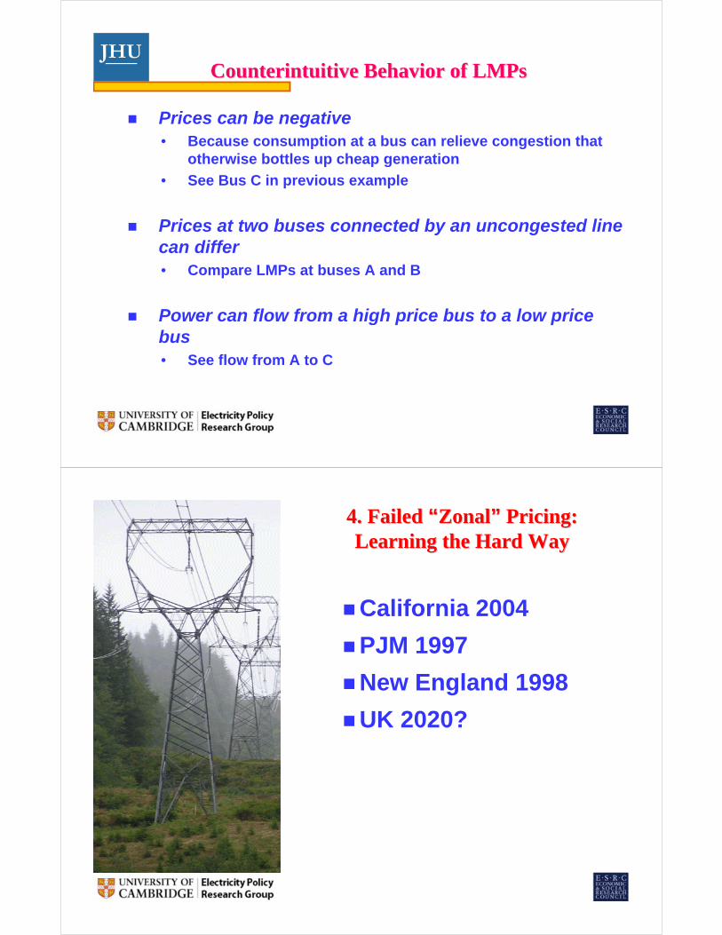
JHU___Counterintuitive Behavior of Counterintuitive Behavior of LMPsLMPs

Prices can be negative• Because consumption at a bus can relieve congestion that

otherwise bottles up cheap generation

• See Bus C in previous example

Prices at two buses connected by an uncongested line can differ• Compare LMPs at buses A and B

Power can flow from a high price bus to a low price bus• See flow from A to C

3030

JHU___ 4. Failed 4. Failed ““ZonalZonal”” Pricing:Pricing:Learning the Hard WayLearning the Hard Way

California 2004

PJM 1997

New England 1998

UK 2020?

3131

JHU___ The The ““DECDEC”” Game in Zonal MarketsGame in Zonal Markets

“System Redispatch Model”• ISO ignores congestion day ahead• ISO pays to resolve congestion in real time.

Clear zonal market day ahead (DA):• All generator bids used to create supply curve in zone• Clear supply against zonal load• All accepted bids paid DA price

In real-time, “intrazonal congestion” arises—constraint violations must be eliminated• “INC” needed generation (e.g., in load pockets) that wasn’t taken

DA– Pay them > DA price

• “DEC” unneeded generation (e.g., in gen pockets) that can’t be used– Allow generator to pay back < DA price

3232

JHU___ Problems arising from Problems arising from ““DECDEC”” GamesGames

Problem 1: Congestion worsens• The generators you want won’t enter the DA market• The generators you don’t want will• Real-time congestion worsens

Problem 2: Encourages DA bilateral contracts with “cheap” DEC’ed generation• Destroyed PJM zonal market in 1997

Problem 3: DEC game is a money machine• Gen pocket generators bid cheaply, knowing they’ll be taken

and can buy back at low price– E.g., PDA = $70/MWh, PDEC = $30– You make $40 for doing nothing

• Market power not needed for game (but can make it worse)• E.g., California 2004

3333

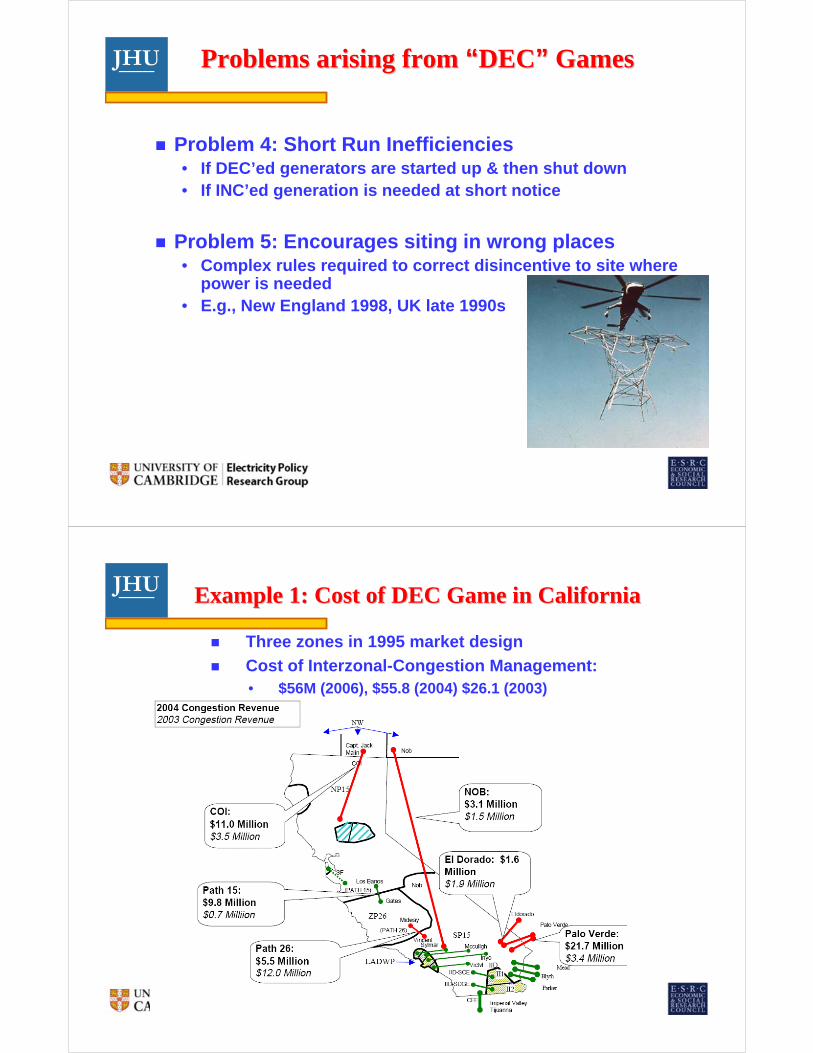
JHU___ Problems arising from Problems arising from ““DECDEC”” GamesGames

Problem 4: Short Run Inefficiencies• If DEC’ed generators are started up & then shut down• If INC’ed generation is needed at short notice

Problem 5: Encourages siting in wrong places• Complex rules required to correct disincentive to site where

power is needed• E.g., New England 1998, UK late 1990s

3434

JHU___ Example 1: Cost of DEC Game in CaliforniaExample 1: Cost of DEC Game in California

Three zones in 1995 market design

Cost of Interzonal-Congestion Management: • $56M (2006), $55.8 (2004) $26.1 (2003)

3535

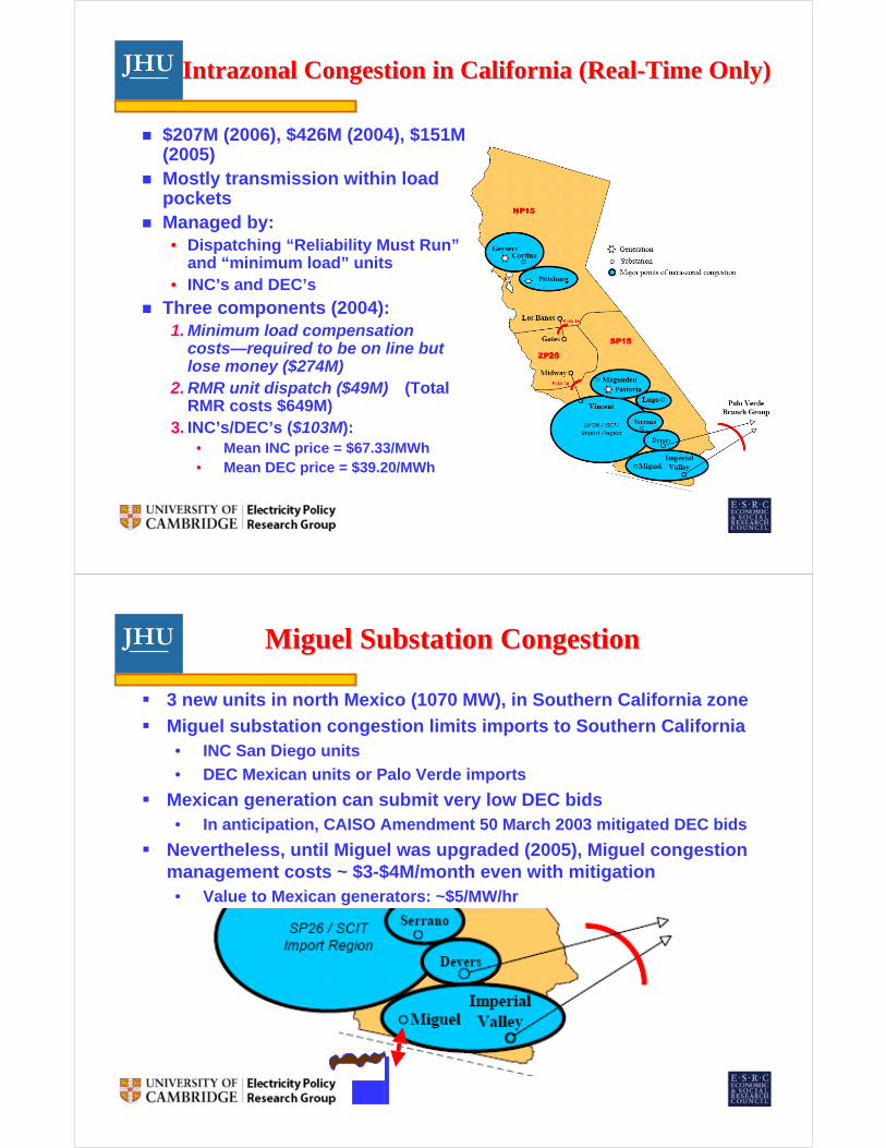
JHU___ IntrazonalIntrazonal Congestion in California (RealCongestion in California (Real--Time Only)Time Only)

$207M (2006), $426M (2004), $151M (2005)Mostly transmission within load pocketsManaged by:• Dispatching “Reliability Must Run”

and “minimum load” units• INC’s and DEC’s

Three components (2004):1. Minimum load compensation

costs—required to be on line but lose money ($274M)

2. RMR unit dispatch ($49M) (Total RMR costs $649M)

3. INC’s/DEC’s ($103M): • Mean INC price = $67.33/MWh• Mean DEC price = $39.20/MWh

3636

JHU___ Miguel Substation CongestionMiguel Substation Congestion

3 new units in north Mexico (1070 MW), in Southern California zone

Miguel substation congestion limits imports to Southern California• INC San Diego units

• DEC Mexican units or Palo Verde imports

Mexican generation can submit very low DEC bids• In anticipation, CAISO Amendment 50 March 2003 mitigated DEC bids

Nevertheless, until Miguel was upgraded (2005), Miguel congestion management costs ~ $3-$4M/month even with mitigation• Value to Mexican generators: ~$5/MW/hr

3737

JHU___ Example 2: PJM Zonal CollapseExample 2: PJM Zonal Collapse

New (1997) PJM market had zonal day-ahead market• Congestion would be cleared by “INC’s” and “DEC’s” in real-time• Congestion costs uplifted

Generators had two options: • Bid into zonal market • Bilaterals (sign contract with load,

submit fixed schedule)

Hogan’s generator intelligence test:• You have three possible sources of power

– Day ahead: zonal $30/MWh– Bilateral with west (cheap) zone: $12/MWh– Bilateral with east (costly) zone: $89/MWh

• Result: HUGE number of infeasible bilaterals with western generation• PJM emergency restrictions June 1997

PJM requested LMP and FERC approved; operational in April 1998• The important issue is not the total cost of transmission -- it’s the incentives

when congestion occurs(Source: W. Hogan, Restructuring the Electricity Market: Institutions for Network Systems, April 1999)

3838

JHU___Example 3: Example 3:

Perverse Perverse SitingSiting Incentives in New EnglandIncentives in New England

Before restructuring, New England’s power pool (NEPOOL) had a single zone and energy price• Complex planning process required transmission investment along

with generation to minimize impact of new generators on older units

In response to market opening, approximately 30 GW new plant construction was announced in late 1990s (doubling capacity)• To deal with perverse siting incentives, NEPOOL proposed complex

rules for new generators, requiring extensive studies of system impacts and expensive investments in the transmission system.

• Rules would increase costs for entry and delay it, protecting existing generators from competition

October 1998, FERC struck down rules as discriminatory and anticompetitive responses to the defective congestion management system• ISO-NE submitted a LMP proposal in 1999 which was accepted

(See W. Hogan, ibid. )

3939

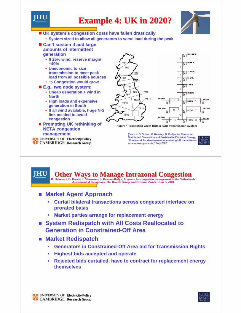
JHU___ Example 4: UK in 2020?Example 4: UK in 2020?

(Source: G. Strbac, C. Ramsay, D. Pudjianto, Centre for Distributed Generation and Sustainable Electrical Energy, “Framework for development of enduring UK transmission access arrangements,” July 2007

Can’t sustain if add large amounts of intermittent generation

• If 25% wind, reserve margin ~40%

• Uneconomic to size transmission to meet peak load from all possible sources

• ⇒ Congestion would growE.g., two node system:

• Cheap generation + wind in North

• High loads and expensive generation in South

• If all wind available, huge N-S link needed to avoid congestion

Prompting UK rethinking of NETA congestion management

UK system’s congestion costs have fallen drastically• System sized to allow all generators to serve load during the peak

4040

JHU___ Other Ways to Manage Other Ways to Manage IntrazonalIntrazonal CongestionCongestionR. R. HakvoortHakvoort, D. Harris, J. , D. Harris, J. MeeuwsenMeeuwsen, S. , S. HesmondhalghHesmondhalgh, A system for congestion management in the Netherlands, A system for congestion management in the Netherlands

Assessment of the options, The Brattle Group and Assessment of the options, The Brattle Group and DCisionDCision, Zwolle, June 5, 2009, Zwolle, June 5, 2009

Market Agent Approach• Curtail bilateral transactions across congested interface on

prorated basis

• Market parties arrange for replacement energy

System Redispatch with All Costs Reallocated to Generation in Constrained-Off Area

Market Redispatch• Generators in Constrained-Off Area bid for Transmission Rights

• Highest bids accepted and operate

• Rejected bids curtailed, have to contract for replacement energythemselves

4141

JHU___ 5. Remaining Problems of LMP:5. Remaining Problems of LMP:a. Lefta. Left--behind behind λλ’’s s

Ideally, LMPs should reflect all constraints

Spatial λ’s left behind:• “The seams issue” – interconnected systems with different

congestion management systems– Can lead to “Death Star”-type games (“money machines”)

Temporal λ’s left behind:• Ramp rates not considered in real-time LMPs

– Distorts incentives for investment in flexible generation

Interacting commodity (ancillary services) λ’s left behind:• Operator constraints not priced

– Can systematically depress energy prices

The problem of nonconvex costs• Unit commitment (min run, start up costs)

– Marginal costs ambiguous

4242

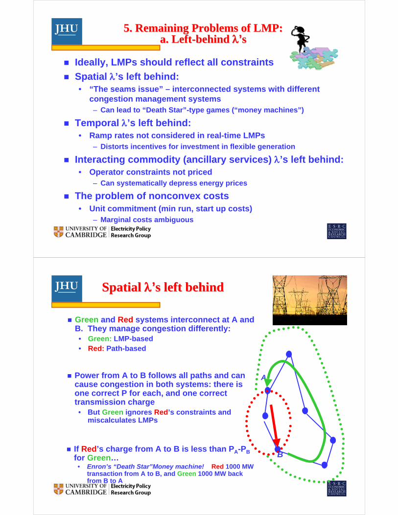
JHU___ Spatial Spatial λλ’’s left behinds left behind

Green and Red systems interconnect at A and B. They manage congestion differently:• Green: LMP-based• Red: Path-based

A

B

Power from A to B follows all paths and can cause congestion in both systems: there is one correct P for each, and one correct transmission charge• But Green ignores Red’s constraints and

miscalculates LMPs

If Red’s charge from A to B is less than PA-PBfor Green…

• Enron’s “Death Star”Money machine! Red 1000 MW transaction from A to B, and Green 1000 MW back from B to A

4343

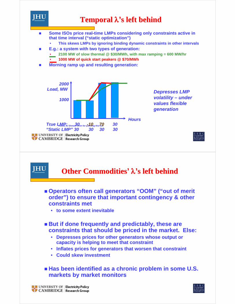
JHU___ Temporal Temporal λλ’’s left behinds left behind

Some ISOs price real-time LMPs considering only constraints active in that time interval (“static optimization”)• This skews LMPs by ignoring binding dynamic constraints in other intervals

E.g.: a system with two types of generation: • 2100 MW of slow thermal @ $30/MWh, with max ramping = 600 MW/hr• 1000 MW of quick start peakers @ $70/MWh

Morning ramp up and resulting generation:

• Kudos to Shmuel Oren for pointing this out

2000Load, MW

1000

HoursTrue LMP: 30 -10 70 30

Depresses LMPvolatility – undervalues flexiblegeneration

“Static LMP” 30 30 30 30

4444

JHU___ Other CommoditiesOther Commodities’’ λλ’’s left behinds left behind

Operators often call generators “OOM” (“out of merit order”) to ensure that important contingency & other constraints met• to some extent inevitable

But if done frequently and predictably, these are constraints that should be priced in the market. Else:• Depresses prices for other generators whose output or

capacity is helping to meet that constraint• Inflates prices for generators that worsen that constraint• Could skew investment

Has been identified as a chronic problem in some U.S. markets by market monitors

4545

JHU___ NonconvexNonconvex Costs: What are the Right Costs: What are the Right λλ’’s?s?

Common situation:• Cheap thermal units can continuously vary output• Costly peakers are either “on” or “off”⇒ Even during high loads, LMP set by cheap generators⇒ Too little incentive to reduce load⇒ Peakers don’t cover their costs (“uplift” required)⇒ Cheap units may get inadequate incentive to invest

California, New York solutions:• If peaking units are small relative to variation in load, • … then set LMP = average fuel cost of peaker, if peakers running• Note: LMP doesn’t “support” thermal unit dispatch, so must constrain output

Alternative: “Supporting prices” in mixed integer programming • Calculated from LP that constrains {0,1} variable to optimal level• Results in separate prices for supply (thermal plant MC) and demand (higher

LMP), and uplifts to peakers• Source: R. O’Neill, P. Sotkiewicz, B. Hobbs, M. Rothkopf, and W. Stewart, “Efficient Market-Clearing Prices

in Markets with Nonconvexities,” Euro. J. Operational Research, 164(1), July 1, 2005, 269-285

4646

JHU___ 5. Remaining Problems:5. Remaining Problems:b. Dealing With Market Powerb. Dealing With Market Power

Arises from:• Inelastic demand / inefficient pricing

• Scale economies

• Transmission constraints

• Dumb market designs

4747

JHU___ Mark Twain:Mark Twain:

“The researches of many commentators have already thrown much darkness on the subject and it is probable that, if they continue, we shall soon know nothing at all about it”

(thanks to Dick O’Neill for the quote)

4848

JHU___How to Respond?How to Respond?

Local Market Power Mitigation QuestionsLocal Market Power Mitigation Questions

Who is eligible for mitigation?

What triggers mitigation?

How much Q is mitigated?

What is the mitigated bid?

How are locational marginal prices (LMPs) calculated?

What is the bidder paid?

What if the bidder doesn’t cover its fixed costs?

stop

4949

JHU___ Various AnswersVarious Answers

Who is eligible for mitigation?• Everyone

• Congested areas / load pockets only. How to define?

What triggers mitigation?• Pivotal bidder (CAISO MSC [Wolak], Rothkopf)

• Out-of-merit order (PJM)

• Automated Mitigation Procedure (NYISO, NEISO, MISO)

– Conduct threshold (e.g., 200% over baseline bid)

– Impact threshold (e.g., raise market price by 50%)

5050

JHU___

How much Q is mitigated?• Entire capacity (PJM)

• Only pivotal/out-of-merit order quantity (California proposals)

What is the mitigated bid?• Baseline (mean bid during competitive period, plus negotiated

“hockey stick”) (MISO)

• Estimated variable cost (fuel only? maintenance?) (CAISO, PJM)

• Combustion turbine proxy (NEISO)

5151

JHU___

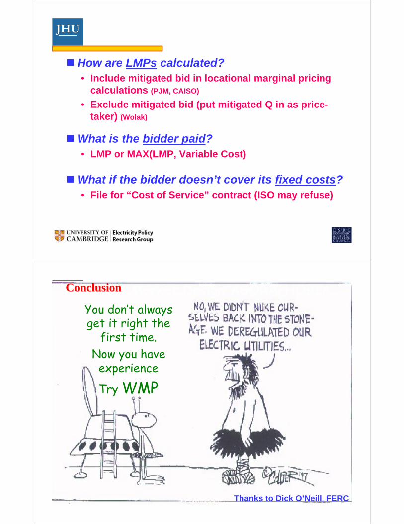
How are LMPs calculated?• Include mitigated bid in locational marginal pricing

calculations (PJM, CAISO)

• Exclude mitigated bid (put mitigated Q in as price-taker) (Wolak)

What is the bidder paid?• LMP or MAX(LMP, Variable Cost)

What if the bidder doesn’t cover its fixed costs? • File for “Cost of Service” contract (ISO may refuse)

5252

JHU___You don’t always get it right the

first time.Now you have experience

Try WMP

Wholestic Market Design AGORAPHOBIA

Thanks to Dick O’Neill, FERC

ConclusionConclusion

5353

JHU___

Questions?Questions?

5454

JHU___

CAISO MRTU trainingLocational Marginal Pricing (LMP) 101 Course Overview of Locational Marginal Pricinghttp://www.caiso.com/1824/18249c7b59690.html

http://www.caiso.com/20a6/20a690af67c80.html slides only

New Englandhttp://www.iso-ne.com/nwsiss/grid_mkts/how_mkts_wrk/lmp/index.html

PJM Training Curriculumhttp://www.pjm.com/sitecore/content/Globals/Training/Courses/ol-lmp-101.aspx?sc_lang=enhttp://www.pjm.com/~/media/training/core-curriculum/ip-lmp-101/lmp-101-training.ashxhttp://www.pjm.com/~/media/training/core-curriculum/ip-gen-101/20050713-gen-101-lmp-overview.ashxhttps://admin.acrobat.com/_a16103949/p20016248/ with audio accompaniment

ISO LMP Training MaterialsISO LMP Training Materials

5555

JHU___

AnswersAnswers

5656

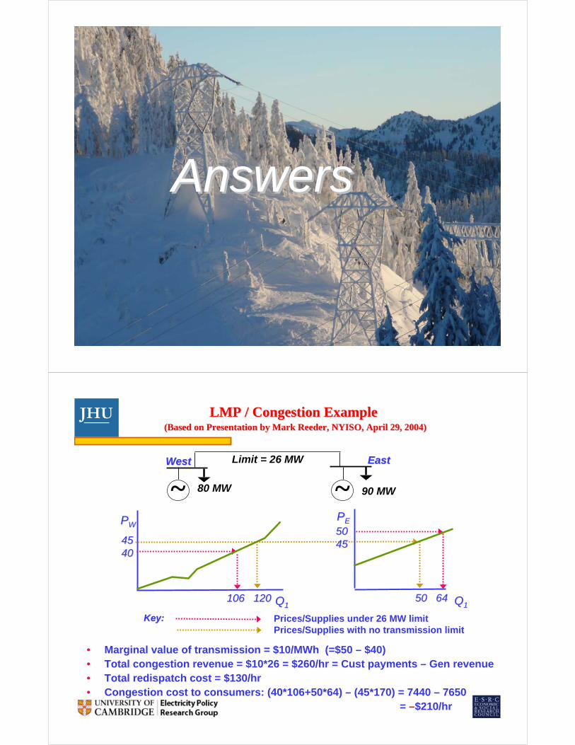
JHU___ LMP / Congestion ExampleLMP / Congestion Example(Based on Presentation by Mark Reeder, NYISO, April 29, 2004)(Based on Presentation by Mark Reeder, NYISO, April 29, 2004)

• Marginal value of transmission = $10/MWh (=$50 – $40)• Total congestion revenue = $10*26 = $260/hr = Cust payments – Gen revenue • Total redispatch cost = $130/hr• Congestion cost to consumers: (40*106+50*64) – (45*170) = 7440 – 7650

= –$210/hr

~WestWest EastEast

~Limit = 26 MW

80 MW 90 MW

PPWW

QQ11106 120106 120

45454040

QQ1150 6450 64

50504545

PPEE

Key:Key: Prices/Supplies under 26 MW limitPrices/Supplies with no transmission limit

5757

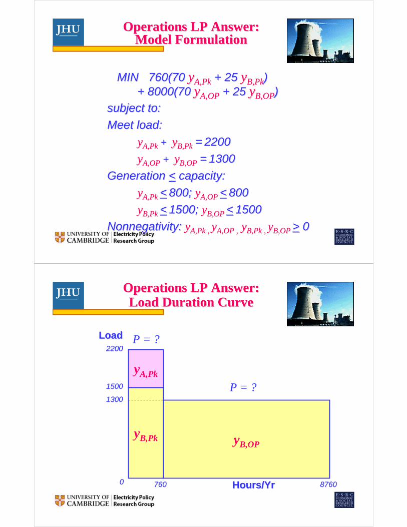
JHU___ Operations LP Answer:Operations LP Answer:Model FormulationModel Formulation

MIN 760(70 MIN 760(70 yyA,PkA,Pk + 25 + 25 yyB,PkB,Pk))+ 8000(70 + 8000(70 yyA,OPA,OP + 25 + 25 yyB,OPB,OP))

subject to:subject to:

Meet load:Meet load:

yyA,PkA,Pk + + yyB,PkB,Pk == 22002200

yyA,OPA,OP + + yyB,OPB,OP == 13001300

Generation Generation << capacity:capacity:

yyA,PkA,Pk << 800; 800; yyA,OPA,OP << 800800

yyB,PkB,Pk << 1500; 1500; yyB,OPB,OP << 1500 1500

NonnegativityNonnegativity: : yyA,PkA,Pk , , yyA,OPA,OP ,, yyB,PkB,Pk , , yyB,OPB,OP >> 00

5858

JHU___Operations LP Answer:Operations LP Answer:Load Duration CurveLoad Duration Curve

yB,Pk

yA,Pk

yB,OP

LoadLoad

Hours/YrHours/Yr

22002200

15001500

1300 1300

0 0 760 760 87608760

P = ?

P = ?

5959

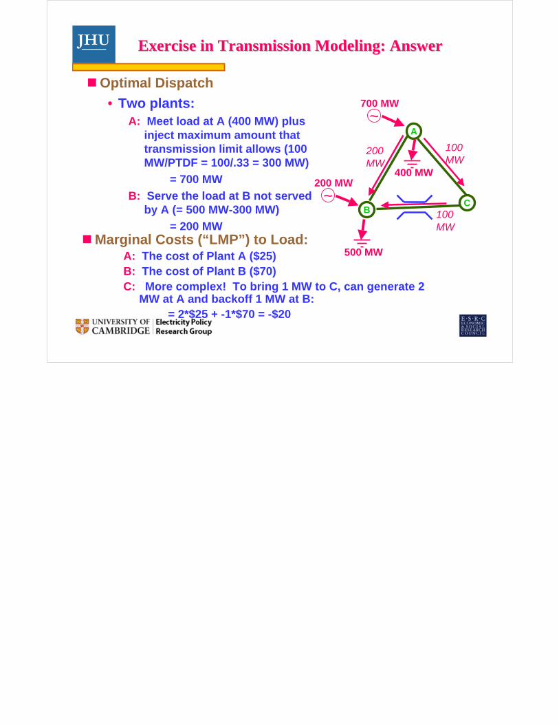
JHU___ Exercise in Transmission Modeling: AnswerExercise in Transmission Modeling: Answer

Optimal Dispatch

• Two plants: A: Meet load at A (400 MW) plus

inject maximum amount that transmission limit allows (100 MW/PTDF = 100/.33 = 300 MW)

= 700 MW

B: Serve the load at B not served by A (= 500 MW-300 MW)

= 200 MW

A

BC

~700 MW

400 MW

~200 MW

500 MWMarginal Costs (“LMP”) to Load:

A: The cost of Plant A ($25)B: The cost of Plant B ($70)C: More complex! To bring 1 MW to C, can generate 2

MW at A and backoff 1 MW at B:= 2*$25 + -1*$70 = -$20

100MW

200MW

100MW