Tasmanian School of Business and Economics University of Tasmania

Discussion Paper Series N 2015‐08

Oil Prices and Global Factor Macroeconomic

Variables 

Ronald RATTI University of Western Sydney

Joaquin VESPIGNANI University of Tasmania

   

ISBN 978‐1‐86295‐833‐3 

1  

Oil prices and global factor macroeconomic variables

Ronald A. Rattia and Joaquin L. Vespignanib**

aUniversity of Western Sydney, School of Business, Australia and Centre for Applied Macroeconomic Analysis, Australia

bUniversity of Tasmania, Tasmanian School of Business and Economics, Australia

Centre for Applied Macroeconomic Analysis. Australia and Globalization & Monetary Policy Institute, Federal Reserve Bank of Dallas, USA

Abstract

This paper investigates the relationship between oil prices, and global output, prices, central bank policy interest rate and monetary aggregates with a global factor-augmented error correction model. We confirm the following stylized relationships: i) in line with the quantitative theory of money, at global level, money, output and prices are cointegrated; ii) positive innovation in global oil price is connected with global interest rate tightening; iii) positive innovation in global money, price level and output is connected with an increase in oil prices; iv) positive innovations in global interest rate are associated with a decline in oil prices; v) positive shocks to the trade weighted U.S. dollar are linked with reductions in oil price; vi) the U.S., Euro area and China are the main drivers of global macroeconomic factors. Keywords: Global interest rate, global monetary aggregates, oil prices, GFAVEC

JEL Codes: E44, E50, Q43

*Ronald A. Ratti; University of Western Sydney, School of Business, Australia; Tel. No: +61 2 9685 9346; E-mail address: r.ratti@uws.edu.au **Corresponding author: Joaquin L. Vespignani; University of Tasmania, School of Economics and Finance, Australia; Tel. No: +61 3 62262825; E-mail address: Joaquin.Vespignani@utas.edu.au

2  

Oil prices and global factor macroeconomic variables

1. Introduction

Since the mid-1990’s several important changes took place in the global economy and

the international oil market. With the creation of the ECB in 1999 and the fast economic

growth undertaking by China and India, the largest 5 economies (the Euro area, the U.S.,

China Japan and India) now account for around 65% of the world economy (measured in

purchase power parity) and global demand for oil in recent decades has been driven by rapid

growth in major developing economies.1 Important changes have also occurred in the global

economy in terms of central bank actions. With many countries suffering prolonged

economic downturns and official/policy interest rates being close to zero, after the global

financial crisis in 2008, the U.S., Japan, Euro area and the U.K. central banks have turned to

alternative policies to expand monetary aggregates and hence stimulate the economy.

The literature generally analyses the relationship between the U.S. federal funds rate

and oil prices. However, in the current context we believe that central bank interest rates at

global level and also global monetary aggregates should be considered in interaction with oil

prices, particularly given the surge in the Chinese and Indian economies and the new ways

that central banks now seek to influence the economy.

The US Energy Information Agency documents that China became the world's largest

net importer of oil on an annual basis in 2014. The largest oil consuming countries in 2014

are the US, China, Japan and India in that order. India has increased oil consumption by over

                                                            1 Kilian and Hicks (2013) connect real oil price increases with strong growth forecasts in emerging economies (especially in China and India) over 2003-2008 and the decline in real oil prices after mid 2008 with forecasts of decline in global growth. Beirne et al. (2013) estimate the effects of individual countries on oil demand and find that China’s GDP growth attaches a premium to the price of oil that is rising over time.  Hamilton (2013) notes that the newly industrialized economies have absorbed over two-thirds of the increase in world oil consumption since 1998. Cagliarini and McKibbin (2010) emphasize that growth in emerging economy countries has boasted commodity prices in recent years.

3  

50% over 2000-2010. The surge in demand for oil by China and India is forecasted by the

IEA to continue well into the future.2

While growth in emerging economies has mattered primarily for the latest surge in oil

prices; more generally, this is about demand from all countries in the world. Barsky and

Kilian (2004) emphasize that oil prices are endogenous with respect to U.S. and global

macroeconomic conditions.3 It is also stressed that the behaviour of commodity prices is

closely intertwined with global monetary conditions. Barsky and Kilian (2002) show that the

global shifts in monetary policy regimes in the 1970s caused shifts in real economic growth

and inflation and hence in the real price of oil. Bodenstein, Guerrieri and Kilian (2012)

develop a DSGE model and argue that causality runs from the oil market to monetary policy

as well as from changes in monetary policy to the supply and demand of oil in global

markets. Belke, Bordon and Hendricks (2010) find that causality between global monetary

aggregates and oil price runs both ways. The literature is clear that when considering the

world price for oil it is necessary to consider the influence of global variables, including

global variables that reflect the stance of monetary policy in the major developing and

developed countries.

We believe that this paper contributes to the literature by providing stylized facts on

the interaction between oil prices and factor augmented global macroeconomic variables,

including aggregated central bank policy interest rates and liquidity. A factor-augmented

dimension to the GFAVEC model will capture the dynamic of the information provided by

many variables to the analysis of short and long run interaction of global oil price, global real

output, global CPI and global policy interest rate. Global factors are estimated using principal

                                                            2 The IEA projects that “China, India, and the Middle East will account for 60% of a 30% increase in global energy demand between now and 2035”… “By 2035, almost 90% of Middle Eastern oil flows to Asia” (IEA World Energy Outlook 2012: http://www.worldenergyoutlook.org/pressmedia/quotes/12/ ). 3 Recent work on global influence on the price of oil include Kilian and Lee (2014) and Kilian and Murphy (2014) investigating the roles of speculation and inventories in influencing the price of oil. 

4  

component techniques applied to interest rates, real output across countries, and CPI across

countries, respectively. 4

Use of factor analysis for crude oil prices is appropriate for analysis of the behaviour

of the global economy since Brent and West Texas Intermediate (WTI) crude oil price data

have diverged sharply in recent years. Prior to the global financial crisis (GFC) the WTI

crude oil price usually exceeded the Brent by at most a few dollars per barrel, but since the

GFC Brent crude oil price has occasionally topped WTI crude oil price by $28 per barrel. A

global factor for oil price better captures the movement in oil price relevant for the global

economy than do the individual prices for Brent, WTI and Dubai oil.

Some stylized facts that emerge from our empirical analysis are:

i) Global money, global output and global prices are found to be cointegrated, consistent with

the quantity theory of money holding at global level.  

ii) Granger causality goes from liquidity to oil prices and from oil prices to the global interest

rate, global output and global CPI.

iii) Positive innovations in world oil price are connected with statistically significant

extended positive effects on global interest rates and global real output.

vi) Positive shock in world oil price is linked with a statistically significant decline in the

trade weighted value of the US dollar.

v) Positive innovation in the global interest rate leads to statistically significant and persistent

decreases in global oil price.

vi) Statistically significant persistent increases in global oil price are associated with positive

shocks to global M2, to global CPI and to global real output, and to negative innovations in

the trade weighted value of the US dollar.

                                                            4 It is emphasized that this is not the same as the stance of global monetary policy since there is no global central bank. In recent years the effect of global liquidity on the prices of commodities has been emphasized by some researchers. Increases in liquidity raise aggregate demand and thereby increase commodity prices.  

5  

The methodology and global variable are described in Section 2. Granger causality

among the economic variable and global macroeconomic variables is investigated in Section

3. The GFAVEC model is presented in Section 4. The empirical results are presented in

Section 5. The robustness of results to alternative definitions of the variables and different

model specifications is discussed in Section 6. Section 7 concludes.

2. Data and global factors

2.1. Background

Factor methods have become widely used in the literature to examine the co-

movements of aggregate variables since work by Stock and Watson (1998) and Forni et al.

(2000).5 In line with the dynamic factor models of Bernanke et al. (2005), Stock and Watson

(2005), Forni and Gambetti (2010), and others, we construct a global factor-augmented error

correction model to examine the relationships between oil prices, global interest rate, global

monetary aggregates, global real output and global CPI and the weighted trade index of the

US dollar. A cointegrating vector for global money, global real output and global price level

is utilized.

The main advantage of this approach in a global setup is that it is possible to compress

data for many countries in single factor without losing degrees of freedom, allowing for the

influence of both large developed and developing economies. A single individual variable or

                                                            5A number of issues have been addressed recently using factor methods. Building on Stock and Watson (2002), Bernanke et al. (2005) propose a Factor-augmented VAR (FAVAR) to identify monetary policy shocks. Mumtaz and Surico (2009) extend Bernanke et al. (2005) to consider a FAVAR for an open economy. A factor-augmented approach has been used by Dave et al. (2013) to isolate the bank lending channel in monetary transmission of US monetary policy and by Gilchrist et al. (2009) to assess the impact of credit market shocks on US activity. Le Bihan and Matheron (2012) use principal components to filter out sector-specific shocks to examine the connection between stickiness of prices and the persistence of inflation. Boivin et al. (2009) assume that the connection between sticky prices and monetary policy can be captured by five common factors estimated by principal component analysis. Abdallah and Lastrapes (2013) use a FAVAR model to examine house prices across states in the US. Beckmann et al. (2014) examine the effect of global shocks on policy making for the US, Euro area, Japan, UK and Canada. Juvenal and Petrella (2014) in an examination of the role of speculation in the oil market, construct a factor for speculation based on a large number of macroeconomic and financial variables for the G7.

6  

factor can capture the dynamic of a large amount of information contained in many

variables.6

2.2. The Data.

The data are monthly from January 1999 to December 2013. The starting period

coincides with the creation of the European Central Bank and data on CPI and interest rate

for this block is only available from January 1999. Monthly data is used to overcome the

limitation of few observations obtained from quarterly data over a 13 year period. Data are

obtained on the central bank discount rate, monetary aggregate M2, consumer price index,

and industrial production index for each of the five largest economies given by the Euro area,

the US, Japan, China and India. Oil prices are given by the Brent, Dubai and West Texas

Intermediate US dollar international indexes for crude oil prices. The trade weighted index

for the US dollar completes the data.7 Data on each country are from the Federal Reserve of

St. Louis (FRED data) and data on oil prices are from the World Bank.

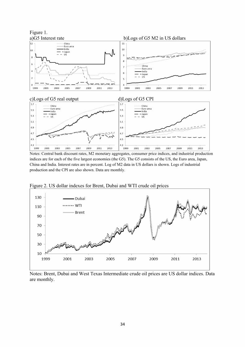
Information on the interest rate, liquidity (measure by M2 in US dollars), CPI and real

output for the US, Euro area, China, India, and Japan over 1999:01-2013:12 are shown in

Figure 1. The central bank discount rate for each of the five economies has varied over time.

Although at widely different levels, the interest rates all show declines following the March-

November 2001 recession in the US. With the exception of India, central bank discount rate

register increases during the commodity price boom over 2005-2008 and fall during the

global financial crises. Liquidity (M2 in US dollars) increases over the fourteen years from

1999:01 to 2013:12 by approximately a factor of 12 in China, 4.8 in India, 2.3 in the US, 2.6

in Euro area, and by 2 in Japan.                                                             6 Sims (2002) argues that when deciding policy central banks consider a huge amount of data.  An overview of factor-augmented VARs and other models is provided by Koop and Korobilis (2009). Boivin and Ng (2006) caution that expansion of the underlying data could result in factors less helpful for forecasting when idiosyncratic errors are cross-correlated or when a useful factor in a small dataset becomes dominated in a larger dataset. 7 Major currencies index from the Federal Reserve System of the United State includes: the Euro Area, Canada, Japan, United Kingdom, Switzerland, Australia, and Sweden. Weights are discuss in: http://www.federalreserve.gov/pubs/bulletin/2005/winter05_index.pdf  

7  

The consumer price level is  up by a factor of 1.34 in China, 2.4 in India, 1.4 in the

US, 1.35 in Euro area, and down by 4% in Japan. Compared to the US, the Euro area and

Japan, China and India have grown much faster in recent years. For example, over the

fourteen years from 1999:01 to 2013:12 real output is up approximately by factors of about

2.9 and 2.3 in China and India, respectively, and up by only about 14% and 6% in the US and

the Euro area, respectively, and down by about 3% in Japan.  On the basis of GDP in

purchasing power parity in 2013 (in declining order) the US, Euro area, China, India, and

Japan, are by far and away the largest economies in the world.

2.3. The global factors

Principal components indexes are constructed for each group of variables for the five

economies. These are global factors for the global interest rate , global CPI

and global real output .8 A global money monetary aggregate M2 2 , the sum of

M2 monetary aggregates across economies (in US dollars), captures the effect of liquidity.

Global oil prices (GOP), is constructed by using a unique principal component index based

on information for the Brent, Dubai and West Texas Intermediate US dollar based

international indexes for crude oil prices.

The indicators of global interest rate, global real output and of global CPI are the

leading principal components for interest rates, real output and CPI (in log-level form for real

output and CPI) of the US, Euro area, China, India, and Japan. These are given by

, , , , , (1)

, , , , , (2)

, , , , , (3)

where the superscripts Ea, US, Ch, Ja, and In, represent the Euro area, US, China, Japan, and

India, respectively, in equations (1), (2) and (3). In equation (1), is a vector containing

                                                            8 Industrial production is used as a measure of country’s real output.  

8  

the discount rate of the central banks of the Euro area, US, China, Japan and India. 9

Equations (2) and (3) are vectors containing the real output and CPI for the same economies,

respectively.10

The indicator for global oil prices is the leading principal component of the Dubai,

Brent and West Texas Intermediate oil prices and is given by

, , (4)

A global factor for oil price better captures movement oil price relevant for the global

economy than the individual prices for Brent, Dubai and WTI oil. US dollar indexes for

Brent, Dubai and WTI crude oil prices are shown in Figure 2. Before the GFC, the WTI and

Brent crude oil prices were within a couple of dollars of each other, with WTI usually at a

premium relative to Brent. Since 2011, WTI has traded at a significant discount to Brent and

on September 21, 2011, the discount achieved $28.49 per barrel. The price gap between Brent

and Dubai also fluctuates. Before 2011, Brent crude oil typically traded at a one or two dollar

premium relative to Dubai crude oil. The premium for Brent over Dubai surged to $7.60 per

barrel in 2011 with the crisis in Libya, before falling to a low of $1.1 per barrel in November

2012, and surging again to almost $6 per barrel in August 2013. Movement in these price

gaps reflect changes in the market conditions in various parts of the world driven by

economic and political considerations.11

                                                            9 Structural factors in VAR models to better identify the effects of monetary policy have appeared in a number of contributions (for example, by Belviso and Milani (2006), Laganà (2009) and Kim and Taylor (2012), amongst others), but less so in work on commodity prices. An exception is by Lombardi et al. (2012) examining global commodity cycles in a FAVAR model in which factors represent common trends in metals and food prices. 10 The first principal component for country CPIs to indicate global inflation is similar to Ciccarelli and Mojon (2009) method of identifying global inflation based on price indices for 22 OECD countries and a factor model with fixed coefficients. Within the factor analysis framework, a different approach is taken by Mumtaz and Surico (2012) who derive factors representing global inflation from a panel of 164 inflation indicators for the G7 and three other countries. 11 WTI represents the price oil producers receive in the U.S. and Brent and Dubai represents the prices received internationally. The WTI and Brent crude oils share a similar quality and Dubai has higher sulphur. The recent negative premium for WTI relative to Brent is usually explained in terms of oil production in the US exceeding cheap transportation capacity by pipeline to refiners on the US Gulf Coast. Fluctuation in the premium for Brent over Dubai is usually tied to political events in North Africa and the Middle East.

9  

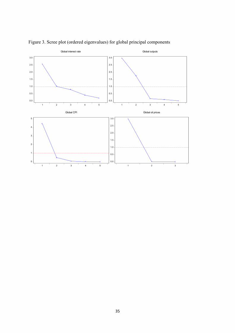
Figure 3 contains a plot of the variance of the principal components using normalised

loadings for the interest rate, real output, CPI and oil price. Each plot for shows the variance

accounted for by the first component and then for the second, third etc. components for each

variable. The first principle component for each variable captures most of the variation in

each variable across the five economies (for the interest rate, real output and CPI) and the

three oil price indices. For the global CPI and global oil price, in particular, the first principal

components capture nearly all of the information in the five economy level consumer price

indices (88%) and the three oil price indices (99%). The first principal component for interest

rates (output) captures 60% (46%) of the news in the five economy level interest rates

(output). We use one factor (the principal component) for the global interest rate, global real

output global CPI, and global oil price to keep the total number of variables in the estimation

of the global relationship to a minimum.

Alternative principal components can also be derived from the equations (1) through

(4). These alternatives are: normalise loadings (where the variance is equal to the estimated

eigenvalues; normalise scores (with unit variances with symmetric weights); and with equal

weighted scores and loadings. The representation for equal weighted scores and loadings falls

in between those for normalise loadings and normalise scores. In the basic model

constructing principal components we will use normalise loadings and consider use of

normalise scores in a section on the robustness of results.12 The first principal component for

the global interest rate, to be referred to as , is drawn in Figure 4a for normalise

loadings, normalise scores, and with equal weighted scores and loadings. It captures the fall

in interest rates at the end of 2008 with the onset of the global financial crisis as well as the

                                                            12 Note that with normalise loading option more weight is given to variables (countries in this case) with higher standard deviation. With scores options all the variables are given equal weight (by standardising them). The direct implication in this study by choosing normalise loading is that more weight is given to developing economies which generally have higher standard deviation in this sample. This a desirable future of this option considering the views of Hamilton (2009; 2013) and Kilian and Hicks (2013) that for the period of analysis oil prices are largely influenced by the surge in growth in developing economies.

10  

fall in interest rates during and following the 2001 recession in the US. The first principal

component for the CPI indices, , is shown in Figure 4b. In Figure 4 slopes

upward. The slight concavity in the curve over 2000-2006 indicates higher CPI over this

period followed by an overall flat rate of inflation in the last half of the sample.

The first principal component for global real output, , is represented in Figure 4c.

Global real output has an upward trend until the global financial crisis in 2008. There is a

severe correction in in 2008-2009, reflecting the global financial crisis, with recovery of

global real output to early 2008 levels only in 2011. Global real output also shows a

correction in 2001 coinciding with the March-November 2001 recession in the US. The

principle component for crude oil prices is shown in Figure 4d. Oil price rose sharply from

January 2007 to June 2008. Concurrent with the global financial crisis and the weak global

economy the oil price fell steeply until January 2009 before substantially rebounding over the

next few years. The log of the trade weighted index of the US dollar is shown in Figure 4e.

The trade weighted US dollar peaks in early 2002 and then shows a gradual downward with a

levelling off in recent years. The log of global M2 is shown in Figure 4f and shows an

upward trend.

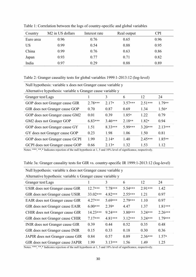
Information on the correlations between country-specific and global factor for M2,

short-term interest rate, real output and CPI are reported in the columns in Table 1. The

global factors are given by first principal components for global M2, the global interest rate

(GIR), global real output (GY), and global CPI (GCPI). The global M2 is highly correlated

with M2 in each of the five economies. The global interest rate correlation with country

interest rates is high for the Euro area, China and Japan (over 75% for each), 54% for the US

and only 29% for India. The global real output correlation with country level real output is

high for the US and India (88% each), and at 71%, 65% and 63% for Japan, Euro area and

11  

China, respectively. The global CPI correlation is high with that of each economy with

correlations at 82% and above.

3. Causality tests

We now examine the direction of causality between the variables at global level and

also the causality between the developed and developing large economies and the variables at

global level. The issue of causality between global variables and global oil price is not

usually addressed in the literature, but is clearly of interest given the increased

interconnectedness of the world economy. Work on the impact of a large economy on other

economies has naturally focused on the role of the US in the international transmission of

shocks.13 China and India are now a large economies and their impact on global variables

needs to be examined along with that of the US, Euro area and Japan.

3.1 Directional influence amongst global variables.

In Table 2 the Granger causality direction results for the global interest rate, global

M2, global output and global CPI with global oil price are presented. The balance of the

evidence is that global oil price Granger causes global interest rate, global output and global

CPI, and not the reverse of these outcomes. These results supplement the large literature

assigning oil price shock a major role in influencing real activity in individual economies by

suggesting that even global variables are influenced by oil prices.  Hamilton’s (1983)

influential paper on the effect of oil prices on the US economy over the post-World War II

period treated oil prices changes as exogenous. This supposition was maintained by Lee et al.

(1995), Hamilton (1996) and Bernanke et al. (1997), among many others, who documented a

                                                            13 With regard to monetary policy, Kim (2001) and Canova (2005) find that monetary expansion in the US causes economic expansion in the non-US G-6 and in Latin America by lowering interest rates across these economies.

12  

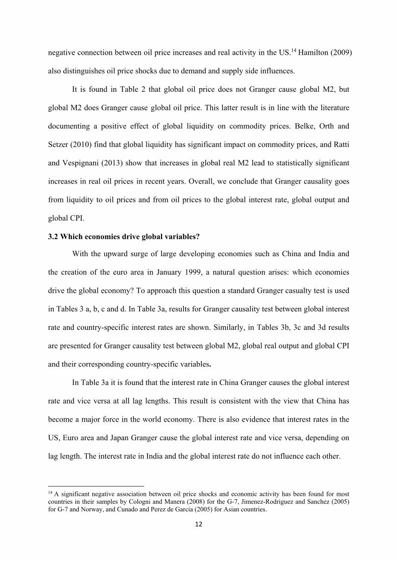
negative connection between oil price increases and real activity in the US.14 Hamilton (2009)

also distinguishes oil price shocks due to demand and supply side influences.

It is found in Table 2 that global oil price does not Granger cause global M2, but

global M2 does Granger cause  global oil price. This latter result is in line with the literature

documenting a positive effect of global liquidity on commodity prices. Belke, Orth and

Setzer (2010) find that global liquidity has significant impact on commodity prices, and Ratti

and Vespignani (2013) show that increases in global real M2 lead to statistically significant

increases in real oil prices  in recent years. Overall, we conclude that Granger causality goes

from liquidity to oil prices and from oil prices to the global interest rate, global output and

global CPI.

3.2 Which economies drive global variables?

With the upward surge of large developing economies such as China and India and

the creation of the euro area in January 1999, a natural question arises: which economies

drive the global economy? To approach this question a standard Granger casualty test is used

in Tables 3 a, b, c and d. In Table 3a, results for Granger causality test between global interest

rate and country-specific interest rates are shown. Similarly, in Tables 3b, 3c and 3d results

are presented for Granger causality test between global M2, global real output and global CPI

and their corresponding country-specific variables.

In Table 3a it is found that the interest rate in China Granger causes the global interest

rate and vice versa at all lag lengths. This result is consistent with the view that China has

become a major force in the world economy. There is also evidence that interest rates in the

US, Euro area and Japan Granger cause the global interest rate and vice versa, depending on

lag length. The interest rate in India and the global interest rate do not influence each other.

                                                            14 A significant negative association between oil price shocks and economic activity has been found for most countries in their samples by Cologni and Manera (2008) for the G-7, Jimenez-Rodriguez and Sanchez (2005) for G-7 and Norway, and Cunado and Perez de Garcia (2005) for Asian countries.

13  

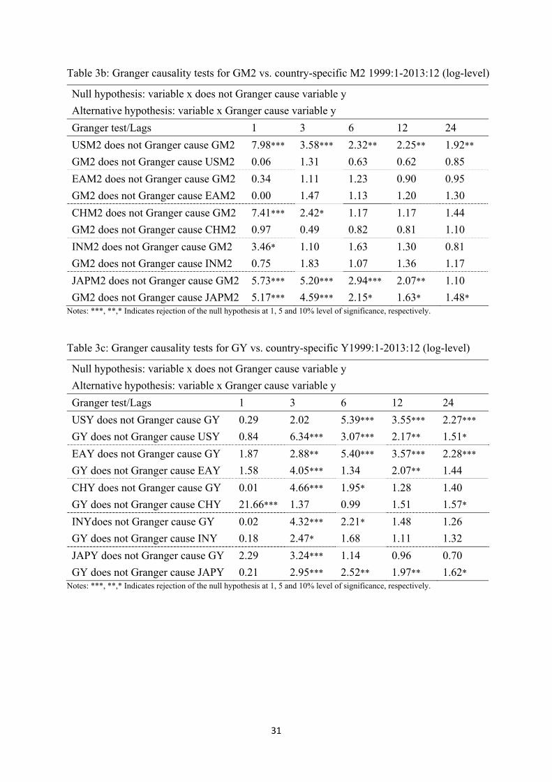
In Table 3b it is found that global M2 is Granger caused by M2 in China, Japan and

the US. Only Japan’s M2 Granger causes global M2. Global output is driven by output in all

five economies (with the US and Euro area having stronger results). Global output Granger

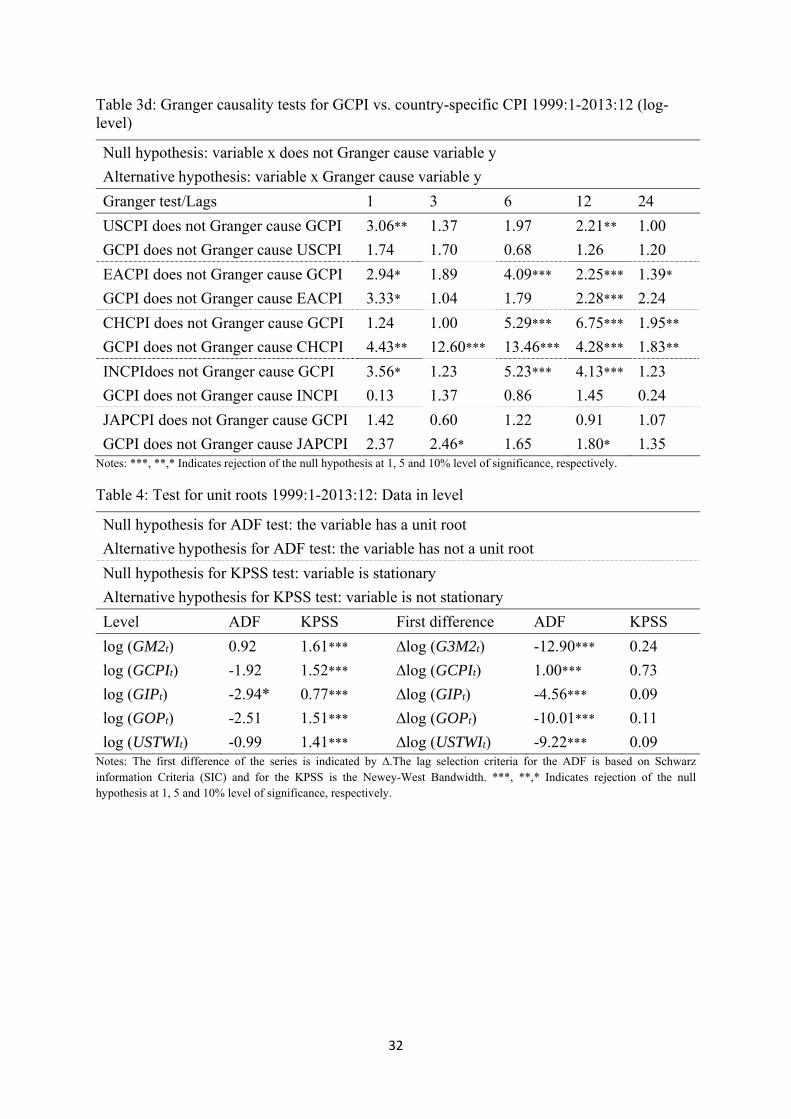
causes output in the US, Euro area, China and Japan. Global inflation is driven by inflation in

the US, Euro area, China and India, but not by inflation in Japan. Inflation in China and the

Euro area is Granger caused by global inflation.

In summary, the results indicate that the US and China have most breadth of influence

across the global variables for interest rate, liquidity, output and consumer prices. It is found

that in terms of Granger causality the US and China influence the global interest rate, global

M2, global output and global CPI. The Euro area influences the global interest rate, global

output and global CPI (but not global M2). Japan influences global M2 and global output (but

not the global interest rate and global CPI). India influences global output and global CPI (but

not global interest rate and global M2), suggesting that India is most divorced from the global

economy at least in terms of the financial variables (GIR and GM2). All five economies

influence global output. The results indicate a degree of interdependence between China and

the global economy that is similar to levels of interdependence between the global economy

and either the US, Euro area, or Japan.

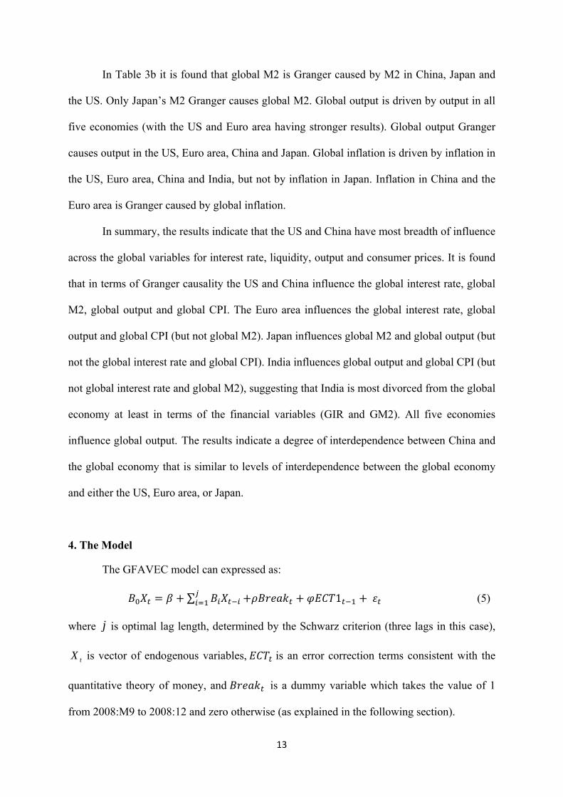
4. The Model

The GFAVEC model can expressed as:

∑ 1 (5)

where j is optimal lag length, determined by the Schwarz criterion (three lags in this case),

tX is vector of endogenous variables, is an error correction terms consistent with the

quantitative theory of money, and is a dummy variable which takes the value of 1

from 2008:M9 to 2008:12 and zero otherwise (as explained in the following section).

14  

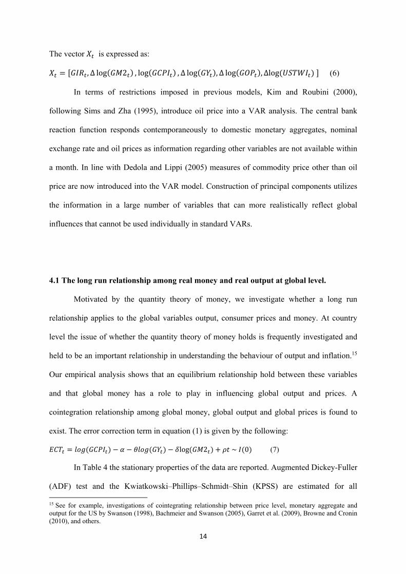
The vector is expressed as:

, ∆ log 2 , log , ∆ log , ∆ log , ∆log (6)

In terms of restrictions imposed in previous models, Kim and Roubini (2000),

following Sims and Zha (1995), introduce oil price into a VAR analysis. The central bank

reaction function responds contemporaneously to domestic monetary aggregates, nominal

exchange rate and oil prices as information regarding other variables are not available within

a month. In line with Dedola and Lippi (2005) measures of commodity price other than oil

price are now introduced into the VAR model. Construction of principal components utilizes

the information in a large number of variables that can more realistically reflect global

influences that cannot be used individually in standard VARs.

4.1 The long run relationship among real money and real output at global level.

Motivated by the quantity theory of money, we investigate whether a long run

relationship applies to the global variables output, consumer prices and money. At country

level the issue of whether the quantity theory of money holds is frequently investigated and

held to be an important relationship in understanding the behaviour of output and inflation.15

Our empirical analysis shows that an equilibrium relationship hold between these variables

and that global money has a role to play in influencing global output and prices. A

cointegration relationship among global money, global output and global prices is found to

exist. The error correction term in equation (1) is given by the following:

log 2 ~ 0 (7)

In Table 4 the stationary properties of the data are reported. Augmented Dickey-Fuller

(ADF) test and the Kwiatkowski–Phillips–Schmidt–Shin (KPSS) are estimated for all                                                             15 See for example, investigations of cointegrating relationship between price level, monetary aggregate and output for the US by Swanson (1998), Bachmeier and Swanson (2005), Garret et al. (2009), Browne and Cronin (2010), and others.

15  

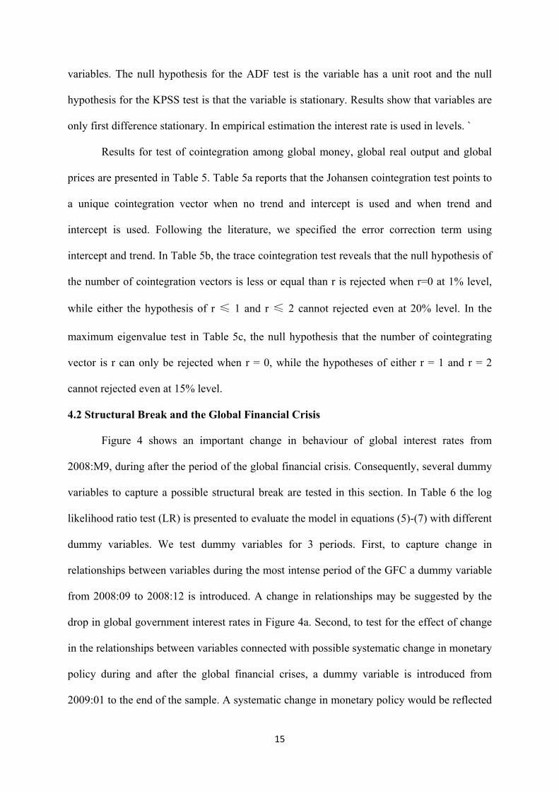
variables. The null hypothesis for the ADF test is the variable has a unit root and the null

hypothesis for the KPSS test is that the variable is stationary. Results show that variables are

only first difference stationary. In empirical estimation the interest rate is used in levels. `

Results for test of cointegration among global money, global real output and global

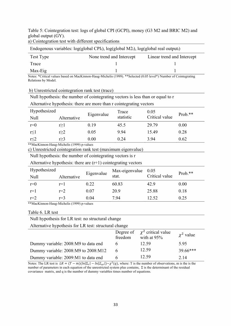
prices are presented in Table 5. Table 5a reports that the Johansen cointegration test points to

a unique cointegration vector when no trend and intercept is used and when trend and

intercept is used. Following the literature, we specified the error correction term using

intercept and trend. In Table 5b, the trace cointegration test reveals that the null hypothesis of

the number of cointegration vectors is less or equal than r is rejected when r=0 at 1% level,

while either the hypothesis of r ≤ 1 and r ≤ 2 cannot rejected even at 20% level. In the

maximum eigenvalue test in Table 5c, the null hypothesis that the number of cointegrating

vector is r can only be rejected when r = 0, while the hypotheses of either r = 1 and r = 2

cannot rejected even at 15% level.

4.2 Structural Break and the Global Financial Crisis

Figure 4 shows an important change in behaviour of global interest rates from

2008:M9, during after the period of the global financial crisis. Consequently, several dummy

variables to capture a possible structural break are tested in this section. In Table 6 the log

likelihood ratio test (LR) is presented to evaluate the model in equations (5)-(7) with different

dummy variables. We test dummy variables for 3 periods. First, to capture change in

relationships between variables during the most intense period of the GFC a dummy variable

from 2008:09 to 2008:12 is introduced. A change in relationships may be suggested by the

drop in global government interest rates in Figure 4a. Second, to test for the effect of change

in the relationships between variables connected with possible systematic change in monetary

policy during and after the global financial crises, a dummy variable is introduced from

2009:01 to the end of the sample. A systematic change in monetary policy would be reflected

16  

in quantitative easing in the developed countries discussed earlier. Thirdly, to capture the

effects of both the first two dummy variables, a dummy variable is introduced from 2008:09

to the end of the sample. This dummy variable captures systematic change that immediately

started with the initial shock of the GFC that continues beyond the crisis through to the

present.

Results in Table 6, shows that LR test rejects the null hypothesis of no structural

break at 1% significant level for the dummy variable from the period 2008:09 to 2008:12 (the

chi-square value is 39.66). The null hypothesis of no structural break for the dummy variables

from the periods 2008:09 to 2013:12 and from 2009:01 to 2013:12 cannot be rejected. In line

with these results we include a dummy variable, value 1 over 2008:09 to 2008:12 and 0

otherwise, in the model in equations (5) to (7).

5. Empirical results

The impact of shocks to variables in the GFAVEC model will be examined using

generalized cumulative impulse response (GIRF) developed by Koop et al. (1996) and

Pesaran and Shin (1998). Unlike conventional impulse response, generalized impulse

response analysis approach is invariant to the ordering of the variables which is an advantage

in absence of strong prior belief on ordering of the variables. Pesaran and Shin (1998) show

that the generalized impulse response coincides with a Cholesky decomposition when the

variable shocked is ordered first and does not react contemporaneously to any other variable

in the system.

The responses of variables in the GFAVEC model (in equations (5), (6) and (7)) to

one-standard deviation structural innovations are shown in Figure 5. The dashed lines

represent a one standard error confidence band around the estimates of the coefficients of the

17  

impulse response functions.16 The first row in Figure 5 shows the response of the global

interest rate to structural innovations in the global interest rate, global M2, global CPI, global

output, oil price, and the trade weighted US dollar exchange rate, in turn. Similarly, the

second, third, fourth, fifth and sixth rows show the response of global M2, global CPI, global

output, oil price, and the trade weighted US dollar exchange rate, respectively, to structural

innovations in , ∆ log 2 , ∆log , in ∆log , ∆ log , and

∆log in turn.

5.1. Response of global interest rate to structural shocks

It is not clear from the literature what the effects on global interest rates should be

from structural shocks to the global variables. The countries in the G5 have different

exchange rate regimes, capital controls and monetary policies. There is no global central bank

and the global interest represents the first principal component of the data on the discount

rates of the G5.

In the first row of Figure 5, a positive shock to global M2 is associated with a rising

global interest rate over time. This result is consistent with Thornton’s (2014) observation

that a liquidity effect is not observed at country level. Also in the first row of Figure 5,

positive shocks to global CPI, to global real output, and to oil price lead to statistically

significant and persistent increases in the global interest rate (in the third through fifth

diagrams in row 1).17 The results indicate that there is a general tightening of monetary policy

on a global level, as indicated by a rise in the global interest rate, when global level liquidity

is increasing, the economy is heating up in terms of rising output and prices, and oil prices

are rising.

                                                            16 The confidence bands are obtained using Monte Carlo integration as described by Sims (1980), where 5000 draws were used from the asymptotic distribution of the VAR coefficient. 17 Consistent with this finding, Mallick and Sousa (2013) report that commodity price shocks can result in an aggressive response from BRIC central banks concerned with inflation stabilisation.

18  

A positive shock to  the trade weighted value of the US dollar results in a significant

decline in the global interest rate in the sixth  diagram in row 1 of Figure 5. This result is in

harmony with Shin’s (2014) reasoning that a stronger US dollar constitutes a tightening of

global financial conditions that central banks might offset. The burden of dollar-denominated

debt repayment results in a tightening of global financial conditions when the US dollar rises.

Consistent with a rise in the US dollar being associated with more constrictive global

financial conditions (for given central bank interest rates) there is a rise in global M2 and

declines in CPI, real output and oil prices, for extended periods in response to a positive

shock to the trade weighted value of the US dollar in the last column of Figure 5.

5.2. Response of global variables to structural shock to global interest rate

In the first column of Figure 5, a positive shock to global interest rates leads to

statistically significant and persistent decline in global M2. Monetary tightening at global

level is connected with reduced CPI and nominal oil price, and after a positive bump to

reduced global output.18 In the second column of Figure 5, a positive shock to global M2 is

linked with increases in CPI and in nominal oil price, and after four months with increased

global output.

5.3. Liquidity and structural shocks

The second column in Figure 5 reports the effects on the global variables of a positive

structural shock to liquidity. Global liquidity significantly impacts global CPI 3 and 4 months

later. The impact on oil price is statistically significant after 3 months and remains so over the

20 month horizon. A positive innovation in global liquidity significantly impacts output over

a 5 to 13 month horizon. The trade weighted value of the US dollar declines with a positive

innovation in global M2 and the effect is immediate and persists over the entire horizon. In

                                                            18 In connection with monetary tightening being associated with a fall in oil price, Hammoudeh et al. (2015) using a structural VAR model and find that increases in the federal funds rate are associated with declines in energy prices.

19  

line with results in the literature, increases in global liquidity are associated with global

expansion and rising oil and global consumer prices.

5.4. The oil price and structural shocks

The impulse responses of oil price to global variables are presented in the fifth row of

Figure 5. A negative shock to global interest rates and positive shocks to global M2, to global

CPI, and to global real output, lead to statistically significant and persistent increases in

global oil price (in the first through fourth diagrams). A positive innovation in M2 supports a

higher level of spending with positive effects on nominal oil price. A positive shock in the

global CPI, reflects a negative shock to the real price of oil and an increase in oil price. A

positive innovation in global real output indicates a higher level of global real activity with

concomitant increases in the demand for crude oil and an increase in the global oil price.

In the fifth column of Figure 5, a positive innovation in oil price is associated with a

statistically significant positive effect on the global interest rate and on global real output.

Positive shocks to oil price have significant effects on global M2 and global CPI at impact

only.19 A negative shock in oil price leads to a statistically significant increase in the trade

weighted value of the US dollar. This latter result is consistent with the finding by Aloui et al.

(2013) that a rise in the price of oil is associated with the depreciation of the US dollar.

6. Robustness of results to alternative specifications

In this section the robustness of results to changing the definition of the global

variables, to alternative identification restrictions, and to different definitions of the principal

components is examined.

6.1. G8 economies

We now consider the robustness of results to expanding the analysis from the five

largest economies to the eight largest economies on GDP based on PPP basis. This means in

                                                            19 Valadkhani (2014) suggests that the relationship between oil price and the consumer price index has changed over time (for Canada and the U.S.)

20  

constructing principal components for the interest rate, output and inflation we add data on

these variables for Russia, Brazil and the U.K. to that for the US, Euro area, Japan, China and

India. Our first preference is to use data from the five largest economies because these

economies are much closer in size than when sixth, seventh and eights economies are

included (Russia, Brazil and the U.K. respectively). 20 However, the major developing

economies taken to be the BRIC countries, Brazil, the Russian Federation, India and China,

have dramatic increases in real income in recent years and their inclusion along with the

largest developed economies in an analysis of global effects of oil prices is a reasonable

robustness analysis. The global measure of M2 will now be the sum of M2 in the largest eight

economies in US dollars.

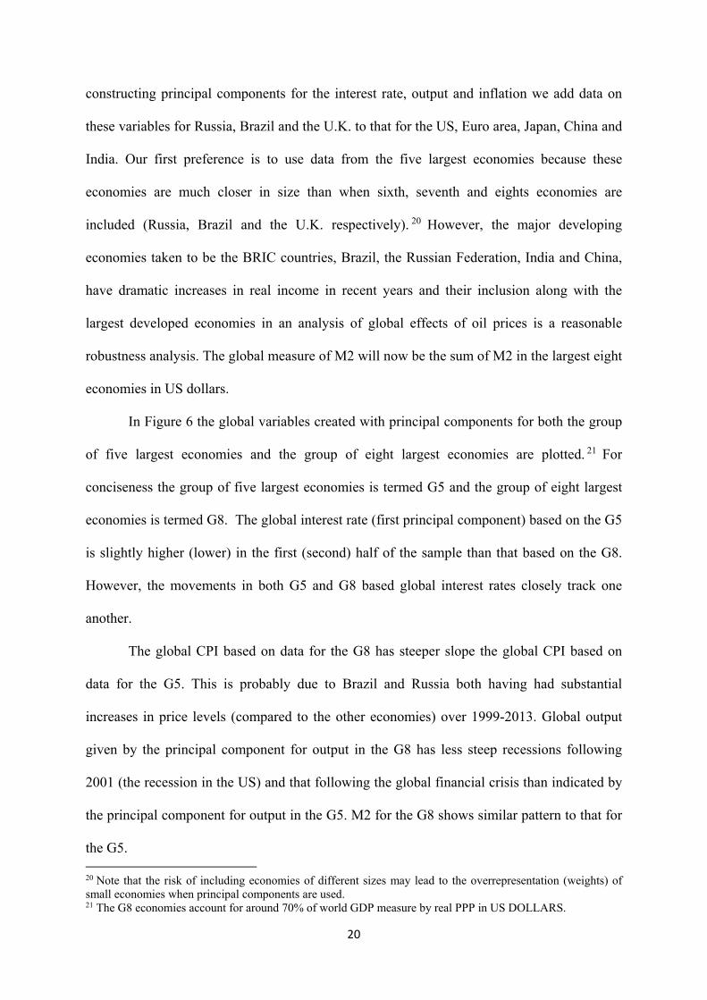
In Figure 6 the global variables created with principal components for both the group

of five largest economies and the group of eight largest economies are plotted. 21 For

conciseness the group of five largest economies is termed G5 and the group of eight largest

economies is termed G8. The global interest rate (first principal component) based on the G5

is slightly higher (lower) in the first (second) half of the sample than that based on the G8.

However, the movements in both G5 and G8 based global interest rates closely track one

another.

The global CPI based on data for the G8 has steeper slope the global CPI based on

data for the G5. This is probably due to Brazil and Russia both having had substantial

increases in price levels (compared to the other economies) over 1999-2013. Global output

given by the principal component for output in the G8 has less steep recessions following

2001 (the recession in the US) and that following the global financial crisis than indicated by 

the principal component for output in the G5. M2 for the G8 shows similar pattern to that for

the G5.                                                             20 Note that the risk of including economies of different sizes may lead to the overrepresentation (weights) of small economies when principal components are used. 21 The G8 economies account for around 70% of world GDP measure by real PPP in US DOLLARS.

21  

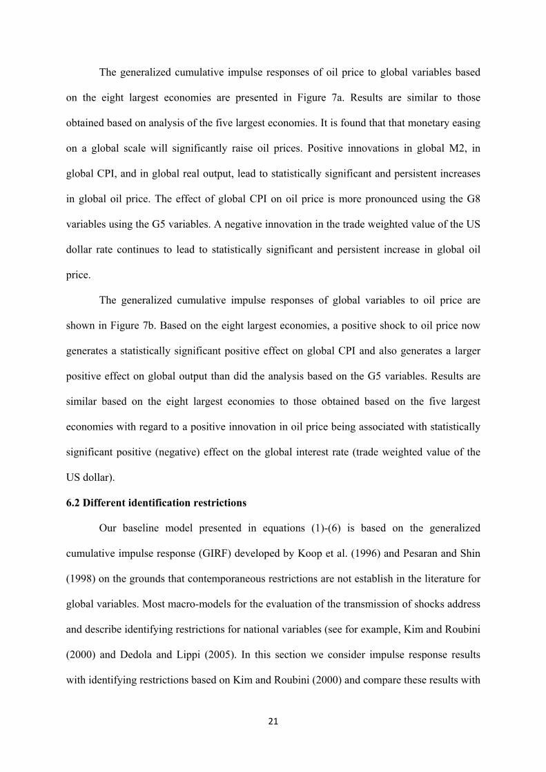
The generalized cumulative impulse responses of oil price to global variables based

on the eight largest economies are presented in Figure 7a. Results are similar to those

obtained based on analysis of the five largest economies. It is found that that monetary easing

on a global scale will significantly raise oil prices. Positive innovations in global M2, in

global CPI, and in global real output, lead to statistically significant and persistent increases

in global oil price. The effect of global CPI on oil price is more pronounced using the G8

variables using the G5 variables. A negative innovation in the trade weighted value of the US

dollar rate continues to lead to statistically significant and persistent increase in global oil

price.

The generalized cumulative impulse responses of global variables to oil price are

shown in Figure 7b. Based on the eight largest economies, a positive shock to oil price now

generates a statistically significant positive effect on global CPI and also generates a larger

positive effect on global output than did the analysis based on the G5 variables. Results are

similar based on the eight largest economies to those obtained based on the five largest

economies with regard to a positive innovation in oil price being associated with statistically

significant positive (negative) effect on the global interest rate (trade weighted value of the

US dollar).

6.2 Different identification restrictions

Our baseline model presented in equations (1)-(6) is based on the generalized

cumulative impulse response (GIRF) developed by Koop et al. (1996) and Pesaran and Shin

(1998) on the grounds that contemporaneous restrictions are not establish in the literature for

global variables. Most macro-models for the evaluation of the transmission of shocks address

and describe identifying restrictions for national variables (see for example, Kim and Roubini

(2000) and Dedola and Lippi (2005). In this section we consider impulse response results

with identifying restrictions based on Kim and Roubini (2000) and compare these results with

22  

those obtained with generalized impulse response function. In the Kim and Roubini (2000)

model, the monetary policy feedback rule does not allow monetary policy to respond within

the month to price level and output events, but allows contemporaneous response to both

monetary aggregates and oil prices.

Monetary aggregates M2 respond contemporaneously to the domestic interest rate,

CPI and real output assuming that the real demand for money depends contemporaneously on

the interest rate and real income. The CPI is influenced contemporaneously by both real

output and oil prices, while real output is assumed to be influenced by oil prices.22 Oil prices

are assumed to be contemporaneously exogenous to all variables in the model on the ground

of information delay. Given the forward looking nature of exchange rate on asset prices and

this variable’s information is available daily, the exchange rate is assumed to respond

contemporaneously to all variables in the model.

In line with this discussion of identifying restrictions based on Kim and Roubini

(2000), the matrix in equation (5) is given by:

1 0 01 0 0

0 0 1 00 0 0 1 00 0 0 0 1 0

1

∆ log ∆ log 2 ∆ log∆ log ∆ log∆log

(7)

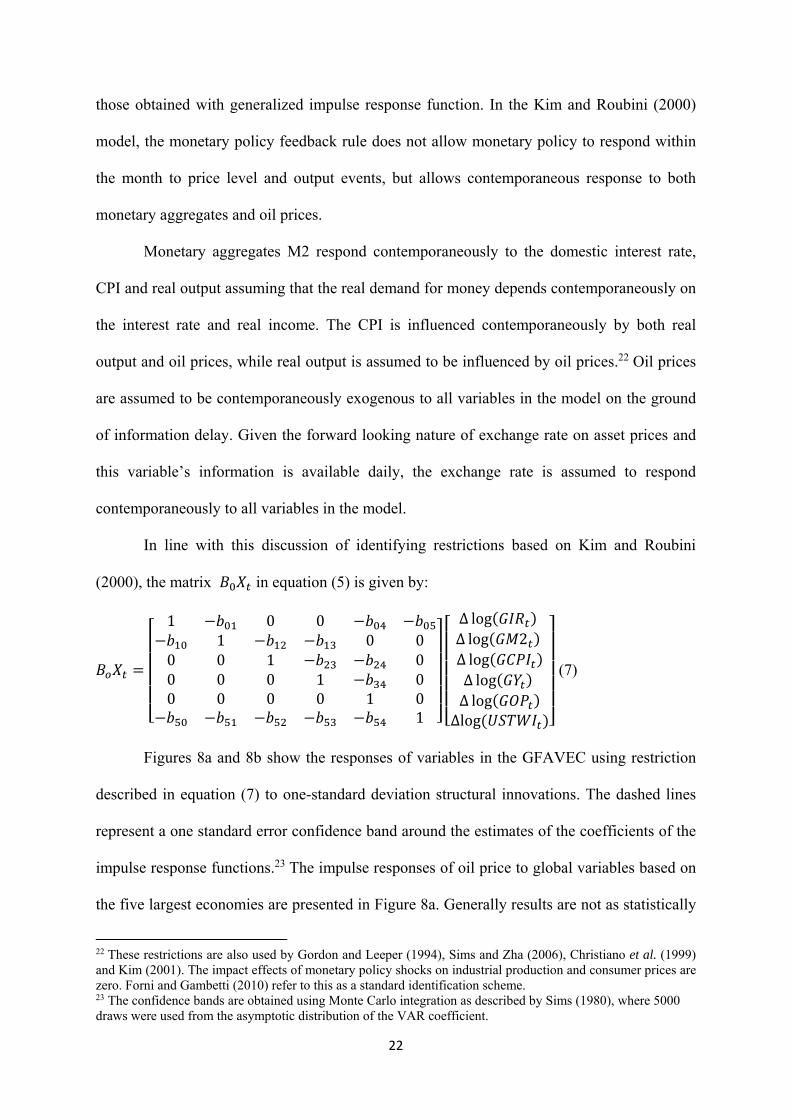
Figures 8a and 8b show the responses of variables in the GFAVEC using restriction

described in equation (7) to one-standard deviation structural innovations. The dashed lines

represent a one standard error confidence band around the estimates of the coefficients of the

impulse response functions.23 The impulse responses of oil price to global variables based on

the five largest economies are presented in Figure 8a. Generally results are not as statistically

                                                            22 These restrictions are also used by Gordon and Leeper (1994), Sims and Zha (2006), Christiano et al. (1999) and Kim (2001). The impact effects of monetary policy shocks on industrial production and consumer prices are zero. Forni and Gambetti (2010) refer to this as a standard identification scheme. 23 The confidence bands are obtained using Monte Carlo integration as described by Sims (1980), where 5000 draws were used from the asymptotic distribution of the VAR coefficient.

23  

significant as the generalized impulse response. In Figure 8a shocks to monetary easing and

CPI, and negative innovation in the trade weighted value of the US dollar do affect raise oil

prices, but the effect is smaller and statistically significant for as long as before.

The impulse responses of global variables to oil price are presented in Figure 8b.

These structural impulse responses are very similar the generalized impulse responses

reported in Figure 5. A positive innovation in oil price is associated with a statistically

significant positive effect on the global interest rate and on global real output. Positive shocks

to oil price have significant effects on global M2 and global CPI at impact only. A positive

shock in oil price leads to a significant decline in the trade weighted value of the US dollar.

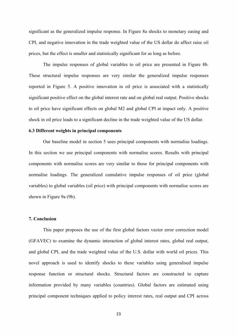
6.3 Different weights in principal components

Our baseline model in section 5 uses principal components with normalise loadings.

In this section we use principal components with normalise scores. Results with principal

components with normalise scores are very similar to those for principal components with

normalise loadings. The generalized cumulative impulse responses of oil price (global

variables) to global variables (oil price) with principal components with normalise scores are

shown in Figure 9a (9b).

7. Conclusion

This paper proposes the use of the first global factors vector error correction model

(GFAVEC) to examine the dynamic interaction of global interest rates, global real output,

and global CPI, and the trade weighted value of the U.S. dollar with world oil prices. This

novel approach is used to identify shocks to these variables using generalised impulse

response function or structural shocks. Structural factors are constructed to capture

information provided by many variables (countries). Global factors are estimated using

principal component techniques applied to policy interest rates, real output and CPI  across

24  

countries. The collective stance of monetary policy actions by major central banks is caught

by the level of global interest rates. A global factor is also estimated for the global price of oil

from the various leading oil price indices.

In line with the quantity theory at country economy level, global money, global output

and global prices are found to be cointegrated.  Granger causality is found to go from global

liquidity to oil prices and from oil prices to the global interest rate, global output and global

CPI.  Monetary tightening indicated by positive innovation in central bank discount rates

results in significant and sustained decreases in oil prices. Positive shocks to global M2, to

global CPI, and to global real output, lead to statistically significant and persistent increases

in global oil price. A negative innovation in the trade weighted value of the US dollar rate

leads to statistically significant and persistent increase in global oil price in US dollars. A rise

in oil price results in significant increases in global interest rates. A positive innovation in

(US dollar) oil price leads to a decline in the trade weighted value of the US dollar rate.

Granger causality test from economy level to global level variables shows that for the

period 1999-2013, the U.S. and China variables Granger cause the global variables, global

interest rate, global M2, global output and global CPI. The Euro area variables Granger cause

3 out of 4 global variables (global interest rate, global output and global CPI), and India and

Japan Granger cause 2 out of 4 global variables (Japan’s variables influence global M2 and

global output while India’s variables influence global output and global CPI). The results

indicate a degree of interdependence and influence between China and the global economy

that is somewhat similar to levels of interdependence between the global economy and either

the U.S. or Euro area.

25  

References Abdallah, C.S., Lastrapes, W.D., 2013. Evidence on the Relationship between Housing and Consumption in the United States: A State-Level Analysis. Journal of Money, Credit and Banking 45, 559-589. Aloui, R., Ben Aïssa, M.S., Nguyen, D.K., 2013. Conditional dependence structure between oil prices and exchange rates: A copula-GARCH approach. Journal of International Money and Finance 32 (1), 719-738. Bachmeier, L.J., Swanson, N.R., 2005. Predicting Inflation: Does The Quantity Theory Help? Economic Inquiry 43, 570-585. Barsky, R.B., Kilian, L., 2002. Do We Really Know that Oil Caused the Great Stagflation? A Monetary Alternative, in Bernanke, B.S., Rogoff, K. (Eds.), NBER Macroeconomics Annual 2001, MIT Press: Cambridge, MA, pp. 137-183. Beckmann, J, Belke, A and Czudaj, R., 2014. The importance of global shocks for national policymakers-rising challenges for sustainable monetary policies. The World Economy (forthcoming). Beirne, J., Beulen, C., Liu, G., Mirzaei, A., 2013. Global oil prices and the impact of China. China Economic Review 27, 37-51. Belke, A., Bordon, I., Hendricks, T., 2010. Global liquidity and commodity prices-a cointegrated VAR approach for OECD countries. Applied Financial Economics 20, 227-242. Belke, A., Orth, W., Setzer, R., 2010. Liquidity and the dynamic pattern of asset price adjustment: A global view. Journal of Banking and Finance 34, 1933-1945. Belviso, F., Milani, F., 2006. Structural factor-augmented VARs (SFAVARs) and the effects of monetary policy. Topics in Macroeconomics, 6-3, Article number 2. Incorporated in: B.E. Journal of Macroeconomics. Bernanke, B., Boivin, J., Eliasz, P.S., 2005. Measuring the Effects of Monetary Policy: A Factor-augmented Vector Autoregressive (FAVAR) Approach. Quarterly Journal of Economics 120, 387-422. Bernanke B.S., Gertler, M., Watson, M.W., 1997. Systematic Monetary Policy and the Effects of Oil Price Shocks. Brookings Papers on Aggregate demand 1, 91-142. Bodenstein, M., Guerrieri, L., Kilian, L., 2012. IMF Economic Review, 60(4), 470-504 Boivin, J., Giannoni, M. P., Mihov, I., 2009. Sticky Prices and Monetary Policy: Evidence from Disaggregated US Data. American Economic Review 99, 350–84. Boivin, J., Ng, S., 2006. Are more data always better for factor analysis? Journal of Econometrics, 132 (1), 169-194.

26  

Browne, F., Cronin, D., 2010. Commodity Prices, Money and Inflation. Journal of Economics and Business 62, 331-345. Cagliarini, A., McKibbin, W., 2010. Global Relative Price Shocks: The Role of Macroeconomic Policies, in: Fry, R., Jones, C., and C. Kent (eds.), Inflation in an Era of Relative Price Shocks, Sydney, 305-333. Canova, F., 2005. The transmission of US shocks to Latin America. Journal of Applied Econometrics 20, 229–251. Christiano, L.J., Eichenbaum, M., Evans, C., 1999. Monetary policy shocks: What have we learned and to what end? In: Taylor, J.B., Woodford, M. (Eds.), Handbook of Macroeconomics, Vol. 1A. North-Holland, Amsterdam, 65–148. Ciccarelli, M., Mojon, B., 2009. Global Inflation. Review of Economics and Statistics 92, 524–535. Cologni, A., Manera, M., 2008. Oil prices, inflation and interest rates in a structural cointegrated VAR model for the G-7 countries. Energy Economics 38, 856–888. Cunado, J., Perez de Garcia, F., 2005. Oil prices, economic activity and inflation: evidence for some Asian countries. The Quarterly Review of Economics and Finance 45 (1), 65–83. Dave, C., Dressler, S. J., Zhang, L., 2013. The Bank Lending Channel: A FAVAR Analysis. Journal of Money, Credit and Banking 45, 1705-1720. Dedola, L., Lippi, F., 2005. The monetary transmission mechanism: Evidence from the industries of five OECD countries, European Economic Review 49, 1543-1569.

Dees, S., di Mauro, F., Pesaran, M.H., Smith, L.V., 2007, Exploring the international linkages of the euro area: a global VAR analysis. Journal of Applied Econometrics 22, 1-38. Engle, R.F., Granger, C.W.J., 1987. Cointegration and Error-Correction: Representation, Estimation, and Testing. Econometrica 55, 251-276. Forni, M., Gambetti, L., 2010. The dynamic effects of monetary policy: A structural factor model approach. Journal of Monetary Economics, 57, 203-216. Forni, M., Hallin, M., Lippi, M., Reichlin, L., 2000. The Generalized Dynamic Factor Model: Identification and Estimation. The Review of Economics and Statistics 82, 540–554. Frankel J.A., 1986. Expectations and Commodity Price Dynamics: The Overshooting Model. American Journal of Agricultural Economics 68, 344-348. Frankel, J.A., Rose, K.A., 2010. Determinants of Agricultural and Mineral Commodity Prices, in: Fry, R., Jones, C., and C. Kent (eds), Inflation in an Era of Relative Price Shocks, Sydney, 9-51.

27  

Gilchrist, S., Yankov, V., Zakrajšek, E., 2009. Credit market shocks and economic fluctuations: Evidence from corporate bond and stock markets. Journal of Monetary Economics 56 (4), 471-493. Gordon, D.B., Leeper, E.M., 1994. The Dynamic Impacts of Monetary Policy: An Exercise in Tentative Identification. Journal of Political Economy 102, 1228-47. Hamilton, J.D., 1983. Oil and the macroeconomy since World War II. Journal of Political Economy 91, 228–248. Hamilton, J.D., 1996. This is What Happened to the Oil Price-Macroeconomy Relationship. Journal of Monetary Economics, 38, 215-20. Hamilton, J.D., 2009. Causes and Consequences of the Oil Shock of 2007-08. Brookings Papers on Economic Activity 1, Spring, 215-261. Hamilton, J.D., 2013. Historical Oil Shocks, in: Parker, R.E., Whaples, R.M., (eds.), The Routledge Handbook of Major Events in Economic History. New York: Routledge Taylor and Francis Group, 239-265. Hammoudeh, S., Nguyen, D.K., Sousa, R.M., 2015. US monetary policy and sectoral commodity prices, Journal of International Money and Finance, http://dx.doi.org/10.1016/j.jimonfin.2015.06.003 Jimenez-Rodriguez, R., Sanchez, M., 2005. Oil price shocks and real GDP growth: empirical evidence for some OECD countries. Applied Economics 37 (2), 201–228. Juvenal, L., Petrella, I., 2014. Speculation in the Oil Market. Journal of Applied Econometrics. DOI: 10.1002/jae.2388 Kilian, L., Hicks, B., 2013. Did Unexpectedly Strong Economic Growth Cause the Oil Price Shock of 2003-2008? Journal of Forecasting 32, 385-394. Kilian, L., Lee, T.K., 2014. Quantifying the Speculative Component in the Real Price of Oil: The Role of Global Oil Inventories. Journal of International Money and Finance 42, 71-87. Kilian, L., Murphy, D.P., 2014. The Role of Inventories and Speculative Trading in the Global Market for Crude Oil. Journal of Applied Econometrics, 29(3), 454-478. Kim, H., Taylor, M. P., 2012. Large Datasets, Factor-augmented and Factor-only Vector Autoregressive Models, and the Economic Consequences of Mrs Thatcher. Economica, 79, 378-410. Kim, S., 2001. International transmission of US Monetary policy shocks: evidence from VARs. Journal of Monetary Economics 48, 339–372. Kim, S., Roubini, N., 2000. Exchange rate anomalies in the industrial countries: a solution with a structural VAR approach. Journal of Monetary Economics 45, 561–586.

28  

Koop, G., Korobilis, D., 2009. Bayesian multivariate time series methods for empirical macroeconomics. Foundations and Trends in Econometrics, 3 (4), 267-358. Koop, G., Pesaran, M.H., Potter, S.M., 1996. Impulse response analysis in nonlinear multivariate models. Journal of Econometrics 74, 119–147. Laganà, G., (2009). A structural factor-augmented vector error correction (SFAVEC) model approach: An application to the UK. Applied Economics Letters, 16 (17), 1751-1756. Le Bihan, H., Matheron, J., 2012. Price Stickiness and Sectoral Inflation Persistence: Additional Evidence. Journal of Money, Credit and Banking 15, 1427-1442. Lee, K., Ni, S., Ratti, R.A., 1995. Oil shocks and the macroeconomy: the role of price variability. Energy Journal 16 (4), 39–56. Lombardi, M. J., Osbat, C., Schnatz, B., 2012. Global commodity cycles and linkages: a FAVAR approach. Empirical Economics 43, 651-670. Mallick, S.K., Sousa, R.M., 2013. Commodity Prices, Inflationary Pressures, and Monetary Policy: Evidence from BRICS Economies. Open Economies Review 24 (4), 677-694.

Mumtaz, H., Surico, P., 2009. The Transmission of International Shocks: A Factor-Augmented VAR Approach. Journal of Money, Credit and Banking 41, 71-100.

Mumtaz, H., Surico, P., 2012. Evolving International Inflation Dynamics: World and Country-Specific Factors. Journal of the European Economic Association 2012, 716–734.

Pesaran, M.H., Schuermann, T., Weiner, S.M., 2004. Modelling Regional Interdependencies Using a Global Error Correcting Macroeconometric Model, Journal of Business and Economic Statistics, 22, 2, 129–62.

Pesaran, M.H., Shin, Y., 1998. Generalized Impulse Response Analysis in Linear Multivariate Models. Economics Letters 58, 17–29.

Ratti, R.A., Vespignani, J.L., 2013. Why are crude oil prices high when global activity is weak? Economics Letters 121, 133–136. Shin, H. S., 2014. Financial stability risks: old and new. Bank for International Settlements, Management Speech at the Brookings Institution, Washington DC, 4 December 2014. Sims, C.A., 1980. Macroeconomics and Reality. Econometrica 48, 1-48. Sims, C.A., Zha, T., 1995. Does monetary policy generate recessions?: Using less aggregate price data to identify monetary policy. Working paper, Yale University, CT. Sims, C., 2002. The Role of Models and Probabilities in the Monetary Policy Process. mimeo, Princeton University. Sims, C.A., Zha, T., 2006. Does Monetary Policy Generate Recessions?, Macroeconomic Dynamics 10, 231-272.

29  

Stock, J., Watson, M., 1998. Diffusion Indexes. NBER Working Paper No. 6702. Stock, J.H., Watson, M.W., 2002. Forecasting using principal components from a large number of predictors. Journal of the American Statistical Association 97, 1167–1179. Stock, J., Watson, M., 2005. Macroeconomic Forecasting Using Diffusion Indexes. Journal of Business and Economic Statistics 20, 147–62. Swanson, N.R., 1998. Money and output viewed through a rolling window. Journal of Monetary Economics 41, 455-474. Thornton, D.L., 2014. Monetary policy: Why money matters (and interest rates don't). Journal of Macroeconomics 40, 202-213. Valadkhani, A., 2014. Dynamic effects of rising oil prices on consumer energy prices in Canada and the United States: Evidence from the last half a century, Energy Economics 45, 33-44.

30  

Table 1: Correlation between the logs of country-specific and global variables

Country M2 in US dollars Interest rate Real output CPI

Euro area 0.96 0.76 0.65 0.96

US 0.99 0.54 0.88 0.95

China 0.99 0.76 0.63 0.86

Japan 0.93 0.77 0.71 0.82

India 0.97 0.29 0.88 0.89 Table 2: Granger causality tests for global variables 1999:1-2013:12 (log-level)

Null hypothesis: variable x does not Granger cause variable y

Alternative hypothesis: variable x Granger cause variable y

Granger test/Lags 1 3 6 12 24

GOP does not Granger cause GIR 2.78*** 2.17* 3.57*** 2.51*** 1.79**

GIR does not Granger cause GOP 0.70 0.87 0.69 1.34 1.56*

GOP does not Granger cause GM2 0.01 0.39 1.85* 1.22 0.79

GM2 does not Granger GOP 6.83*** 3.46*** 2.18** 1.82* 0.94

GOP does not Granger cause GY 1.51 8.33*** 5.99*** 3.20*** 2.13***

GY does not Granger cause GOP 0.23 1.98 1.06 1.50 0.81

GOP does not Granger cause GCPI 1.99 2.14* 1.40 2.45*** 1.85**

GCPI does not Granger cause GOP 0.66 2.13* 1.32 1.53 1.12 Notes: ***, **,* Indicates rejection of the null hypothesis at 1, 5 and 10% level of significance, respectively.

Table 3a: Granger causality tests for GIR vs. country-specific IR 1999:1-2013:12 (log-level)

Null hypothesis: variable x does not Granger cause variable y

Alternative hypothesis: variable x Granger cause variable y

Granger test/Lags 1 3 6 12 24

USIR does not Granger cause GIR 12.7*** 7.78*** 5.54*** 2.91*** 1.42

GIR does not Granger cause USIR 33.02*** 4.82*** 2.55*** 1.21 0.97

EAIR does not Granger cause GIR 4.27*** 5.69*** 2.79*** 1.10 0.97

GIR does not Granger cause EAIR 6.00*** 2.39* 4.47 1.37 1.81***

CHIR does not Granger cause GIR 14.23*** 9.24*** 3.80*** 3.24*** 2.26***

GIR does not Granger cause CHIR 7.17*** 4.81*** 3.12*** 3.24*** 1.79***

INIR does not Granger cause GIR 0.39 0.44 0.52 0.35 0.48

GIR does not Granger cause INIR 0.15 0.33 0.18 0.30 0.36

JAPIR does not Granger cause GIR 0.84 0.57 0.89 2.36*** 1.57*

GIR does not Granger cause JAPIR 1.99 3.13*** 1.56 1.49 1.25 Notes: ***, **,* Indicates rejection of the null hypothesis at 1, 5 and 10% level of significance, respectively.

31  

Table 3b: Granger causality tests for GM2 vs. country-specific M2 1999:1-2013:12 (log-level)

Null hypothesis: variable x does not Granger cause variable y

Alternative hypothesis: variable x Granger cause variable y

Granger test/Lags 1 3 6 12 24

USM2 does not Granger cause GM2 7.98*** 3.58*** 2.32** 2.25** 1.92**

GM2 does not Granger cause USM2 0.06 1.31 0.63 0.62 0.85

EAM2 does not Granger cause GM2 0.34 1.11 1.23 0.90 0.95

GM2 does not Granger cause EAM2 0.00 1.47 1.13 1.20 1.30

CHM2 does not Granger cause GM2 7.41*** 2.42* 1.17 1.17 1.44

GM2 does not Granger cause CHM2 0.97 0.49 0.82 0.81 1.10

INM2 does not Granger cause GM2 3.46* 1.10 1.63 1.30 0.81

GM2 does not Granger cause INM2 0.75 1.83 1.07 1.36 1.17

JAPM2 does not Granger cause GM2 5.73*** 5.20*** 2.94*** 2.07** 1.10

GM2 does not Granger cause JAPM2 5.17*** 4.59*** 2.15* 1.63* 1.48* Notes: ***, **,* Indicates rejection of the null hypothesis at 1, 5 and 10% level of significance, respectively.

Table 3c: Granger causality tests for GY vs. country-specific Y1999:1-2013:12 (log-level)

Null hypothesis: variable x does not Granger cause variable y

Alternative hypothesis: variable x Granger cause variable y

Granger test/Lags 1 3 6 12 24

USY does not Granger cause GY 0.29 2.02 5.39*** 3.55*** 2.27***

GY does not Granger cause USY 0.84 6.34*** 3.07*** 2.17** 1.51*

EAY does not Granger cause GY 1.87 2.88** 5.40*** 3.57*** 2.28***

GY does not Granger cause EAY 1.58 4.05*** 1.34 2.07** 1.44

CHY does not Granger cause GY 0.01 4.66*** 1.95* 1.28 1.40

GY does not Granger cause CHY 21.66*** 1.37 0.99 1.51 1.57*

INYdoes not Granger cause GY 0.02 4.32*** 2.21* 1.48 1.26

GY does not Granger cause INY 0.18 2.47* 1.68 1.11 1.32

JAPY does not Granger cause GY 2.29 3.24*** 1.14 0.96 0.70

GY does not Granger cause JAPY 0.21 2.95*** 2.52** 1.97** 1.62* Notes: ***, **,* Indicates rejection of the null hypothesis at 1, 5 and 10% level of significance, respectively.

32  

Table 3d: Granger causality tests for GCPI vs. country-specific CPI 1999:1-2013:12 (log-level)

Null hypothesis: variable x does not Granger cause variable y

Alternative hypothesis: variable x Granger cause variable y

Granger test/Lags 1 3 6 12 24

USCPI does not Granger cause GCPI 3.06** 1.37 1.97 2.21** 1.00

GCPI does not Granger cause USCPI 1.74 1.70 0.68 1.26 1.20

EACPI does not Granger cause GCPI 2.94* 1.89 4.09*** 2.25*** 1.39*

GCPI does not Granger cause EACPI 3.33* 1.04 1.79 2.28*** 2.24

CHCPI does not Granger cause GCPI 1.24 1.00 5.29*** 6.75*** 1.95**

GCPI does not Granger cause CHCPI 4.43** 12.60*** 13.46*** 4.28*** 1.83**

INCPIdoes not Granger cause GCPI 3.56* 1.23 5.23*** 4.13*** 1.23

GCPI does not Granger cause INCPI 0.13 1.37 0.86 1.45 0.24

JAPCPI does not Granger cause GCPI 1.42 0.60 1.22 0.91 1.07

GCPI does not Granger cause JAPCPI 2.37 2.46* 1.65 1.80* 1.35 Notes: ***, **,* Indicates rejection of the null hypothesis at 1, 5 and 10% level of significance, respectively. Table 4: Test for unit roots 1999:1-2013:12: Data in level

Null hypothesis for ADF test: the variable has a unit root

Alternative hypothesis for ADF test: the variable has not a unit root

Null hypothesis for KPSS test: variable is stationary

Alternative hypothesis for KPSS test: variable is not stationary

Level ADF KPSS First difference ADF KPSS

log (GM2t) 0.92 1.61*** ∆log (G3M2t) -12.90*** 0.24

log (GCPIt) -1.92 1.52*** ∆log (GCPIt) 1.00*** 0.73

log (GIPt) -2.94* 0.77*** ∆log (GIPt) -4.56*** 0.09

log (GOPt) -2.51 1.51*** ∆log (GOPt) -10.01*** 0.11

log (USTWIt) -0.99 1.41*** ∆log (USTWIt) -9.22*** 0.09 Notes: The first difference of the series is indicated by ∆.The lag selection criteria for the ADF is based on Schwarz information Criteria (SIC) and for the KPSS is the Newey-West Bandwidth. ***, **,* Indicates rejection of the null hypothesis at 1, 5 and 10% level of significance, respectively.

33  

Table 5: Cointegration test: logs of global CPI (GCPI), money (G3 M2 and BRIC M2) and global output (GY). a) Cointegration test with different specifications

Endogenous variables: log(global CPIt), log(global M2t), log(global real outputt)

Test Type None trend and Intercept Linear trend and Intercept

Trace 1 1

Max-Eig 1 1 Notes: *Critical values based on MacKinnon-Haug-Michelis (1999). **Selected (0.05 level*) Number of Cointegrating Relations by Model.

b) Unrestricted cointegration rank test (trace) Null hypothesis: the number of cointegrating vectors is less than or equal to r

Alternative hypothesis: there are more than r cointegrating vectors

Hypothesized Eigenvalue

Trace statistic

0.05 Critical value

Prob.** Null Alternative

r=0 r≥1 0.19 45.5 29.79 0.00

r≤1 r≥2 0.05 9.94 15.49 0.28

r≤2 r≥3 0.00 0.24 3.94 0.62 **MacKinnon-Haug-Michelis (1999) p-values

c) Unrestricted cointegration rank test (maximum eigenvalue) Null hypothesis: the number of cointegrating vectors is r

Alternative hypothesis: there are (r+1) cointegrating vectors

Hypothesized Eigenvalue

Max-eigenvalue stat.

0.05 Critical value

Prob.** Null Alternative

r=0 r=1 0.22 60.83 42.9 0.00

r=1 r=2 0.07 20.9 25.88 0.18

r=2 r=3 0.04 7.94 12.52 0.25 **MacKinnon-Haug-Michelis (1999) p-values

Table 6. LR test Null hypothesis for LR test: no structural change

Alternative hypothesis for LR test: structural change

Degree of freedom

critical value with at 95%

value

Dummy variable: 2008:M9 to data end 6 12.59 5.95

Dummy variable: 2008:M9 to 2008:M12 6 12.59 39.66***

Dummy variable: 2009:M1 to data end 6 12.59 2.14 Notes: The LR test is |Σ | | | ~ , where: T is the number of observations, m is the is the number of parameters in each equation of the unrestricted system plus contains, Σ is the determinant of the residual covariance matrix, and q is the number of dummy variables times number of equations.

34  

Figure 1. a)G5 Interest rate b)Logs of G5 M2 in US dollars

c)Logs of G5 real output d)Logs of G5 CPI

Notes: Central bank discount rates, M2 monetary aggregates, consumer price indices, and industrial production indices are for each of the five largest economies (the G5). The G5 consists of the US, the Euro area, Japan, China and India. Interest rates are in percent. Log of M2 data in US dollars is shown. Logs of industrial production and the CPI are also shown. Data are monthly.

Figure 2. US dollar indexes for Brent, Dubai and WTI crude oil prices

Notes: Brent, Dubai and West Texas Intermediate crude oil prices are US dollar indices. Data are monthly.

35  

Figure 3. Scree plot (ordered eigenvalues) for global principal components

     

0.0

0.5

1.0

1.5

2.0

2.5

3.0

1 2 3 4 5

Global interest rate

0.0

0.5

1.0

1.5

2.0

2.5

3.0

1 2 3 4 5

Global outputs

0

1

2

3

4

5

1 2 3 4 5

Global CPI

0.0

0.5

1.0

1.5

2.0

2.5

3.0

1 2 3

Global oil prices

36  

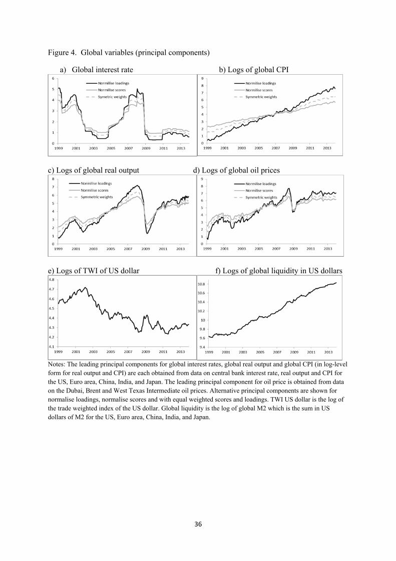
Figure 4. Global variables (principal components)

a) Global interest rate b) Logs of global CPI

c) Logs of global real output d) Logs of global oil prices

e) Logs of TWI of US dollar f) Logs of global liquidity in US dollars

 Notes: The leading principal components for global interest rates, global real output and global CPI (in log-level form for real output and CPI) are each obtained from data on central bank interest rate, real output and CPI for the US, Euro area, China, India, and Japan. The leading principal component for oil price is obtained from data on the Dubai, Brent and West Texas Intermediate oil prices. Alternative principal components are shown for normalise loadings, normalise scores and with equal weighted scores and loadings. TWI US dollar is the log of the trade weighted index of the US dollar. Global liquidity is the log of global M2 which is the sum in US dollars of M2 for the US, Euro area, China, India, and Japan.

37  

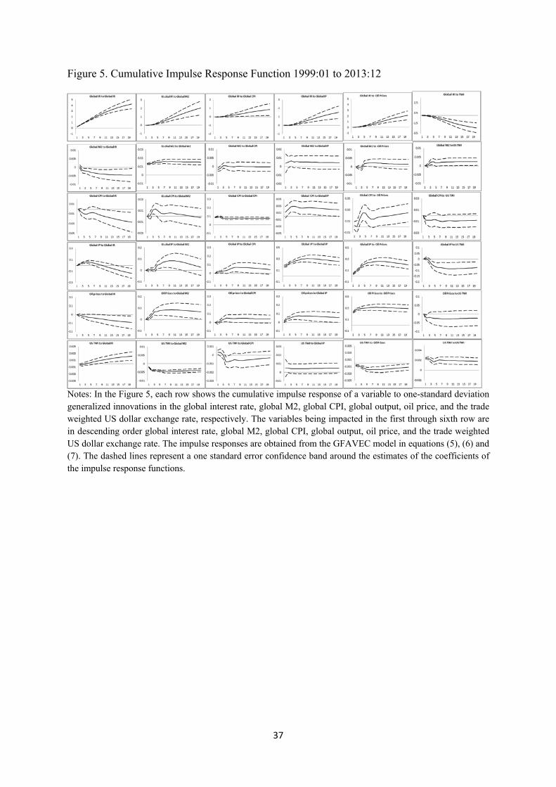
Figure 5. Cumulative Impulse Response Function 1999:01 to 2013:12

 

 

 

 Notes: In the Figure 5, each row shows the cumulative impulse response of a variable to one-standard deviation generalized innovations in the global interest rate, global M2, global CPI, global output, oil price, and the trade weighted US dollar exchange rate, respectively. The variables being impacted in the first through sixth row are in descending order global interest rate, global M2, global CPI, global output, oil price, and the trade weighted US dollar exchange rate. The impulse responses are obtained from the GFAVEC model in equations (5), (6) and (7). The dashed lines represent a one standard error confidence band around the estimates of the coefficients of the impulse response functions.

38  

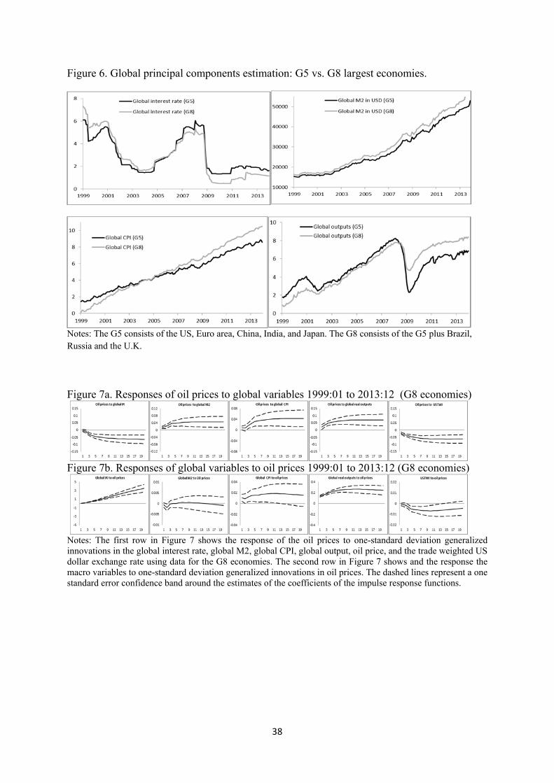
Figure 6. Global principal components estimation: G5 vs. G8 largest economies.

 

Notes: The G5 consists of the US, Euro area, China, India, and Japan. The G8 consists of the G5 plus Brazil, Russia and the U.K.

Figure 7a. Responses of oil prices to global variables 1999:01 to 2013:12 (G8 economies)

Figure 7b. Responses of global variables to oil prices 1999:01 to 2013:12 (G8 economies)

Notes: The first row in Figure 7 shows the response of the oil prices to one-standard deviation generalized innovations in the global interest rate, global M2, global CPI, global output, oil price, and the trade weighted US dollar exchange rate using data for the G8 economies. The second row in Figure 7 shows and the response the macro variables to one-standard deviation generalized innovations in oil prices. The dashed lines represent a one standard error confidence band around the estimates of the coefficients of the impulse response functions.

39  

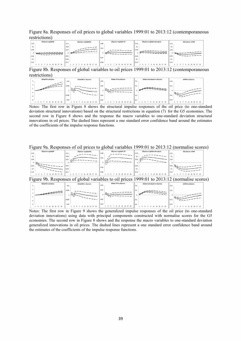
Figure 8a. Responses of oil prices to global variables 1999:01 to 2013:12 (contemporaneous restrictions)

Figure 8b. Responses of global variables to oil prices 1999:01 to 2013:12 (contemporaneous restrictions)

Notes: The first row in Figure 8 shows the structural impulse responses of the oil price (to one-standard deviation structural innovations) based on the structural restrictions in equation (7)  for the G5 economies. The second row in Figure 8 shows and the response the macro variables to one-standard deviation structural innovations in oil prices. The dashed lines represent a one standard error confidence band around the estimates of the coefficients of the impulse response functions. Figure 9a. Responses of oil prices to global variables 1999:01 to 2013:12 (normalise scores)

Figure 9b. Responses of global variables to oil prices 1999:01 to 2013:12 (normalise scores)

Notes: The first row in Figure 9 shows the generalized impulse responses of the oil price (to one-standard deviation innovations) using data with principal components constructed with normalise scores for the G5 economies. The second row in Figure 8 shows and the response the macro variables to one-standard deviation generalized innovations in oil prices. The dashed lines represent a one standard error confidence band around the estimates of the coefficients of the impulse response functions.  

 

 

 

TASMANIAN SCHOOL OF BUSINESS AND ECONOMICS WORKING PAPER SERIES

2014-09 VAR Modelling in the Presence of China’s Rise: An Application to the Taiwanese Economy. Mardi Dun-gey, Tugrul Vehbi and Charlton Martin

2014-08 How Many Stocks are Enough for Diversifying Canadian Institutional Portfolios? Vitali Alexeev and Fran-cis Tapon

2014-07 Forecasting with EC-VARMA Models, George Athanasopoulos, Don Poskitt, Farshid Vahid, Wenying Yao

2014-06 Canadian Monetary Policy Analysis using a Structural VARMA Model, Mala Raghavan, George Athana-sopoulos, Param Silvapulle

2014-05 The sectorial impact of commodity price shocks in Australia, S. Knop and Joaquin Vespignani

2014-04 Should ASEAN-5 monetary policymakers act pre-emptively against stock market bubbles? Mala Raghavan and Mardi Dungey

2014-03 Mortgage Choice Determinants: The Role of Risk and Bank Regulation, Mardi Dungey, Firmin Doko Tchatoka, Graeme Wells, Maria B. Yanotti

2014-02 Concurrent momentum and contrarian strategies in the Australian stock market, Minh Phuong Doan, Vi-tali Alexeev, Robert Brooks

2014-01 A Review of the Australian Mortgage Market, Maria B. Yanotti

2014-10 Contagion and Banking Crisis - International Evidence for 2007-2009 , Mardi Dungey and Dinesh Gaju-rel

2014-11 The impact of post‐IPO changes in corporate governance mechanisms on firm performance: evidence from young Australian firms, Biplob Chowdhury, Mardi Dungey and Thu Phuong Pham

2014-12 Identifying Periods of Financial Stress in Asian Currencies: The Role of High Frequency Financial Market Data, Mardi Dungey, Marius Matei and Sirimon Treepongkaruna

2014-13 OPEC and non‐OPEC oil production and the global economy, Ronald Ratti and Joaquin Vespignani

2014-14 VAR(MA), What is it Good For? More Bad News for Reduced‐form Estimation and Inference, Wenying Yao, Timothy Kam and Farshid Vahid