Theoretical Computer Science 412 (2011) 7009–7017

Contents lists available at SciVerse ScienceDirect

Theoretical Computer Science

journal homepage: www.elsevier.com/locate/tcs

On computing the minimum 3-path vertex cover and dissociationnumber of graphs

František Kardoš a, Ján Katrenič b,∗, Ingo Schiermeyer ca Institute of Mathematics, P.J. Šafárik University, Košice, Slovakiab Institute of Computer Science, P.J. Šafárik University, Košice, Slovakiac Institut für Diskrete Mathematik und Algebra, TU-Freiberg, Germany

a r t i c l e i n f o

Article history:Received 18 December 2010Received in revised form 6 August 2011Accepted 7 September 2011Communicated by J. Kratochvil

Keywords:Path vertex coverDissociation numberApproximation

a b s t r a c t

The dissociation number of a graph G is the number of vertices in a maximum size inducedsubgraph of G with vertex degree at most 1. A k-path vertex cover of a graph G is a subsetS of vertices of G such that every path of order k in G contains at least one vertex fromS. The minimum 3-path vertex cover is a dual problem to the dissociation number. Forthis problem, we present an exact algorithm with a running time of O∗(1.5171n) on agraph with n vertices. We also provide a polynomial time randomized approximationalgorithm with an expected approximation ratio of 23

11 for the minimum 3-path vertexcover.

© 2011 Elsevier B.V. All rights reserved.

1. Introduction and motivation

In this paper, we consider only finite non-oriented graphs without loops ormultiple edges. A subset of vertices in a graphG is called dissociation if it induces a subgraph with maximum degree 1. The number of vertices in a maximum cardinalitydissociation set inG is called the dissociation number ofG, denoted by diss(G). The problemof computing diss(G) (dissociationnumber problem) has been introduced by Yannakakis [19], who also proved it to beNP-hard in the class of bipartite or planargraphs. Boliac et al. [2] proved that the problem remains NP-hard even in C4-free bipartite graphswith vertex degree atmost3. The dissociation number problem can be solved polynomially, e.g. for trees [16]. Polynomially solvable classes of graphsfor the dissociation number problem were also studied in [1–4,13,15]. Some combinatorial bounds on the value of diss(G)are also presented in [3,10].

Recently, Brešar et al. [3] introduced a more general concept to the dissociation number defined as follows. Let G be agraph and let k be a positive integer. A subset of vertices S ⊆ V (G) is called a k-path vertex cover if every path of orderk in G contains at least one vertex from S. Let ψk(G) be the minimum cardinality of a k-path vertex cover in G. Clearly,ψ3(G) = |V (G)|− diss(G). Denote by k-PVCP the problem to compute a k-path vertex cover of sizeψk(G). This optimizationproblem was first posed in [14].

In [3], it was proved that for any approximation rate r ≥ 1 one can transform a polynomial time r-approxima-tion for the k-PVCP to a polynomial time r-approximation algorithm for the vertex cover problem. Using the resultof [7], this implies that for every k ≥ 2 the k-PVCP is NP-hard to approximate within a factor of 1.3606, unlessP = NP .

∗ Corresponding author. Tel.: +421 904393104.E-mail address: jan.katrenic@upjs.sk (J. Katrenič).

0304-3975/$ – see front matter© 2011 Elsevier B.V. All rights reserved.doi:10.1016/j.tcs.2011.09.009

7010 F. Kardoš et al. / Theoretical Computer Science 412 (2011) 7009–7017

A well-known 2-approximation algorithm for 2-PVCP which repeatedly puts vertices of an edge into the constructedvertex cover and removes them from the graph, was discovered independently by F. Gavril and M. Yannakakis (cf. [6]).Whether there exists an r-approximation algorithm with a factor constant r < 2 is one of the major open problems forapproximation algorithms. For the k-PVCP, one can construct a k-approximation algorithm by systematically removingany path on k vertices [3]. However, to get a deterministic polynomial time approximation with a smaller constantapproximation seems to be difficult.

In this paper, we investigate on the 3-PVCP. In the first section, we provide a polynomial time randomized approximationalgorithmwith an expected approximation ratio of 23

11 , for the 3-PVCP. In the second section, we present an exact algorithmwith a running time of O∗(1.5171n) on a graph with n vertices. Throughout the paper, the notation O∗(f (n)) suppressesfactors that are polynomial in n.

2. An approximation for the minimum 3-path vertex cover

In this section, we focus on the 3-PVCP and provide a randomized approximation algorithm with an expected ratio of2+

111 . First, recall the result of [3] which is a consequence of Lovász’s decomposition [12] of a graph with maximum degree

∆ into subgraphs of maximum degree 1.

Lemma 2.1 ([3]). Let G be a graph of maximum degree∆. Then

ψ3(G) ≤⌈∆−12 ⌉

⌈∆+12 ⌉

|V (G)|.

Moreover, such a decomposition can be computed in running time O(|E(G)|∆(G)).

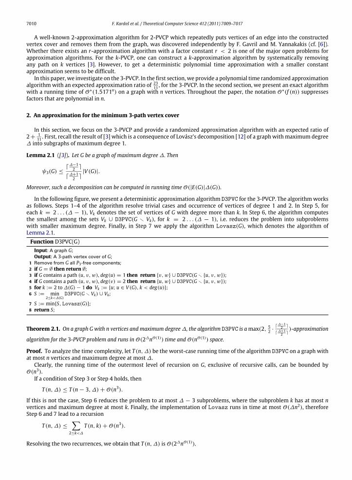
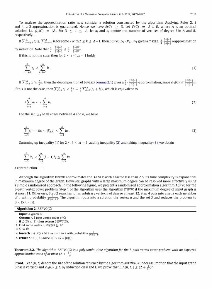
In the following figure, we present a deterministic approximation algorithm D3PVC for the 3-PVCP. The algorithmworksas follows. Steps 1–4 of the algorithm resolve trivial cases and occurrence of vertices of degree 1 and 2. In Step 5, foreach k = 2 . . . (∆ − 1), Vk denotes the set of vertices of G with degree more than k. In Step 6, the algorithm computesthe smallest among the sets Vk ∪ D3PVC(G r Vk), for k = 2 . . . (∆ − 1), i.e. reduces the problem into subproblemswith smaller maximum degree. Finally, in Step 7 we apply the algorithm Lovasz(G), which denotes the algorithm ofLemma 2.1.Function D3PVC(G)Input: A graph G;Output: A 3-path vertex cover of G;

1 Remove from G all P3-free components;2 if G = ∅ then return ∅;3 if G contains a path (u, v, w), deg(u) = 1 then return {v,w} ∪ D3PVC(G r {u, v, w});4 if G contains a path (u, v, w), deg(v) = 2 then return {u, w} ∪ D3PVC(G r {u, v, w});5 for k := 2 to∆(G)− 1 do Vk := {u; u ∈ V (G), k < deg(u)};6 S := min

2≤k<∆(G)D3PVC(G r Vk) ∪ Vk;

7 S := min{S, Lovasz(G)};8 return S;

Theorem 2.1. On a graph G with n vertices and maximum degree∆, the algorithm D3PVC is amax(2, 52 ·

⌈∆−12 ⌉

⌈∆+12 ⌉)-approximation

algorithm for the 3-PVCP problem and runs in O(2∆nO(1)) time and O(nO(1)) space.

Proof. To analyze the time complexity, let T (n,∆) be the worst-case running time of the algorithm D3PVC on a graph withat most n vertices and maximum degree at most∆.

Clearly, the running time of the outermost level of recursion on G, exclusive of recursive calls, can be bounded byO(n3).

If a condition of Step 3 or Step 4 holds, then

T (n,∆) ≤ T (n − 3,∆)+ O(n3).

If this is not the case, Step 6 reduces the problem to at most ∆ − 3 subproblems, where the subproblem k has at most nvertices and maximum degree at most k. Finally, the implementation of Lovasz runs in time at most O(∆n2), thereforeStep 6 and 7 lead to a recursion

T (n,∆) ≤

−2≤k<∆

T (n, k)+ O(n3).

Resolving the two recurrences, we obtain that T (n,∆) is O(2∆nO(1)).

F. Kardoš et al. / Theoretical Computer Science 412 (2011) 7009–7017 7011

To analyze the approximation ratio now consider a solution constructed by the algorithm. Applying Rules 2, 3and 4, a 2-approximation is guaranteed. Hence we have δ(G) ≥ 3. Let V (G) = A ∪ B, where A is an optimalsolution, i.e. ψ3(G) = |A|. For 3 ≤ i ≤ ∆, let ai and bi denote the number of vertices of degree i in A and B,respectively.

If∑∆

i=k+1 ai ≥∑∆

i=k+1 bi for some kwith 2 ≤ k ≤ ∆−1, thenD3PVC(GkrVk)∪Vk gives amax(2, 52 ·

⌈k−12 ⌉

⌈k+12 ⌉)-approximation

by induction. Note that 52 ·

⌈k−12 ⌉

⌈k+12 ⌉

≤52 ·

⌈∆−12 ⌉

⌈∆+12 ⌉.

If this is not the case, then for 2 ≤ k ≤ ∆− 1 holds

∆−i=k+1

ai <∆−

i=k+1

bi. (1)

If∑∆

i=3 ai ≥25n, then the decomposition of Lovász (Lemma 2.1) gives a 5

2 ·⌈∆−12 ⌉

⌈∆+12 ⌉

-approximation, sinceψ3(G) ≤⌈∆−12 ⌉

⌈∆+12 ⌉

n.

If this is not the case, then∑∆

i=3 ai <25n =

25

∑∆

i=3(ai + bi),which is equivalent to

3∆−i=3

ai < 2∆−i=3

bi. (2)

For the set EA,B of all edges between A and B, we have

∆−i=3

(i − 1)bi ≤ |EA,B| ≤

∆−i=3

iai. (3)

Summing up inequality (1) for 2 ≤ k ≤ ∆− 1, adding inequality (2) and taking inequality (3), we obtain

∆−i=3

iai <∆−i=3

(i − 1)bi ≤

∆−i=3

iai,

a contradiction. �

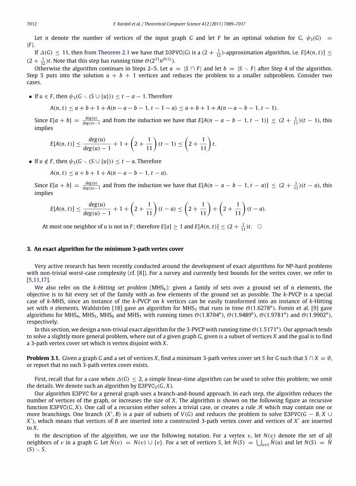
Although the algorithm D3PVC approximates the 3-PVCP with a factor less than 2.5, its time complexity is exponentialin maximum degree of the graph. However, graphs with a large maximum degree can be resolved more effectively usinga simple randomized approach. In the following figure, we present a randomized approximation algorithm A3PVC for the3-path vertex cover problem. Step 1 of the algorithm uses the algorithm D3PVC if the maximum degree of input graph isat most 11. Otherwise, Step 2 searches for an arbitrary vertex u of degree at least 12. Step 4 puts into a set S each neighborof u with probability 1

deg(u)+1 . The algorithm puts into a solution the vertex u and the set S and reduces the problem toG r (S ∪ {u}).

Algorithm 2: A3PVC(G)Input: A graph G;Output: A 3-path vertex cover of G;

1 if ∆(G) ≤ 11 then return D3PVC(G);2 Find some vertex u, deg(u) ≥ 12;3 S := ∅;

4 foreach v ∈ N(u) do insert v into S with probability 1|N(u)|−1 ;

5 return S ∪ {u} ∪ A3PVC(G r (S ∪ {u}));

Theorem 2.2. The algorithm A3PVC(G) is a polynomial time algorithm for the 3-path vertex cover problem with an expectedapproximation ratio of at most (2 +

111 ).

Proof. Let A(n, t) denote the size of the solution returned by the algorithm A3PVC(G) under assumption that the input graphG has n vertices and ψ3(G) ≤ t . By induction on n and t , we prove that E[A(n, t)] ≤ (2 +

111 )t .

7012 F. Kardoš et al. / Theoretical Computer Science 412 (2011) 7009–7017

Let n denote the number of vertices of the input graph G and let F be an optimal solution for G, ψ3(G) =

|F |.If ∆(G) ≤ 11, then from Theorem 2.1 we have that D3PVC(G) is a (2 +

112 )-approximation algorithm, i.e. E[A(n, t)] ≤

(2 +112 )t . Note that this step has running time O(211nO(1)).

Otherwise the algorithm continues in Steps 2–5. Let a = |S ∩ F | and let b = |S r F | after Step 4 of the algorithm.Step 5 puts into the solution a + b + 1 vertices and reduces the problem to a smaller subproblem. Consider twocases.

• If u ∈ F , then ψ3(G r (S ∪ {u})) ≤ t − a − 1. Therefore

A(n, t) ≤ a + b + 1 + A(n − a − b − 1, t − 1 − a) ≤ a + b + 1 + A(n − a − b − 1, t − 1).

Since E[a + b] =deg(u)

deg(u)−1 and from the induction we have that E[A(n − a − b − 1, t − 1)] ≤ (2 +111 )(t − 1), this

implies

E[A(n, t)] ≤deg(u)

deg(u)− 1+ 1 +

2 +

111

(t − 1) ≤

2 +

111

t.

• If u /∈ F , then ψ3(G r (S ∪ {u})) ≤ t − a. Therefore

A(n, t) ≤ a + b + 1 + A(n − a − b − 1, t − a).

Since E[a + b] =deg(u)

deg(u)−1 and from the induction we have that E[A(n − a − b − 1, t − a)] ≤ (2 +111 )(t − a), this

implies

E[A(n, t)] ≤deg(u)

deg(u)− 1+ 1 +

2 +

111

(t − a) ≤

2 +

111

+

2 +

111

(t − a).

At most one neighbor of u is not in F ; therefore E[a] ≥ 1 and E[A(n, t)] ≤ (2 +111 )t . �

3. An exact algorithm for the minimum 3-path vertex cover

Very active research has been recently conducted around the development of exact algorithms for NP-hard problemswith non-trivial worst-case complexity (cf. [8]). For a survey and currently best bounds for the vertex cover, we refer to[5,11,17].

We also refer on the k-Hitting set problem (MHSk): given a family of sets over a ground set of n elements, theobjective is to hit every set of the family with as few elements of the ground set as possible. The k-PVCP is a specialcase of k-MHS, since an instance of the k-PVCP on k vertices can be easily transformed into an instance of k-Hittingset with n elements. Wahlström [18] gave an algorithm for MHS3 that runs in time O(1.6278n). Fomin et al. [9] gavealgorithms for MHS4, MHS5, MHS6 and MHS7 with running times O(1.8704n), O(1.9489n), O(1.9781n) and O(1.9902n),respectively.

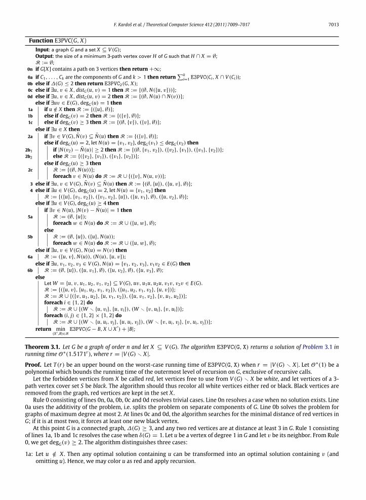
In this section, we design a non-trivial exact algorithm for the 3-PVCPwith running timeO(1.5171n). Our approach tendsto solve a slightly more general problem, where out of a given graph G, given is a subset of vertices X and the goal is to finda 3-path vertex cover set which is vertex disjoint with X .

Problem 3.1. Given a graph G and a set of vertices X , find a minimum 3-path vertex cover set S for G such that S ∩ X = ∅,or report that no such 3-path vertex cover exists.

First, recall that for a case when ∆(G) ≤ 2, a simple linear-time algorithm can be used to solve this problem; we omitthe details. We denote such an algorithm by E3PVC2(G, X).

Our algorithm E3PVC for a general graph uses a branch-and-bound approach. In each step, the algorithm reduces thenumber of vertices of the graph, or increases the size of X . The algorithm is shown on the following figure as recursivefunction E3PVC(G, X). One call of a recursion either solves a trivial case, or creates a rule R which may contain one ormore branchings. One branch (X ′, B) is a pair of subsets of V (G) and reduces the problem to solve E3PVC(G − B, X ∪

X ′), which means that vertices of B are inserted into a constructed 3-path vertex cover and vertices of X ′ are insertedto X .

In the description of the algorithm, we use the following notation. For a vertex v, let N(v) denote the set of allneighbors of v in a graph G. Let N(v) = N(v) ∪ {v}. For a set of vertices S, let N(S) =

u∈S N(u) and let N(S) = N

(S) r S.

F. Kardoš et al. / Theoretical Computer Science 412 (2011) 7009–7017 7013

Function E3PVC(G, X)Input: a graph G and a set X ⊆ V (G);Output: the size of a minimum 3-path vertex cover H of G such that H ∩ X = ∅;R := ∅;

0n if G[X] contains a path on 3 vertices then return +∞;

0a if C1, . . . , Ck are the components of G and k > 1 then return∑k

i=1 E3PVC(Ci, X ∩ V (Ci));0b else if ∆(G) ≤ 2 then return E3PVC2(G, X);0c else if ∃u, v ∈ X, distG(u, v) = 1 then R := {(∅,N({u, v}))};0d else if ∃u, v ∈ X, distG(u, v) = 2 then R := {(∅,N(u) ∩ N(v))};

else if ∃uv ∈ E(G), degG(u) = 1 then1a if u /∈ X then R := {({u},∅)};1b else if degG(v) = 2 then R := {({v},∅)};1c else if degG(v) ≥ 3 then R := {(∅, {v}), ({v},∅)};

else if ∃u ∈ X then2a if ∃v ∈ V (G), N(v) ⊆ N(u) then R := {({v},∅)};

else if degG(u) = 2, let N(u) = {v1, v2}, degG(v1) ≤ degG(v2) then2b1 if |N(v2)− N(u)| ≥ 2 then R := {(∅, {v1, v2}), ({v2}, {v1}), ({v1}, {v2})};2b2 else R := {({v2}, {v1}), ({v1}, {v2})};

else if degG(u) ≥ 3 then2c R := {(∅,N(u))};

foreach v ∈ N(u) do R := R ∪ {({v},N(u, v))};3 else if ∃u, v ∈ V (G), N(v) ⊆ N(u) then R := {(∅, {u}), ({u, v},∅)};4 else if ∃u ∈ V (G), degG(u) = 2, let N(u) = {v1, v2} then

R := {({u}, {v1, v2}), ({v1, v2}, {u}), ({u, v1},∅), ({u, v2},∅)};else if ∃u ∈ V (G), degG(u) ≥ 4 then

if ∃v ∈ N(u), |N(v)− N(u)| = 1 then5a R := (∅, {u});

foreach w ∈ N(u) do R := R ∪ ({u, w},∅);else

5b R := (∅, {u}), ({u},N(u));foreach w ∈ N(u) do R := R ∪ ({u, w},∅);

else if ∃u, v ∈ V (G),N(u) = N(v) then6a R := ({u, v},N(u)), (N(u), {u, v});

else if ∃u, v1, v2, v3 ∈ V (G),N(u) = {v1, v2, v3}, v1v2 ∈ E(G) then6b R := (∅, {u}), ({u, v1},∅), ({u, v2},∅), ({u, v3},∅);

elseLet W = {u, v, u1, u2, v1, v2} ⊆ V (G), uv, u1u, u2u, v1v, v2v ∈ E(G).R := {({u, v}, {u1, u2, v1, v2}), ({u1, u2, v1, v2}, {u, v})};R := R ∪ {({v, u1, u2}, {u, v1, v2}), ({u, v1, v2}, {v, u1, u2})};foreach i ∈ {1, 2} do

R := R ∪ {(W r {u, vi}, {u, vi}), (W r {v, ui}, {v, ui})};foreach (i, j) ∈ {1, 2} × {1, 2} do

R := R ∪ {(W r {u, ui, vj}, {u, ui, vj}), (W r {v, ui, vj}, {v, ui, vj})};return min

(X ′,B)∈RE3PVC(G − B, X ∪ X ′)+ |B|;

Theorem 3.1. Let G be a graph of order n and let X ⊆ V (G). The algorithm E3PVC(G, X) returns a solution of Problem 3.1 inrunning time O∗(1.5171r), where r = |V (G) r X |.

Proof. Let T (r) be an upper bound on the worst-case running time of E3PVC(G, X) when r = |V (G) r X |. Let O∗(1) be apolynomial which bounds the running time of the outermost level of recursion on G, exclusive of recursive calls.

Let the forbidden vertices from X be called red, let vertices free to use from V (G) r X be white, and let vertices of a 3-path vertex cover set S be black. The algorithm should thus recolor all white vertices either red or black. Black vertices areremoved from the graph, red vertices are kept in the set X .

Rule 0 consisting of lines 0n, 0a, 0b, 0c and 0d resolves trivial cases. Line 0n resolves a case when no solution exists. Line0a uses the additivity of the problem, i.e. splits the problem on separate components of G. Line 0b solves the problem forgraphs of maximum degree at most 2. At lines 0c and 0d, the algorithm searches for the minimal distance of red vertices inG; if it is at most two, it forces at least one new black vertex.

At this point G is a connected graph,∆(G) ≥ 3, and any two red vertices are at distance at least 3 in G. Rule 1 consistingof lines 1a, 1b and 1c resolves the case when δ(G) = 1. Let u be a vertex of degree 1 in G and let v be its neighbor. From Rule0, we get degG(v) ≥ 2. The algorithm distinguishes three cases:

1a: Let u /∈ X . Then any optimal solution containing u can be transformed into an optimal solution containing v (andomitting u). Hence, we may color u as red and apply recursion.

7014 F. Kardoš et al. / Theoretical Computer Science 412 (2011) 7009–7017

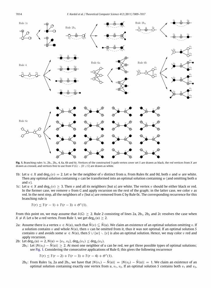
Fig. 1. Branching rules 1c, 2b1 , 2b2 , 4, 6a, 6b and 6c. Vertices of the constructed 3-path vertex cover set S are drawn as black, the red vertices from X aredrawn as crossed, and vertices free to use from V (G) r {X ∪ S} are drawn as white.

1b: Let u ∈ X and degG(v) = 2. Let w be the neighbor of v distinct from u. From Rules 0c and 0d, both v and w are white.Then any optimal solution containing v can be transformed into an optimal solution containingw (and omitting both uand v).

1c: Let u ∈ X and degG(v) ≥ 3. Then v and all its neighbors (but u) are white. The vertex v should be either black or red.In the former case, we remove v from G and apply recursion on the rest of the graph; in the latter case, we color v asred. In the next step, all the neighbors of v (but u) are removed from G by Rule 0c. The corresponding recurrence for thisbranching rule is

T (r) ≤ T (r − 1)+ T (r − 3)+ O∗(1).

From this point on, we may assume that δ(G) ≥ 2. Rule 2 consisting of lines 2a, 2b1, 2b2 and 2c resolves the case whenX = ∅. Let u be a red vertex. From Rule 1, we get degG(u) ≥ 2.

2a: Assume there is a vertex v ∈ N(u), such that N(v) ⊆ N(u). We claim an existence of an optimal solution omitting v. Ifa solution contains v and whole N(u), then v can be omitted from it, thus it was not optimal. If an optimal solution Scontains v and avoids some w ∈ N(u), then S ∪ {w} r {v} is also an optimal solution. Hence, we may color v red andapply recursion.

2b: Let degG(u) = 2, N(u) = {v1, v2}, degG(v1) ≤ degG(v2).2b1: Let |N(v2) − N(u)| ≥ 2. At most one neighbor of u can be red, we get three possible types of optimal solutions;

see Fig. 1. Considering the consecutive applications of Rule 0, this gives the following recurrence

T (r) ≤ T (r − 2)+ T (r − 3)+ T (r − 4)+ O∗(1).

2b2: From Rules 1a, 2a and 2b1, we have that |N(v1) − N(u)| = |N(v2) − N(u)| = 1. We claim an existence of anoptimal solution containing exactly one vertex from u, v1, v2. If an optimal solution S contains both v1 and v2,

F. Kardoš et al. / Theoretical Computer Science 412 (2011) 7009–7017 7015

then S r {v2} ∪ (N(v2) − N(u)) is a solution of size at most |S| avoiding v2. This gives two branches depicted inFig. 1, from which we obtain the following recurrence

T (r) ≤ 2T (r − 2)+ O∗(1).

2c: Let degG(u) = d ≥ 3. An optimal solution either contains all the vertices of N(u) or at most one vertex from N(u) ismissing. This gives 1 + d branches; however Rule 2a forces that in d branches, the consecutive application of Rule 0decreases the problem by one more vertex. Therefore, we obtain the following inequality for T

T (r) ≤ T (r − d)+ d · T (r − d − 1)+ O∗(1).

From this point on, we may assume that there are no red vertices in G, i.e. X = ∅.

3: Let u, v ∈ V (G), N(v) ⊆ N(u). The algorithm uses two branches here. The first covers all solutions containing u. In theopposite case, when u is not in an optimal solution, we claim an existence of an optimal solution also avoiding v: if S is asolution such that u /∈ S and v ∈ S, then S ∪ {u} r {v} is also a solution of size at most |S|. The corresponding recurrencefor this branching is

T (r) ≤ T (r − 1)+ T (r − 3)+ O∗(1),

since from Rule 1 |N(u)| ≥ 2. Moreover, in a case when u and v are colored as red, a consecutive application of Rule 0colors N(u) r {v} as black.

Rule 4 resolves the case δ(G) = 2. Let u be a vertex of degree 2 in G, let v1 and v2 be its neighbors.

4: Clearly, an optimal solution contains either one or two vertices from u, v1, v2, this is depicted in Fig. 1. In two branches,the consecutive application of Rule 0 color at least one more vertex as black, therefore the corresponding recurrence forthis branching rule is

T (r) ≤ 2T (r − 3)+ 2T (r − 4)+ O∗(1).

At this point, we may assume that δ(G) ≥ 3. Rule 5 resolves the case when∆(G) ≥ 4. Let u be a vertex of degree d = ∆(G).

5a: Let v ∈ N(u), |N(v) − N(u)| = 1. We claim that either an optimal solution contains u or there exists an optimalsolution avoiding u and exactly one vertex from N(u). If an optimal solution S avoids u and contains all vertices fromN(u), then S r {v} ∪ (N(v) − N(u)) is also a solution of size at most |S|. Using Rule 3, for each vertex w ∈ N(u), wehave |N(v)− N(u)| ≥ 1, therefore considering a consecutive application of Rule 0 the corresponding recurrence for thisbranching is

T (r) ≤ T (r − 1)+ d · T (r − 1 − d − 1)+ O∗(1).

5b: The algorithm branches over the following cases. Each optimal solution either contains u, or at least d− 1 vertices fromN(u). From Rule 5a, we have that |N(v) − N(u)| ≥ 2 for each neighbor v of u. Hence, if u and v are both red, thenthe consecutive application of Rule 0 gives at least two more black vertices besides those from N(u). Therefore, thecorresponding recurrence is

T (r) ≤ T (r − 1)+ T (r − d − 1)+∆ · T (r − 1 − d − 2)+ O∗(1).

At this point, we may assume that G is a cubic graph, i.e. each vertex has degree 3.

6a: Let u, v be vertices of G such that N(u) = N(v). Since G is cubic, |{u, v} ∪ N(u)| = 5. If an optimal solution contains atmost two of these five vertices, this can be only due to {u, v}. Any optimal solution containing at least three of these fivevertices can be transformed to one containing N(u) and avoiding u and v. The corresponding branching rule is depictedin Fig. 1. This leads to the recurrence

T (r) ≤ 2T (r − 5)+ O∗(1).

6b: Let vertices u1, u2, u3 form a cycle of length 3 in G; let vi be the neighbor of ui not from {u1, u2, u3}. From Rule 3, weknow that v1, v2, v3 are pairwise distinct. If S is solution containing v1, u2, and u3, then S r {u2} ∪ (N(u2) − N(u)) isa solution of size at most |S|. Therefore, we only search for optimal solutions which either contain u1, or avoid u1 andcontain precisely two of its neighbors. The corresponding branching rule is depicted in Fig. 1 and leads to the recurrence

T (r) ≤ T (r − 1)+ 2T (r − 5)+ T (r − 6)+ O∗(1).

6c: Let u, v be neighbors in G. From Rule 6b, N(u)∩N(v) = ∅. Let N(u) = {u1, u2, v} and N(v) = {v1, v2, u}. From Rule 6a,each ui (i = 1, 2) is adjacent to at most one vertex from {v1, v2} and vice versa. Consider the six vertices in N(u)∪N(v).If a solution S contains u and v together with u1, then S r {u} ∪ {u2} is a solution of the same size. Hence, if an optimal

7016 F. Kardoš et al. / Theoretical Computer Science 412 (2011) 7009–7017

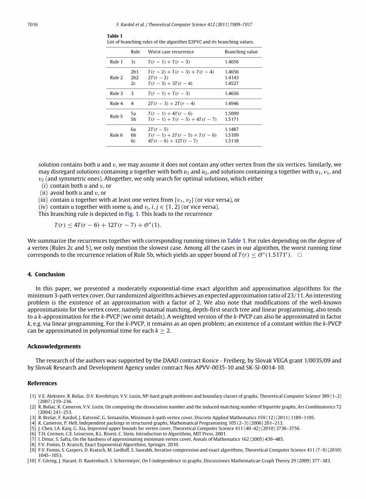
Table 1List of branching rules of the algorithm E3PVC and its branching values.

Rule Worst case recurrence Branching value

Rule 1 1c T (r − 1)+ T (r − 3) 1.4656

Rule 22b1 T (r − 2)+ T (r − 3)+ T (r − 4) 1.46562b2 2T (r − 2) 1.41432c T (r − 3)+ 3T (r − 4) 1.4527

Rule 3 3 T (r − 1)+ T (r − 3) 1.4656

Rule 4 4 2T (r − 3)+ 2T (r − 4) 1.4946

Rule 5 5a T (r − 1)+ 4T (r − 6) 1.50995b T (r − 1)+ T (r − 5)+ 4T (r − 7) 1.5171

Rule 66a 2T (r − 5) 1.14876b T (r − 1)+ 2T (r − 5)+ T (r − 6) 1.51096c 4T (r − 6)+ 12T (r − 7) 1.5118

solution contains both u and v, we may assume it does not contain any other vertex from the six vertices. Similarly, wemay disregard solutions containing u together with both u1 and u2, and solutions containing u together with u1, v1, andv2 (and symmetric ones). Altogether, we only search for optimal solutions, which either(i) contain both u and v, or(ii) avoid both u and v, or(iii) contain u together with at least one vertex from {v1, v2} (or vice versa), or(iv) contain u together with some ui and vj, i, j ∈ {1, 2} (or vice versa).This branching rule is depicted in Fig. 1. This leads to the recurrence

T (r) ≤ 4T (r − 6)+ 12T (r − 7)+ O∗(1).

We summarize the recurrences together with corresponding running times in Table 1. For rules depending on the degree ofa vertex (Rules 2c and 5), we only mention the slowest case. Among all the cases in our algorithm, the worst running timecorresponds to the recurrence relation of Rule 5b, which yields an upper bound of T (r) ≤ O∗(1.5171r). �

4. Conclusion

In this paper, we presented a moderately exponential-time exact algorithm and approximation algorithms for theminimum3-path vertex cover. Our randomized algorithmachieves an expected approximation ratio of 23/11. An interestingproblem is the existence of an approximation with a factor of 2. We also note that modifications of the well-knownapproximations for the vertex cover, namely maximal matching, depth-first search tree and linear programming, also tendsto a k-approximation for the k-PVCP (we omit details). A weighted version of the k-PVCP can also be approximated in factork, e.g. via linear programming. For the k-PVCP, it remains as an open problem; an existence of a constant within the k-PVCPcan be approximated in polynomial time for each k ≥ 2.

Acknowledgements

The research of the authors was supported by the DAAD contract Kosice - Freiberg, by Slovak VEGA grant 1/0035/09 andby Slovak Research and Development Agency under contract Nos APVV-0035-10 and SK-SI-0014-10.

References

[1] V.E. Alekseev, R. Boliac, D.V. Korobitsyn, V.V. Lozin, NP-hard graph problems and boundary classes of graphs, Theoretical Computer Science 389 (1–2)(2007) 219–236.

[2] R. Boliac, K. Cameron, V.V. Lozin, On computing the dissociation number and the induced matching number of bipartite graphs, Ars Combinatorics 72(2004) 241–253.

[3] B. Brešar, F. Kardoš, J. Katrenič, G. Semanišin, Minimum k-path vertex cover, Discrete Applied Mathematics 159 (12) (2011) 1189–1195.[4] K. Cameron, P. Hell, Independent packings in structured graphs, Mathematical Programming 105 (2–3) (2006) 201–213.[5] J. Chen, I.A. Kanj, G. Xia, Improved upper bounds for vertex cover, Theoretical Computer Science 411 (40–42) (2010) 3736–3756.[6] T.H. Cormen, C.E. Leiserson, R.L. Rivest, C. Stein, Introduction to Algorithms, MIT Press, 2001.[7] I. Dinur, S. Safra, On the hardness of approximating minimum vertex cover, Annals of Mathematics 162 (2005) 439–485.[8] F.V. Fomin, D. Kratsch, Exact Exponential Algorithms, Springer, 2010.[9] F.V. Fomin, S. Gaspers, D. Kratsch, M. Liedloff, S. Saurabh, Iterative compression and exact algorithms, Theoretical Computer Science 411 (7–9) (2010)

1045–1053.[10] F. Göring, J. Harant, D. Rautenbach, I. Schiermeyer, On f-independence in graphs, Discussiones Mathematicae Graph Theory 29 (2009) 377–383.

F. Kardoš et al. / Theoretical Computer Science 412 (2011) 7009–7017 7017

[11] J. Kneis, A. Langer, P. Rossmanith, A fine-grained analysis of a simple independent set algorithm, in: FSTTCS, 2009, pp. 287–298.[12] L. Lovász, On decompositions of graphs, Studia Scientiarum Mathematicarum Hungarica 1 (1966) 237–238.[13] V.V. Lozin, D. Rautenbach, Some results on graphs without long induced paths, Information Processing Letters 88 (4) (2003) 167–171.[14] M. Novotný, Design and analysis of a generalized canvas protocol, in: Proceedings of WISTP 2010, in: Lecture Notes in Computer Science, vol. 6033,

2010, pp. 106–121.[15] Y. Orlovich, A. Dolguib, G. Finkec, V. Gordond, F. Wernere, The complexity of dissociation set problems in graphs, Discrete Applied Mathematics 159

(13) (2011) 1352–1366.[16] C.H. Papadimitriou, M. Yannakakis, The complexity of restricted spanning tree problems, Journal of ACM 29 (2) (1982) 285–309.[17] J. Robson, Finding a maximum independent set in time O(2(n/4)) (January 2001). URL: http://www.labri.fr/perso/robson/mis/techrep.html.[18] M. Wahlström, Algorithms, measures and upper bounds for satisfiability and related problems, Ph.D. Thesis, Linköping University, Sweden, 2007.[19] M. Yannakakis, Node-deletion problems on bipartite graphs, SIAM Journal on Computing 10 (2) (1981) 310–327.