Computer-Aided Design 48 (2014) 39–41

Contents lists available at ScienceDirect

Computer-Aided Design

journal homepage: www.elsevier.com/locate/cad

Technical note

On computing the shortest path in a multiply-connected domainhaving curved boundariesXiangzhi Wei, Ajay Joneja ∗

Department of IELM, HKUST, Clear Water Bay, Kowloon, Hong Kong

a r t i c l e i n f o

Article history:Received 11 August 2013Accepted 16 November 2013

Keywords:Shortest pathCurve obstaclesMultiply-connected curvesVisibility graphFreeform curves

a b s t r a c t

This submission is a communication related to a recently published article in Computer-Aided Designjournal, titled ‘‘Shortest path in amultiply-connected domain having curved boundaries’’.We point out anerror in estimating the time complexity of the algorithm proposed in that paper, using a simple example.We also illustrate,with a different example, that an ostensibly time-saving schemeused by that algorithm,called exterior region elimination, cannot be applied in general to derive the correct shortest interior path.Finally, we propose an alternate algorithm that solves the same problem with an improved worst-caserunning time.

© 2013 Elsevier Ltd. All rights reserved.

1. Background

Computing a shortest interior path (SIP) in amultiply connecteddomain (MCD) having curved boundaries is a fundamental andinteresting problem in geometry and engineering. Recently,Bharath Ram and Ramanathan [1] proposed an algorithm forcomputing an SIP from a starting point S to a destination pointE in an MCD. They use the observation that the SIP is composedof a sequence of segments that are either bitangents (BTs) in theinterior of the MCD, or concave portions of curves on the boundaryof the MCD. Their algorithm is an extension of their earlier workfor the analogous problem in a simply-connected domain (SCD)having curved boundaries and no holes [2]. An advantage of thealgorithmpresented in [1] is that it can bepractically implemented.In this communication, we discuss some issues related to thealgorithm and the runtime analysis presented in [1]. Furthermore,we present a simple method to improve the worst-case runtime.In the following, we will use the same terminology as in [1] whenpossible.

Chen and Wang [3] showed that an SIP can be computed inO(K 2) time using the visibility graph of anMCD in which each loopis a pseudodisk of O(1) complexity, and K is the total descriptioncomplexity of the MCD. Later, they provided an O(K + h log1+ε h+

k) time algorithm for a more general version of the problem inwhich each of the h loops is a splinegon, K is the total number

∗ Corresponding author.E-mail addresses: xiangzhi.science@gmail.com (X. Wei), joneja@ust.hk

(A. Joneja).

0010-4485/$ – see front matter© 2013 Elsevier Ltd. All rights reserved.http://dx.doi.org/10.1016/j.cad.2013.11.001

of edges (each of constant complexity) in all the splinegons, andthe parameter k is bounded by O(h2) [4]. Their approach reducesthe initial problem to that of an instance of an MCD with h convexloops, and then applies Dijkstra’s algorithm to the visibility graphof the reduced MCD. The algorithm is difficult to implement sinceit uses some advanced data structures. For example, it utilizesthe triangulation scheme on Jordan curves from [5], which inturn requires Chazelle’s linear time triangulation [6] of a simplepolygon. This seminal paper has proven to be impractical toimplement so far [7].

Without using visibility graphs, Hershberger et al. [8] recentlyproposed an approach using the continuous Dijkstra paradigm ona conforming subdivision to solve the problem in near-optimalO(K log K) time. They require that the arcs possess the propertythat their pairwise bisector intersection can be computed inat most O(log K) time. The paper adapted the approach firstdeveloped by the same group for polygonal domains [9]. However,it has been pointed out that implementing the approach in [9] isimpractical (see for instance [10]).

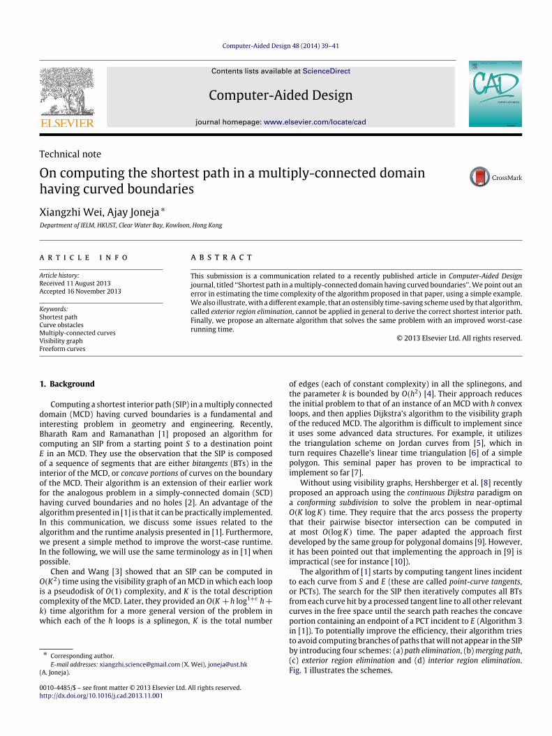
The algorithm of [1] starts by computing tangent lines incidentto each curve from S and E (these are called point-curve tangents,or PCTs). The search for the SIP then iteratively computes all BTsfrom each curve hit by a processed tangent line to all other relevantcurves in the free space until the search path reaches the concaveportion containing an endpoint of a PCT incident to E (Algorithm 3in [1]). To potentially improve the efficiency, their algorithm triesto avoid computing branches of paths thatwill not appear in the SIPby introducing four schemes: (a) path elimination, (b)merging path,(c) exterior region elimination and (d) interior region elimination.Fig. 1 illustrates the schemes.

40 X. Wei, A. Joneja / Computer-Aided Design 48 (2014) 39–41

Fig. 1. (a) Path elimination: the red path will be eliminated. (b) Path merging: the green path will use the dotted blue BT to propagate further; the subtree (of the tree datastructure for path merging) rooted at the node representing the dotted blue BT and containing all the traversed subpaths beyond it will be added to the node representingthe dotted green BT; subsequently the path length information for each of the nodes in this newly added subtree is updated. (c) Exterior region elimination: the extended BTshown as a dashed line induces an elimination region (gray area). (d) Interior region elimination: the eliminated region is shown in gray. (For interpretation of the referencesto colour in this figure legend, the reader is referred to the web version of this article.)

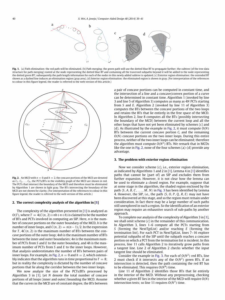
Fig. 2. AnMCDwith n = 0 and h = 2, the concave portions of theMCD are denotedas C1, C2, . . . CN , the PCTs/BTs in the visibility graph of the MCD are shown in red.The PCTs that intersect the boundary of the MCD and therefore must be eliminatedby Algorithm 1 are shown in light gray. The BTs intersecting the boundary of theMCD are not shown for clarity. (For interpretation of the references to colour in thisfigure legend, the reader is referred to the web version of this article.)

2. The correct complexity analysis of the algorithm in [1]

The complexity of the algorithm presented in [1] is analyzed asO(T ), where T = 4(C(n, 2)+nh+n+h) is claimed to be the numberof BTs and PCTs involved in computing an SIP. Here, n is the num-ber of concave portions on the outer boundary of the MCD, h is thenumber of inner loops, and C(n, 2) = n(n−1)/2. In the expressionfor T , 4C(n, 2) is the maximum number of BTs between the con-cave portions of the outer loop; 4nh is themaximumnumber of BTsbetween the inner and outer boundaries; 4n is themaximumnum-ber of PCTs from S and E to the outer boundary, and 4h is the max-imum number of PCTs from S and E to the inner loops. However,that analysis underestimates the number of BTs between pairs ofinner loops. For example, in Fig. 2, n = 0 and h = 2, which ostensi-bly indicates that the algorithm runs in time proportional to T = 8;but in reality the complexity is dictated by the number of concaveportions that lie along the corridor between the two inner loops.

We now analyze the size of the PCTs/BTs processed byAlgorithm 3 in [1]. Let N denote the total number of concaveportions of all loops (inner and outer) bounding the MCD. Assumethat the curves in theMCD are of constant degree, the BTs between

a pair of concave portions can be computed in constant time, andthe intersection of a line and a concave/convex portion of a curvecan be determined in constant time. Algorithm 1 (invoked by line3 and line 5 of Algorithm 3) computes as many as 4N PCTs startingfrom S and E. Algorithm 2 (invoked by line 11 of Algorithm 3)computes the BTs between the concave portions of the two loopsand retains the BTs that lie entirely in the free space of the MCD.In Algorithm 2, line 8 computes all the BTs (possibly intersectingthe boundary of the MCD) between the current loop and all theother loops that have not yet been eliminated by schemes (c) and(d). As illustrated by the example in Fig. 2, it must compute O(N)BTs between the current concave portion Ci and the remainingO(N) concave portions on the two inner loops. During this entireprocess, neither of the two inner loops can be eliminated; thereforethe algorithm must compute O(N2) BTs. We remark that in MCDslike the one in Fig. 2, none of the four schemes (a)–(d) provide anyadvantage.

3. The problem with exterior region elimination

Now we consider scheme (c), i.e., exterior region elimination,as indicated by Algorithms 1 and 2 in [1]. Lemma 4 in [1] identifiespaths that cannot be (part of) an SIP and excludes them fromfurther expansion. However, it is not clear how the lemma canbe used to eliminate a closed region. For example, suppose thatat some stage in the algorithm, the shaded region enclosed by thepath ⟨S, A, B, C, . . . ,M,N⟩ in Fig. 3 has been identified by Lemma4. However, the SIP, i.e., the path ⟨S,O, P,Q , R, E⟩ may not havebeen discovered at this stage, and so the regionmust remain underconsideration. In fact there may be a large number of such pathsstill unexplored in such a region. So the identification of an exteriorregion may require an exhaustive search of sub-paths by anotherapproach.

To complete our analysis of the complexity of Algorithm3 in [1],we shall omit scheme (c) in the remainder of this communication.In Algorithm 3, lines 1–6 compute all the PCTs starting fromS (forming the NextTgtList) and/or reaching E (forming thetermination list). For each PCT in NextTgtList, lines 7–16 explorepotential subpaths of the SIP until the subpath reaches a concaveportion onwhich a PCT from the termination list is incident. In thisprocess, line 11 calls Algorithm 2 to iteratively grow paths froma tangent line. Line 2 of Algorithm 2 checks whether the inputtangent line should be eliminated.

Consider the example in Fig. 3. For each of O(N2) red BTs, line2 must check if it intersects any of the O(N2) green BTs. If anintersection is detected, then the path containing the red BT hasto be eliminated. This requires O(N4) time.

Line 11 of Algorithm 2 identifies those BTs that lie entirelyin the interior of the MCD. Without any preprocessing, checkingwhether a given BT lies in the interior of theMCDwill requireO(N)intersection tests; so line 11 requires O(N3) time.

X. Wei, A. Joneja / Computer-Aided Design 48 (2014) 39–41 41

Fig. 3. AnMCDwithN concave regions, withN/4∗(N/4−C) green BTs, where C issome small integer, and N/4∗N/4 red BTs in the interior of theMCD. The extendedportions of the PCTs are shown in dashed lines. Some BTs that are irrelevant for ouranalysis are not shown. (For interpretation of the references to colour in this figurelegend, the reader is referred to the web version of this article.)

4. Discussion

It is claimed in [1] that their technique has the advantage ofbeing able to compute the SIP without using either the visibilitygraph or Dijkstra’s algorithm. In the following, we shall illustratehow a simple variation of their algorithm, using visibility graphsand a Dijkstra-style search, can yield significantly improvedworst-case performance.

Computing all PCTs/BTs in the interior of theMCD (as Algorithm2 must, in the worst case) and then sorting the endpoints of BTslying on each loop by parameter value is sufficient for computingthe visibility graph of the MCD [4]. The nodes of this graphare the endpoints of the BTs, and its arcs are the BTs and theconcave portion between any two consecutive nodes on eachcurve. The number of nodes and arcs in the visibility graph are bothbounded by O(N2). We can therefore use Dijkstra’s algorithm on

the visibility graph to compute an SIP using a simple min-priorityqueue [11] in O(N2 logN) time. As shown above, the PCTs/BTs inthe free space can be obtained in O(N3) by a brute force algorithm.The total number of endpoints of the BTs is bounded by O(N2);therefore the time required to sort the endpoints on each curve isO(N2 logN) time. This relatively simple variation of the algorithmof [1] reduces the worst case complexity from O(N4) to O(N3).Another advantage of directly using this method is that we avoidhaving to determine how to efficiently use the schemes (a)–(d),e.g., identifying interior eliminated regions, merging paths, etc.We remark that allowing for more sophisticated techniques canprovide even more significant improvements in solving the SIPproblem in MCDs [4], although the practical implementation ofthat scheme is comparatively difficult.

Acknowledgments

Part of this research was supported by the RGC GRF grant #613312, and by the Department of IELM, HKUST.

References

[1] Bharath Ram S, RamanathanM. Shortest path in amultiply-connected domainhaving curved boundaries. Comput-Aided Des 2013;45:723–32.

[2] Bharath Ram S, Ramanathan M. The shortest path in a simply-connecteddomain having a curved boundary. Comput-Aided Des 2011;43(8):923–33.

[3] Chen DZ, Wang H. Computing shortest paths amid pseudodisks. In: Proceed-ings of the 22nd annual ACM–SIAM symposium on discrete algorithms. 2011.p. 309–26.

[4] Chen DZ, Wang H. Computing shortest paths among curved obstaclesin the plane. In: Proceedings of the twenty-ninth annual symposium oncomputational geometry. 2013. p. 369–78.

[5] Bar-Yehuda R, Chazelle B. Triangulating disjoint Jordan chains. Internat JComput Geom Appl 1994;4(4):475–81.

[6] Chazelle B. Triangulating a simple polygon in linear time. Discrete ComputGeom 1991;6(5):485–524.

[7] Bishop CJ. Conformal mapping in linear time. Discrete Comput Geom 2010;44(2):330–428.

[8] Hershberger J, Suri S, Yıldız H. A near-optimal algorithm for shortest pathsamong curved obstacles in the plane. In: Proceedings of the 29th annualsymposium on computational geometry. 2013. p. 359–68.

[9] Hershberger J, Suri S. An optimal algorithm for Euclidean shortest paths in theplane. SIAM J Comput 1999;28(6):2215–56.

[10] Gao Y, Zheng B, Chen G, Chen C, Li Q. Continuous nearest-neighbor search inthe presence of obstacles. ACM Trans Database Syst 2011;36(2):9:1–9:43.

[11] Cormen TH, Leiserson CE, Rivest RL, Stein C. Introduction to algorithms. 3rd ed.Cambridge, MA: MIT Press; 2009.