Embed Size (px)
Citation preview
On domain knowledge and feature selection using a supportvector machine
O®r Barzilay 1, V.L. Brailovsky *
Department of Computer Science, Tel Aviv University, 69978 Ramat Aviv, Israel
Received 8 July 1998; received in revised form 24 November 1998
Abstract
The basic principles of a support vector machine (SVM) are analyzed. The problem of feature selection while using
an SVM is speci®cally addressed. An approach to constructing a kernel function which takes into account some domain
knowledge about a problem and thus essentially diminishes the number of noisy parameters in high dimensional feature
space is suggested. Its application to Texture Recognition is described. Ó 1999 Elsevier Science B.V. All rights re-
served.
Keywords: Domain knowledge; Feature selection; Support vector machine; Texture recognition
1. Introduction
A Support Vector Machine (SVM) is a univer-sal learning machine developed in recent years.SVMs are known to give good results in manyPattern Recognition (PR) problems. The basicprinciples of an SVM according to Guyon et al.(1992) and Cortes and Vapnik (1995) and Vapnik(1995) are as follows (we consider here a two-classproblem):1. The SVM performs a nonlinear mapping of the
input vectors (objects) from the input space Rd
into a high dimensional feature space H ; themapping is determined by a kernel function.
2. It ®nds a linear decision rule in the featurespace H in the form of an optimal separating
plane, which is the one that leaves the widestmargin between the decision boundary andthe input vectors mapped into H .
3. This plane is found by solving the followingconstrained quadratic programming problem:
Maximize W �a�
�Xn
i�1
ai ÿ 1
2
Xn
i�1
Xn
j�1
aiajyiyjK�xi; xj� �1�
under the constraintsPn
i�1 aiyi � 0 and06 ai6C for i � 1; 2; . . . ; n where xi 2 Rd arethe training sample set (TSS) vectors, andyi 2 fÿ1;�1g the corresponding class labels. Cis a constant needed for nonseparable classes;K�u; v� is a kernel function de®ned in 6.
4. The separating plane is constructed from thoseinput vectors, for which ai 6� 0. These vectorsare called support vectors and reside on theboundary margin. The number of support vec-tors determines the accuracy and speed of theSVM.
Pattern Recognition Letters 20 (1999) 475±484
* Corresponding author. Tel.: +972-3-6490440; fax: +972-3-
640-9357; e-mail: [email protected] E-mail: [email protected]
www.elsevier.nl/locate/patrec
0167-8655/99/$ ± see front matter Ó 1999 Elsevier Science B.V. All rights reserved.
PII: S 0 1 6 7 - 8 6 5 5 ( 9 9 ) 0 0 0 1 4 - 8
5. Mapping the separating plane back into the in-put space Rd , gives a separating surface whichforms the following nonlinear decision rule:
y�x� � signXxi2sv
aiyiK�x; xi�"
� b
#: �2�
Here sv denotes the set of support vectors.6. K�u; v� is an inner product in the feature space
H which may be de®ned as a kernel functionin the input space. Conditions required are thatthe kernel K�u; v� be a symmetric functionwhich satis®es the following general positivityconstraint:ZZ
Rd
K�u; v�g�u�g�v�dudv > 0; �3�
which is valid for all g 6� 0 for whichRg2�u�du <1 (Mercer's theorem).
7. The choice of the kernel K�u; v� determines thestructure of the feature space H . A kernel whichsatis®es (3) may be presented in the form
K�u; v� �X
k
akwk�u�wk�v�; �4�
where ak are positive scalars and the functionswk�� represent a basis in the space H .
8. Guyon et al. (1992) and Vapnik (1995) considerthree types of support vector machines:· Polynomial SVM:
K�u; v� � ��u; v� � 1�d : �5�This type of machine describes the mappingof an input space into the feature space thatcontains all products uiviujvjukvk . . . up todegree d.
· Radial Basis Function SVM:
Kc�u; v� � expfÿcjuÿ vj2g: �6�This type of machine forms a separation ruleaccording to radial hyperplanes.
· Two-layer neural network SVM:
K�u; v� � tanh�w�u; v� � c�: �7�This type of machine generates a kind oftwo±layer neural network without backpropagation.
9. The kernel K�u; v� should be chosen a priori.Other parameters of the decision rule (2) are de-
termined by calculating (1), i.e. the set of nu-merical parameters faign
1 which determines thesupport vectors and the scalar b.
The success of the SVM in many applied PRproblems surprised the PR community since theprinciples of the SVM somehow contradict thegenerally held intuitions and beliefs. The usualapproach suggests that there is a small number offeatures which may be obtained with the help offeature selection and extraction methods. We mapthe TSS into the space based on these features, i.e.into a space with dimensionality much smallerthan the original one, and then try to ®nd a goodclassi®cation rule in this feature space.
In the SVM a kind of inverse procedure is used.Instead of decreasing dimensionality we map theTSS into a space of very high dimensionality, i.e.we add a great number of new features withoutchecking their e�ciency, and ®nd a classi®cationrule with some optimal properties in this featurespace. The success of the SVM in solving PRproblems raises the question: Are feature selectionand extraction procedures needed when usingSVM?
This article examines the above question. InSection 2 we analyze a synthetic problem in whichwe check how fast results deteriorate when thedimensionality of input space increases, providedthe TSS size is ®xed. We compare the classi®cationresults of the SVM with those obtained by tradi-tional classi®ers.
In Sections 3 and 4 we consider some naturalproblems of Texture Recognition (TR) when thetexture is generated with the help of generally ac-cepted MRF model. So, it is another example of aproblem with many weak features in the inputspace (a feature is a pixel value).
We consider how to de®ne a kernel K�u; v� thattakes into account domain knowledge (that thesolution is determined by the interaction ofneighbor pixels), and as a result, essentially di-minishes the number of ``noisy features'' in thefeature space H (in comparison to the standardde®nition of kernel functions (5)±(7)).
In recent years there was a number of articlesdevoted to study of connection between domainknowledge and the form of kernel function. E.g. inScholkoph et al. (1997) some kernels that take into
476 O. Barzilay, V.L. Brailovsky / Pattern Recognition Letters 20 (1999) 475±484
account interactions only within a certain neigh-borhood of pixels are considered (so called pi-ramidal receptive ®elds) and an improvement ofthe results of a digit recognition problem is dem-onstrated. Our approach is close to one acceptedin this paper. At the same time we consider an-other problem (TR) and other speci®c forms of thekernel functions. We demonstrate that the usage ofsuch kernels permits solving some TR problemsthat cannot be solved with the help of standardkernel functions.
As demonstrated by Vapnik (1995), the ratio ofthe number of support vectors to the TSS size is anupper bound for the error rate estimate obtainedusing the leave-one-out procedure. It may lead oneto estimate the quality of a solution by this ratio.In Section 3 we show that there are some ``naturalproblems'' like TR where this upper bound is veryfar from the real error estimate and therefore is aninadequate estimate.
2. Patterns with many weak features
To check the ability of an SVM to cope with aproblem where a large number of weak featuresare involved, we created a synthetic database ofnormally distributed vectors.
2.1. Normally distributed vectors
Two classes of vectors were generated accordingto the general multivariate normal density func-tion:
p�x� � 1
�2p�d=2jRj1=2
� exp
�ÿ 1
2�xÿ li�tRÿ1�xÿ li�
�; i � 1; 2;
�8�where x is a d component vector, li are the dcomponent mean vectors, and R is the d � d co-variance matrix which is identical for both classes.
In the case of two classes with equal covariancematrices and a priori probabilities, the optimaldecision rule can be stated very simply (see Dudaand Hart, 1973): To classify a vector x, measure
the squared Mahalanobis distance �xÿ li�tRÿ1�xÿli� from x to each of the mean vectors, and assign xto the category of the closest mean. Formally theoptimal classi®cation function is
F �x� � sign��l1 ÿ l2�tRÿ1x
ÿ 1
2�lt
1Rÿ1l1 ÿ lt
2Rÿ1l2��: �9�
This classi®cation rule is called linear discrimi-nant analysis (LDA), because the decision func-tion is linear.
Usually in classi®cation problems, the values ofthe mean vectors and the covariance matrix arenot known. One way of evaluating these values isby using the maximum likelihood method whichgives the well known (see Anderson, 1958) esti-mates for li and R:
l̂i �1
n
Xxk2wi
xk; �10�
R̂ � 1
2n
X2
i�1
Xxk2wi
�xk ÿ l̂i��xk ÿ l̂i�t; �11�
where n is the number of samples from each classw1 and w2. According to Duda and Hart (1973), asthe TSS size �2n� decreases the estimates for li andR lose accuracy, and when 2n is less than the di-mension of the input vectors, the sample covari-ance matrix is singular. This, of course, causes ahigh error rate and failure of the classi®er since thecovariance matrix cannot be inverted.
Friedman (1989) suggested a method to regu-larize the covariance matrix, using the followingequation:
R̂�k� � �1ÿ k�R̂� kd
trace�R̂�I ; �12�
where k is a regularization parameter (06 k6 1), dis the dimension of the input space, trace�R� is thesum of elements on the diagonal of the covariancematrix R, and I is the identity matrix.
This approach is called regularized discriminantanalysis (RDA). When k � 0 we get the LDAclassi®er, and when k � 1, the RDA approachcorresponds with the nearest means classi®erwhere the input pattern is assigned to the classwith the closest mean.
O. Barzilay, V.L. Brailovsky / Pattern Recognition Letters 20 (1999) 475±484 477
2.2. Test results
We generated a training sample set containingtwo classes of vectors. The vectors were distributedaccording to multivariate normal density func-tions. Both classes had the same covariance matrixR but di�erent mean vectors l1 and l2:
R � diagf83; 83; 83; 120; 333; 333; 50; r2; . . . ; r2g;l1 � �ÿ5; 0; 10;ÿ2; 25;ÿ5; 7:75; l; . . . ;l�;l2 � �5; 10; 0; 10; 5;ÿ25; 0; l; . . . ; l�;where l � 10 and r2 � 100:
The ®rst seven coordinates in l1 and l2 aredi�erent and serve as strong features; all othercoordinates are identical and serve as noisy fea-tures. The two classes are not separable; there arevectors from one class that lie within the decisionarea of the other class and vice versa. The minimalerror rate for the above distribution parametersmay be easily calculated (Duda and Hart, 1973)and is about 7.4%. We applied an orthonormalmatrix to the generated vectors. The resultingvectors had features that are actually weightedsums of the features of the original vectors,meaning that all their features were weak.
We used vectors with up to 900 features inorder to check the feature extraction of the SVM.In all cases the generated TSS contained 90 vec-tors from each class. The support vector machinebuilt a classi®cation rule according to the TSS.The classi®cation was checked using a test set of1000 vectors from each class, distributed accord-ing to the same multivariate normal densityfunctions.
We compared the error rate with the classi®-cation results obtained by using LDA and RDAclassi®ers, where the values of the mean vector andthe covariance matrix were estimated by (10)±(12)
accordingly. For the RDA method we chose foreach test the regularization parameter k whichproduced best classi®cation results.
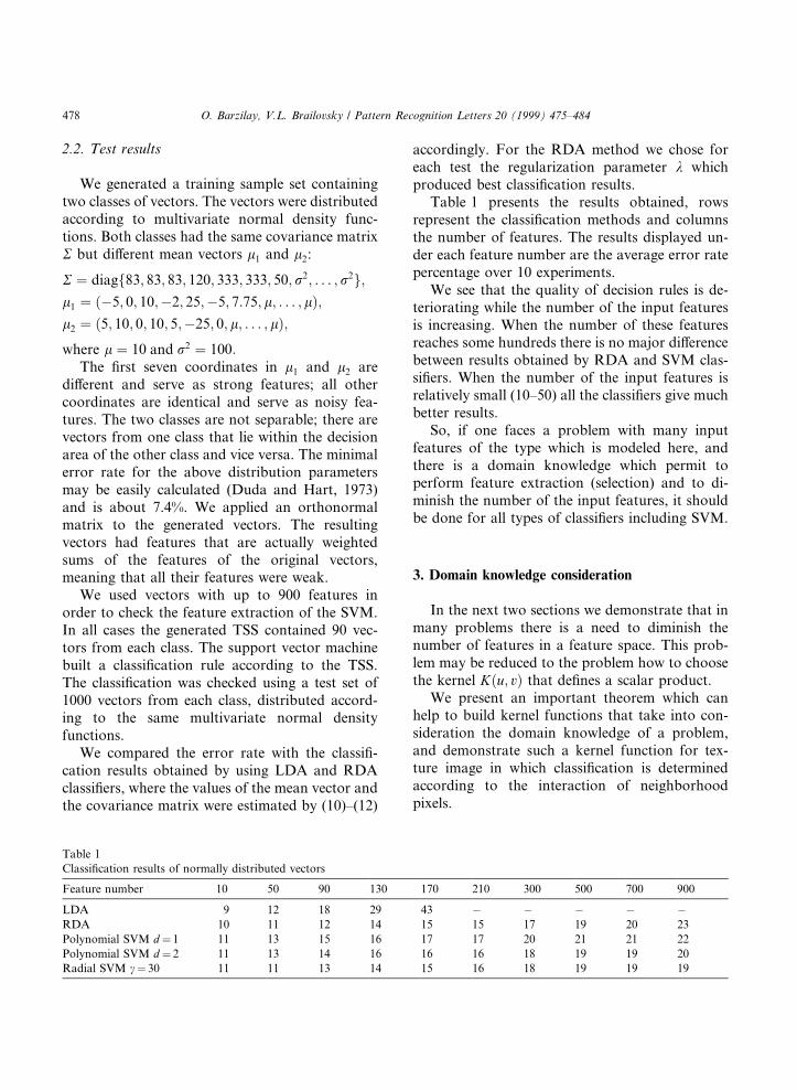
Table 1 presents the results obtained, rowsrepresent the classi®cation methods and columnsthe number of features. The results displayed un-der each feature number are the average error ratepercentage over 10 experiments.
We see that the quality of decision rules is de-teriorating while the number of the input featuresis increasing. When the number of these featuresreaches some hundreds there is no major di�erencebetween results obtained by RDA and SVM clas-si®ers. When the number of the input features isrelatively small (10±50) all the classi®ers give muchbetter results.
So, if one faces a problem with many inputfeatures of the type which is modeled here, andthere is a domain knowledge which permit toperform feature extraction (selection) and to di-minish the number of the input features, it shouldbe done for all types of classi®ers including SVM.
3. Domain knowledge consideration
In the next two sections we demonstrate that inmany problems there is a need to diminish thenumber of features in a feature space. This prob-lem may be reduced to the problem how to choosethe kernel K�u; v� that de®nes a scalar product.
We present an important theorem which canhelp to build kernel functions that take into con-sideration the domain knowledge of a problem,and demonstrate such a kernel function for tex-ture image in which classi®cation is determinedaccording to the interaction of neighborhoodpixels.
Table 1
Classi®cation results of normally distributed vectors
Feature number 10 50 90 130 170 210 300 500 700 900
LDA 9 12 18 29 43 ÿ ÿ ÿ ÿ ÿRDA 10 11 12 14 15 15 17 19 20 23
Polynomial SVM d � 1 11 13 15 16 17 17 20 21 21 22
Polynomial SVM d � 2 11 13 14 16 16 16 18 19 19 20
Radial SVM c� 30 11 11 13 14 15 16 18 19 19 19
478 O. Barzilay, V.L. Brailovsky / Pattern Recognition Letters 20 (1999) 475±484
3.1. Sum of kernel functions
Theorem. If a kernel function K�x; y� can bepresented in the form
K�x; y� �Xm
i�1
Ki�x; y�; �13�
where each of the functions Ki�x; y� complies withthe condition of Mercer's theorem (3), then K�x; y�also complies with that condition and may be used asa kernel function for an SVM.
The proof is straightforward.
3.2. SVM neighborhood kernel function
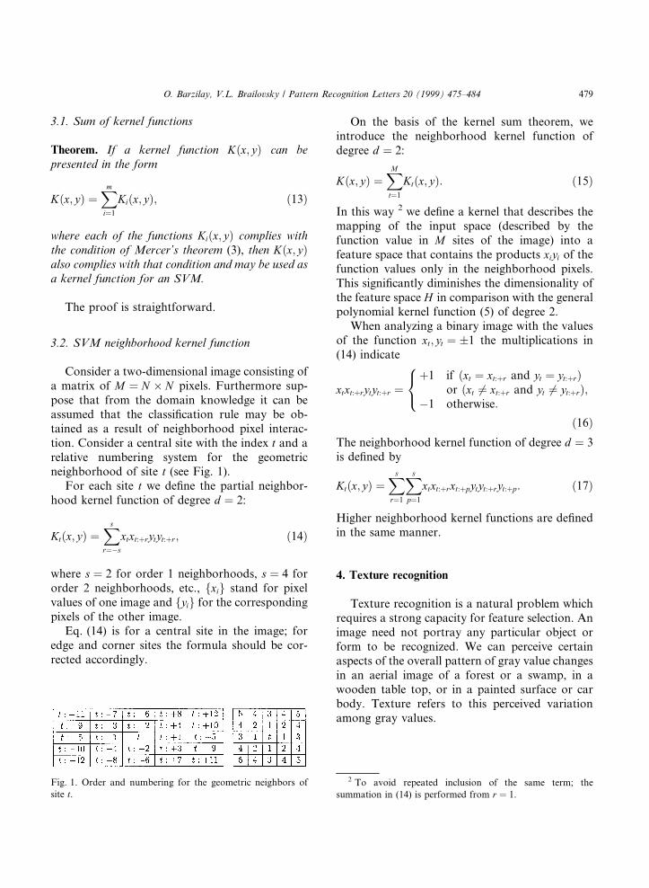
Consider a two-dimensional image consisting ofa matrix of M � N � N pixels. Furthermore sup-pose that from the domain knowledge it can beassumed that the classi®cation rule may be ob-tained as a result of neighborhood pixel interac-tion. Consider a central site with the index t and arelative numbering system for the geometricneighborhood of site t (see Fig. 1).
For each site t we de®ne the partial neighbor-hood kernel function of degree d � 2:
Kt�x; y� �Xs
r�ÿs
xtxt:�rytyt:�r; �14�
where s � 2 for order 1 neighborhoods, s � 4 fororder 2 neighborhoods, etc., fxig stand for pixelvalues of one image and fyig for the correspondingpixels of the other image.
Eq. (14) is for a central site in the image; foredge and corner sites the formula should be cor-rected accordingly.
On the basis of the kernel sum theorem, weintroduce the neighborhood kernel function ofdegree d � 2:
K�x; y� �XM
t�1
Kt�x; y�: �15�
In this way 2 we de®ne a kernel that describes themapping of the input space (described by thefunction value in M sites of the image) into afeature space that contains the products xiyi of thefunction values only in the neighborhood pixels.This signi®cantly diminishes the dimensionality ofthe feature space H in comparison with the generalpolynomial kernel function (5) of degree 2.
When analyzing a binary image with the valuesof the function xt; yt � �1 the multiplications in(14) indicate
xtxt:�rytyt:�r ��1 if �xt � xt:�r and yt � yt:�r�
or �xt 6� xt:�r and yt 6� yt:�r�;ÿ1 otherwise:
8<:�16�
The neighborhood kernel function of degree d � 3is de®ned by
Kt�x; y� �Xs
r�1
Xs
p�1
xtxt:�rxt:�pytyt:�ryt:�p: �17�
Higher neighborhood kernel functions are de®nedin the same manner.
4. Texture recognition
Texture recognition is a natural problem whichrequires a strong capacity for feature selection. Animage need not portray any particular object orform to be recognized. We can perceive certainaspects of the overall pattern of gray value changesin an aerial image of a forest or a swamp, in awooden table top, or in a painted surface or carbody. Texture refers to this perceived variationamong gray values.
Fig. 1. Order and numbering for the geometric neighbors of
site t.
2 To avoid repeated inclusion of the same term; the
summation in (14) is performed from r � 1.
O. Barzilay, V.L. Brailovsky / Pattern Recognition Letters 20 (1999) 475±484 479
Here we consider a few types of texture, eachtype generated by a certain form of Markov ran-dom ®eld. Since our purpose is to check the clas-si®cation rules built on the base of numerous weakfeatures, we do not use di�erent features based on®rst and second order statistics.
4.1. Gibbs and Markov random ®elds
A random ®eld is a joint distribution imposedon a set of random variables representing objectsof interest. For example, in two-dimensional im-ages pixel intensities are random variables thatimpose statistical dependence spatially. Gibbs andMarkov random ®elds may serve as models of vi-sual texture, used to color a matrix of M � N � Npixels using a set of colors A � f0; 1; . . . ;Gÿ 1g(see Dubes and Jain, 1989).
A discrete Gibbs random ®eld (GRF) providesa global model for an image by specifying aprobability mass function in the following form:
P �X � x� � exp �ÿU�x��=Z: �18�The function U�x�, where x is an M-place vector ofcolors, is called an energy function.
The notion of a neighborhood is central toMarkov random ®eld (MRF) models. Site j is aneighbor of site i (i 6� j) if the probability
P �Xi � xijXk � xk 8k 6� i� �19�depends on xj, the value of Xj. The usual neigh-borhood system in image analysis de®nes the ®rstorder neighbors of a pixel as the four pixels shar-ing a side with the given pixel. Second-orderneighbors are the four pixels sharing a corner.Higher order neighbors are de®ned analogously(see Fig. 1).
A random ®eld, with respect to a neighborhoodsystem, is a discrete Markov one if its probabilitymass function satis®es the following three prop-erties:1. Positivity P�X � x� > 0 for all x 2 X.2. Markov property P �Xt � xtjXSjt � xSjt� �
P �Xt � xtjXdt � xdt�.3. Homogeneity P �Xt � xtjXdt � xdt� is the same
for all sites t.The notation Sjt refers to the set of all M sites,excluding site t itself. The notation dt refers to all
sites in the neighborhood of site t, excluding site titself.
Besag suggested a pairwise interaction model ofthe form
U�x� �XM
t�1
F �xt� �XM
t�1
Xs
r�1
H�xt; xt:�r�; �20�
where H�a; b� � H�b; a�, H�a; a� � 0 and s de-pends on the size of the neighborhood around eachsite. Function F �x� is the potential function forsingle pixel cliques and H�x; y� is the potentialfunction for all cliques of size two.
The Derin±Elliott model can be expressed byusing a scalar a and a vector h:
F �xt� � axt; H�xt; xt:�r� � hrI�xt; xt:�r�;r � 1; 2; . . . ; s; �21�
where I�a; b� � ÿ1 if a � b, and 1 otherwise.
4.2. Random ®eld classi®cation
We generated two classes of random ®elds using(18), (20) and (21), one class generated accordingto the parameters a1, h1 and the other according toa2, h2. Each random ®eld was represented by ablack and white 32� 32 pixel matrix, where thepixel values are �1. The TSS contained 100 ran-dom ®eld samples from each class, and the test set200 di�erent random ®eld samples from each ofthe two classes.
The following results show the percentage ofsupport vectors out of the training sample sets andthe error rate of the support vector classi®ers onthe test sets. We also display a ®eld sample fromeach class of random ®elds.
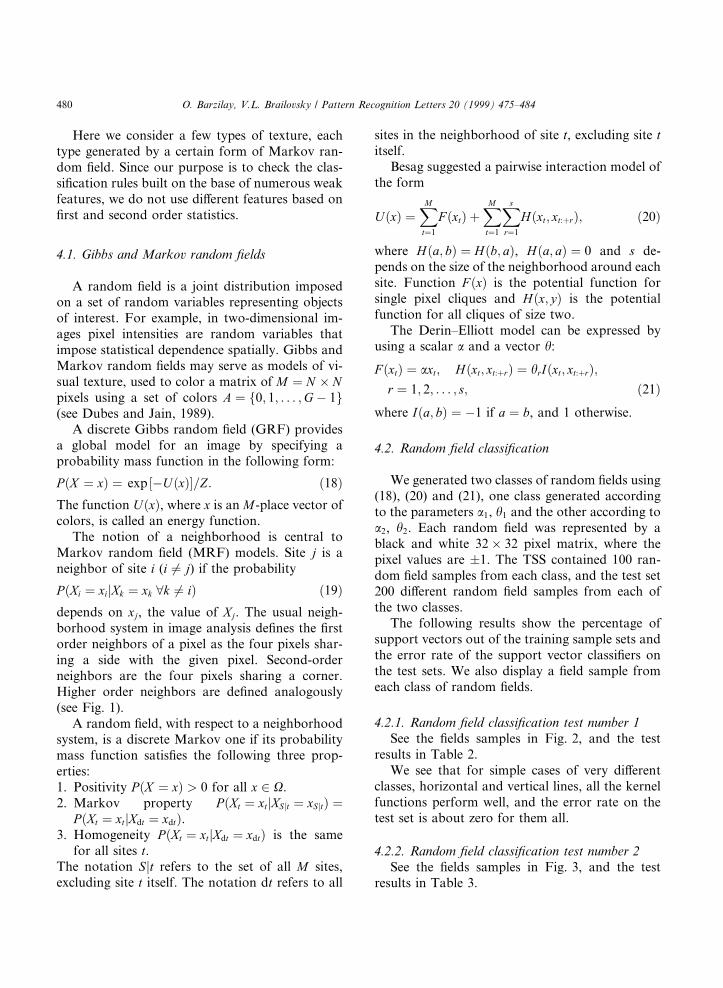
4.2.1. Random ®eld classi®cation test number 1See the ®elds samples in Fig. 2, and the test
results in Table 2.We see that for simple cases of very di�erent
classes, horizontal and vertical lines, all the kernelfunctions perform well, and the error rate on thetest set is about zero for them all.
4.2.2. Random ®eld classi®cation test number 2See the ®elds samples in Fig. 3, and the test
results in Table 3.
480 O. Barzilay, V.L. Brailovsky / Pattern Recognition Letters 20 (1999) 475±484
In this case of diagonal lines which is not muchmore di�cult than the previous case from a humanpoint of view, the regular kernel functions fail toperform any reasonable classi®cation while theneighborhood kernel function demonstrates ex-cellent performance.
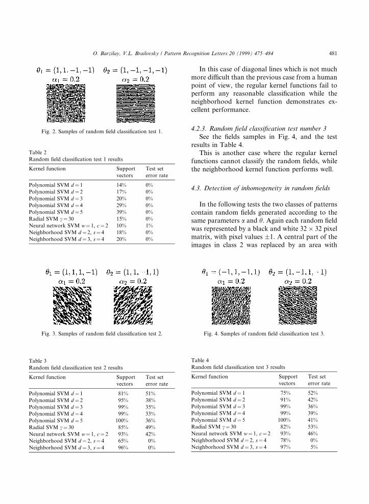
4.2.3. Random ®eld classi®cation test number 3See the ®elds samples in Fig. 4, and the test
results in Table 4.This is another case where the regular kernel
functions cannot classify the random ®elds, whilethe neighborhood kernel function performs well.
4.3. Detection of inhomogeneity in random ®elds
In the following tests the two classes of patternscontain random ®elds generated according to thesame parameters a and h. Again each random ®eldwas represented by a black and white 32� 32 pixelmatrix, with pixel values �1. A central part of theimages in class 2 was replaced by an area with
Fig. 4. Samples of random ®eld classi®cation test 3.
Table 4
Random ®eld classi®cation test 3 results
Kernel function Support
vectors
Test set
error rate
Polynomial SVM d � 1 75% 52%
Polynomial SVM d � 2 91% 42%
Polynomial SVM d � 3 99% 36%
Polynomial SVM d � 4 99% 39%
Polynomial SVM d � 5 100% 41%
Radial SVM c� 30 82% 53%
Neural network SVM w� 1, c� 2 93% 46%
Neighborhood SVM d � 2, s� 4 78% 0%
Neighborhood SVM d � 3, s� 4 97% 5%
Table 2
Random ®eld classi®cation test 1 results
Kernel function Support
vectors
Test set
error rate
Polynomial SVM d � 1 14% 0%
Polynomial SVM d � 2 17% 0%
Polynomial SVM d � 3 20% 0%
Polynomial SVM d � 4 29% 0%
Polynomial SVM d � 5 39% 0%
Radial SVM c� 30 15% 0%
Neural network SVM w� 1, c� 2 10% 1%
Neighborhood SVM d � 2, s� 4 18% 0%
Neighborhood SVM d � 3, s� 4 20% 0%
Table 3
Random ®eld classi®cation test 2 results
Kernel function Support
vectors
Test set
error rate
Polynomial SVM d � 1 81% 51%
Polynomial SVM d � 2 95% 38%
Polynomial SVM d � 3 99% 35%
Polynomial SVM d � 4 99% 33%
Polynomial SVM d � 5 100% 36%
Radial SVM c� 30 85% 49%
Neural network SVM w� 1, c� 2 93% 42%
Neighborhood SVM d � 2, s� 4 65% 0%
Neighborhood SVM d � 3, s� 4 96% 0%
Fig. 3. Samples of random ®eld classi®cation test 2.
Fig. 2. Samples of random ®eld classi®cation test 1.
O. Barzilay, V.L. Brailovsky / Pattern Recognition Letters 20 (1999) 475±484 481
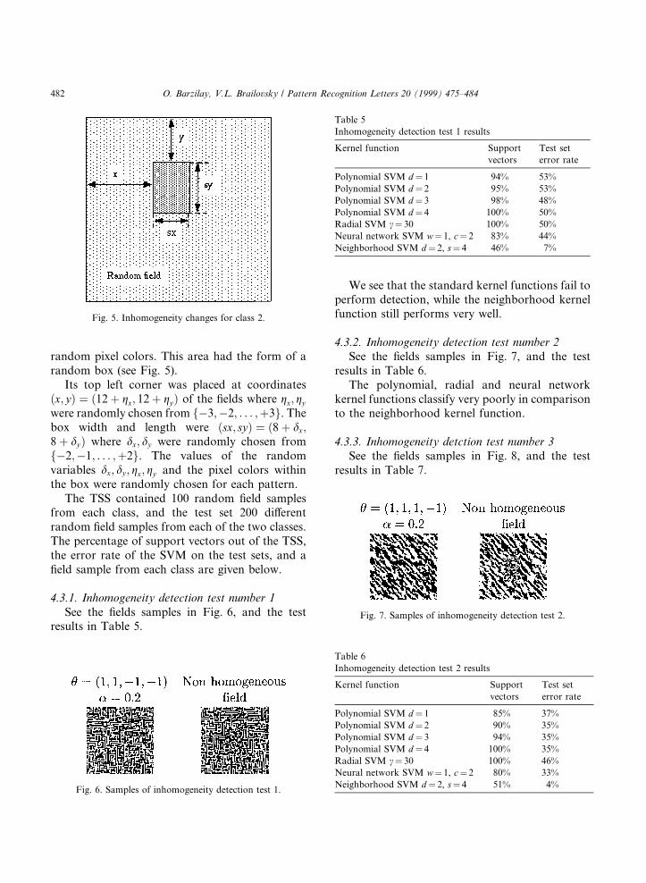
random pixel colors. This area had the form of arandom box (see Fig. 5).
Its top left corner was placed at coordinates�x; y� � �12� gx; 12� gy� of the ®elds where gx; gy
were randomly chosen from fÿ3;ÿ2; . . . ;�3g. Thebox width and length were �sx; sy� � �8� dx;8� dy� where dx; dy were randomly chosen fromfÿ2;ÿ1; . . . ;�2g. The values of the randomvariables dx; dy ; gx; gy and the pixel colors withinthe box were randomly chosen for each pattern.
The TSS contained 100 random ®eld samplesfrom each class, and the test set 200 di�erentrandom ®eld samples from each of the two classes.The percentage of support vectors out of the TSS,the error rate of the SVM on the test sets, and a®eld sample from each class are given below.
4.3.1. Inhomogeneity detection test number 1See the ®elds samples in Fig. 6, and the test
results in Table 5.
We see that the standard kernel functions fail toperform detection, while the neighborhood kernelfunction still performs very well.
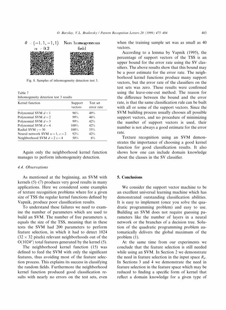
4.3.2. Inhomogeneity detection test number 2See the ®elds samples in Fig. 7, and the test
results in Table 6.The polynomial, radial and neural network
kernel functions classify very poorly in comparisonto the neighborhood kernel function.
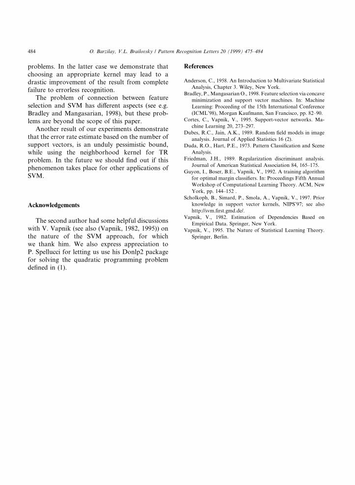
4.3.3. Inhomogeneity detction test number 3See the ®elds samples in Fig. 8, and the test
results in Table 7.
Fig. 5. Inhomogeneity changes for class 2.
Fig. 6. Samples of inhomogeneity detection test 1.
Table 5
Inhomogeneity detection test 1 results
Kernel function Support
vectors
Test set
error rate
Polynomial SVM d � 1 94% 53%
Polynomial SVM d � 2 95% 53%
Polynomial SVM d � 3 98% 48%
Polynomial SVM d � 4 100% 50%
Radial SVM c� 30 100% 50%
Neural network SVM w� 1, c� 2 83% 44%
Neighborhood SVM d � 2, s� 4 46% 7%
Fig. 7. Samples of inhomogeneity detection test 2.
Table 6
Inhomogeneity detection test 2 results
Kernel function Support
vectors
Test set
error rate
Polynomial SVM d � 1 85% 37%
Polynomial SVM d � 2 90% 35%
Polynomial SVM d � 3 94% 35%
Polynomial SVM d � 4 100% 35%
Radial SVM c� 30 100% 46%
Neural network SVM w� 1, c� 2 80% 33%
Neighborhood SVM d � 2, s� 4 51% 4%
482 O. Barzilay, V.L. Brailovsky / Pattern Recognition Letters 20 (1999) 475±484
Again only the neighborhood kernel functionmanages to perform inhomogeneity detection.
4.4. Observations
As mentioned at the beginning, an SVM withkernels (5)±(7) produces very good results in manyapplications. Here we considered some examplesof texture recognition problems where for a givensize of TSS the regular kernel functions de®ned byVapnik, produce poor classi®cation results.
To understand these failures we need to exam-ine the number of parameters which are used tobuild an SVM. The number of free parameters ai
equals the size of the TSS, meaning that in thesetests the SVM had 200 parameters to performfeature selection, in which it had to detect 1024(32� 32 pixels) relevant neighborhoods out of theO�1024d� total features generated by the kernel (5).
The neighborhood kernel function (15) wasde®ned to feed the SVM with only the signi®cantfeatures, thus avoiding most of the feature selec-tion process. This explains its success in classifyingthe random ®elds. Furthermore the neighborhoodkernel function produced good classi®cation re-sults with nearly no errors on the test sets, even
when the training sample set was as small as 40vectors.
According to a lemma by Vapnik (1995), thepercentage of support vectors of the TSS is anupper bound for the error rate using the SV clas-si®ers. The above results show that this bound maybe a poor estimate for the error rate. The neigh-borhood kernel functions produce many supportvectors, but the error rate of the classi®ers on thetest sets was zero. These results were con®rmedusing the leave-one-out method. The reason forthe di�erence between the bound and the errorrate, is that the same classi®cation rule can be builtwith all or some of the support vectors. Since theSVM building process usually chooses all possiblesupport vectors, and no procedure of minimizingthe number of support vectors is used, theirnumber is not always a good estimate for the errorrate.
Texture recognition using an SVM demon-strates the importance of choosing a good kernelfunction for good classi®cation results. It alsoshows how one can include domain knowledgeabout the classes in the SV classi®er.
5. Conclusions
We consider the support vector machine to bean excellent universal learning machine which hasdemonstrated outstanding classi®cation abilities.It is easy to implement (once you solve the qua-dratic programming problem) and easy to use.Building an SVM does not require guessing pa-rameters like the number of layers in a neuralnetwork or the branches of a decision tree. Solu-tion of the quadratic programming problem au-tomatically delivers the global maximum of theproblem (1).
At the same time from our experiments weconclude that the feature selection is still neededwhile using an SVM. In Section 2 we demonstratethe need in feature selection in the input space Rd .In Sections 3 and 4 we demonstrate the need infeature selection in the feature space which may bereduced to ®nding a speci®c form of kernel thatre¯ect a domain knowledge for a given type of
Table 7
Inhomogeneity detection test 3 results
Kernel function Support
vectors
Test set
error rate
Polynomial SVM d � 1 96% 49%
Polynomial SVM d � 2 99% 46%
Polynomial SVM d � 3 99% 42%
Polynomial SVM d � 4 100% 42%
Radial SVM c� 30 100% 55%
Neural network SVM w� 1, c� 2 92% 42%
Neighborhood SVM d � 2 s� 4 50% 6%
Fig. 8. Samples of inhomogeneity detection test 3.
O. Barzilay, V.L. Brailovsky / Pattern Recognition Letters 20 (1999) 475±484 483
problems. In the latter case we demonstrate thatchoosing an appropriate kernel may lead to adrastic improvement of the result from completefailure to errorless recognition.
The problem of connection between featureselection and SVM has di�erent aspects (see e.g.Bradley and Mangasarian, 1998), but these prob-lems are beyond the scope of this paper.
Another result of our experiments demonstratethat the error rate estimate based on the number ofsupport vectors, is an unduly pessimistic bound,while using the neighborhood kernel for TRproblem. In the future we should ®nd out if thisphenomenon takes place for other applications ofSVM.
Acknowledgements
The second author had some helpful discussionswith V. Vapnik (see also (Vapnik, 1982, 1995)) onthe nature of the SVM approach, for whichwe thank him. We also express appreciation toP. Spellucci for letting us use his Donlp2 packagefor solving the quadratic programming problemde®ned in (1).
References
Anderson, C., 1958. An Introduction to Multivariate Statistical
Analysis, Chapter 3. Wiley, New York.
Bradley, P., Mangasarian O., 1998. Feature selection via concave
minimization and support vector machines. In: Machine
Learning: Proceeding of the 15th International Conference
(ICML'98), Morgan Kaufmann, San Francisco, pp. 82±90.
Cortes, C., Vapnik, V., 1995. Support-vector networks. Ma-
chine Learning 20, 273±297.
Dubes, R.C., Jain, A.K., 1989. Random ®eld models in image
analysis. Journal of Applied Statistics 16 (2).
Duda, R.O., Hart, P.E., 1973. Pattern Classi®cation and Scene
Analysis.
Friedman, J.H., 1989. Regularization discriminant analysis.
Journal of American Statistical Association 84, 165±175.
Guyon, I., Boser, B.E., Vapnik, V., 1992. A training algorithm
for optimal margin classi®ers. In: Proceedings Fifth Annual
Workshop of Computational Learning Theory. ACM, New
York, pp. 144±152 .
Scholkoph, B., Simard, P., Smola, A., Vapnik, V., 1997. Prior
knowledge in support vector kernels, NIPS'97; see also
http://svm.®rst.gmd.de/.
Vapnik, V., 1982. Estimation of Dependencies Based on
Empirical Data. Springer, New York.
Vapnik, V., 1995. The Nature of Statistical Learning Theory.
Springer, Berlin.
484 O. Barzilay, V.L. Brailovsky / Pattern Recognition Letters 20 (1999) 475±484