Embed Size (px)
Citation preview
J Optim Theory ApplDOI 10.1007/s10957-013-0485-3
On Graph-Lagrangians of Hypergraphs ContainingDense Subgraphs
Qingsong Tang · Yuejian Peng · Xiangde Zhang ·Cheng Zhao
Received: 11 March 2013 / Accepted: 11 November 2013© Springer Science+Business Media New York 2013
Abstract Motzkin and Straus established a remarkable connection between the max-imum clique and the Graph-Lagrangian of a graph in (Can. J. Math. 17:533–540,1965). This connection and its extensions were successfully employed in optimiza-tion to provide heuristics for the maximum clique number in graphs. It is usefulin practice if similar results hold for hypergraphs. In this paper, we provide upperbounds on the Graph-Lagrangian of a hypergraph containing dense subgraphs whenthe number of edges of the hypergraph is in certain ranges. These results support apair of conjectures introduced by Peng and Zhao (Graphs Comb. 29:681–694, 2013)and extend a result of Talbot (Comb. Probab. Comput. 11:199–216, 2002).
Keywords Cliques of hypergraphs · Colex ordering · Graph-Lagrangians ofhypergraphs · Polynomial optimization
Communicated by Horst Martini.
Q. Tang · X. ZhangCollege of Sciences, Northeastern University, Shenyang, 110819, P.R. China
Q. Tange-mail: [email protected]
X. Zhange-mail: [email protected]
Q. Tang · C. Zhao (B)School of Mathematics, Jilin University, Changchun 130012, P.R. Chinae-mail: [email protected]
Y. PengCollege of Mathematics, Hunan University, Changchun 410082, P.R. Chinae-mail: [email protected]
C. ZhaoDepartment of Mathematics and Computer Science, Indiana State University, Terre Haute,IN, 47809 USA
J Optim Theory Appl
1 Introduction
In 1941, Turán [1] provided an answer to the following question: What is the maxi-mum number of edges in a graph with n vertices not containing a complete subgraphof order k, for a given k? This is the well-known Turán theorem. Later, in anotherclassical paper, Motzkin and Straus [2] provided a new proof of Turán theorem basedon the continuous characterization of the clique number of a graph using Graph-Lagrangians of graphs.
The Motzkin–Straus result basically says that the Graph-Lagrangian of a graphwhich is the maximum of a homogeneous quadratic multilinear function (determinedby the graph) over the standard simplex of the Euclidean space is connected tothe maximum clique number of this graph (the precise statement is given in Theo-rem 2.1). This result provides a solution to the optimization problem for a class of ho-mogeneous quadratic multilinear functions over the standard simplex of a Euclideanspace. The Motzkin–Straus result and its extension were successfully employed inoptimization to provide heuristics for the maximum clique problem [3–6]. It has beenalso generalized to vertex-weighted graphs [6] and edge-weighted graphs with appli-cations to pattern recognition in image analysis [3–9]. The Graph-Lagrangian of ahypergraph has been a useful tool in hypergraph extremal problems. For example,Sidorenko [10] and Frankl and Furedi [11] applied Graph-Lagrangians of hyper-graphs in finding Turán densities of hypergraphs. Frankl and Rödl [12] applied itin disproving Erdös long standing jumping constant conjecture. In most applications,we need an upper bound for the Graph-Lagrangian of a hypergraph.
An attempt to generalize the Motzkin–Straus theorem to hypergraphs is due to Sósand Straus [13]. Recently, in [14, 15] Rota Buló and Pelillo generalized the Motzkinand Straus’ result to r-graphs in some way using a continuous characterization ofmaximal cliques other than Graph-Lagrangians of hypergraphs. The obvious gen-eralization of Motzkin and Straus’ result to hypergraphs is false. In fact, there aremany examples of hypergraphs that do not achieve their Graph-Lagrangian on anyproper subhypergraph. We attempt to explore the relationship between the Graph-Lagrangian of a hypergraph and the order of its maximum cliques for hypergraphswhen the number of edges is in certain ranges though the obvious generalization ofMotzkin and Straus’ result to hypergraphs is false.
The results presented in Sects. 3 and 4 in this paper provide substantial evidencefor two conjectures in [16] and extend some known results in the literature [16,17]. The main results provide solutions to the optimization problem of a class ofhomogeneous multilinear functions over the standard simplex of the Euclidean space.The main results also give connections between a continuous optimization problemand the maximum clique problem of hypergraphs. Since practical problems such ascomputer vision and image analysis are related to the maximum clique problems, thistype of results opens a door to such practical applications. The results in this papercan be applied in estimating Graph-Lagrangians of some hypergraphs, for example,calculations involving estimating Graph-Lagrangians of several hypergraphs in [11]can be much simplified when applying the results in this paper.
The rest of the paper is organized as follows. In Sect. 2, we state a few definitions,problems, and preliminary results. In Sects. 3 and 4, we provide upper bounds on the
J Optim Theory Appl
Graph-Lagrangian of a hypergraph containing dense subgraphs when the number ofedges of the hypergraph is in a certain range. Then, as an application, using the mainresult in Sect. 3, we extend a result in [17] in Sect. 5. In Sect. 6, we give the proofsof some lemmas. Conclusions are given in Sect. 7.
2 Definitions and Preliminary Results
For a set V and a positive integer r we denote by V (r) the family of all r-subsetsof V . An r-uniform graph or r-graph G consists of a set V (G) of vertices anda set E(G) ⊆ V (G)(r) of edges. An edge e := {a1, a2, . . . , ar} will be simplydenoted by a1a2 . . . ar . An r-graph H is a subgraph of an r-graph G, denotedby H ⊆ G if V (H) ⊆ V (G) and E(H) ⊆ E(G). Let K
(r)t denote the complete
r-graph on t vertices, that is, the r-graph on t vertices containing all possibleedges. A complete r-graph on t vertices is also called a clique with order t . LetN be the set of all positive integers. For any integer n ∈ N, we denote the set{1,2,3, . . . , n} by [n]. Let [n](r) represent the complete r-uniform graph on the ver-tex set [n]. When r = 2, an r-uniform graph is a simple graph. When r ≥ 3, anr-graph is often called a hypergraph.
For an r-graph G = (V ,E) and i ∈ V , let Ei := {A ∈ V (r−1) : A ∪ {i} ∈ E}. Fora pair of vertices i, j ∈ V , let Eij := {B ∈ V (r−2) : B ∪ {i, j} ∈ E}. Let Ec
i := {A ∈V (r−1) : A ∪ {i} ∈ V (r)\E}, Ec
ij := {B ∈ V (r−2) : B ∪ {i, j} ∈ V (r)\E}, and Ei\j :=Ei ∩ Ec
j .
Definition 2.1 For an r-uniform graph G with the vertex set [n], edge set E(G),and a vector x := (x1, . . . , xn) ∈ R
n, we associate a homogeneous polynomial in n
variables, denoted by λ(G,x) as follows:
λ(G,x) :=∑
i1,i2,...,ir∈E(G)
xi1xi2 . . . xir .
Let S := {x := (x1, x2, . . . , xn) : ∑ni=1 xi = 1, xi ≥ 0 for i = 1,2, . . . , n}. Let λ(G)
represent the maximum of the above homogeneous multilinear polynomial of degreer over the standard simplex S. Precisely
λ(G) := max{λ(G,x) : x ∈ S
}.
The value xi is called the weight of the vertex i. A vector x := (x1, x2, . . . , xn) ∈R
n is called a feasible weighting for G iff x ∈ S. A vector y ∈ S is called an optimalweighting for G if λ(G,y) = λ(G). We call λ(G) the Graph-Lagrangian of G. Forsimplicity, we will write Graph-Lagrangian or G-Lagrangian in the rest of this paper.
The following fact is easily implied by Definition 2.1.
Fact 2.1 Let G1, G2 be r-uniform graphs and G1 ⊆ G2. Then λ(G1) ≤ λ(G2).
In [2], Motzkin and Straus provided the following simple expression for theG-Lagrangian of a 2-graph.
J Optim Theory Appl
Theorem 2.1 ([2, Theorem 1]) If G is a 2-graph with n vertices in which a largestclique has order t then λ(G) = λ(K
(2)t ) = 1
2 (1 − 1t). Furthermore, the vector x :=
(x1, x2, . . . , xn) given by xi := 1t
if i is a vertex in a fixed maximum clique and xi = 0otherwise is an optimal weighting.
This result provides a solution to the optimization problem of this type of ho-mogeneous quadratic functions over the standard simplex of an Euclidean space. Itis well-known that G-Lagrangians of hypergraphs have been proved to be a usefultool in hypergraph extremal problems, for example, they have been applied in findingTurán densities of hypergraphs in [10, 11, 18]. In order to explore the relationshipbetween the G-Lagrangian of a hypergraph and the order of its maximum cliquesfor hypergraphs when the number of edges is in certain ranges, the following twoconjectures are proposed in [17].
Conjecture 2.1 [16, Conjecture 1.3] Let m and t be positive integers satisfying(t−1r
) ≤ m ≤ (t−1r
) + (t−2r−1
). Let G be an r-graph with m edges and contain a clique
of order t − 1. Then λ(G) = λ([t − 1](r)).
Conjecture 2.2 [16, Conjecture 1.4] Let m and t be positive integers satisfying(t−1r
) ≤ m ≤ (t−1r
) + (t−2r−1
). Let G be an r-graph with m edges and contain no clique
of order t − 1. Then λ(G) < λ([t − 1](r)).
In [16], we proved that Conjecture 2.1 holds for r = 3.
Theorem 2.2 [16, Theorem 1.8] Let m and t be positive integers satisfying(t−1
3
) ≤m ≤ (
t−13
) + (t−2
2
). Let G be a 3-graph with m edges and contain a clique of order
t − 1. Then λ(G) = λ([t − 1](3)).
For distinct A,B ∈ N(r) we say that A is less than B in the colex ordering iff
max(A�B) ∈ B , where A�B := (A \ B) ∪ (B \ A). For example, we have 246 <
156 in N(3) since max({2,4,6}�{1,5,6}) ∈ {1,5,6}. In colex ordering, 123 < 124 <
134 < 234 < 125 < 135 < 235 < 145 < 245 < 345 < 126 < 136 < 236 < 146 <
246 < 346 < 156 < 256 < 356 < 456 < 127 < · · · . Note that the first(tr
)r-tuples in
the colex ordering of N(r) are the edges of [t](r).Let Cr,m denote the r-graph with m edges formed by taking the first m sets in the
colex ordering of N(r). The following result in [17] states that the value of λ(Cr,m)
can be easily figured out when m is in a certain range.
Lemma 2.1 [17, Lemma 2.4] For any integers m, t , and r satisfying(t−1r
) ≤ m ≤(t−1r
) + (t−2r−1
), we have λ(Cr,m) = λ([t − 1](r)).
Note that Conjectures 2.1 and 2.2 refine the following open conjecture of Frankland Füredi.
Conjecture 2.3 [11, Conjecture 4.1] The r-graph with m edges formed by taking thefirst m sets in the colex ordering of N(r) has the largest G-Lagrangian of all r-graphs
J Optim Theory Appl
with m edges. In particular, the r-graph with(tr
)edges and the largest G-Lagrangian
is [t](r).
Note that the upper bound(t−1r
) + (t−2r−1
)in Conjecture 2.1 is the best possible.
For example, if m = (t−1r
) + (t−2r−1
) + 1 then λ(Cr,m) > λ([t − 1](r)). To see this, take
x := (x1, . . . , xt ) ∈ S, where x1 = x2 = · · · = xt−2 = 1t−1 and xt−1 = xt = 1
2(t−1),
then λ(Cr,m) ≥ λ(Cr,m,x) > λ([t − 1](r)).In [17], Talbot proved the following:
Theorem 2.3 [17, Theorem 2.1] Let m and t be integers satisfying(t−1
3
) ≤ m ≤(t−1
3
) + (t−2
2
) − (t − 1). Then λ(G) ≤ λ([t − 1](3)).
Theorem 2.4 [17, Theorem 3.1] For any r ≥ 4 there exists constants γr and k0(r)
such that if m satisfies(
t − 1
r
)≤ m ≤
(t − 1
r
)+
(t − 2
r − 1
)− γr(t − 1)r−2
with t ≥ k0(r) and G is an r-graph on t vertices with m edges, then λ(G) ≤ λ([t −1](r)).
Note that, Theorems 2.3 and 2.4 in this paper are equivalent to Theorems 2.1 and3.1 in [18] after shifting t to t − 1.
Some evidence of Conjectures 2.1 and 2.2 can be found in [19, 20]. In particular,we proved
Theorem 2.5 [19, Theorem 1.10] (a) Let m and t be positive integers satisfying(
t − 1
r
)≤ m ≤
(t − 1
r
)+
(t − 2
r − 1
)− (2r−3 − 1)
((t − 2
r − 2
)− 1
).
Let G be an r-graph on t vertices with m edges and contain a clique of order t − 1.Then λ(G) = λ([t − 1](r)).
(b) Let m and t be positive integers satisfying(t−1
3
) ≤ m ≤ (t−1
3
)+ (t−2
2
)− (t − 2).Let G be a 3-graph with m edges and without containing a clique of order t − 1.Then λ(G) < λ([t − 1](3)).
In this paper, we provide upper bounds on the G-Lagrangian of a 3-graph,a 4-graph, and an r-graph, respectively, when the hypergraph contains dense sub-graphs and the number of edges of the hypergraph is in a certain range. These resultssupport Conjectures 2.1, 2.2 and extend Theorem 2.3.
We will impose one additional condition on any optimal weighting x := (x1, x2, . . . ,
xn) for an r-graph G:∣∣{i : xi > 0}∣∣ is minimal, i.e., if y is a feasible weighting for G satisfying∣∣{i : yi > 0}∣∣ <
∣∣{i : xi > 0}∣∣, then λ(G,y) < λ(G).(1)
J Optim Theory Appl
When the theory of Lagrange multipliers is applied to find the optimum of λ(G),subject to
∑ni=1 xi = 1, note that λ(Ei,x) corresponds to the partial derivative of
λ(G,x) with respect to xi . The following lemma gives some necessary conditions ofan optimal weighting of λ(G).
Lemma 2.2 [12, Theorem 2.1] Let G := (V ,E) be an r-graph on the vertex set [n]and x := (x1, x2, . . . , xn) be an optimal feasible weighting for G with k (≤ n) non-zero weights x1, x2, . . . , xk satisfying condition (1). Then for every {i, j} ∈ [k](2),
(a) λ(Ei,x) = λ(Ej ,x) = rλ(G),(b) there is an edge in E containing both i and j .
The following definition is also needed.
Definition 2.2 An r-graph G := (V ,E) on the vertex set [n] is left-compressed ifj1j2 . . . jr ∈ E implies i1i2 . . . ir ∈ E provided ip ≤ jp for every p,1 ≤ p ≤ r . Equiv-alently, an r-graph G := (V ,E) is left-compressed iff Ej\i = ∅ for any 1 ≤ i < j ≤ n.
Remark 2.1 (a) In Lemma 2.2, part (a) implies that
xjλ(Eij ,x) + λ(Ei\j ,x) = xiλ(Eij ,x) + λ(Ej\i ,x).
In particular, if G is left-compressed, then
(xi − xj )λ(Eij ,x) = λ(Ei\j ,x)
for any i, j satisfying 1 ≤ i < j ≤ k since Ej\i = ∅.(b) If G is left-compressed, then for any i, j satisfying 1 ≤ i < j ≤ k,
xi − xj = λ(Ei\j ,x)
λ(Eij ,x)(2)
holds. If G is left-compressed and Ei\j = ∅ for i, j satisfying 1 ≤ i < j ≤ k, thenxi = xj .
(c) By (2), if G is left-compressed, then an optimal feasible weighting x :=(x1, x2, . . . , xn) for G must satisfy
x1 ≥ x2 ≥ · · · ≥ xn ≥ 0. (3)
In the proofs of our results, we need to consider various left-compressed 3-graphson vertex set [t], which can be obtained from a Hessian diagram as follows.
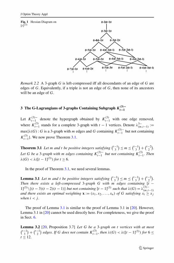
A triple i1i2i3 is called a descendant of a triple j1j2j3 iff is ≤ js for each 1 ≤ s ≤3, and i1 + i2 + i3 < j1 +j2 +j3. In this case, the triple j1j2j3 is called an ancestor ofi1i2i3. The triple i1i2i3 is called a direct descendant of j1j2j3 if i1i2i3 is a descendantof j1j2j3 and j1 + j2 + j3 = i1 + i2 + i3 + 1. We say that j1j2j3 has lower hierarchythan i1i2i3 if j1j2j3 is an ancestor of i1i2i3. This is a partial order on the set of alltriples. Figure 1 is a Hessian diagram on all triples on vertex set [t]. In this diagram,i1i2i3 and j1j2j3 are connected by an edge if i1i2i3 is a direct descendant of j1j2j3.
J Optim Theory Appl
Fig. 1 Hessian Diagram on[t](3)
Remark 2.2 A 3-graph G is left-compressed iff all descendants of an edge of G areedges of G. Equivalently, if a triple is not an edge of G, then none of its ancestorswill be an edge of G.
3 The G-Lagrangians of 3-graphs Containing Subgraph K(3)−t−1
Let K(3)−t−1 denote the hypergraph obtained by K
(3)t−1 with one edge removed,
where K(3)t−1 stands for a complete 3-graph with t − 1 vertices. Denote λ3−
(m,t−1) :=max{λ(G) : G is a 3-graph with m edges and G containing K
(3)−t−1 but not containing
K(3)t−1}. We now prove Theorem 3.1.
Theorem 3.1 Let m and t be positive integers satisfying(t−1
3
) ≤ m ≤ (t−1
3
) + (t−2
2
).
Let G be a 3-graph with m edges containing K(3)−t−1 but not containing K
(3)t−1. Then
λ(G) < λ([t − 1](3)) for t ≥ 6.
In the proof of Theorem 3.1, we need several lemmas.
Lemma 3.1 Let m and t be positive integers satisfying(t−1
3
) ≤ m ≤ (t−1
3
) + (t−2
2
).
Then there exists a left-compressed 3-graph G with m edges containing [t −1](3)\{(t − 3)(t − 2)(t − 1)} but not containing [t − 1](3) such that λ(G) = λ
(3)−(m,t−1)
and there exists an optimal weighting x := (x1, x2, . . . , xn) of G satisfying xi ≥ xj
when i < j .
The proof of Lemma 3.1 is similar to the proof of Lemma 3.1 in [20]. However,Lemma 3.1 in [20] cannot be used directly here. For completeness, we give the proofin Sect. 6.
Lemma 3.2 [20, Proposition 3.7] Let G be a 3-graph on t vertices with at most(t−1
3
) + (t−1
2
)edges. If G does not contain K
(3)t−1, then λ(G) < λ([t − 1](3)) for 6 ≤
t ≤ 12.
J Optim Theory Appl
Lemma 3.3 Let G be a left-compressed 3-graph containing [t − 1](3)\{(t − 3)(t −2)(t − 1)} but not containing [t − 1](3) with m edges such that λ(G) = λ3−
(m,t−1). Letx := (x1, x2, . . . , xn) be an optimal weighting of G and k be the number of positiveweights in x, then λ(G) < λ([t − 1])(3) or |[k − 1](3)\E| ≤ k − 2.
The proof of Lemma 3.3 is similar to Lemma 3.2 in [20]. However, Lemma 3.2 in[20] cannot be used directly here. For completeness, we give the details of the proofin Sect. 6.
Proof of Theorem 3.1 Let m and t be positive integers satisfying(t−1
3
) ≤ m ≤(t−1
3
) + (t−2
2
). Let G := (V ,E) be a 3-graph with m edges containing K
(3)−t−1 but not
containing K(3)t−1 such that λ(G) = λ3−
(m,t−1). Let x := (x1, x2, . . . , xn) be an optimal
weighting of G and k be the number of non-zero weights in x. By Lemma 3.1, wecan assume that G is left-compressed and contains [t − 1](3)\{(t − 3)(t − 2)(t − 1)}but does not contain [t − 1](3) and x1 ≥ x2 ≥ · · · ≥ xk > xk+1 = · · · = xn = 0. Sincex has only k positive weights, we can assume that G is on [k].
Now we proceed to show that λ(G) < λ([t − 1](3)). By Lemma 3.2, Theorem3.1 holds when t ≤ 12. Next we assume t ≥ 13. If λ(G) ≥ λ([t − 1](3)), then k ≥ t .Otherwise k ≤ t − 1, since G does not contain [t − 1](3), thus λ(G) < λ([t − 1](3)).
Since G is left-compressed and 1(k − 1)k ∈ E, then |[k − 2](2) ∩ Ek| ≥ 1. If k ≥t + 1, then applying Lemma 3.3, we have
m = |E| = ∣∣E ∩ [k − 1](3)∣∣ + ∣∣[k − 2](2) ∩ Ek
∣∣ + |E(k−1)k|
≥(
t
3
)− (t − 1) + 2
≥(
t − 1
3
)+
(t − 2
2
)+ 1, (4)
which contradicts the assumption that m ≤ (t−1
3
)+(t−2
2
). Recall that k ≥ t , so we have
k = t . Since λ3−(m,t−1) does not decrease as m increases, it is sufficient to show that
m = (t−1
3
)+ (t−1
2
). Let G′ := G∪{(t − 3)(t − 2)(t − 1)}\{1(t − 1)t}. If we can prove
that λ(G,x) < λ(G′,x), then since G′ contains [t − 1](3) and G′ has(t−1
3
) + (t−1
2
)
edges, we have λ(G′,x) ≤ λ(G′) = λ([t − 1](3)). Consequently, λ(G) < λ([t − 1]3).Now we show that λ(G,x) < λ(G′,x). Note that
λ(G′,x) − λ(G,x) = xt−3xt−2xt−1 − x1xt−1xt . (5)
By Remark 2.1(b), we have
x1 = xt−3 + λ(E1\(t−3),x)
λ(E1(t−3),x)(6)
and
xt−2 = xt + λ(E(t−2)\t ,x)
λ(E(t−2)t ,x). (7)
J Optim Theory Appl
Combining equations (5), (6) and (7), we get
λ(G′,x) − λ(G,x) = xt−3(xt + λ(E(t−2)\t ,x)
λ(E(t−2)t ,x))xt−1 − (xt−3 + λ(E1\(t−3),x)
λ(E1(t−3),x))xt−1xt
= λ(E(t−2)\t ,x)
λ(E(t−2)t ,x)xt−3xt−1 − λ(E1\(t−3),x)
λ(E1(t−3),x)xt−1xt . (8)
By Remark 2.1(b),
x1 = xt−2 + λ(E1\(t−2),x)
λ(E1(t−2),x)≤ xt−2 + xt−3xt−1 + (x2 + · · · + xt−3)xt
x2 + · · · + xt−3 + xt
< xt−2 + xt−1 + xt . (9)
Hence λ(E1(t−3),x)−λ(E(t−2)t ,x) ≥ xt−2 +xt−1 +xt −x1 > 0 and λ(E1(t−3),x) >
λ(E(t−2)t ,x). Clearly, xt−3 > xt since (t − 5)(t − 1) ∈ E(t−3)\t . Therefore, to showthat λ(G,x) < λ(G′,x), it is sufficient to show that
λ(E(t−2)\t ,x) ≥ λ(E1\(t−3),x). (10)
If (t −6)(t −1)t ∈ E, then all triples in [t](3) \{(t −3)(t −2)(t −1), ij t,where t −5 ≤ i < j ≤ t − 1} are edges in G since G is left-compressed. If E �= [t](3) \ {(t −3)(t − 2)(t − 1), ij t,where t − 5 ≤ i < j ≤ t − 1}, then m >
(t3
) − 11 ≥ (t−1
3
) +(t−2
2
)(recall that t ≥ 13), which is a contradiction. Therefore, either E = [t](3) \ {(t −
3)(t − 2)(t − 1), ij t,where t − 5 ≤ i < j ≤ t − 1} or (t − 6)(t − 1)t /∈ E.If E = [t](3) \ {(t − 3)(t − 2)(t − 1), ij t,where t − 5 ≤ i < j ≤ t − 1}, then
λ(E(t−2)\t ,x) = xt−5xt−1 + xt−5xt−3 + xt−5xt−4 + xt−4xt−3 + xt−4xt−1,
and
λ(E1\(t−3),x) = xt−2xt−1 + xt−5xt + xt−4xt + xt−2xt + xt−1xt .
Clearly, (10) holds in this case.If (t − 6)(t − 1)t /∈ E, then
λ(E(t−2)\t ,x) ≥ xt−3λ(E(t−3)(t−2) ∩ Ec
(t−3)t ,x) + xt−4xt−1 + xt−5xt−1 + xt−6xt−1
= xt−3λ(Ec
(t−3)t ,x) + xt−4xt−1 + xt−5xt−1 + xt−6xt−1
− xt−3xt−2 − xt−3xt−1
≥ xt−3λ(Ec
(t−3)t ,x) + xt−5xt−1 + xt−6xt−1 − xt−3xt−2
= xt−3(λ(Ec
(t−3)t ,x) − xt−2) + xt−5xt−1 + xt−6xt−1
and
λ(E1\(t−3),x) = xtλ(Ec
(t−3)t ,x) + xt−2xt−1
= xt
(λ(Ec
(t−3)t ,x) − xt−2
) + xt−2xt−1 + xt−2xt .
Clearly, (10) holds in this case.This completes the proof of Theorem 3.1. �
J Optim Theory Appl
Remark 3.1 Note that for t ≤ 5, the left-compressed 3-graph with(t−1
3
)+(t−1
2
)edges
always contains K(3)t−1. Combining Theorems 2.5 and 3.1, we have that, if G is a 3-
graph containing K(3)−t−1 with at most
(t−1
3
) + (t−1
2
)edges, then λ(G) ≤ λ([t − 1](3)).
Also, applying Theorem 3.1, we derive two easy corollaries that support Conjec-ture 2.2.
Corollary 3.1 Let m and t be positive integers satisfying(t−1
3
) ≤ m ≤ (t−1
3
) + (t−2
2
).
Let G := (V ,E) be a left-compressed 3-graph on the vertex set [t] with m edges andnot containing a clique of order t − 1. If |E(t−1)t | ≤ 3, then λ(G) < λ([t − 1](3)).
Proof Because λ3−(m,t−1)
doesn’t decrease as m increases, we can assume that m =(t−1
3
)+(t−2
2
). Since G := (V ,E) does not contain [t −1](3) and G is left-compressed,
(t − 3)(t − 2)(t − 1) /∈ E. If |E(t−1)t | = 1, then G must contain [t − 1](3). Therefore,|E(t−1)t | = 2 or 3.
If t ≤ 5, Theorem 3.1 clearly holds. Next, we assume t ≥ 6 and distinguish twocases.
Case 1. |E(t−1)t | = 2.Note that G is left-compressed, in view of Fig. 1,
E = [t](3) \ {3(t − 1)t,4(t − 1)t, . . . , (t − 2)(t − 1)t,
(t − 3)(t − 2)(t − 1), (t − 3)(t − 2)t}.
Case 2. |E(t−1)t | = 3.
In this case, since G is left-compressed, in view of Fig. 1, we only need to considerE = [t](3) \ {4(t − 1)t, . . . , (t − 2)(t − 1)t, (t − 3)(t − 2)(t − 1), (t − 3)(t − 2)t, (t −4)(t − 2)t}.
In both cases, left-compressed 3-graph G does not contain the edge (t − 3)(t −2)(t −1). Thus, the conditions in Theorem 3.1 are satisfied. Therefore, we are done. �
The next corollary states that if a 3-graph G contains a dense subgraph close tothe structure in C3,m, then we have λ(G) < λ([t − 1](3)).
Corollary 3.2 Let m and t be positive integers satisfying(t−1
3
) ≤ m ≤ (t−1
3
) + (t−2
2
).
Let G := (V ,E) be a left-compressed 3-graph on the vertex set [t] with m edgesand not containing a clique of size t − 1, and |E(G)�E(C3,m)| ≤ 6. Then, λ(G) <
λ([t − 1](3)).
Proof If m ≤ (t−1
3
) + (t−2
2
), then |E(t−1)t | ≤ 3, since otherwise |E(G)�E(C3,m)| >
6. Applying Corollary 3.2, we have λ(G) < λ([t − 1](3)). �
4 The G-Lagrangians of Hypergraphs Containing a Clique of Order t − 2 ort − 1
In this section, we prove the following:
J Optim Theory Appl
Theorem 4.1 Let m and t be positive integers satisfying(t−1
3
) ≤ m ≤ (t−1
3
)+ (t−2
2
)−t−2
2 . Let G be a 3-graph with m edges and G contain the maximum clique of ordert − 2. Then λ(G) < λ([t − 1](3)).
Theorem 4.2 Let m and t be positive integers satisfying(t−1r
) ≤ m ≤ (t−1r
)+ (t−2r−1
)−2r−2
((t−2r−2
) − 1). Let G be an r-graph on t vertices with m edges and with a clique
of order t − 2. Then λ(G) ≤ λ([t − 1](r)).
Theorem 4.3 Let m and t be positive integers satisfying(t−1
4
) ≤ m ≤ (t−1
4
)+ (� t−22 3
).
Let G be a 4-graph with m edges and a clique of order t − 1. Then λ(G) = λ([t −1](4)).
Here(t−1
4
) + (� t−22 3
)is not the best upper bound that we can obtain. This bound is
for simplicity of the proof.Denote λr
(m,p) := max{λ(G) : G is an r-graph with m edges and G contains amaximum clique of order p}.
Similar to the proof of Lemma 3.1 in [20], we can prove the following lemma. Wewill give the proof in Sect. 6.
Lemma 4.1 Let m and t be positive integers satisfying
(t − 1
3
)≤ m ≤
(t − 1
3
)+
(t − 2
2
)− t − 2
2.
Then there exists a left-compressed 3-graph G with m edges containing the maximumclique [t − 2](3) such that λ(G) = λ3
(m,t−2).
Similar to the proof of Lemma 3.2 in [20], we have the following lemma. Forcompleteness, we will give the proof in Sect. 6.
Lemma 4.2 Let G be a left-compressed 3-graph containing the maximum clique[t − 2](3) with m edges such that λ(G) = λ3
(m,t−2). Let x := (x1, x2, . . . , xn) be anoptimal weighting of G and k be the number of positive weights in x, then λ(G) <
λ([t − 1])(3) or |[k − 1](3)\E| ≤ k − 2.
We also need the following lemma whose proof is similar to Lemma 2.7 in [17]and Lemma 3.3 in [16]. We will give it in Sect. 6.
Lemma 4.3 Let m and t be positive integers satisfying(t−1
3
) ≤ m ≤ (t−1
3
) + (t−2
2
) −t−2
2 . Let G be a left-compressed 3-graph on the vertex set [t] and contain the maxi-mum clique [t −2](3) with m edges such that λ(G) = λ3
(m,t−2). Assume b := |E(t−1)t |,then λ(G) < λ([t − 1](3)) or
∣∣[t − 2](2)\Et
∣∣ ≤ b.
J Optim Theory Appl
Proof of Theorem 4.1 Let m and t be positive integers satisfying(t−1
3
) ≤ m ≤ (t−1
3
)+(t−2
2
) − t−22 . Clearly, we can assume that t ≥ 5. Let G := (V ,E) be a 3-graph with
m edges containing a maximum clique of order t − 2 such that λ(G) = λ3(m,t−2).
Let x := (x1, x2, . . . , xn) be an optimal weighting of G and k be the number of non-zero weights in x. By Lemma 4.1, we can assume that G is left-compressed with themaximum clique [t − 2](3) and x1 ≥ x2 ≥ · · · ≥ xk > xk+1 = · · · = xn = 0. Since xhas only k positive weights, we can assume that G is on [k].
Now we proceed to show that λ(G) < λ([t − 1](3)). If λ(G) ≥ λ([t − 1](3)), thenk ≥ t . Otherwise k ≤ t − 1, since G does not contain [t − 1](3), then λ(G) < λ([t −1](3)). By Lemma 2.2(a), k−1 and k appear in some common edge e ∈ E. Recall thatE is left-compressed, so 1(k − 1)k ∈ E. Define b := max{i : i(k − 1)k ∈ E}. BecauseE is left-compressed, Ei\j = ∅ for 1 ≤ i < j ≤ b. Hence, by Remark 2.1(a), we havex1 = x2 = · · · = xb . Clearly, b ≤ k − 5.
Since G is left-compressed and 1(k − 1)k ∈ E, then |[k − 2](2) ∩ Ek| ≥ 1. Soapplying Lemma 4.2, similar to (4), we have k = t .
Since k = t , we can assume that G is on [t]. By Remark 2.1(b), we have
x1 = xt−3 + λ(E1\(t−3),x)
λ(E1(t−3),x).
Recall that G contains a clique order of t − 2, we have
λ(E1\(t−3),x) = xt−1λ(Ec
(t−3)(t−1),x) + xtλ
(Ec
(t−3)t ,x) − xt−1xt .
Hence
x1 < xt−3 + xt−1λ(Ec(t−3)(t−1),x) + xtλ(Ec
(t−3)t ,x)
λ(E1(t−3),x).
Since for i �= t − 1, t − 2, t − 3, i ∈ Ec(t−3)t implies that i(t − 3) ∈ [t − 2](2)\Et
and i ∈ Ec(t−2)t implies that i(t − 2) ∈ [t − 2](2)\Et , t − 1 ∈ Ec
(t−3)t , t − 1 ∈ Ec(t−2)t ,
and t − 2 ∈ Ec(t−3)t , t − 3 ∈ Ec
(t−2)t and (t − 2)(t − 3) ∈ [t − 2](2)\Et , applyingLemma 4.3, then
∣∣Ec(t−3)t
∣∣ + ∣∣Ec(t−2)t
∣∣ ≤ ∣∣[t − 2](2)\Et
∣∣ + 3 ≤ b + 3.
Note that b ≤ t − 5 and∣∣Ec
(t−3)t
∣∣ ≤ ∣∣Ec(t−2)t
∣∣.
So∣∣Ec
(t−3)t
∣∣ ≤ b + 3
2≤ t − 2
2.
Since G is left-compressed, then
∣∣Ec(t−3)(t−1)
∣∣ ≤ ∣∣Ec(t−3)t
∣∣ ≤ t − 2
2.
J Optim Theory Appl
So
x1 < xt−3 + xt−1λ(Ec(t−3)(t−1),x) + xtλ(Ec
(t−3)t ,x)
λ(E1(t−3),x)
≤ xt−3 + xt−1t−2
2λ(E1(t−3),x)
t−2 + xtt−2
2λ(E1(t−3),x)
t−2
λ(E1(t−3),x)
≤ 2xt−3.
This implies
2xt−3xt−2xt−1 − x1xt−1xt > 0.
Let C := [t − 1](3)\E be all triples containing t − 1 not in E,
E′ := E ∪C∖{(
b−⌊ |C|
2
⌋+1
)(t −1)t,
(b−
⌊ |C|2
⌋+2
)(t −1)t, . . . , b(t −1)t
}
and G′ := ([t](3),E′). Then
λ(G′, x) − λ(G,x) = λ(C,x) −⌊ |C|
2
⌋x1xt−1xt
≥ |C|xt−3xt−2xt−1 −⌊ |C|
2
⌋x1xt−1xt
≥ |C|2
(2xt−3xt−2xt−1 − x1xt−1xt ) > 0.
So λ(G,x) < λ(G′, x). Because
|E′| = |E| + |C| −⌊ |C|
2
⌋≤ |E| + |C|
2+ 1
≤(
t − 1
3
)+
(t − 2
2
)− t − 2
2+ t − 4
2+ 1
=(
t − 1
3
)+
(t − 2
2
)
and G′ contains a clique of order t − 1, we have λ(G′, x) ≤ λ(G′) = λ([t − 1](3)) byTheorem 2.2. Hence λ(G,x) < λ(G′, x) ≤ λ([t − 1](3)). This proves Theorem 4.1. �
The following lemma implies that we only need to consider left-compressedr-graphs when Theorem 4.2 is proved. The proof is given in Sect. 6.
Lemma 4.4 Let m and t be positive integers satisfying
(t − 1
r
)≤ m ≤
(t
r
)− 1.
J Optim Theory Appl
Then there exists a left-compressed G with m edges containing the clique [t − 2](r)such that λ(G) = λr
(m,t−2) and there exists an optimal weighting x := (x1, x2, . . . , xn)
of G satisfying xi ≥ xj when i < j .
We also need the following in the proof of Theorems 4.2 and 4.3
Lemma 4.5 [19, Theorem 3.4] Let r ≥ 3 and t ≥ r + 2 be positive integers. Let G bea left-compressed r-graph on t vertices satisfying |[t − 2](r−1)\Et | ≥ 2r−3|E(t−1)t |.Then
(a) If G contains [t − 1](r), then λ(G) = λ([t − 1](r)),(b) If G does not contain [t − 1](r), then λ(G) < λ([t − 1](r)).
Proof of Theorem 4.2 Let m and t be positive integers satisfying(t−1r
) ≤ m ≤ (t−1r
)+(t−2r−1
) − 2r−2((t−2r−2
) − 1). Let G be an r-graph with m edges and t vertices witha clique order of t − 2. By Lemma 4.4, we can assume G is left-compressed. ByLemma 4.5, it is sufficient to show that |[t − 2](r−1)\Et | ≥ 2r−3|E(t−1)t |. If not,then |[t − 2](r−1)\Et | < 2r−3|E(t−1)t | and |[t − 2](r−1)\Et−1| ≤ |[t − 2](r−1)\Et | <2r−3|E(t−1)t |. Since G contains the clique [t − 2](r),
m =(
t − 2
r
)+ 2
(t − 2
r − 1
)− ∣∣[t − 2](r−1)\Et
∣∣ − ∣∣[t − 2](r−1)\Et−1∣∣ + ∣∣E(t−1)t
∣∣
>
(t − 1
r
)+
(t − 2
r − 1
)−
(t − 2
r − 2
)− (2r−2 − 1)
∣∣E(t−1)t
∣∣ + 1
≥(
t − 1
r
)+
(t − 2
r − 1
)− 2r−2
((t − 2
r − 2
)− 1
);
since |E(t−1)t | ≤(t−2r−2
) − 1, this is a contradiction. Note that if |E(t−1)t | =(t−2r−2
)then
E = [t](r) since G is left-compressed and m = (tr
), which results in a contradiction,
too. This proves Theorem 4.2. �
Remark 4.1 Lemma 4.5(b) and Theorem 4.2 imply that if m and t are positive inte-gers satisfying
(t − 1
r
)≤ m ≤
(t − 1
r
)+
(t − 2
r − 1
)− 2r−2
((t − 2
r − 2
)− 1
)
and G is a r-graph on t vertices with m edges and with a maximum clique of ordert − 2. Then
λ(G) < λ([t − 1](r)).
Proof of Theorem 4.3 Let m and t be positive integers satisfying(t−1
4
) ≤ m ≤ (t−1
4
)+(� t−2
2 3
). Let G be a 4-graph with m edges and a clique of order t −1. Since it contains
a clique of order t − 1, without loss of generality, we may assume that it contains
J Optim Theory Appl
[t − 1](4). Since G contains [t − 1](4), we have λ(G) ≥ λ([t − 1](4)). Next we provethat λ(G) ≤ λ([t − 1](4)).
Let x := (x1, x2, . . . , xn) be an optimal weighting of G and k be the number ofnon-zero weights in x. If k ≤ t − 1, clearly λ(G) ≤ λ([t − 1](4)). Assume that k ≥t . Recall that
(t−1
4
) ≤ m ≤ (t−1
4
) + (� t−22 3
)and G contains [t − 1](4), hence |Ek| ≤
(� t−22 3
). By Fact 2.1, Lemma 2.2(a) and Theorem 2.3, we have
λ(G,x) = 1
4λ(Ek,x) ≤ 1
4
(� t−22 3
)(1
� t−22
)3
≤ (t − 4)(t − 6)
24(t − 2)2<
(t − 2)(t − 3)(t − 4)
24(t − 1)3= λ
([t − 1](4)). �
Remark 4.2 Also note that Theorem 3.1, Theorem 4.1, and Remark 4.1 provide fur-ther evidence for Conjecture 2.2. Theorem 4.3 provide further evidence for Conjec-ture 2.1.
5 Remarks
Frankl and Füredi [11] asked the following question: Given r ≥ 3 and m ∈ N howlarge can the G-Lagrangian of an r-graph with m edges be? Conjecture 2.3 proposesa solution to the question mentioned above.
Denote
λrm := max{λ(G) : G is an r-graph with m edges}.
The following lemma implies that we only need to consider left-compressed r-graphswhen Conjecture 2.3 is explored.
Lemma 5.1 [17, Lemma 2.3] There exists a left-compressed r-graph G with m edgessuch that
λ(G) = λrm.
We extend Theorem 2.3 in Theorem 5.1 which is a corollary of Theorem 3.1.
Theorem 5.1 Let m and t be positive integers satisfying(t−1
3
) ≤ m ≤ (t−1
3
)+ (t−2
2
)−(t − 4). Then Conjecture 2.3 is true for r = 3 and this value of m.
Proof Let x := (x1, x2, . . . , xn) be an optimal weighting for G and k be the numberof positive weights in x. We can assume that G is left-compressed by Lemma 5.1.So x1 ≥ x2 ≥ · · · ≥ xk > xk+1 = · · · = xn = 0 by Remark 2.1(c). Since x has only k
positive weights, we can assume that G is on vertex set [k].Now we proceed to show that λ(G) ≤ λ([t − 1](3)). If λ(G) > λ([t − 1](3)), then
k ≥ t since otherwise k ≤ t − 1 and then λ(G) ≤ λ([t − 1](3)). Next we apply thefollowing lemma.
J Optim Theory Appl
Lemma 5.2 [17, Lemma 2.5] Let m be a positive integer. Let G be a left-compressed3-graph with m edges such that λ(G) = λ3
m. Let x := (x1, x2, . . . , xn) be an optimalweighting for G and k be the number of non-zero weights in x, then
∣∣[k − 1](3)\E∣∣ ≤ k − 2.
So similar to (4), we have k = t . Next we need the following lemma whose prooffollows the lines of Lemma 2.5 in [17]. For completeness, we give the proof in Sect. 6.
Lemma 5.3 Let G be a left-compressed 3-graph on the vertex set [t] with m edgeswhere
(t − 1
3
)≤ m ≤
(t − 1
3
)+
(t − 2
2
),
and λ(G) = λ3m. Let x := (x1, x2, . . . , xt ) be an optimal weighting for G. Then
∣∣[t − 1](3)\E∣∣ ≤ t − 3 or λ(G) ≤ λ([t − 1](3)
).
Assuming Lemma 5.3 holds, we continue the proof of Theorem 5.1. If λ(G) >
λ([t −1](3)), then |[t −1](3)\E| ≤ t −3 by Lemma 5.3, we add any |[t −1](3) \E|−1triples in [t − 1](3) \ E to E and let the new 3-graph be G′. Then G′ contains K
(3)−t−1 ,
the number of edges in G′ is at most(t−1
3
)+ (t−2
2
)and λ(G′) ≥ λ(G). Applying The-
orem 2.5 and Theorem 3.1, λ(G′) ≤ λ([t − 1](3)). Therefore, λ(G) ≤ λ([t − 1](3)) =λ(C3,m) by Lemma 2.1. This completes the proof of Theorem 5.1. �
6 Proofs of Some Lemmas
Proof techniques of lemmas in this section follow from proof techniques of somelemmas in [17, 19, 20]. As mentioned earlier, lemmas in those papers cannot beapplied directly to situations in this paper. For completeness, we give the proofs ofthese lemmas in this section.
Proof of Lemma 3.1 Let G be a 3-graph on the vertex set [n] with m edges containingK
(3)−t−1 but not containing K
(3)t−1 such that λ(G) = λ3−
(m,t−1). We call such a 3-graph G
an extremal 3-graph for m and t − 1. Let x := (x1, x2, . . . , xn) be an optimal weight-ing of G. We can assume that xi ≥ xj when i < j since otherwise we can just relabelthe vertices of G and obtain another extremal 3-graph for m and t −1 with an optimalweighting x := (x1, x2, . . . , xn) satisfying xi ≥ xj when i < j . Next we obtain a new3-graph G′ from G by performing the following:
1. If (t −3)(t −2)(t −1) ∈ E(G), then there is at least one triple in [t −1](3) \E(G),we replace (t − 3)(t − 2)(t − 1) by this triple;
2. If an edge in G has a descendant other than (t − 3)(t − 2)(t − 1) that is not inE(G), then replace this edge by a descendant other than (t − 3)(t − 2)(t − 1) withthe lowest hierarchy. Repeat this until there is no such an edge.
J Optim Theory Appl
Then G′ satisfies the following properties:
1. The number of edges in G′ is the same as the number of edges in G;2. λ(G) = λ(G,x) ≤ λ(G′,x) ≤ λ(G′);3. (t − 3)(t − 2)(t − 1) /∈ E(G′);4. [t − 1](3)\{(t − 3)(t − 2)(t − 1)} ∈ E(G′);5. For any edge in E(G′), all its descendants other than (t − 3)(t − 2)(t − 1) will be
in E(G′).
If G′ is not left-compressed, then there is an ancestor uvw of (t − 3)(t − 2)(t − 1)
such that uvw ∈ E(G′). We claim that uvw must be (t − 3)(t − 2)t . If uvw is not(t −3)(t −2)t , then since all descendants other than (t −3)(t −2)(t −1) of uvw willbe in E(G′), then all descendants of (t − 3)(t − 1)t (other than (t − 3)(t − 2)(t − 1))or all descendants of (t − 3)(t − 2)(t + 1) (other than (t − 3)(t − 2)(t − 1)) will be inE(G′). So all triples in [t − 1](3) \ {(t − 3)(t − 2)(t − 1)}, all triples in the form of ij t
(where ij ∈ [t − 2](2)), and all triples in the form of ij (t + 1) (where ij ∈ [t − 2](2))or all triples in the form of i(t − 1)l, 1 ≤ i ≤ t − 3 will be in E(G′), then
m ≥(
t − 1
3
)− 1 +
(t − 2
2
)+ (t − 3) >
(t − 1
3
)+
(t − 2
2
),
which is a contradiction. So uvw must be (t − 3)(t − 2)t . Since m ≤ (t−1
3
) + (t−2
2
)
and all the descendants other than (t − 3)(t − 2)(t − 1) of an edge in G′ will be anedge in G′, then there are two possibilities.
Case 1 E(G′) = ([t − 1](3) \ {(t − 1)(t − 2)(t − 3)}) ∪ {ij t, ij ∈ [t − 2](2)}∪ {12(t + 1)}.
Case 2 E(G′) = ([t − 1](3) \ {(t − 1)(t − 2)(t − 3)}) ∪ {ij t, ij ∈ [t − 2](2)}.Let y := (y1, y2, . . . , yn) be an optimal weighting of G′, where n = t + 1 or n = t .
We claim that if Case 1 happens, then yt = yt+1 = 0, since E(t−1)t = Et(t+1) = ∅(by Lemma 2.2). If Case 2 happens, then yt = 0 since E(t−1)t = ∅ (by Lemma 2.2).Hence we can assume that G is left-compressed. �
Proof of Lemma 3.3 Since G contains the clique of [t − 1](3)\{(t − 3)(t − 2)(t − 1)},it is true for k ≤ t . Next we assume that k ≥ t + 1.
Since G is left-compressed, 1(k −1)k ∈ E. Let b := max{i : i(k −1)k ∈ E}. SinceE is left-compressed, then Ei := {1, . . . , i − 1, i + 1, . . . , k}(2), for 1 ≤ i ≤ b, andEi\j = ∅ for 1 ≤ i < j ≤ b. Hence, by Remark 2.1(a), we have x1 = x2 = · · · = xb .
We define a new feasible weighting y for G as follows. Let yi = xi for i �= k−1, k,yk−1 = xk−1 + xk and yk = 0.
By Lemma 2.2(a), λ(Ek−1,x) = λ(Ek,x), so
λ(G,y) − λ(G,x) = xk
(λ(Ek−1,x) − xkλ(Ek(k−1),x)
)
− xk
(λ(Ek,x) − xk−1λ(Ek(k−1),x)
) − xk−1xkλ(Ek(k−1),x)
= xk
(λ(Ek−1,x) − λ(Ek,x)
) − x2k
b∑
i=1
xi
= −bx1x2k . (11)
J Optim Theory Appl
Since yk = 0 we may remove all edges containing k from E to form a new 3-graphG := ([k],E) with |E| := |E| − |Ek| and λ(G,y) = λ(G,y). We will show that ifLemma 3.3 fails to hold then there exists a set of edges F ⊂ [k − 1](3) \ E satisfying
λ(F,y) > bx1x2k (12)
and
|F | ≤ |Ek|. (13)
Then, using (11), (12), and (13), the 3-graph G′ := ([k],E′), where E′ := E ∪ F ,satisfies |E′| ≤ |E| and
λ(G′,y) = λ(G,y) + λ(F,y)
> λ(G,y) + bx1x2k
= λ(G,x).
Hence λ(G′) > λ(G). Note that G′ still contains [t − 1](3)\{(t − 3)(t − 2)(t − 1)}since G′ contains all edges in E ∩ [k − 1](3) ⊇ E ∩ [t − 1](3). If G′ does not containsa clique of size t − 1, note that G′ still contains [t − 1](3)\{(t − 3)(t − 2)(t − 1)}, itcontradicts the fact that λ(G) = λ3−
(m,t−1). If G′ contains a clique of size t − 1, then,
by Theorem 2.5, λ(G′) = λ([t − 1](3)), and consequently λ(G′) < λ([t − 1](3)).We must now construct the set of edges F satisfying (12) and (13). Applying
Remark 2.1(a) by taking i = 1, j = k − 1, we have
x1 = xk−1 + λ(E1\(k−1),x)
λ(E1(k−1),x).
Let C := [k − 2](2) \ Ek−1. Then λ(E1\(k−1),x) = xk
∑k−2i=b+1 xi + λ(C,x). Ap-
plying this and multiplying bx2k to the above equation (note that λ(E1(k−1),x) =∑k
i=2,i �=k−1 xi ), we have
bx1x2k = bxk−1x
2k + bx3
k
∑k−2i=b+1 xi
∑ki=2,i �=k−1 xi
+ bx2k λ(C,x)
∑ki=2,i �=k−1 xi
.
Since x1 ≥ x2 ≥ · · · ≥ xk ,
bx1x2k ≤ bxk−1x
2k
(1 + k − (b + 2)
k − 3
)+ bxkλ(C,x)
k − 2. (14)
Define α := � b|C|k−2 � and β := �b(1 + k−(b+2)
k−3 )�. Note that �b(1 + k−(b+2)k−3 )� ≤ k − 2
since b ≤ k −2. So β ≤ k −2. Let the set F1 ⊂ [k −1](3) \E consist of the α heaviestedges in [k − 1](3) \ E containing the vertex k − 1 (note that |[k − 2](2) \ Ek−1| =|C| ≥ α). Recalling that yk−1 = xk−1 + xk , we have
λ(F1,y) ≥ bxkλ(C,x)
k − 2+ αxk−1x
2k .
J Optim Theory Appl
So using (14)
λ(F1,y) − bx1x2k ≥ xk−1x
2k (α − β). (15)
We now distinguish two cases.
Case 1. α > β .
In this case, λ(F1,y) − bxk−1x2k > 0 so defining F := F1 shows (12). We need
to check that |F | ≤ |Ek|. Since E is left-compressed, then [b](2) ∪ {1, . . . , b} × {b +1, . . . , k − 1} ⊂ Ek . Hence
|Ek| ≥ b[b − 1 + 2(k − 1 − b)]2
≥ b(k − 1)
2(16)
since b ≤ k − 2. Recall that |F | = α = � b|C|k−2 �. Since C ⊂ [k − 2](2), we have |C| ≤(
k−22
). So using (16), we obtain
|F | ≤⌈
b(k − 3)
2
⌉≤ b(k − 1)
2≤ |Ek|.
So both (12) and (13) are satisfied.
Case 2. α ≤ β .
Suppose that Lemma 3.3 fails to hold. So |[k − 1](3) \ E| ≥ k − 1 ≥ β + 1 (recallthat β ≤ k − 2). Let F2 consist of any β + 1 − α edges in [k − 1](3) \ (E ∪ F1) anddefine F := F1 ∪ F2. Then since λ(F2,y) ≥ (β + 1 − α)x3
k−1 and using (15),
λ(F,y) − bxk−1x2k = λ(F1,y) − bxk−1x
2k + λ(F2,y)
≥ (β + 1 − α)x3k−1 − xk−1x
2k (β − α) > 0.
So (12) is satisfied. What remains is to check that |F | ≤ |Ek|. In fact,
|F | = β + 1 ≤ k − 1 ≤ b(k − 1)
2≤ |Ek|
when b ≥ 2. If b = 1, then
|F | = β + 1 = 3 ≤ k − 2 = b[b − 1 + 2(k − 1 − b)]2
≤ |Ek|
since k ≥ t ≥ 5. �
Proof of Lemma 4.1 Let G be a 3-graph on the vertex set [n] with m edges containinga maximal clique of order t − 2 such that λ(G) = λ3
(m,t−2). We call such a G anextremal 3-graph for m and t − 2. Let x := (x1, x2, . . . , xn) be an optimal weightingof G. We can assume that xi ≥ xj when i < j since otherwise we can just relabel thevertices of G and obtain another extremal 3-graph for m and t − 2 with an optimalweighting x := (x1, x2, . . . , xn) satisfying xi ≥ xj when i < j . Next we obtain a new3-graph G′ from G by performing the following:
J Optim Theory Appl
1. If (t − 3)(t − 2)(t − 1) ∈ E(G), then there is at least one triple in [t − 1](3)\E(G),we replace (t − 3)(t − 2)(t − 1) by this triple;
2. If an edge in G has a descendant other than (t − 3)(t − 2)(t − 1) that is not inE(G), then replace this edge by a descendant other than (t − 3)(t − 2)(t − 1) withthe lowest hierarchy. Repeat this until there is no such edge.
Then G′ satisfies the following:
1. The number of edges in G′ is the same as the number of edges in G;2. G contains the clique [t − 2](3);3. λ(G) = λ(G,x) ≤ λ(G′,x) ≤ λ(G′);4. (t − 3)(t − 2)(t − 1) /∈ E(G′);5. For any edge in E(G), all its descendants other than (t − 3)(t − 2)(t − 1) will be
in E(G′).
If G′ is not left-compressed, then there is an ancestor uvw of (t − 3)(t − 2)(t − 1)
such that uvw ∈ G′ and all the descendant of uvw other than uvw are in G′. Hence
E(G′) ⊇ ([t − 1](3)\{(t − 3)(t − 2)(t − 1)}) ∪ {
ij t, ij ∈ [t − 2](2)}
and
m ≥(
t − 1
3
)− 1 +
(t − 2
2
)>
(t − 1
3
)+
(t − 2
2
)− t − 2
2,
which is a contradiction. Hence G′ is left-compressed. �
Proof of Lemma 4.2 Since G contains the clique of [t − 2](3), it is true for k ≤ t − 1.Assume that k ≥ t .
Since G is left-compressed, 1(k −1)k ∈ E. Let b := max{i : i(k −1)k ∈ E}. SinceE is left-compressed, Ei = {1, . . . , i −1, i +1, . . . , k}(2), for 1 ≤ i ≤ b, and Ei\j = ∅for 1 ≤ i < j ≤ b. Hence, by Remark 2.1(a), we have x1 = x2 = · · · = xb.
We define a new feasible weighting y for G as follows. Let yi := xi for i �= k−1, k,yk−1 := xk−1 + xk and yk := 0.
By Lemma 2.2(a), λ(Ek−1,x) = λ(Ek,x), so
λ(G,y) − λ(G,x) = xk
(λ(Ek−1,x) − xkλ(Ek(k−1),x)
)
− xk
(λ(Ek,x) − xk−1λ(Ek(k−1),x)
) − xk−1xkλ(Ek(k−1),x)
= xk
(λ(Ek−1,x) − λ(Ek,x)
) − x2k
b∑
i=1
xi
= −bx1x2k . (17)
Since yk = 0, we may remove all edges containing k from E to form a new 3-graphG := ([k],E) with |E| := |E| − |Ek| and λ(G,y) = λ(G,y). We will show that ifLemma 4.2 fails to hold then there exists a set of edges F ⊂ [k − 1](3) \ E satisfying
λ(F,y) > bx1x2k (18)
J Optim Theory Appl
and
|F | ≤ |Ek|. (19)
Then, using (17), (18), and (19), the 3-graph G′ := ([k],E′), where E′ := E ∪ F ,satisfies |E′| ≤ |E| and
λ(G′,y) = λ(G,y) + λ(F,y)
> λ(G,y) + bx1x2k
= λ(G,x).
Hence λ(G′) > λ(G). Note that G′ still contains the clique [t −2](3) since G′ containsall edges in E ∩[k −1](3) ⊃ [t −2](3). If G′ does not contains a clique of size t −1, itcontradicts to λ(G) = λ3
(m,t−2). If G′ contains a clique of size t − 1, then by Theorem
2.2 λ(G′) = λ([t − 1](3)), and consequently λ(G′) < λ([t − 1](3)).We must now construct the set of edges F satisfying (18) and (19). Applying
Remark 2.1(a) by taking i = 1, j = k − 1, we have
x1 = xk−1 + λ(E1\(k−1),x)
λ(E1(k−1),x).
Let C := [k − 2](2) \ Ek−1. Then λ(E1\(k−1),x) = xk
∑k−2i=b+1 xi + λ(C,x). Ap-
plying this and multiplying bx2k to the above equation (note that λ(E1(k−1),x) =∑k
i=2,i �=k−1 xi ), we have
bx1x2k = bxk−1x
2k + bx3
k
∑k−2i=b+1 xi
∑ki=2,i �=k−1 xi
+ bx2k λ(C,x)
∑ki=2,i �=k−1 xi
.
Since x1 ≥ x2 ≥ · · · ≥ xk ,
bx1x2k ≤ bxk−1x
2k
(1 + k − (b + 2)
k − 3
)+ bxkλ(C,x)
k − 2. (20)
Define α := � b|C|k−2 � and β := �b(1 + k−(b+2)
k−3 )�. Note that �b(1 + k−(b+2)k−3 )� ≤ k − 2
since b ≤ k −2. So β ≤ k −2. Let the set F1 ⊂ [k −1](3) \E consist of the α heaviestedges in [k − 1](3) \ E containing the vertex k − 1 (note that |[k − 2](2) \ Ek−1| =|C| ≥ α). Recalling that yk−1 = xk−1 + xk , we have
λ(F1,y) ≥ bxkλ(C,x)
k − 2+ αxk−1x
2k .
So using (20),
λ(F1,y) − bx1x2k ≥ xk−1x
2k (α − β). (21)
We now distinguish two cases.
J Optim Theory Appl
Case 1. α > β .
In this case, λ(F1,y) − bxk−1x2k > 0 so defining F := F1 shows (18). We need
to check that |F | ≤ |Ek|. Since E is left-compressed, then [b](2) ∪ {1, . . . , b} × {b +1, . . . , k − 1} ⊂ Ek . Hence
|Ek| ≥ b[b − 1 + 2(k − 1 − b)]2
≥ b(k − 1)
2(22)
since b ≤ k − 2. Recall that |F | = α = � b|C|k−2 �. Since C ⊂ [k − 2](2), we have |C| ≤(
k−22
). So using (20), we obtain
|F | ≤⌈
b(k − 3)
2
⌉≤ b(k − 1)
2≤ |Ek|.
So both (18) and (19) are satisfied.
Case 2. α ≤ β .
Suppose that Lemma 4.2 fails to hold. So |[k − 1](3) \ E| ≥ k − 1 ≥ β + 1 (recallthat β ≤ k − 2). Let F2 consist of any β + 1 − α edges in [k − 1](3) \ (E ∪ F1) anddefine F := F1 ∪ F2. Then since λ(F2,y) ≥ (β + 1 − α)x3
k−1 and using (21),
λ(F,y) − bxk−1x2k = λ(F1,y) − bxk−1x
2k + λ(F2,y)
≥ (β + 1 − α)x3k−1 − xk−1x
2k (β − α) > 0.
So (18) is satisfied. What remains is to check that |F | ≤ |Ek|. In fact,
|F | = β + 1 ≤ k − 1 ≤ b(k − 1)
2≤ |Ek|
when b ≥ 2. If b = 1, then applying (21),
|F | = β + 1 = 3 ≤ k − 2 = b[b − 1 + 2(k − 1 − b)]2
≤ |Ek|
since k ≥ t ≥ 5. �
Proof of Lemma 4.3 Let b := max{i : i(t −1)t ∈ E}. Since E is left-compressed, thenEi = {1, . . . , i − 1, i + 1, . . . , t}(2), for 1 ≤ i ≤ b and Ei\j = ∅ for 1 ≤ i < j ≤ b.
Hence, by Remark 2.1(a), we have x1 = x2 = · · · = xb . Consider a new weightingfor G, y := (y1, y2, . . . , yt ) given by yi := xi for i �= t − 1, t , yt−1 := 0 and yt :=xt−1 + xt . By Lemma 2.2(a), λ(Et−1,x) = λ(Et ,x), so
λ(G,y) − λ(G,x) = xt−1(λ(Et ,x) − λ(Et−1,x)
) − x2t−1
b∑
i=1
xi = −bx1x2t−1. (23)
Since yt−1 = 0, we may remove all edges containing t − 1 from E to form a new3-graph G := ([t],E) with |E| := |E| − |Et−1| and λ(G,y) = λ(G,y).
J Optim Theory Appl
If |[t −2](2)\Et | > b, we will show that there exists a set of edges F ⊂ {1, . . . , t −2, t}(3) \ E satisfying
λ(F,y) > bx1x2t−1. (24)
Then using (23) and (24), the 3-graph G′ := ([t],E′), where E′ := E ∪F , satisfiesλ(G′,y) > λ(G). Since y has only t − 1 positive weights, then λ(G′,y) ≤ λ([t −1](3)), and consequently
λ(G) < λ([t − 1](3)
).
We must now construct the set of edges F . Since G is left-compressed, applyingRemark 2.1(a) by taking i = 1, j = t , we get
x1 = xt + λ(E1\t ,x)
λ(E1t ,x).
Let D := [t − 2](2) \Et . Then λ(E1\t ,x) = xt−1∑t−2
i=b+1 xi +λ(D,x). Applying this
and multiplying bx2t−1 to the above equation (note that λ(E1t ,x) = ∑t−1
i=2 xi ), we have
bx1x2t−1 = bxtx
2t−1 + bx3
t−1
∑t−2i=b+1 xi
∑t−1i=2 xi
+ bx2t−1λ(D,x)∑t−1
i=2 xi
.
Let c :=∑t−2
i=b+1 xi∑t−1i=2 xi
and d := bxt−1∑t−1i=2 xi
. Then
bx1x2t−1 = bxtx
2t−1 + bcx3
t−1 + dxt−1λ(D,x). (25)
Let F consist of those edges in {1, . . . , t − 2, t}(3) \ E containing the vertex t . Then
λ(F,y) = (xt−1 + xl)λ(D,x). (26)
Since |[t − 2](2)\Et | > b,
λ(D,x) > bx2t−1. (27)
Applying equations (25), (26), and (27), we get
λ(F,y) − bx1x2t−1 = (xt−1 + xt )λ(D,x) − bxtx
2t−1 − bcx3
t−1 − dxt−1λ(D,x)
= [(1 − d)xt−1 + xt
]λ(D,x) − bxtx
2t−1 − bcx3
t−1
>[(1 − d)xt−1 + xt
]bx2
t−1 − bxtx2t−1 − bcx3
t−1
= bx3t−1(1 − d − c) ≥ 0
since
c + d =∑t−2
i=b+1 xi + bxt−1∑t−1
i=2 xi
≤ 1.
J Optim Theory Appl
Let G′ := ([t],E ∪ F), then λ(G′,y) = λ(G,y) + λ(F,y) = λ(G,x) − bx1x2t−1 +
λ(F,y) > λ(G,x). On the other hand, since y has only t − 1 positive weights, thenλ(G′,y) < λ([t − 1](3)). �
Proof of Lemma 4.4 Let m and t be positive integers satisfying(t−1r
) ≤ m ≤ (tr
) − 1.Let G := (V ,E) be an r-graph on vertex set V := [n] with m edges containing aclique of size t − 2 such that λ(G) = λr
(m,t−2). We call such a G an extremal r-graph
for m and t − 2. Let x := (x1, x2, . . . , xn) be an optimal weighting of G. We canassume that xi ≥ xj when i < j since otherwise we can just relabel the verticesof G and obtain another extremal r-graph for m and t − 2 with an optimal x :=(x1, x2, . . . , xn) satisfying xi ≥ xj when i < j . If G is not left-compressed, then thereis an edge whose ancestor is not an edge. Replace all those edges by its availableancestor with the highest hierarchy, then we get a left-compressed r-graph G′ whichcontains the clique [t − 2](r) and λ(G′,x) ≥ λ(G,x). �
Proof of Lemma 5.3 Let b := max{i : i(t −1)t ∈ E}. Since E is left-compressed, thenEi = {1, . . . , i − 1, i + 1, . . . , t}(2), for 1 ≤ i ≤ b, and Ei\j = ∅ for 1 ≤ i < j ≤ b.
Hence, by Remark 2.1(a), we have x1 = x2 = · · · = xb . We define a new feasibleweighting y for G as follows. Let yi := xi for i �= t − 1, t , yt−1 := xt−1 + xt andyt := 0.
By Lemma 2.2(a), λ(Et−1,x) = λ(Et ,x), so
λ(G,y) − λ(G,x) = xt
(λ(Et−1,x) − xtλ(Et(t−1),x)
)
− xt
(λ(Et ,x) − xt−1λ(E(t−1)t ,x)
) − xt−1xtλ(E(t−1)t ,x)
= xt
(λ(Et−1,x) − λ(Et ,x)
) − x2t
b∑
i=1
xi
= −bx1x2t . (28)
Since yt = 0, we may remove all edges containing t from E to form a new 3-graphG := ([t],E) with |E| := |E| − |Et | and λ(G,y) = λ(G,y).
We will show that if |[t − 1](3) \ E| ≥ t − 2 then there exists a set of edges F ⊂[t − 1](3) \ E satisfying
λ(F,y) ≥ bx1x2t , (29)
Then, using (28), (29), the 3-graph G′ := ([t],E′), where E′ := E ∪ F , satisfies
λ(G′,y) = λ(G,y) + λ(F,y)
≥ λ(G,y) + bx1x2t
= λ(G,x).
Since y has only t − 1 positive weights, λ(G′) ≤ λ([t − 1](3)), and consequently,λ(G) ≤ λ([t − 1](3)).
J Optim Theory Appl
We must now construct the set of edges F satisfying (29). Applying Remark 2.1(a)by taking i = 1, j = t − 1, we have
x1 = xt−1 + λ(E1\(t−1),x)
λ(E1(t−1),x).
Let C := [t − 2](2) \ Et−1. Then λ(E1\(t−1),x) = xt
∑t−2i=b+1 xi + λ(C,x). Ap-
plying this and multiplying bx2t to the above equation (note that λ(E1(t−1),x) =∑t
i=2,i �=t−1 xi ), we have
bx1x2t = bxt−1x
2t + bx3
t
∑t−2i=b+1 xi∑t
i=2,i �=t−1 xi
+ bx2t λ(C,x)
∑ti=2,i �=t−1 xi
.
Since x1 ≥ x2 ≥ · · · ≥ xt ,
bx1x2t ≤ bxt−1x
2t
(1 + t − (b + 2)
t − 3
)+ bxtλ(C,x)
t − 2. (30)
Define α := � b|C|t−2 � and β := �b(1 + t−(b+2)
t−3 )�. Note that since b ≤ t − 2. So β ≤t − 2. Let the set F1 ⊂ [t − 1](3) \ E consist of the α heaviest edges in [t − 1](3) \ E
containing the vertex t − 1 (note that |[t − 2](2) \ Et−1| = |C| ≥ α). Recalling thatyt−1 = xt−1 + xt , we have
λ(F1,y) ≥ bxtλ(C,x)
t − 2+ αxt−1x
2t .
So using (30),
λ(F1,y) − bx1x2t ≥ xt−1x
2t (α − β). (31)
If α > β , then λ(F1,y) − bxt−1x2t > 0. So defining F := F1 shows (29).
Assume α ≤ β . Suppose that |[t −1](3)\E| ≥ t −2. So |[t −1](3) \E| ≥ t −2 ≥ β
(recall that β ≤ t − 2). Let F2 consist of any β − α edges in [t − 1](3) \ (E ∪ F1) anddefine F := F1 ∪ F2. Then since λ(F2,y) ≥ (β − α)x3
t−1 and using (30),
λ(F,y) − bxt−1x2t = λ(F1,y) − bxt−1x
2t + λ(F2,y)
≥ (β − α)x3t−1 − xt−1x
2t (β − α) ≥ 0.
This proves Lemma 5.3. �
7 Conclusions
At this moment, we are not able to extend the arguments in this paper to verify Con-jectures 2.1, 2.2, and 2.3 for more general cases. When r ≥ 4, the computation ismore complex. If there is some technique to overcome this difficulty, then the ideaused in proving Theorem 3.1 can be used to improve our results much further.
J Optim Theory Appl
Acknowledgements We thank two anonymous referees and the editor for helpful and insightful com-ments.
We also thank Professor Franco Giannessi for suggesting the terminology ‘Graph-Lagrangian’.This research is partially supported by National Natural Science Foundation of China (No. 11271116).
References
1. Turán, P.: On an extremal problem in graph theory. Mat. Fiz. Lapok 48, 436–452 (1941)2. Motzkin, T.S., Straus, E.G.: Maxima for graphs and a new proof of a theorem of Turán. Can. J. Math.
17, 533–540 (1965)3. Bomze, I.M.: Evolution towards the maximum clique. J. Glob. Optim. 10, 143–164 (1997)4. Budinich, M.: Exact bounds on the order of the maximum clique of a graph. Discrete Appl. Math.
127, 535–543 (2003)5. Busygin, S.: A new trust region technique for the maximum weight clique problem. Discrete Appl.
Math. 154, 2080–2096 (2006)6. Gibbons, L.E., Hearn, D.W., Pardalos, P.M., Ramana, M.V.: Continuous characterizations of the max-
imum clique problem. Math. Oper. Res. 22, 754–768 (1997)7. Pavan, M., Pelillo, M.: Generalizing the Motzkin–Straus theorem to edge-weighted graphs, with appli-
cations to image segmentation. In: Rangarajan, A., Figueiredo Mário, A.T., Zerubia, J. (eds.) LectureNotes in Computer Science, vol. 2683, pp. 485–500. Spring, New York (2003)
8. Pardalos, P.M., Phillips, A.: A global optimization approach for solving the maximum clique problem.Int. J. Comput. Math. 33, 209–216 (1990)
9. Buló, S.R., Torsello, A., Pelillo, M.: A continuous-based approach for partial clique enumeration. In:Escolano, F., Vento, M. (eds.) Lecture Notes in Computer Science, vol. 4538, pp. 61–70. Spring, NewYork (2007)
10. Sidorenko, A.F.: Solution of a problem of Bollobás on 4-graphs. Mat. Zametki 41, 433–455 (1987)11. Frankl, P., Füredi, Z.: Extremal problems whose solutions are the blow-ups of the small Witt-designs.
J. Comb. Theory, Ser. A 52, 129–147 (1989)12. Frankl, P., Rödl, V.: Hypergraphs do not jump. Combinatorica 4, 149–159 (1984)13. Sós, V.T., Straus, E.G.: Extremals of functions on graphs with applications to graphs and hypergraphs.
J. Comb. Theory, Ser. A 32, 246–257 (1982)14. Bulò, S.R., Pelillo, M.: A continuous characterization of maximal cliques in k-uniform hypergraphs.
In: Maniezzo, V., Battiti, R., Watson, J.P. (eds.) Lecture Notes in Computer Science, vol. 5313, pp.220–233. Spring, New York (2008)
15. Bulò, S.R., Pelillo, M.: A generalization of the Motzkin–Straus theorem to hypergraphs. Optim. Lett.3, 287–295 (2009)
16. Peng, Y., Zhao, C.: A Motzkin–Straus type result for 3-uniform hypergraphs. Graphs Comb. 29, 681–694 (2013)
17. Talbot, J.M.: Lagrangians of hypergraphs. Comb. Probab. Comput. 11, 199–216 (2002)18. Mubayi, D.: A hypergraph extension of Turán’s theorem. J. Comb. Theory, Ser. B 96, 122–134 (2006)19. Peng, Y., Tang, Q., Zhao, C.: On Lagrangians of r-uniform Hypergraphs. J. Comb. Optim. (2013).
doi:10.1007/s10878-013-9671-320. Peng, Y., Zhu, H., Zheng, Y., Zhao, C.: On Cliques and Lagrangians of 3-uniform hypergraphs.
Preprint (2012). arXiv:1211.6508