Queueing Syst (2012) 71:199–220DOI 10.1007/s11134-012-9276-z

On the distribution of typical shortest-path lengthsin connected random geometric graphs

D. Neuhäuser · C. Hirsch · C. Gloaguen ·V. Schmidt

Received: 25 March 2011 / Published online: 2 February 2012© Springer Science+Business Media, LLC 2012

Abstract Stationary point processes in R2 with two different types of points, say

H and L, are considered where the points are located on the edge set G of a ran-dom geometric graph, which is assumed to be stationary and connected. Examplesinclude the classical Poisson–Voronoi tessellation with bounded and convex cells,aggregate Voronoi tessellations induced by two (or more) independent Poisson pro-cesses whose cells can be nonconvex, and so-called β-skeletons being subgraphsof Poisson–Delaunay triangulations. The length of the shortest path along G froma point of type H to its closest neighbor of type L is investigated. Two differentmeanings of “closeness” are considered: either with respect to the Euclidean distance(e-closeness) or in a graph-theoretic sense, i.e., along the edges of G (g-closeness).For both scenarios, comparability and monotonicity properties of the correspondingtypical shortest-path lengths Ce∗ and Cg∗ are analyzed. Furthermore, extending theresults which have recently been derived for Ce∗, we show that the distribution ofCg∗ converges to simple parametric limit distributions if the edge set G becomesunboundedly sparse or dense, i.e., a scaling factor κ converges to zero and infinity,respectively.

Keywords Point process · Aggregate tessellation · β-skeleton · Shortest path · Palmmark distribution · Stochastic monotonicity · Scaling limit

Mathematics Subject Classification (2000) Primary 60D05 · Secondary 60G55 ·60F99 · 90B15

D. Neuhäuser · C. Hirsch · V. Schmidt (�)Institute of Stochastics, Ulm University, 89069 Ulm, Germanye-mail: volker.schmidt@uni-ulm.de

C. GloaguenOrange Labs, 38-40, rue du Général Leclerc, 92794 Issy-les-Moulineaux, Francee-mail: catherine.gloaguen@orange-ftgroup.com

200 Queueing Syst (2012) 71:199–220

1 Introduction

In this paper we extend results on distributional properties of typical shortest-pathlengths in spatial stochastic network models which have recently been derived in[8, 17, 18]. More precisely, we consider stochastic models for networks with twohierarchy levels, i.e., there are network components of two different kinds: high-levelcomponents (HLC) and low-level components (LLC). The locations of both HLC andLLC are represented by points on the edge set G of a random geometric graph [13] inR

2 which is assumed to be stationary and connected. It is clear that this is fulfilled forthe edge set of stationary tessellations with convex cells (see, for example [14, 15]).But, for instance, also for so-called aggregate tessellations [2, 16] and β-skeletons[1, 10] induced by homogeneous Poisson processes.

Each LLC is assumed to be connected to its closest HLC, where two differentmeanings of “closeness” are considered: either with respect to the Euclidean dis-tance (e-closeness) or in a graph-theoretic sense, i.e., along the edges of the graph(g-closeness). In applications, e.g., to telecommunication networks, the edges of therandom geometric graph can represent the underlying infrastructure, for instance, aninner-city street system. In this case, one is especially interested in the distributionof shortest-path lengths along the edge set between the LLC and their closest HLC,which is an important performance characteristic in cost and risk analysis as well asin strategic planning of wired telecommunication.

In [8, 17, 18], we associated with each HLC a certain subset of R2 which is called

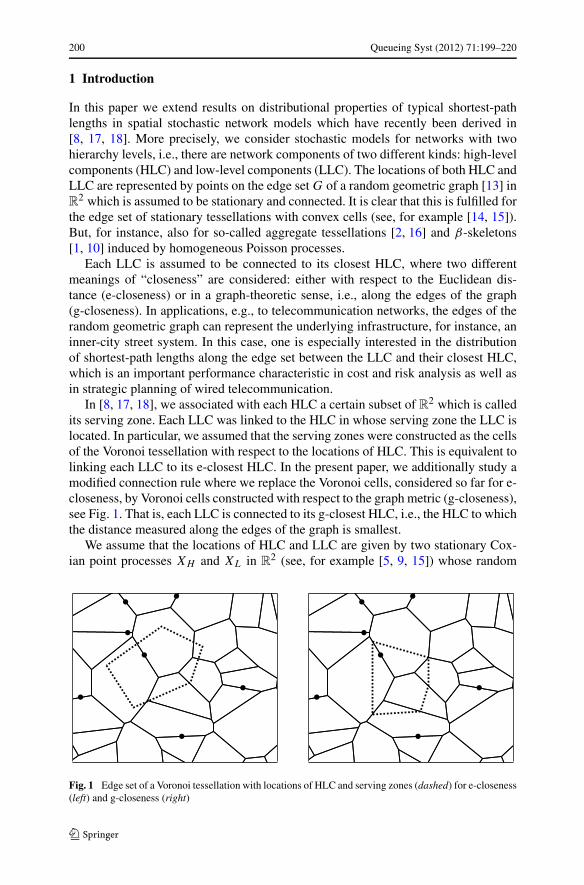
its serving zone. Each LLC was linked to the HLC in whose serving zone the LLC islocated. In particular, we assumed that the serving zones were constructed as the cellsof the Voronoi tessellation with respect to the locations of HLC. This is equivalent tolinking each LLC to its e-closest HLC. In the present paper, we additionally study amodified connection rule where we replace the Voronoi cells, considered so far for e-closeness, by Voronoi cells constructed with respect to the graph metric (g-closeness),see Fig. 1. That is, each LLC is connected to its g-closest HLC, i.e., the HLC to whichthe distance measured along the edges of the graph is smallest.

We assume that the locations of HLC and LLC are given by two stationary Cox-ian point processes XH and XL in R

2 (see, for example [5, 9, 15]) whose random

Fig. 1 Edge set of a Voronoi tessellation with locations of HLC and serving zones (dashed) for e-closeness(left) and g-closeness (right)

Queueing Syst (2012) 71:199–220 201

intensity measures are concentrated on G. In particular, we assume that (i) XH andXL are conditionally independent given G and (ii) their random intensity measuresare proportional to the one-dimensional Hausdorff measure on G, with some (linear)intensities λ�,λ

′� > 0 for XH and XL, respectively.

In this case, one is especially interested in the distributions of the typical shortest-path lengths Ce∗ and Cg∗ along the edge set between the points of XL and theire-closest resp. g-closest neighbors in XH . Note that even for simple examples of sta-tionary and fully connected edge sets G in R

2, the distributions of Ce∗ and Cg∗ arenot known analytically. However, asymptotic results can be derived if the edge setG becomes unboundedly sparse or dense. In particular, under some additional condi-tions, it can be shown that the distributions of Ce∗ and Cg∗ converge to exponentialand Weibull distributions, respectively, which do not depend on the selected closenessscenario. Furthermore, it can be shown that the distribution of Cg∗ does not dependon λ′

� and, for g-closeness, that it decreases stochastically in λ�, i.e., the values of thedistribution function of Cg∗ increase pointwise if λ� increases. Although increasingthe linear intensity λ� of XH certainly decreases the size of the typical serving zonefor both e-closeness and g-closeness, it seems to be an open problem whether in thecase of e-closeness the distribution of Ce∗ decreases stochastically in λ�. However,our numerical experiments clearly indicate that this should be true; see Sect. 6. Onthe other hand, it can be shown that Cg∗ under g-closeness is stochastically smallerthan Ce∗ under e-closeness.

The paper is organized as follows. In Sect. 2 we describe the hierarchical net-work model investigated in the present paper. Examples of random geometric graphs,which are stationary and connected, are discussed in Sect. 3. Then, Sect. 4 deals withcomparability and monotonicity properties of the distributions of typical shortest-pathlengths Ce∗ and Cg∗. Afterwards, in Sect. 5, we investigate the asymptotic behaviorof these distributions for unboundedly sparse and dense networks, respectively. InSect. 6, we present some numerical results. Finally, Sect. 7 concludes the paper andgives an outlook to future research.

2 Stochastic modeling of hierarchical networks

To begin with, we give a short description of the hierarchical network model inves-tigated in the present paper. In particular, we briefly introduce some fundamentalclasses of models from stochastic geometry which we are using in order to constructthe network model. The reader, who is interested in further details, is referred to well-known monographs, see, for example [5, 9, 15] for random (marked) point processesand, in particular, Coxian point processes, [13] for random geometric graphs, [14, 15]for random tessellations, and [11, 14] for general random closed sets.

2.1 Marked point processes

First we recall some basic notions regarding marked point processes in R2. Let B2

denote the family of Borel sets of R2, and let M be a Polish space with its Borel

σ -algebra BM. Furthermore, for any n ≥ 1, let Xn : Ω → R2 and Mn : Ω → M be

202 Queueing Syst (2012) 71:199–220

random variables defined on some probability space (Ω, A,P) such that #{n : Xn ∈B} < ∞ with probability 1 for each bounded B ∈ B2. Then, X = {(Xn,Mn),n ≥ 1}is said to be a marked point process with mark space M.

Note that we can regard X as a random element of (NM, NM), where NM is thefamily of all counting measures on B2 ⊗ BM which are simple and locally finite inthe first component, and NM is the usual σ -algebra on NM. We thus can regard a(marked) point process X as a random counting measure, i.e., X = {X(B × E),B ∈B2,E ∈ BM}, where

X(B × E) = #{n : Xn ∈ B,Mn ∈ E}.For x ∈ R

2, we define the shift tx : NM → NM by txX = tx{(Xn,Mn)} = {(Xn −x,Mn)}. Assume now that X = {(Xn,Mn)} is stationary with intensity λ ∈ (0,∞),

i.e., Xd= txX for each x ∈ R

2, whered= means equality of distributions; λ = E#{n :

Xn ∈ [0,1)2}. Then the Palm mark distribution PoX : BM → [0,1] of X is given by

PoX(E) = 1

λE#

{n : Xn ∈ [0,1)2,Mn ∈ E

}, E ∈ BM. (1)

A random variable M∗ distributed according to PoX is called the typical mark of X.

In the following, two jointly stationary marked point processes X(1) ={(X(1)

n ,M(1)n )} and X(2) = {(X(2)

n ,M(2)n )} with intensities λ1 and λ2 and mark spaces

M1 and M2, respectively, will be considered as a random element Y = (X(1),X(2))

of the product space NM1,M2 = NM1 × NM2 . The Palm distribution P∗X(i) of Y with

respect to the ith component, i = 1,2, is then defined on NM1 ⊗ NM2 ⊗ BMiby

P∗X(i) (A × E) = 1

λi

E#{n : X(i)

n ∈ [0,1)2,M(i)n ∈ E, t

X(i)n

Y ∈ A}, (2)

where A ∈ NM1 ⊗ NM2 and E ∈ BMi. Note that the Palm mark distribution P

oX(i) of

X(i) can be obtained from P∗X(i) as a marginal distribution.

2.2 Random geometric graphs

The edge set of a random geometric graph can be described by an F -valued randomvariable G : Ω → F such that P(G ∈ S) = 1, where F denotes the family of allclosed subsets of R

2, and S ⊂ F is the family of all locally finite unions of boundedclosed segments. The random edge set G is called stationary if P(G = ∅) = 1 and

Gd= G + x for each x ∈ R

2. If G is stationary, then we define the intensity γ ofG as the expected total edge length per unit area, i.e., γ = Eν1(G ∩ [0,1]2), whereν1 denotes the one-dimensional Hausdorff measure. Furthermore, G is said to beconnected if

(i) for any pair e, e′ ∈ G of random segments with e = e′, the set e ∩ e′ is eitherempty or consists of a common endpoint of e and e′,

(ii) for any pair e, e′ ∈ G of random segments, there exists a (random) integer n ≥ 1and a sequence e1, . . . , en ∈ G of random segments such that

e ∩ e1 = ∅, e1 ∩ e2 = ∅, . . . , en−1 ∩ en = ∅, en ∩ e′ = ∅.

Queueing Syst (2012) 71:199–220 203

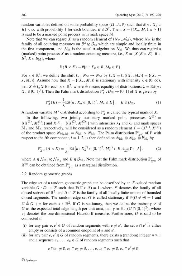
Fig. 2 Tessellation withbounded but not necessarilyconvex cells and dead ends

If, in addition to conditions (i) and (ii), it holds that

(iii) G′ = ⋃∞n=1 ∂Ξn for some random subset G′ ⊂ G of edges, where Ξ1,Ξ2, . . . :

Ω → F are bounded (but not necessarily convex) random polygons such that⋃∞n=1 Ξn = R

2, intΞi = ∅, and intΞi ∩ intΞj = ∅ for any i, j ≥ 1 with i = j

and #{n : Ξn ∩ B = ∅} < ∞ for each bounded B ∈ B2, where intΞ denotes theinner part of the set Ξ ,

then G is said to be fully connected.Let G′ ⊂ G be the maximum subset of G which satisfies the conditions mentioned

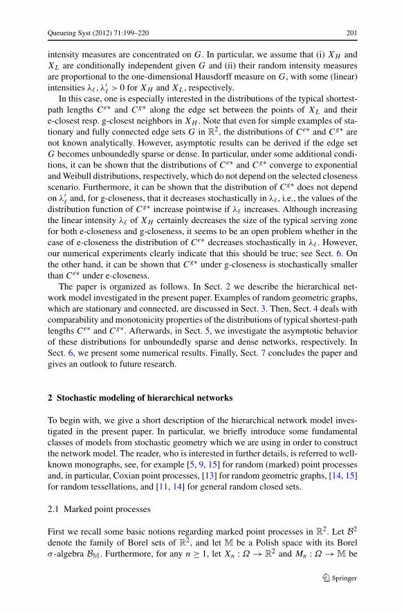
in (iii). Then, G′ can be seen as a random tessellation of the Euclidean plane withbounded but not necessarily convex cells, whereas the random set G \ intG′ can beinterpreted as a family of “dead ends”; see Fig. 2.

In the following we always assume that the random edge set G is stationary withEν1(G ∩ [0,1]2) = 1. Furthermore, for each γ > 0, we consider the scaled edge setGγ with intensity γ defined by Gγ = G/γ , i.e., we scale the edge set G such thatEν1(Gγ ∩ [0,1]2) = γ .

2.3 Serving zones and shortest path lengths

For any γ > 0, we consider stationary Cox point processes XH = {XH,n} and XL ={XL,n} whose random intensity measures are concentrated on the scaled edge setGγ = G/γ , where we assume that G satisfies the connectivity conditions (i) and(ii) introduced in Sect. 2.2. The Cox processes XH and XL are used in order tomodel the locations of HLC and LLC. In particular, we assume that (i) XH and XL

are conditionally independent given Gγ and (ii) their random intensity measures areproportional to the one-dimensional Hausdorff measure ν1 on Gγ , i.e., EXH (B) =λ�Eν1(B ∩ Gγ ) and EXL(B) = λ′

�Eν1(B ∩ Gγ ) for each Borel set B ∈ B2 and forsome (linear) intensities λ�,λ

′� > 0. Thus, the Cox processes XH and XL can be

constructed by placing homogeneous Poisson processes on the edges of Gγ withlinear intensity λ� and λ′

�, respectively. Note that the planar intensities λ and λ′ ofXH and XL are given by λ = λ�γ and λ′ = λ′

�γ .

204 Queueing Syst (2012) 71:199–220

Each LLC is assumed to be connected to its closest HLC, where two differentnotions of closeness are considered: either with respect to the Euclidean distance(e-closeness) or in a graph-theoretic sense, i.e., along the edges of the graph (g-closeness); see Fig. 1.

In the first case, we consider the Voronoi tessellation TH = {ΞH,n} induced by thepoints XH,n of the Cox process XH = {XH,n}, i.e.,

ΞH,n = {x ∈ R

2 : |x − XH,n| ≤ |x − XH,m| for all m = n},

where | · | denotes the Euclidean norm. The Voronoi cell ΞH,n is considered to bethe serving zone of the HLC located at XH,n. Furthermore let us denote by Se

H,n =(Gγ ∩ ΞH,n) − XH,n the segment system of the serving zone ΞH,n corresponding toXH,n, centered at the origin o.

We can then construct the stationary marked point process XL,Ce = {(XL,n,Cen)},

where the mark Cen is the length of the shortest path from XL,n to XH,j along the

edge set Gγ , provided that XL,n ∈ ΞH,j . Thus, each LLC is connected to that HLCwhich is closest to it in the Euclidean sense.

In the second case, the segment system centered at o of the serving zone of XH,n,denoted by S

gH,n, corresponds to the Voronoi cell S

gH,n in the graph metric, i.e.,

SgH,n = {

x ∈ Gγ : c(x,XH,n) ≤ c(x,XH,m) for all m ≥ 1} − XH,n,

where c(x,XH,n) denotes the length of the shortest path from x ∈ Gγ to XH,n alongthe edge set Gγ . Similar as above, we regard the stationary marked point processXL,Cg = {(XL,n,C

gn )}, where the mark C

gn = minm≥1(c(XL,n,XH,m)) is the mini-

mal length of shortest paths from XL,n to the points of XH along the edges of Gγ .Thus, each LLC is connected to that HLC which is closest to it in a graph-theoreticsense.

3 Examples

3.1 Stationary tessellations with convex cells

As an example of a random geometric graph, whose edge set G is fully connected,we consider the edge set of a random tessellation T = {Ξn,n ≥ 1} of R

2 with convexcells, i.e., G = G′ = ⋃∞

n=1 ∂Ξn, where Ξ1,Ξ2, . . . : Ω → F are bounded and convexrandom polygons such that

⋃∞n=1 Ξn = R

2, intΞi = ∅, and intΞi ∩ intΞj = ∅ forany i, j ≥ 1 with i = j and #{n : Ξn ∩ B = ∅} < ∞ for each bounded B ∈ B2.

Special emphasis will be put on three classes of stationary tessellations, whichare induced by homogeneous Poisson point processes: isotropic Poisson line tessel-lations (PLT), Poisson–Voronoi tessellations (PVT), and Poisson–Delaunay tessella-tions (PDT), see also [8, 17, 18]. Note that the edge set of a PVT is shown in Fig. 1.

3.2 Aggregate tessellations

Stationary tessellations with bounded, but not necessarily convex, cells can be con-structed, for example in the following way; see [2, 16]. For example, let X(1) = {X(1)

n }

Queueing Syst (2012) 71:199–220 205

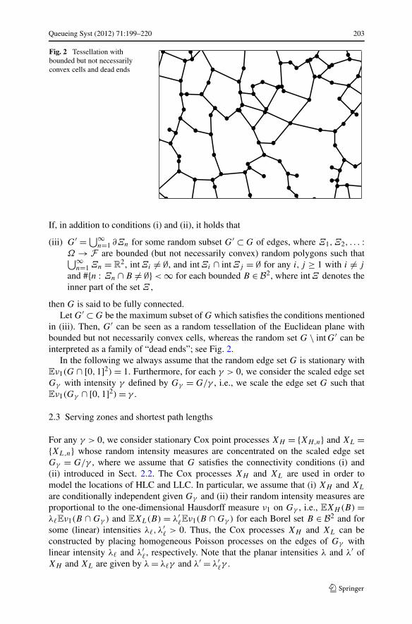
Fig. 3 Construction principle (left) and realization (right) of a PVAT with bounded nonconvex cells

and X(2) = {X(2)n } be two independent homogeneous Poisson processes. Let T (1) =

{Ξ(1)n } and T (2) = {Ξ(2)

n } denote the PVT induced by X(1) and X(2), respectively.Then, the sequence of random closed sets T = {Ξn} with

Ξn =⋃

i:X(2)i ∈Ξ

(1)n

Ξ(2)i (3)

is called an aggregate Poisson–Voronoi tessellation (PVAT) induced by X(1) and X(2).It is not difficult to see that the random edge set G = ⋃∞

n=1 ∂Ξn induced by the cellsΞn given in (3) is stationary and fully connected, see Fig. 3. Furthermore, a PVATdoes not have dead ends, i.e., G = G′.

3.3 β-skeletons

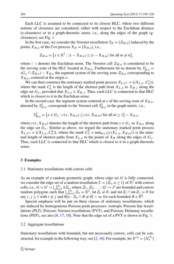
Another interesting class of geometric graphs with connected edge set is formed byβ-skeletons, first introduced in [10]. Let β ∈ [1,2], and let I ⊂ R

d be a locally finiteset. The β-skeleton G(β, I) is the edge set of a graph with vertex set I , which isdefined as follows. For x, y ∈ I , let

m(1)xy = β

2x +

(1 − β

2

)y, m(2)

xy =(

1 − β

2

)x + β

2y,

and

Aβ(x, y) = B(m(1)

xy ,∣∣m(1)

xy − y∣∣) ∩ B

(m(2)

xy ,∣∣m(2)

xy − x∣∣), (4)

where B(z, r) = {z′ ∈ R2 : |z − z′| < r} denotes the open ball with center at z ∈ R

2

and radius r ≥ 0, see Fig. 4. Then we put

G(β, I) =⋃

x,y∈I : I∩Aβ(x,y)=∅[x, y]. (5)

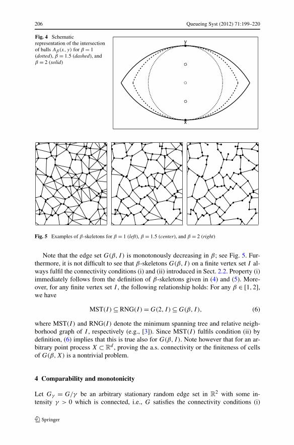
206 Queueing Syst (2012) 71:199–220

Fig. 4 Schematicrepresentation of the intersectionof balls Aβ(x, y) for β = 1(dotted), β = 1.5 (dashed), andβ = 2 (solid)

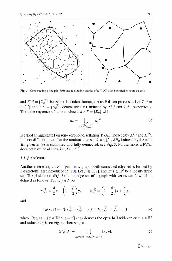
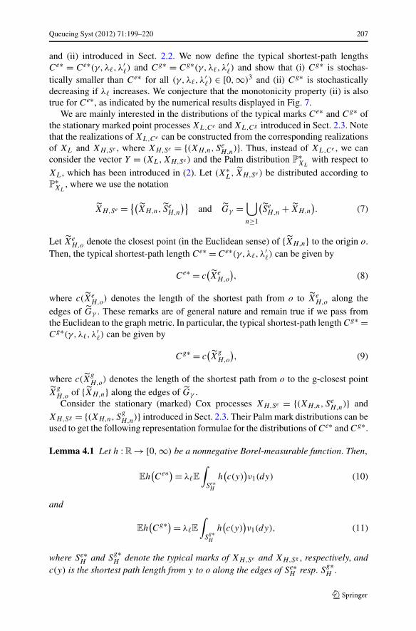
Fig. 5 Examples of β-skeletons for β = 1 (left), β = 1.5 (center), and β = 2 (right)

Note that the edge set G(β, I) is monotonously decreasing in β; see Fig. 5. Fur-thermore, it is not difficult to see that β-skeletons G(β, I) on a finite vertex set I al-ways fulfil the connectivity conditions (i) and (ii) introduced in Sect. 2.2. Property (i)immediately follows from the definition of β-skeletons given in (4) and (5). More-over, for any finite vertex set I , the following relationship holds: For any β ∈ [1,2],we have

MST(I ) ⊆ RNG(I ) = G(2, I ) ⊆ G(β, I), (6)

where MST(I ) and RNG(I ) denote the minimum spanning tree and relative neigh-borhood graph of I , respectively (e.g., [3]). Since MST(I ) fulfils condition (ii) bydefinition, (6) implies that this is true also for G(β, I). Note however that for an ar-bitrary point process X ⊂ R

d , proving the a.s. connectivity or the finiteness of cellsof G(β,X) is a nontrivial problem.

4 Comparability and monotonicity

Let Gγ = G/γ be an arbitrary stationary random edge set in R2 with some in-

tensity γ > 0 which is connected, i.e., G satisfies the connectivity conditions (i)

Queueing Syst (2012) 71:199–220 207

and (ii) introduced in Sect. 2.2. We now define the typical shortest-path lengthsCe∗ = Ce∗(γ,λ�, λ

′�) and Cg∗ = Cg∗(γ,λ�, λ

′�) and show that (i) Cg∗ is stochas-

tically smaller than Ce∗ for all (γ,λ�, λ′�) ∈ [0,∞)3 and (ii) Cg∗ is stochastically

decreasing if λ� increases. We conjecture that the monotonicity property (ii) is alsotrue for Ce∗, as indicated by the numerical results displayed in Fig. 7.

We are mainly interested in the distributions of the typical marks Ce∗ and Cg∗ ofthe stationary marked point processes XL,Ce and XL,Cg introduced in Sect. 2.3. Notethat the realizations of XL,Ce can be constructed from the corresponding realizationsof XL and XH,Se , where XH,Se = {(XH,n, S

eH,n)}. Thus, instead of XL,Ce , we can

consider the vector Y = (XL,XH,Se ) and the Palm distribution P∗XL

with respect to

XL, which has been introduced in (2). Let (X∗L, XH,Se ) be distributed according to

P∗XL

, where we use the notation

XH,Se = {(XH,n, S

eH,n

)}and Gγ =

⋃

n≥1

(Se

H,n + XH,n

). (7)

Let XeH,o denote the closest point (in the Euclidean sense) of {XH,n} to the origin o.

Then, the typical shortest-path length Ce∗ = Ce∗(γ,λ�, λ′�) can be given by

Ce∗ = c(Xe

H,o

), (8)

where c(XeH,o) denotes the length of the shortest path from o to Xe

H,o along the

edges of Gγ . These remarks are of general nature and remain true if we pass fromthe Euclidean to the graph metric. In particular, the typical shortest-path length Cg∗ =Cg∗(γ,λ�, λ

′�) can be given by

Cg∗ = c(X

gH,o

), (9)

where c(XgH,o) denotes the length of the shortest path from o to the g-closest point

XgH,o of {XH,n} along the edges of Gγ .Consider the stationary (marked) Cox processes XH,Se = {(XH,n, S

eH,n)} and

XH,Sg = {(XH,n, SgH,n)} introduced in Sect. 2.3. Their Palm mark distributions can be

used to get the following representation formulae for the distributions of Ce∗ and Cg∗.

Lemma 4.1 Let h : R → [0,∞) be a nonnegative Borel-measurable function. Then,

Eh(Ce∗) = λ�E

∫

Se∗H

h(c(y)

)ν1(dy) (10)

and

Eh(Cg∗) = λ�E

∫

Sg∗H

h(c(y)

)ν1(dy), (11)

where Se∗H and S

g∗H denote the typical marks of XH,Se and XH,Sg , respectively, and

c(y) is the shortest path length from y to o along the edges of Se∗H resp. S

g∗H .

208 Queueing Syst (2012) 71:199–220

Proof Having in mind that C∗e and S∗eH are the typical marks of the jointly stationary

marked point processes XL,C and XH,Se , formula (10) easily follows from Neveu’sexchange formula, see [12]. Formula (11) is obtained in the same way. �

From (10) and (11) it can be seen that the distributions of Ce∗ and Cg∗ do notdepend on λ′

�. Furthermore, the following result is true.

Proposition 4.2 For any (γ,λ�, λ′�) ∈ [0,∞)3, it holds that Cg∗ ≤st Ce∗, i.e.,

P(Cg∗ ≤ t

) ≥ P(Ce∗ ≤ t

)for all t > 0. (12)

Proof By the definitions of e-closeness and g-closeness, i.e., by the definitions ofthe random variables Xe

H,o and XgH,o introduced in Sect. 2.3 we get that c(X

gH,o) ≤

c(XeH,o) with P

∗XL

-probability 1. Thus, (12) immediately follows from (8) and (9). �

In order to show that Cg∗ = Cg∗(γ,λ�, λ′�) stochastically decreases in λ�, the

following auxiliary result is useful.

Lemma 4.3 The point process XH = {XH,n} introduced in (7) is a (non-stationary)Cox process on Gγ with linear intensity λ�, i.e., for each B ∈ B2, it holds thatEXH (B) = λ�Eν1(B ∩ Gγ ).

Proof The assertion immediately follows from Slivnyak’s theorem for stationary Coxprocesses; see, for example [15, p. 156]. �

Proposition 4.4 For any fixed (γ,λ′�) ∈ [0,∞)2, the typical shortest-path length

Cg∗ = Cg∗(γ,λ�, λ′�) stochastically decreases in λ�, i.e.,

Cg∗(γ,λ�,2, λ′�

) ≤st Cg∗(γ,λ�,1, λ′�

)if λ�,1 ≤ λ�,2. (13)

Proof For any λ� > 0, we consider the point process XH = XH,λ�introduced in (7),

which is a Cox process with linear intensity λ� according to Lemma 4.3. Given Gγ ,this means that XH,λ�

is a homogeneous Poisson process on Gγ with intensity λ�.Consequently, due to the well-known invariance property of Poisson processes withrespect to convolution, we get that for any 0 < λ�,1 ≤ λ�,2,

XH,λ�,2

d= XH,λ�,1 + XH,λ�,2−λ�,1 ,

where the Cox processes XH,λ�,1 and XH,λ�,2 are assumed to be conditionally in-dependent given Gγ . For the length c(X

gH,o(λ�)) of the shortest path from o to the

g-closest point Xg

H,0 = Xg

H,0(λ�) of XH,λ� along the edges of Gγ , this implies that

c(X

gH,o(λ�,2)

) ≤st c(X

gH,o(λ�,1)

)(14)

for any λ�,1, λ�,2 > 0 with λ�,1 ≤ λ�,2. Using (9), this completes the proof. �

Queueing Syst (2012) 71:199–220 209

Unfortunately, the argument which leads to (14) seems not to work for e-closeness.However, we conjecture that also Ce∗ = Ce∗(γ,λ�, λ

′�) stochastically decreases in λ�,

as indicated by the numerical results stated in Sect. 6.

5 Limit theorems

The study of limit cases of unboundedly sparse or dense edge sets is an importantmatter for modeling of realistic networks. The link between theoretical work and ap-plications are the parametric functions fitted to empirical distributions of typical pathlengths (see Sect. 6.2). Those formulas are embedded in specialized software andare expected to produce results for all possible densities of edges sets. The compu-tation of empirical densities for shortest paths can be done for a large range aroundmoderate density values but is not possible for very high or low ones. If theoreticalresults for limit cases exist, one can fill the gap in a way based on sound considera-tions. We investigate the asymptotic behavior of the distributions of Ce∗ and Cg∗ fortwo different cases, κ = γ /λ� → 0 and κ → ∞. First observe the simple scaling re-

lations Ce∗(γ,λ�)d= aCe∗(aγ, aλ�) and Cg∗(γ,λ�)

d= aCg∗(aγ, aλ�). Therefore itsuffices to understand the limit behaviour as κ → 0 under the additional assumptionof fixed λ�. Similarly, in the case κ → ∞ we may assume that γ → ∞ and λ� → 0in a way that λ�γ remains fixed. For κ → 0, we show in Theorem 5.1 that the distri-butions of Ce∗ and Cg∗ converge to an exponential distribution, where no additionalassumptions on the underlying random geometric graph G are needed. Furthermore,for κ → ∞, we show in Theorem 5.2 that the distributions of Ce∗ and Cg∗ convergeto a Weibull distribution, provided that G is isotropic and mixing satisfying G′ = G

and Eν21(∂Ξ∗) < ∞, where Ξ∗ denotes the typical cell of G.

We denote by Exp(δ) the exponential distribution with expectation δ−1. Further-more, Wei(a, b) denotes the Weibull distribution with scale parameter a > 0 andshape parameter b > 0.

5.1 Asymptotic exponential distribution for κ → 0

First we regard the case that κ = γ /λ� → 0 with λ� fixed, i.e., γ → 0.

Theorem 5.1 Let G be an arbitrary random geometric graph which is stationaryand connected. Then, for any fixed λ� > 0,

Ce∗(γ,λ�)d→ Z and Cg∗(γ,λ�)

d→ Z (15)

as γ → 0, whered→ denotes convergence in distribution, and Z ∼ Exp(2λ�).

Proof We can use similar arguments as in [17], where the asymptotic behavior ofCe∗ has been considered for the special case that G is the edge set of a stationary

210 Queueing Syst (2012) 71:199–220

tessellation with convex cells. Namely, it holds that limγ→0 Rγ = ∞ with P∗XL

—

probability 1, where Rγ = max{r > 0 : B(o, r)∩ Soγ = B(o, r)∩Gγ }, and So

γ denotesthe segment of Gγ containing the origin. This implies that

limγ→0

P(C∗g ≤ x | Xg

H,o ∈ B(o,Rγ )) = lim

γ→0P(C∗e ≤ x | Xe

H,o ∈ B(o,Rγ )).

Thus, in the same way as done in [17] for Ce∗ and G being the edge set of a sta-tionary tessellation with convex cells, it can be shown that Ce∗ and Cg∗ converge indistribution to the random distance from o to the nearest point of a stationary Poissonprocess on R with intensity λ�, which is Exp(2λ�)-distributed. �

5.2 Asymptotic Weibull distribution as κ → ∞

In this section we additionally assume that the stationary edge set G is isotropic andmixing. Furthermore, we assume that G is fully connected, does not possess deadends, i.e., G′ = G, and

Eν21

(∂Ξ∗) < ∞, (16)

where ν1(∂Ξ∗) denotes the circumference of the typical cell Ξ∗ of G. Then, it is notdifficult to see that the proof of Theorem 3.2 in [17] regarding the asymptotic behaviorof Ce∗(γ,λ�) as κ → ∞ remains true in the present case of a random tessellationG with not necessarily convex cells. Our goal is to show that the result derived inTheorem 3.2 of [17] also holds if we pass from Ce∗(γ,λ�) to Cg∗(γ,λ�).

Theorem 5.2 If γ → ∞ and λ� → 0 with λ�γ = λ fixed, then there exists a constantξ ≥ 1 such that

Ce∗(γ,λ�)d→ ξZ and Cg∗(γ,λ�)

d→ ξZ, (17)

where ξZ ∼ Wei(λπ/ξ2,2).

In order to show Theorem 5.2, let us recall the idea behind the proof of Theo-rem 3.2 in [17]. By an argument based on Kingman’s subadditive ergodic theorem

one can show that there exists ξ ≥ 1 such that Ce∗ − ξ |XeH,o|

P→ 0, whereP→ denotes

convergence in probability. Since |XeH,o|

d→ Wei(λπ,2), an application of Slutsky’s

lemma (see [6, Chap. 2, Exc. 2.10]) yields Ce∗ d→ Wei(λπ/ξ2,2). Moreover, thisstrategy proves to be flexible enough to handle the current situation with respect toCg∗ as well.

To show that Cg∗ d→ Wei(λπ/ξ2,2), we begin by proving an analogue ofLemma 4.4 in [17].

Lemma 5.3 Let γ → ∞ and λ� → 0 such that λ�γ = λ is fixed. Then there is a

constant ξ ≥ 1 such that Cg∗(γ,λ�) − ξ |XgH,o|

P→ 0.

Queueing Syst (2012) 71:199–220 211

Proof Let ε, δ > 0 be arbitrary. We want to prove that there exists a ξ ≥ 1 (which infact coincides with the ξ in Lemma 4.4 of [17]) such that for all γ sufficiently large,we have P(|Cg∗ − ξ |Xg

H,o|| > ε) ≤ δ. Using

P(∣∣Cg∗ − ξ

∣∣XgH,o

∣∣∣∣ > ε) = P

(∣∣Cg∗ − ξ∣∣Xg

H,o

∣∣∣∣ > ε,∣∣Xg

H,o

∣∣ ≤ r)

+ P(∣∣Cg∗ − ξ

∣∣XgH,o

∣∣∣∣ > ε,∣∣Xg

H,o

∣∣ > r),

it suffices to show that there exists r > 0 such that for all sufficiently large γ , we have

P(∣∣Cg∗ − ξ

∣∣XgH,o

∣∣∣∣ > ε,∣∣Xg

H,o

∣∣ ≤ r)< δ/2 and P

(∣∣XgH,o

∣∣ > r)< δ/2.

Using the elementary inequalities |XgH,o| ≤ c(X

gH,o) ≤ c(Xe

H,o) and Lemma 4.2 of

[17], i.e., |XeH,o|

d−→ Wei(λπ,2), we can choose r > 0 such that

P(∣∣Xg

H,o

∣∣ > r) ≤ P

(c(Xe

H,o

)> r

)

≤ P(ξ∣∣Xe

H,o

∣∣ > r/2) + P

(∣∣ξ∣∣Xe

H,o

∣∣ − c(Xe

H,o

)∣∣ > r/2)

≤ δ

4+ δ

4

for all γ > 0 sufficiently large. To prove the remaining estimate, we denote by N =XH (B(o, r)) the number of points of XH in the ball B(o, r). Using this notation, wemay write

P(∣∣Cg∗ − ξ

∣∣Xg

H,o

∣∣∣∣ > ε,

∣∣Xg

H,o

∣∣ ≤ r

)

≤ E

( ∞∑

k=1

P(N = k | Gγ

) · E

(max

i=1,...,k

∣∣c(Yi) − ξ |Yi |∣∣ > ε | Gγ , N = k

))

,

where the random vectors Y1, . . . , Yk are conditionally independent and uniformlydistributed on Gγ ∩ B(o, r) given Gγ and N . Then, in the next steps, copying thecorresponding part of the proof of Lemma 4.4 in [17] verbatim yields the assertion. �

As a second ingredient in the proof of Cg∗ d→ Wei(λπ/ξ2,2), we still need anotherauxiliary result.

Lemma 5.4 Let γ → ∞ and λ� → 0 such that λ�γ = λ is fixed. Then,

∣∣XgH,o

∣∣ − ∣∣XeH,o

∣∣ P→ 0 (18)

and, consequently,

∣∣XgH,o

∣∣ d→ Wei(λπ,2). (19)

212 Queueing Syst (2012) 71:199–220

Proof Observe that |XgH,o| − ∣∣Xe

H,o

∣∣ ≥ 0 by definition. Furthermore, for any ξ > 0.we have

P(ξ∣∣Xg

H,o

∣∣ − ξ∣∣Xe

H,o

∣∣ > ε)

= P((

ξ∣∣Xg

H,o

∣∣ − c(X

gH,o

)) + (c(X

gH,o

) − c(Xe

H,o

)) + (c(Xe

H,o

) − ξ∣∣Xe

H,o

∣∣) > ε)

≤ P(∣∣ξ

∣∣XgH,o

∣∣ − c(X

gH,o

)∣∣ > ε/2) + P

(∣∣c(Xe

H,o

) − ξ∣∣Xe

H,o

∣∣∣∣ > ε/2),

where in the last inequality we used that c(XgH,o)− c(Xe

H,o) ≤ 0. But, by Lemma 4.4of [17] and by Lemma 5.3, we know that both summands of the latter bound convergeto 0 as γ → ∞. This proves (18), and, applying Slutsky’s lemma, (19) follows by

taking into account that |XeH,o|

d→ Wei(λπ,2). �

Note that the convergence Cg∗(γ,λ�)d→ ξZ stated in Theorem 5.2 is now an

immediate consequence of Lemmas 5.3 and 5.4, because

c(X

gH,o

) = ξ∣∣Xg

H,o

∣∣ + (c(X

gH,o

) − ξ∣∣Xg

H,o

∣∣) d→ ξZ ∼ Wei(λπ/ξ2,2

).

5.3 Checking the conditions of Theorem 5.2

We now discuss some examples of G for which the conditions of Theorem 5.2 aresatisfied. If G is the edge set of a PLT, PVT, and PDT, respectively, then G is isotropicby definition, and it is well known that G is mixing, see Chap. 10.5 in [14]. Further-more, it is not difficult to show in all these cases that the integrability condition (16)is fulfilled, see [17].

Moreover, it turns out that the conditions of Theorem 5.2 are fulfilled if G is theedge set of a PVAT introduced in Sect. 3.2. Then, by definition, G is stationary andisotropic. In order to show that G is mixing, we can apply an extended version ofthe arguments which have been used in Theorem 10.5.1 of [14] for (nonaggregated)PVT.

Lemma 5.5 Let T (1) = {Ξ(1)n } and T (2) = {Ξ(2)

n } be independent Poisson–Voronoitessellations. Then the edge set G = ⋃

n≥1 ∂Ξn of the PVAT T = {Ξn} introduced in(3) is mixing.

Proof To begin with, we recall the basic ideas of the proof of Theorem 10.5.1 in [14],which have been developed there to show that any (nonaggregate) PVT T = {Ξn} ismixing, where Ξn = {x ∈ R

2 : |Xn − x| ≤ |Xi − x| for any i = n}, and X = {Xn} is ahomogeneous Poisson process. That is, for any fixed ε > 0 and bounded B1,B2 ∈ B2,

∣∣P(G ∩ B1 = ∅,G ∩ (B2 + x) = ∅)

− P(G ∩ B1 = ∅)P(G ∩ (B2 + x) = ∅)∣∣ < 6ε (20)

for all x ∈ R2 such that |x| is sufficiently large, where G = ⋃

n≥1 ∂Ξn denotes theedge set of T . In order to prove (20), the following truncation technique has been used

Queueing Syst (2012) 71:199–220 213

in [14]. For r > 0 and x ∈ R2, let Gx denote the edge set of the Voronoi tessellation

induced by the point process X ∩ B(x,15r). If |x| > 30r , then the random sets Go

and Gx are independent. This implies that

P(Go ∩ B1 = ∅,Gx ∩ (B2 + x) = ∅) = P(Go ∩ B1 = ∅)P

(Gx ∩ (B2 + x) = ∅)

.

The next step in the proof of Theorem 10.5.1 given in [14], which yields (20), is toshow that one can choose r > 0 such that∣∣P

(Go ∩ B1 = ∅,Gx ∩ (B2 + x) = ∅) − P

(G ∩ B1 = ∅,G ∩ (B2 + x) = ∅)∣∣ < 2ε,

∣∣P(Go ∩ B1 = ∅) − P(G ∩ B1 = ∅)∣∣ < 2ε, (21)

∣∣P

(Gx ∩ (B2 + x) = ∅) − P

(G ∩ (B2 + x) = ∅)∣∣ < 2ε

for all x ∈ R2 with |x| sufficiently large. To achieve this goal, one first introduces the

following family of events (parameterized by y ∈ R2 and r > 0):

Eyr = {

ω ∈ Ω : Ξn(ω) ∩ B(y, r) = ∅,Ξn(ω) ⊂ B(y,5r) for some n ≥ 1}.

It is not difficult to see that for r > 0 sufficiently large, we have P(Eyr ) = P(Eo

r ) < ε

for all y ∈ R2. This yields P(F x1,x2) ≥ 1 − 2ε for any x1, x2 ∈ R

2, where Fx1,x2r =

(Ex1r ∪E

x2r )c . The benefit of introducing the events E

yr and F

x1,x2r is as follows. First

choose r > 0 large enough such that B1,B2 ⊂ B(o, r). Now suppose that ω ∈ Fx1,x2r

and Ξn(ω) ∩ (Bi + xi) = ∅ for some n ≥ 1 and i ∈ {1,2}. Then Ξn(ω) ⊂ B(xi,5r).Using elementary geometry, it is easy to see that this implies that the Voronoi cellΞn(ω) is completely determined by X ∩ B(xi,15r). Thus, G ∩ (Bi + xi) = ∅ if andonly if Gxi

∩ (Bi + xi) = ∅ implying the inequalities in (21). The basic ideas of thisapproach may also be used in the case of PVAT. Denote by X(1) and X(2) independentPoisson processes inducing the PVT T (1) = {Ξ(1)

n } and T (2) = {Ξ(2)n }, respectively.

For y ∈ R2 and r > 0, let

Eyr = {

ω ∈ Ω : Ξ(2)n (ω) ∩ B(y, r) = ∅,Ξ(2)

n (ω) ⊂ B(y,5r) for some n ≥ 1}

∪ {ω ∈ Ω : Ξ(1)

n (ω) ∩ B(y,5r) = ∅,Ξ(1)n (ω) ⊂ B(y,25r) for some n ≥ 1

}

∪ {ω ∈ Ω : Ξ(2)

n (ω) ∩ B(y,25r) = ∅,Ξ(2)n (ω) ⊂ B(y,125r) for some n ≥ 1

}.

Then, as in the case of a (nonaggregate) PVT mentioned above, it is easy to seethat for r > 0 sufficiently large, we have P(E

yr ) = P(Eo

r ) < ε for all y ∈ R2 and

P(F x1,x2) ≥ 1 − 2ε for any x1, x2 ∈ R2, where F

x1,x2r = (E

x1r ∪ E

x2r )c . Furthermore,

if ω ∈ Fx1,x2r , then Ξn(ω) ∩ (Bi + xi) = ∅ for some n ≥ 1 and i ∈ {1,2} implies

that Ξn(ω) ⊂ B(xi,125r), where T = {Ξn} is the PVAT induced by X(1) and X(2).Thus, in this case, the cell Ξn is completely determined by X(1) ∩ B(xi,375r) andX(2) ∩ B(xi,375r), and the proof can be finished in the same way as indicated abovefor (nonaggregate) PVT. �

Finally, we show that the integrability condition (16) is fulfilled if G is the edgeset of a PVAT.

214 Queueing Syst (2012) 71:199–220

Lemma 5.6 Let T (1) = {Ξ(1)n } and T (2) = {Ξ(2)

n } be Voronoi tessellations induced bythe stationary and independent point processes X(1) = {X(1)

n } and X(2) = {X(2)n } with

intensities λ(1) and λ(2). Assume that E(ν42(Ξ(1),∗)) < ∞ and E(ν4

1(∂Ξ(2),∗)) < ∞,where Ξ(1),∗ and Ξ(2),∗ denotes the typical cell of T (1) and T (2), respectively. IfX(2) = {X(2)

n } is a homogeneous Poisson process, then E(ν21(∂Ξ∗)) < ∞, where Ξ∗

is the typical cell of the aggregate tessellation T = {Ξn} induced by X(1) and X(2).

Proof Consider the marked point processes Y (1) = {(X(1)n ,Ξ

(1)n − X

(1)n )} and Y (2) =

{(X(2)n ,Ξ

(2)n − X

(2)n )}. Let P

o1 denote the Palm mark distribution of Y (1), see (1), and

let C2 be the Campbell measure of Y (2), i.e.,

C2(B × E × A) = E(#{n : X(2)

n ∈ B,Ξ(2)n − X(2)

n ∈ E}1A

(X(2)

)),

where B ∈ B2, E ∈ B F , and A ∈ N . Then, using (1) and (3), we get

E(ν2

1

(∂Ξ∗)) ≤ 1

λ(1)E

( ∑

n:X(1)n ∈[0,1]2

( ∑

i:X(2)i ∈Ξ

(1)n

ν1(∂Ξ

(2)i

))2)

≤ 1

λ(1)E

( ∑

n:X(1)n ∈[0,1]2

X(2)(Ξ(1)

n

) ∑

i:X(2)i ∈Ξ

(1)n

ν21

(∂Ξ

(2)i

)).

Thus, using Campbell’s theorem for stationary marked point processes (see, for ex-ample [5, 15]), this gives

E(ν2

1

(∂Ξ∗)) ≤

∫

[0,1]2

∫

F

∫

R2×F ×N

1m1+x(y)ϕ(m1 + x)ν21(∂m2)

× C2(dy, dm2, dϕ)Po1(dm1) dx

≤∫

[0,1]2

∫

F

(∫

R2×F ×N

1m1+x(y)ϕ2(m1 + x)C2(dy, dm2, dϕ)

)1/2

×(∫

R2×F ×N

1m1+x(y)ν41(∂m2)C2(dy, dm2, dϕ)

)1/2

Po1(dm1) dx.

Furthermore, by the definition of the typical cell Ξ(2),∗, we have∫

R2×F ×N

1m1+x(y)ν41 (∂m2)C2(dy, dm2, dϕ) = λ(2)ν2(m1)Eν4

1

(∂Ξ(2),∗),

and applying Slivnyak’s theorem (see [5, 15]) to the homogeneous Poisson processX(2) gives that

∫

R2×F ×N

1m1+x(y)ϕ2(m1 + x)C2(dy, dm2, dϕ)

= (λ(2)

)2ν3

2(m1) + 3λ(2)ν22(m1) + ν2(m1).

Queueing Syst (2012) 71:199–220 215

Thus, we get that

E(ν2

1

(∂Ξ∗)) ≤ (

λ(2)Eν4

1

(∂Ξ(2),∗))1/2

∫

F

((λ(2)

)2ν4

2(m1) + 3λ(2)ν23(m1)

+ ν22(m1)

)1/2P

o1(dm1)

≤ (λ(2)

Eν41

(∂Ξ(2),∗))1/2(

E(ν2

2

(Ξ(1),∗)) + 3λ(2)

E(ν3

2

(Ξ(1),∗))

+ (λ(2)

)2E

(ν4

2

(Ξ(1),∗)))1/2

,

where the latter bound is finite, because we assumed that E(ν42(Ξ(1),∗)) < ∞ and

E(ν41(∂Ξ(2),∗)) < ∞. �

Corollary 5.7 If both X(1) and X(2) are homogeneous Poisson processes, thenE(ν2

1(∂Ξ∗)) < ∞, where Ξ∗ is the typical cell of the PVAT T = {Ξn} induced byX(1) and X(2).

Proof Let B ∈ B2 be bounded and convex, and denote by R(B) the radius of thesmallest ball containing B . By the convexity of B it holds that ν1(∂B) ≤ 2πR(B)

and ν2(B) ≤ πR2(B). Thus, by the result of Lemma 5.6, it is sufficient to show thatall moments of R(Ξ(i),∗) are finite, where Ξ(i),∗ denotes the typical cell of the PVTT (i) for i ∈ {1,2}. But this follows from a result derived in [7] (see also [4]), whereit is shown that R(Ξ(i),∗) has exponential tails. �

6 Numerical results

6.1 Simulation-based density estimators

The aim of this section is to consider simulation-based estimators for the densities ofthe typical shortest-path lengths Ce∗ and Cg∗. In particular, we construct an estimatorfor the density fCg∗(x) of Cg∗ based on n independent and identically distributedsamples of the typical segment system S

g∗H , similar to the estimator fCe∗(x;n) for the

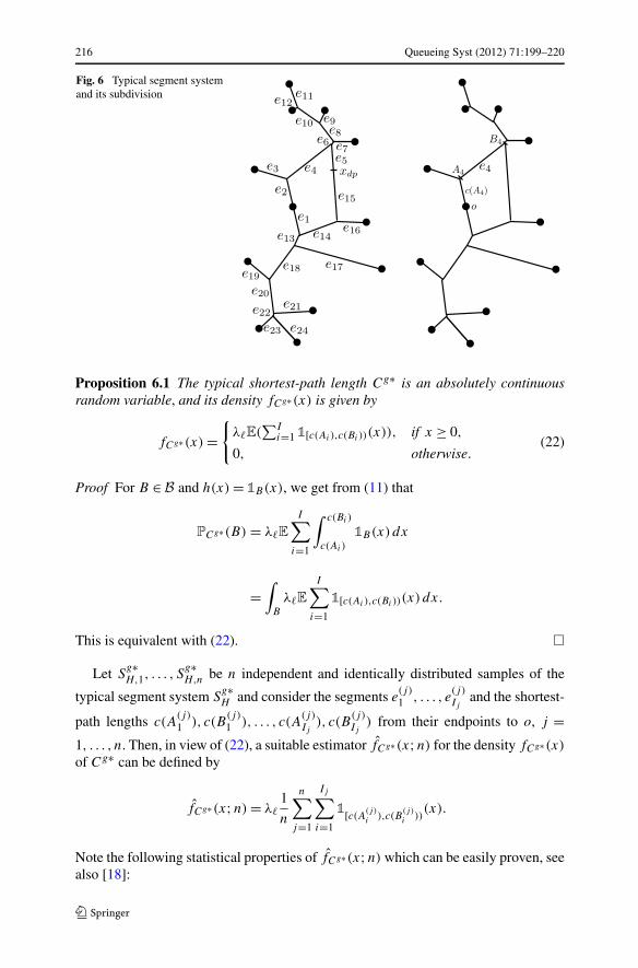
density of Ce∗ introduced in [18].To achieve this goal, it is useful to decompose the typical segment system S

g∗H ,

i.e., we subdivide Sg∗H into N parts, its segments e1, . . . , eI , and denote by Ai and Bi ,

i ∈ {1, . . . , I }, the endpoints of these segments (see Fig. 6) such that:

– S∗,gH = ⋃I

i=1 ei ,– ν1(ei ∩ ej ) = 0 for i = j , and– c(Ai) < c(Bi) = c(Ai) + ν1(ei).

Note that it can sometimes happen that so-called distance peaks occur. A point xdp iscalled distance peak if there exist two different shortest paths from o to xdp . There-fore, some segments are subdivided into two parts at xdp (see Fig. 6).

In the same way as done in Theorem 1 of [18] for the density of Ce∗, the followingresult is obtained.

216 Queueing Syst (2012) 71:199–220

Fig. 6 Typical segment systemand its subdivision

Proposition 6.1 The typical shortest-path length Cg∗ is an absolutely continuousrandom variable, and its density fCg∗(x) is given by

fCg∗(x) ={

λ�E(∑I

i=1 1[c(Ai),c(Bi))(x)), if x ≥ 0,

0, otherwise.(22)

Proof For B ∈ B and h(x) = 1B(x), we get from (11) that

PCg∗(B) = λ�E

I∑

i=1

∫ c(Bi)

c(Ai)

1B(x)dx

=∫

B

λ�E

I∑

i=1

1[c(Ai),c(Bi))(x) dx.

This is equivalent with (22). �

Let Sg∗H,1, . . . , S

g∗H,n be n independent and identically distributed samples of the

typical segment system Sg∗H and consider the segments e

(j)

1 , . . . , e(j)Ij

and the shortest-

path lengths c(A(j)

1 ), c(B(j)

1 ), . . . , c(A(j)Ij

), c(B(j)Ij

) from their endpoints to o, j =1, . . . , n. Then, in view of (22), a suitable estimator fCg∗(x;n) for the density fCg∗(x)

of Cg∗ can be defined by

fCg∗(x;n) = λ�

1

n

n∑

j=1

Ij∑

i=1

1[c(A(j)i ),c(B

(j)i ))

(x).

Note the following statistical properties of fCg∗(x;n) which can be easily proven, seealso [18]:

Queueing Syst (2012) 71:199–220 217

Fig. 7 Densities (left) and distribution functions (right) of Ce∗ for PVT, where κ = 10 (solid), κ = 20(dashed), κ = 50 (dotted), κ = 100 (dotdashed)

(1) EfCg∗(x;n) = fCg∗(x) for each x ∈ R,(2) P(limn→∞ supx∈R |fCg∗(x;n) − fCg∗(x)|) = 1,(3) Eh(Cg∗) = E[∫

Rh(x)fCg∗(x;n)dx] for each measurable h : R �→ [0,∞).

6.2 Empirical distributions of Ce∗ and Cg∗

As mentioned in Sect. 4, it is natural to conjecture that the typical shortest-pathlengths Ce∗ = Ce∗(γ,λ�, λ

′�) are stochastically decreasing in λ�. In Fig. 7 we have

plotted densities and distribution functions of the estimated typical shortest-pathlength Ce∗ for the case of e-closeness, where G is the edge set of a PVT, and theestimator fCe∗(x;n) for the density of Ce∗ introduced in [18] has been used. Thefour plots correspond to κ = 10,20,50,100, respectively (where we fixed γ = 1 andn = 2000 iterations). It is clearly visible that the distribution functions on the right-hand side of Fig. 7 do not intersect and that each pair of density functions on theleft-hand side of Fig. 7 intersect only once. These two observations provide strongindications for the stochastic monotonicity of the respective typical shortest-pathlengths Ce∗. Similar results have been obtained for other classes of stationary tessel-lations with convex cells, see also [17, 18] for PLT and PDT. However, we were notable to provide a proof of this monotonicity property. However, recall that in contrastto this situation for e-closeness, the stochastic monotonicity of Cg∗ = Cg∗(γ,λ�, λ

′�)

can formally be shown, see Proposition 4.4.Furthermore, recall that in Proposition 4.2 we showed that Ce∗ is always stochas-

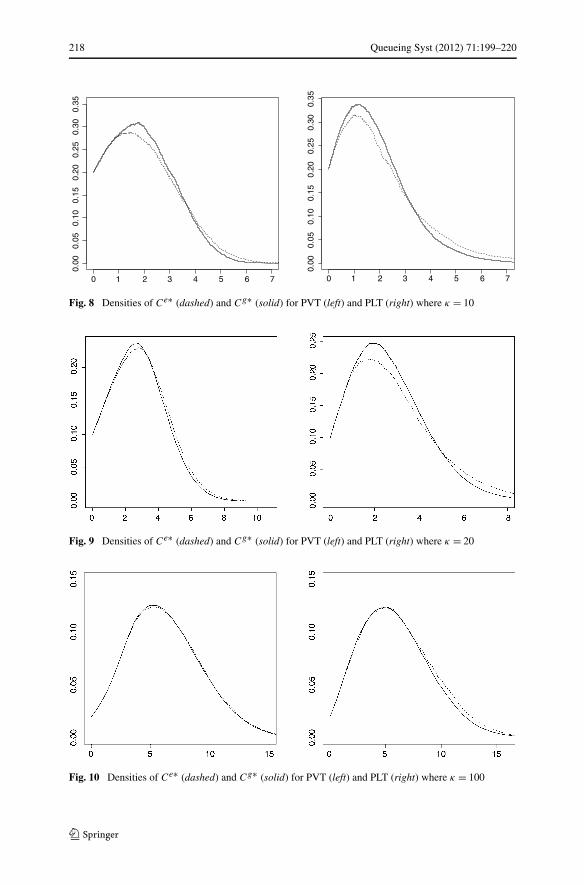
tically larger than Cg∗. We evaluated the simulation-based density estimatorsfCg∗(x;n) and fCe∗(x;n) mentioned in Sect. 6.1 for n = 2000 simulations, in orderto find out how much larger Ce∗ is than Cg∗ for given specifications of the parametervector (γ,λ�, λ

′�). From Figs. 8 and 9 we see that the empirical densities fCg∗(x;n)

and fCe∗(x;n) are quite different from each other for κ = 10 and κ = 20, whereasfor κ = 100, this is not the case (at least not for PVT), see Fig. 10. Note that the latterphenomenon is in accordance with the result of Theorem 5.2, which states that thedistributions of Ce∗ and Cg∗ converge to the same limit as κ → ∞.

218 Queueing Syst (2012) 71:199–220

Fig. 8 Densities of Ce∗ (dashed) and Cg∗ (solid) for PVT (left) and PLT (right) where κ = 10

Fig. 9 Densities of Ce∗ (dashed) and Cg∗ (solid) for PVT (left) and PLT (right) where κ = 20

Fig. 10 Densities of Ce∗ (dashed) and Cg∗ (solid) for PVT (left) and PLT (right) where κ = 100

Queueing Syst (2012) 71:199–220 219

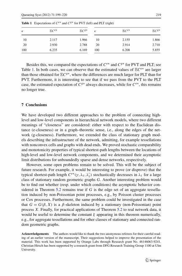
Table 1 Expectations of Ce∗ and Cg∗ for PVT (left) and PLT (right)

κ ECe∗ECg∗

10 2.117 1.966

20 2.930 2.788

100 6.235 6.169

κ ECe∗ECg∗

10 2.155 1.866

20 2.914 2.710

100 6.208 5.855

Besides this, we compared the expectations of Ce∗ and Cg∗ for PVT and PLT; seeTable 1. In both cases, we can observe that the estimated values of ECe∗ are largerthan those obtained for ECg∗, where the differences are much larger for PLT than forPVT. Furthermore, it is interesting to see that if we pass from the PVT to the PLTcase, the estimated expectation of Cg∗ always decreases, while for Ce∗, this remainsno longer true.

7 Conclusions

We have developed two different approaches to the problem of connecting high-level and low-level components in hierarchical network models, where two differentmeanings of “closeness” are considered: either with respect to the Euclidean dis-tance (e-closeness) or in a graph–theoretic sense, i.e., along the edges of the net-work (g-closeness). Furthermore, we extended the class of stationary graph mod-els describing the infrastructure of the network, admitting, for example tessellationswith nonconvex cells and graphs with dead ends. We proved stochastic comparabilityand monotonicity properties of typical shortest-path lengths between the locations ofhigh-level and low-level network components, and we determined their asymptoticlimit distributions for unboundedly sparse and dense networks, respectively.

However, some open problems remain to be solved. This will be the subject offuture research. For example, it would be interesting to prove (or disprove) that thetypical shortest-path length Ce∗(γ,λ�, λ

′�) stochastically decreases in λ� for a large

class of stationary random geometric graphs G. Another interesting problem wouldbe to find out whether (resp. under which conditions) the asymptotic behavior con-sidered in Theorem 5.2 remains true if G is the edge set of an aggregate tessella-tion induced by non-Poissonian point processes, e.g., by Poisson cluster processesor Cox processes. Furthermore, the same problem could be investigated in the casethat G = G(β,X) is a β-skeleton induced by a stationary (non-Poissonian) pointprocess X. Finally, for practical applications of Theorem 5.2 to real network data, itwould be useful to determine the constant ξ appearing in this theorem numerically,e.g., for aggregate tessellations and for other classes of stationary and connected ran-dom geometric graphs.

Acknowledgements The authors would like to thank the two anonymous referees for their careful read-ing of an earlier version of the manuscript. Their suggestions helped to improve the presentation of thematerial. This work has been supported by Orange Labs through Research grant No. 46146063-9241.Christian Hirsch has been supported by a research grant from DFG Research Training Group 1100 at UlmUniversity.

220 Queueing Syst (2012) 71:199–220

References

1. Aldous, D., Shun, J.: Connected spatial networks over random points and a route-length statistic. Stat.Sci. 25, 275–288 (2010)

2. Baccelli, F., Gloaguen, G., Zuyev, S.: Superposition of planar Voronoi tessellations. Stoch. Models16, 69–98 (2000)

3. Bose, P., Devroye, L., Evans, W., Kirkpatrick, D.: On the spanning ratio of Gabriel graphs andβ-skeletons. In: Proceedings of the 5th Latin American Symposium on Theoretical Informatics(LATIN’02). Lecture Notes in Computer Science, vol. 2286, pp. 479–493. Springer, Berlin (2002)

4. Calka, P.: The distributions of the smallest disks containing the Poisson–Voronoi typical cell and theCrofton cell in the plane. Adv. Appl. Probab. 34, 702–717 (2002)

5. Daley, D.J., Vere-Jones, D.: An Introduction to the Theory of Point Processes, vols. I/II. Springer,New York (2005/2008)

6. Durrett, R.: Probability: Theory and Examples, 2nd edn. Duxbury, Belmont (1996)7. Foss, S.G., Zuyev, S.A.: On a Voronoi aggregative process related to a bivariate Poisson process. Adv.

Appl. Probab. 28, 965–981 (1996)8. Gloaguen, C., Voss, F., Schmidt, V.: Parametric distributions of connection lengths for the efficient

analysis of fixed access network. Ann. Télécommun. 66, 103–118 (2011)9. Illian, J., Penttinen, A., Stoyan, H., Stoyan, D.: Statistical Analysis and Modelling of Spatial Point

Patterns. Wiley, New York (2008)10. Kirkpatrick, D.G., Radke, J.D.: A framework for computational morphology. In: Toussaint, G.T. (ed.)

Computational Geometry, pp. 217–248. North Holland, Amsterdam (1985)11. Molchanov, I.S.: Theory of Random Sets. Springer, London (2005)12. Neveu, J.: Processus ponctuels. In: École d’Été de Probabilités de Saint-Flour VI. Lecture Notes in

Mathematics, vol. 598, pp. 249–445. Springer, Berlin (1977)13. Penrose, M.: Random Geometric Graphs. Oxford University Press, Oxford (2003)14. Schneider, R., Weil, W.: Stochastic and Integral Geometry. Springer, Berlin (2008)15. Stoyan, D., Kendall, W.S., Mecke, J.: Stochastic Geometry and Its Applications. Wiley, New York

(1995)16. Tchoumatchenko, K., Zuyev, S.: Aggregate and fractal tessellations. Probab. Theory Relat. Fields

121, 198–218 (2001)17. Voss, F., Gloaguen, C., Schmidt, V.: Scaling limits for shortest path lengths along the edges of station-

ary tessellations. Adv. Appl. Probab. 42, 936–952 (2010)18. Voss, F., Gloaguen, C., Fleischer, F., Schmidt, V.: Densities of shortest path lengths in spatial stochas-

tic networks. Stoch. Models 27, 141–167 (2011)