Embed Size (px)
Citation preview
Vol. 16 No. 1 CHIN. J. OCEANOL. LIMNOL. 1998
ON THE EXCHANGE FLOW IN TIDAL RIVERS AND SHALLOW ESTUARIES*
LI Chun-yan ( ~ ~ ) (CCPO, Old Dominion University, Viroinia )
James O' Donnell ( Department o f Marine Sciences, University of Conneaicut, Groton, CT )
Received March 26, 1997; revision accepted July 26, 1997
Abstract An analytic model is developed to investigate the barotropic tidally driven residual ex-
change flow in shallow estuaries. Ebb dominated flow in deep channel and flood dominated flow on the
shoals produced by the model are consistent with some observatiom in tidal rivels and shallow estuaries.
Analysis shows that this type of exchange flow is caused by the combined effect of nonlinearity and the
lateral ~ariation of the depth. The inward flux is mainly due to the surface elevation of the wave. A
seav, ard residual pressure gradient has to be maintained to drive the water outward for mass balance. Since
the surface elevation in an estuary has only small lateral variation, the depth integrated pressure force is
mainly dependent on the depth whose value in the channel is larger than that on the shoals. As a result, the
return flow in the channel is larger than that on the shoals. An ebb-flood flow system is thus generated.
Key wor~ tide, residual circulation, sub-tidal, exchange flow, shallow estuary, analytic solution
INTRODUCTION
The well known theories of Pritchard (1952) and Hansen and Rattray (1965) describe estuarine circulation as freshened seawater flowing out in a near surface layer and seawater flowing landward below. When the lateral variation of bathyr~try is taken into account, the vertical stratification may be replaced, or partially replaced, by a lateral stratification along with a lateral variation of velocity field, which may show a landward flow of salt water in the deep channel and seaward flow of fresher water on the shoals, This mode of baroclinic circulation was first suggested by Fischer (1972), and further explained and ob- served by Hamrick (1979)and Wong (1994).
However, observations do not always reveal this mode of circulation. Robinson (1960, 1965) indicated that narrow estuaries often have a dominant ebb channel. Observations by Zim- merman (1974), Charlton et al. (1975), Kjerfve (1978, 1986) also showed that the ebb directed flow tended to concentrate in the main channel, with flood directed flow on the shoals. In addition, the results of Kjerfve(1986) showed that the maximum residual flow varied with the amplitude of the semi~liumal tide between the spring and the neap. This indicates that the exchange flow may be tidally induced.
In this paper, a theory is presented for the tidally driven(barotropic) residual ex- change flow in a channel with lateral depth variations. Explanations for the observed ebb-flood flow system is provided.
THE THEORY
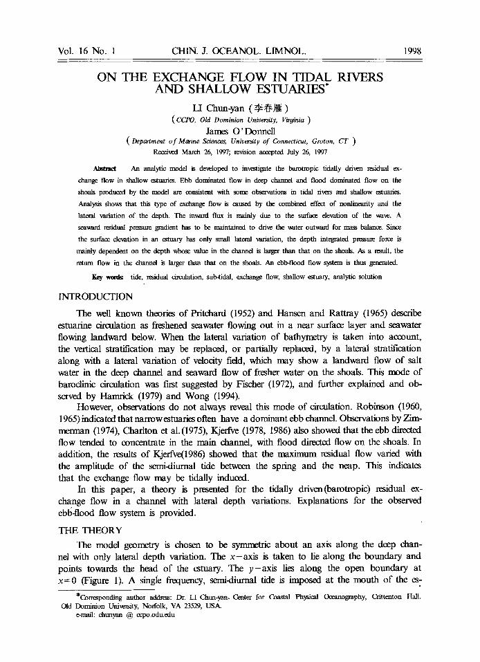
The model geometry is chosen to be symmetric about an axis along the deep chan- nel with only lateral depth variation. The x-axis is taken to lie along the boundary and points towards the head of the estuary. The y-ax is lies along the open boundary at x = 0 (Figure 1). A single frequency, semi~liumal tide is imposed at the mouth of the es-
*Corresponding author address: Dr. LI Chun-yan, Center for Coastal Physical Oceanography, Crittenton HalL Old Dominion University, Norfolk, VA 23529, USA.
e-mail: chunyan @ ccpo.odu.edu
2 CHINESE JOURNAL OF OCEANOLOGY AND LIMNOLOGY Vol.16
tuary. Both the amplitude and phase of sea level variation are assumed to be uniform across the estuary and are specified. Since the Coriolis effect is neglected, the flow is symrmtric about the central axis of the estuary (y=D) . It is, therefore, only necessary to discuss the problem within half of the estuary (0 < y < D).
The depth-averaged shallow water momentum and continuity equations are used(L i, 1996)
Ou Ou Ou = O F u fl u( (1) at +u-~x +v ay - g ~ x - # ~ +--~- av av av _ a~ v # v~ + u ~ + v (2) ~ -g-~y -#~- +
(3) d~ tg(h+Ou ~ ~(h+~)v ~--f + dx dy =0
8Co a h~ )1/3, where u, v, ~, h, x, y, t, Co, h0, L0, a and g in which t = 3rr ho x/~o (CoaLo are along channel velocity, lateral velocity, elevation, water depth, longitudinal coordinate, lateral coordinate, time, drag coefficient, mean depth, the frictionless tidal wave length scale, the tidal amplitude at mouth, and the gravitational constant, respectively.
To obtain an analytic solution to this problem, we write the velocity components and sea level as the sum of two parts: u=up+u', v=%+v', r162 where the subscript '~0" is the solution when the bottom is fiat and the dashed variables represent the influence o f nonlinearities and lateral variation in depth. Since we have def'med the geometry so that the coastline is straight, and the boundary forcing to be independent of y, we must have Vp~-O.
We now restrict the lateral depth variations to be small so that O(u'/u~)=a/ho. It is then simple to show that
aup - fl ~ vv = 0 (4)
at = - g -~x .,o '
a~p + h0 ~ = 0 (5)
at x
which are the familiar linear long wave equations with friction. The solution for u', v', if' may be separated into two parts (lanniello, 1977): (1) a
double frequency oscillation which is a function of time and position; and (2) a steady state flow which is only a function of position. Our interest is in the latter. For this rea- son, we only solve the averaged equations for u', v' and ~ '
m
V' o= -g~ -#~- ahv' h (~u' cqCvue + - - =0
+ gx gy
( 6 )
(7)
( 8 )
with the boundary conditions
No.1 EXCHANGE FLOW IN RIVERS & ESTUARIES 3
w w
u' (x=L)=O, v'(y=O, D)=O, ( ' ( x = 0 ) = 0
The solution for the first order problem may be written as
U _ a j sin(tp(1-x/L))2rcL 2=L ~ o h o (p cos(q~) 2
(9)
(lO)
A _ a cos(q~(1-x/L)) h 0 h 0 cos(~o)
(11)
in which cp=2r~-~- ~/l-j-fl--~crh 0 ' ~'- 2~/'-~~
The solution depends on a/ho, 1_,/2, and fl/ah o. Since 1/a is proportional to the tidal period, and (13/ho)-' is a decay time scale for the velocity, fl/ah o is a ratio of these two time scales. These parameters should then be ex- pected to influence the magnitude of the tidally induced residual circulation.
We define the transport velocity components u r and VT as those required to transport the total volume flux through water of mean depth h (u T and v r should not be confused with a Lagrangian quantity, Robinson, 1983),
Ur=U--+(P--~P,Vr=V";'+ ~Ph v' (12)
or, the total residual transport is the mean transport over the wean depth plus the Stokes flux. The integral across the estuary for Ur and the integral along the estuary for Vr are zero due to mass converzation requirement To
, and j = x / - 1 �9
Head o[ the estuary S
A
"= ,,2.. -~ <..,
Mouth of the estuary
Fig. 1 The model geometry. The origin is chosen at the mouth on the right side in the figure. The x-axis is pointing tm~xls the head, and the y-axis is pointing to the channel of the es- tuary, forming a right-hand coordinate systen~
obtain the tidally averaged residual circulation we must now solve the second order equa- tions. First notice that the equations for the tidally averaged variables can be written as
02? 02F 2 dh 07 ff-~ + -~y2 + -~ -~y -~y = Q (x, y ) (13)
v-'7= oh 0(' (15) fl 0y
1 0 ( O n ) 2fl O(ueff e) u ___zzz + a function of up and (v in which Q(x,y)= g OX POX gh 2 Ox '
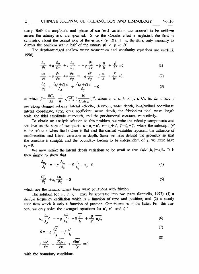
Considerable simplification can be achieved by taking the lateral depth variation to be exponential (Fig. 2), i.e., h=ae by (a and b are constants). Equation (13) then has constant coefficients
02( ' 02~ ' 0~' 0x 2 + ~ +2b ~ =Q(x,y) (16)
4 CHINESE JOURNAL OF OCEANOLOGY AND LIMNOLOGY Vol.16
and a Fourier series expansion can be applied oo
i ~ _ _ ( - Z B.sm(;~.x), (2. 2n - 1 .=l 2L
Variable channel depth
i r ..~ 0 2
1 0 , , ,
0 2 4 y(km)
n, n = 1, 2,'") (17)
This expansion satisfies the boundary condi- tions that ( '(x = 0)= 0, that the x - derivative of ~ at the head is zero, which is equivalent to ~ ( x = L ) = 0 . Using the other boundary condition ~ ' (y=0, D ) = 0 , the solution for B, can be shown to he
B. = e~2YK.(y) + c,.d ~v + c~d ~v (18)
where
kl=-b- k2=-b+4b +
I2=fi-*,Yq.(y )dy 2 .
G(Y) = --s x,y)sm(2~x)dx
Fig. 2 The depth pmf'tles used for calculation. The upper panel shows different depth profdes when the shoal depth is fixed. The lower panel shows the profiles when the charmel depth is fixed
The residual velocity depends on the solution, i.e. a/h o, L/2 and fl/(aho). In h.~n/h~..x, since
hmm 4- /(In h~. ) 2 _{_ ( _ _
kl,:/) =In h~ X/ hm~x
1 {k2ek#K.(D)+ek~I~ (D)} Cin-- k l ( d # _ d ~ )
kl C~- - k2 Cl.
dimensionless parameters in the first order addition, they also depend on D/L and
2 n - 1 D n)2 (19) 2 L
In the next section, discussion will be focused on the results of calculating ur, Vr and ~'.
THE STRUCTURE OF THE RESIDUAL FLOW
The solution in the previous section has shown that the residual circulation de- pends on five pamrmters: a/ho, L/2, h~n/h~x, D/L and fl/(aho). Calculations for the solution are made for various sets of parameters in the following range: a/ho=O.03-0.38 , L/2=0.014-1 , and h ~ / h ~ = 0 . 5 - 0 . 9 8 . The width to length ratio, D/L, turns out to have little effect on the residual circulation structure and the maxi- mum residual velocity.
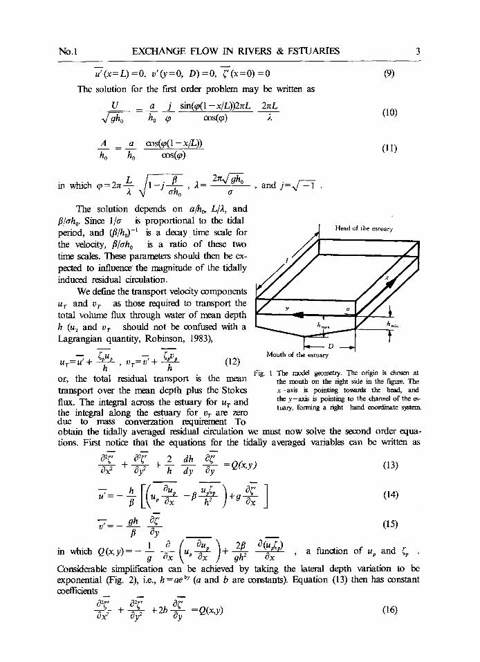
Figure 3 shows a distorted vector map of the residual transport velocity (u' and v ' , and D and L are not drawn proportionally), for the shoal depth = 5 m, channel depth = 10 in, half width = 2 kin, tidal amplitude at the mouth = 1 in. and the length of the estuary = 75 km. The estuary length is approximately 0.8 tixms one quarter of the tidal wave length. In this example, the m2tximum magnitude of the longitudinal component is two orders of magnitude ( ~ 11 cm/s) larger than the lateral component ( ~ 1.6 ram). The following characteristics are typical of our solutions: (1) the residual tmmport velocity mag-
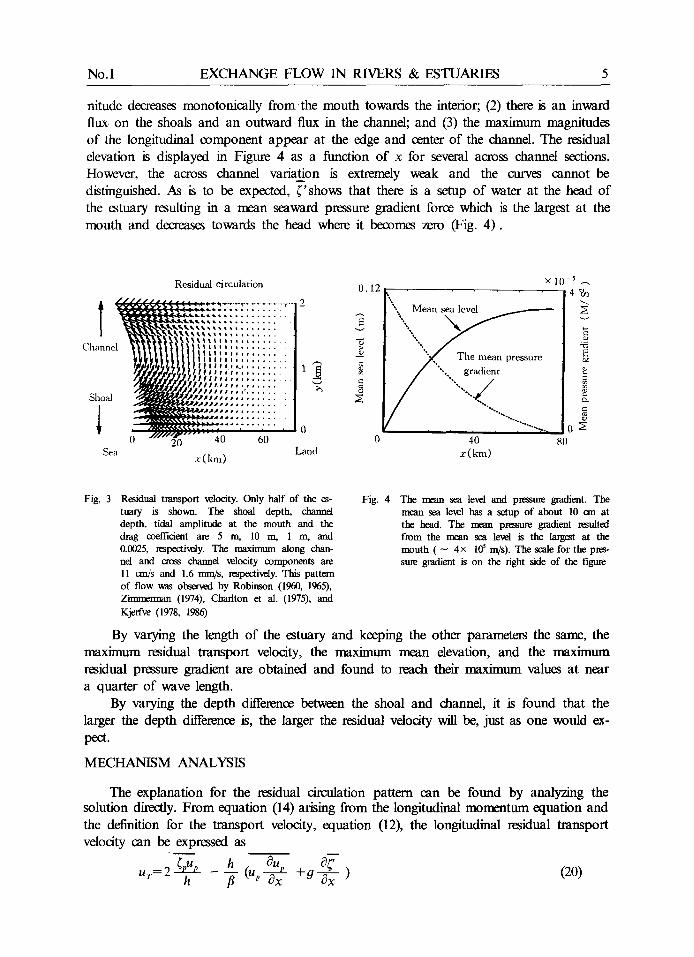
No.1 EXCHANGE FLOW IN RIVERS & ESTUARIES 5
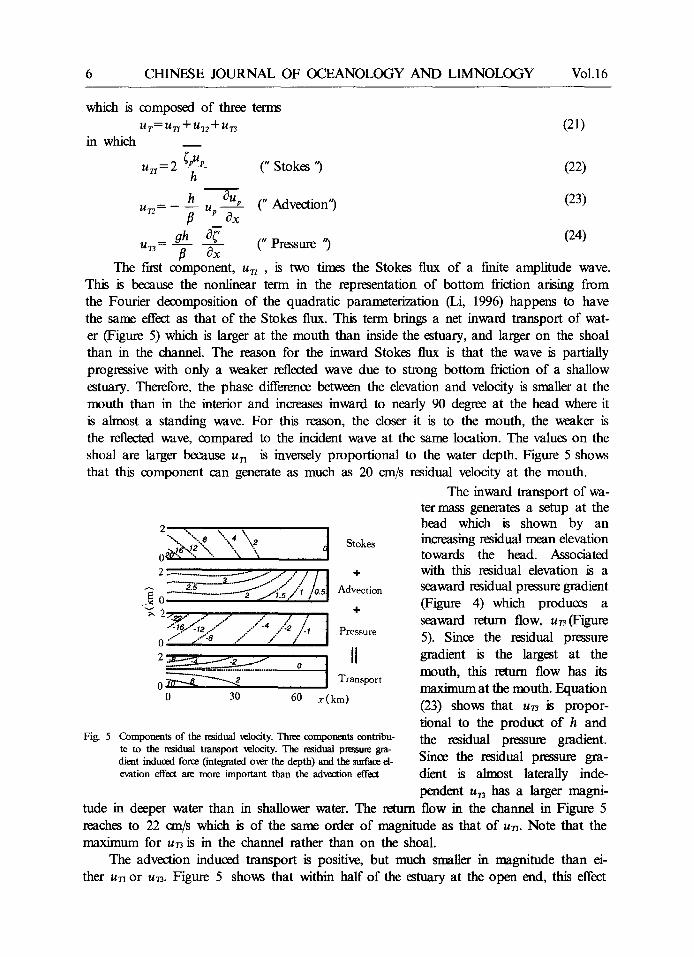
nitude decreases monotonically from the mouth towards the interior; (2) there is an inward flux. on the shoals and an outward flux in the channel; and (3) the maximum magnitudes of the longitudinal ~ m p o n e n t appear at the edge and center of the channel. The residual elevation is displayed in Figure 4 as a function o f x for several across channel sections. However, the across channel variation is extremely weak and the curves cannot be distinguished. As is to be expected, ~'shows that there is a setup of water at the head of the estuary resulting in a mean seaward pressure gradient force which is the largest at the mouth and decreases towards the head where it becomes zero (Fig. 4 ) .
Residual circulation 0.12
~ ~ ...........
fllllil'" . . . . . . . . . . . . I # # l d d d , ~ L L [ [ I | I I # I I ~ ~., , . . . . . . .
T t t l 4 r l ] ] Y . ? ) l t t t t ~ , , ..........
/ ~ t 1 1 1 1 1 1 ~ , , , ~ . . . . . . .
/ ~ ; I ~ t ~ H * , , , . . . . . . . . .
0 j///H.~.- . . . . . . 40 60
~: ( k m )
2
?
2O Sea Land x ( k m )
• 10 -5
I ~ . . . . . . . 4"0z
M e a n ~ v ~
" ' ~ , The mean pressure
/",,,,7 ..........
. . . . . . v~ 0 40 80
Fig, 3 Residual transport velocity. Only half of the es- tuary is shown. The shoal depth, channel depth, tidal amplitude at the mouth and the drag coefficient are 5 m, 10 m, 1 m, and 0.0025, resp~tively. The maximum along chan- nel and cross channel velocity components aie 11 cm/s and 1.6 ram/s, respectively. This pattern of flow was obser~d by Robinson (1960, 1965), Zimanemmn (1974), Chaflton et al. (1975), and Kjerfve (1978, 1986)
By varying the length of the estuary and keeping the other parameters the same, the maximum residual transport velocity, the maximum mean elevation, and the maximum residual pressure gradient are obtained and found to reach their maximum values at near a quarter of wave length.
By varying the depth difference between the shoal and channel, it is found that the larger the depth differenee is, the larger the residual velocity will be, just as one would ex- pect.
Fig. 4 The mean sea level and pressure gradient. The mean sea level has a setup of about 10 cm at the head. The mean pressure gradient resulted from the mean sea level is the largest at the mouth ( ~ 4x 10 5 m/s). The scale for the pr~- sure gradient is on the fight side of the figure
MECHANISM ANALYSIS
The explanation for the residual circulation pattern can be found by analyzing the solution directly. From equation (14) arising from the longitudinal momentum equation and the definition for the transport velocity, equation (12), the longitudinal residual transport velocity can be expressed as
u r = 2 ~up h Ou 0~' - - ( u p @ e- +O ) (20) h fl t,x
6 CHINESE JOURNAL OF OCEANOLOGY AND LIMNOLOGY Vol.16
which is composed of three terms
Ur= u~ + ur2 + u~ (21) in which
u ~ = 2 ~puv C Stokes ') (22) h
h up 0% C Advection') (23)
gh O~ 7 (" Pressure ") (24) u . - fl C~x
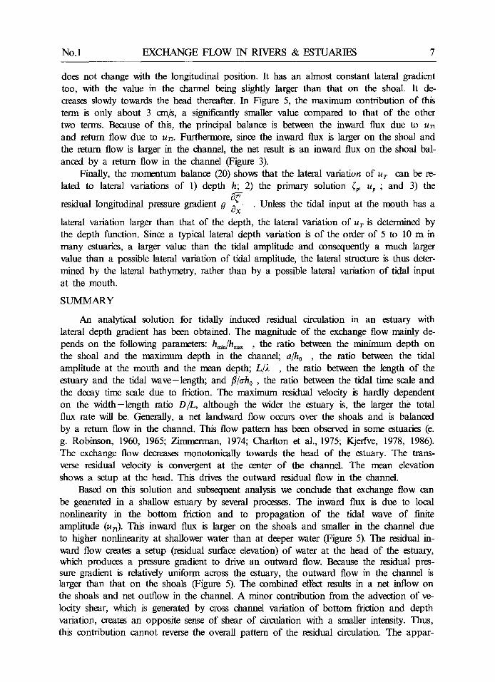
The first component, u~ , is two times the Stokes flux of a finite amplitude wave. This is because the nonlinear term in the representation of bottom friction arising from the Fourier decomposition of the quadratic parameterization (Li, 1996) happens to have the same effect as that of the Stokes flux. This term brings a net inward transport of wat- er (Figure 5) which is larger at the mouth than inside the estuary, and larger on the shoal than in the channel. The reason for the inward Stokes flux is that the wave is partially progressive with only a weaker reflected wave due to strong bottom friction of a shallow estuary. Therefore, the phase difference between the elevation and velocity is smaller at the mouth than in the interior and increases inward to nearly 90 degree at the head where it is almost a standing wave. For this reason, the closer it is to the mouth, the weaker is the reflected wave, compared to the incident wave at the same location. The values on the shoal are larger because un is inversely proportional to the water depth. Figure 5 shows that this component can generate as much as 20 cm/s residual velocity at the mouth.
mJ 2_~::::::::~___~i/5-..,.,.,..... / I !
2.5 ~ ~.:" . / i /o.51 0 ": , . I "%" { I
o ~ - - - ~ 4 0 30
Stokes
§
Advection
§
Pressure
II I Transport
60 x(km)
Fig. 5 Components of the residual velocity. Three oomponents contribu- te to the residual tramport velocity. The residual premure gra- dient induced force (integrated over the depth) and the surface el- evation effect are more important than the advection effect
The inward transport of wa- termass generates a setup at the head which is shown by an increasing residual mean elevation towards the head. Associated with this residual elevation is a seaward residual pressure gradient (Figure 4 )wh ich produces a seaward return flow, ur3(Figure 5). Since the residual pressure gradient is the largest at the mouth, this return flow has its maximum at the mouth. Equation (23) shows that u , is propor- tional to the product of h and the residual pressure gradient. Since the residual pressure gra- dient is almost laterally inde- pendent un has a larger magni-
tude in deeper water than in shallower water. The return flow in the channel in Figure 5 reaches to 22 cm/s which is of the same order of magnitude as that of u~. Note that the maximum for un is in the channel rather than on the shoal.
The advection induced transport is positive, but much smaller in magnitude than ei- ther un or un. Figure 5 shows that within half of the estuary at the open end, this effect
No.1 EXCHANGE FLOW IN RIVERS & ESTUARIES 7
does not change with the longitudinal position. It has an almost constant lateral gradient too, with the value in the channel being slightly larger than that on the shoal. It de- creases slowly towards the head thereafter. In Figure 5, the maximum contribution of this term is only about 3 cm/s, a significantly smaller value compared to that of the other two terms. Because of this, the principal balance is between the inward flux due to un and return flow due to u , . Furthermore, since the inward flux is larger on the shoal and the return flow is larger in the channel, the net result is an inward flux on the shoal hal- anced by a return flow in the channel (Figure 3).
Finally, the mormaatum balance (20) shows that the lateral variation of UT can be re- lated to lateral variations of 1) depth h; 2) the primary solution Cp, Up ; and 3) the
residual longitudinal pressure gradient g ~ . Unless the tidal input at the mouth has a
lateral variation larger than that of the depth, the lateral variation of UT is determined by the depth function. Since a typical lateral depth variation is of the order of 5 to 10 m in many estuaries, a larger value than the tidal amplitude and consequently a much larger value than a possible lateral variation of tidal amplitude, the lateral structure is thus deter- mined by the lateral bathyrnetry, rather than by a possible lateral variation of tidal input at the mouth.
SUMMARY
An analytical solution for tidally induced residual circulation in an estuary with lateral depth gradient has been obtained. The magnitude of the exchange flow mainly de- pends on the following parameters: h~i,/h,~x , the ratio between the minimum depth on the shoal and the maximum depth in the channel; a/ho , the ratio betwe~a the tidal ampfitude at the mouth and the mean depth; 1_./2 , the ratio between the length of the estuary and the tidal wave-length; and fl/aho , the ratio between the tidal time scale and the decay time scale due to friction. The maximum residual velocity is hardly dependent on the width-length ratio D/L, although the wider the estuary is, the larger the total flux rate will be. Generally, a net landward flow occurs over the shoals and is balanced by a return flow in the channel. This flow pattern has been observed in some estuaries (e. g. Robinson, 1960, 1965; Zimmerman, 1974; Charlton et al., 1975; Kjerfve, 1978, 1986). The exchange flow d~a'eases monotonically towards the head of the estuary. The trans- verse residual velocity is convergent at the center of the channel. The mean elevation shows a setup at the head. This drives the outward residual flow in the channel.
Based on this solution and subsequent analysis we conclude that exchange flow can be generated in a shallow estuary by several processes. The inward flux is due to local nonlinearity in the bottom friction and to propagation of the tidal wave of finite amplitude (un). This inward flux is larger on the shoals and smaller in the channel due to higher nonlinearity at shallower water than at deeper water (Figure 5). The residual in- ward flow creates a setup (residual surface elevation) of water at the head of the estuary, which produces a pressure gradient to drive an outward flow. Because the residual pres- sure gradient is relatively uniform across the estuary, the outward flow in the channel is larger than that on the shoals (Figure 5). The combined effect results in a net inflow on the shoals and net outflow in the channel. A minor contribution from the advection of ve- locity shear, which is generated by cross channel variation of bottom friction and depth variation, creates an opposite sense of shear of circulation with a smaller intensity. Thus, this contribution cannot reverse the overall pattern of the residual circulation. The appar-
8 CHINESE JOURNAL OF OCEANOLOGY AND LIMNOLOGY Vol.16
ent contradiction between the previous theory and observation, which has aready been re- cognized (Zimmerman, 1981) is due to the exclusion of nonlinear effects of fmite surface elevation which are much more important in shallow estuaries.
It is important to note that, although the present model is highly simplified, the rnechanisrns identified are independent of the simplifications. In a specific estuary, the ge- ometry will cause more complicated distributions of amplitudes for the incident and re- flected waves, and thus cause complicated distribution for the phase difference between the velocity and elevation of the tide, which will in turn affect the pattern of the exchange flow (Li, 1996). This increase of complexity, however, does not add more fundanaental mechanism to the process. Nevertheless, a challenge remains for the separation of the barotmpic flow from the baroclinic flow to further test this theory in real estuaries.
ACKNOWLEDGMENT
This work was supported by grants from the National Science Foundation(OCE 88616566), and The State of Connecticut Department of Environmental Protection Clean Water Fund (CWF 267R). Discussions with and/or suggestions from Prof. P. Bogden, and Prof. Munchow are appreciated. We are grateful to M. M. Howard-Strobel for allowing us to use her graphics software and for other help on numerous occasions.
Refermom
Charlton, J. A., McNicoU, W., West, J. R., 1975. Tidal and freshwater induced circulation in the Tay Estuary. Proc. R. Soc. Edinburgh B75:11-27.
Fi,w.her, H. B., 1972. Mass transport rrechanisms in partially stratified estuaries. J. Fluid Mech. 53 (4):671-687. Hamrick, J. M., 1979. Salinity intrusion and gravitational circulation in partially stratified estuaries. Ph.D. Dissertation,
U. of California, Berkeley, pp.451. Hansen, D.V. and Rattray, M., 1965: Gravitational circulation in straits and estuaries. J. Marine Res., 23: 104-22. lannieUo, J. P., 1977. Non-linearly induced r~idual currents in tidally dominated estuaries. Ph.D. dissertation, U. of
Connecticut, pp.250. Kjerfve, B., 1978. Bathymetry as an indicator of net circulation in v~ll mixed estuaries. Limnology and Oceanography,
23: 816- 821. Kjerfve, B., 1986. Circulation and salt flux in a ~/1 mixed estuary. In: Physics cf Sl~llow Estuaries and Bays, Coastal
Esttarine Stud., SpringerVeflag, Vol. 16: edited by J. van de Kreeke. pp. 22-29. Li, C., 1996. Tidally induced residual circulation in estuaries with cross channel bathymetry. Ph.D. dissertation,
U. of Connecticut, pp242. Pritchard, D.W., 1952. Salinity distribution and circulation in the Chesapeake estuarine system. J.. Mar. Re~, 11:
106-123. Robinson, A. H. W., 1960. Ebb- f lood ch~annel systems in sandy bays and estuaries. Geography, 45:. 183-199. Robinson, A. H. W., 1965. The use of the sea bed drifter in coastal studies with particular reference to the Humber. Z.
Geograph. Supplernentband 7 : 1 - 2 2 . Robinson, I. S., 1983. Tidally induced residual flow. Physical Oceanography of Coastal and Shelf Seas (B. Johns, ed.),
Elsevier, Amsterdam, 321-356. Research 2~ 195-212. Wong, K - C . , 1994. On the nature of transverse variability in a coastal plain estuary. J Geophy~ Res. 99(C7):
14209-14222. Zimmerman, J .T .F . , 1974. Circulation and water exchange near a tidal watershed in the Dutch Wadden Sea.
Netherlands J. o f Sea Re~ 8:126-138. Z i ~ , J. T. F., 1981. Dynamics, diffusion and geomorphological significance of tidal residual eddies. Nature 290:.
549- 555.


![Residual Tide analysis in shallow waTeR - …...Tidal analysis For the tidal analysis the classical least squares harmonic approach is preferred over the response method [7] – due](https://img.pdfslide.net/doc/110x75/5f387bd3163dad3d5169160b/residual-tide-analysis-in-shallow-water-tidal-analysis-for-the-tidal-analysis.jpg)