On the Milky Way Haze and Dark Matter

Elena Pierpaoli (Univ. of Southern California)

Andrey Egorov (USC), Davide Pietrobon (Berkely), Jennifer Gaskins (Univ. of Amsterdam)

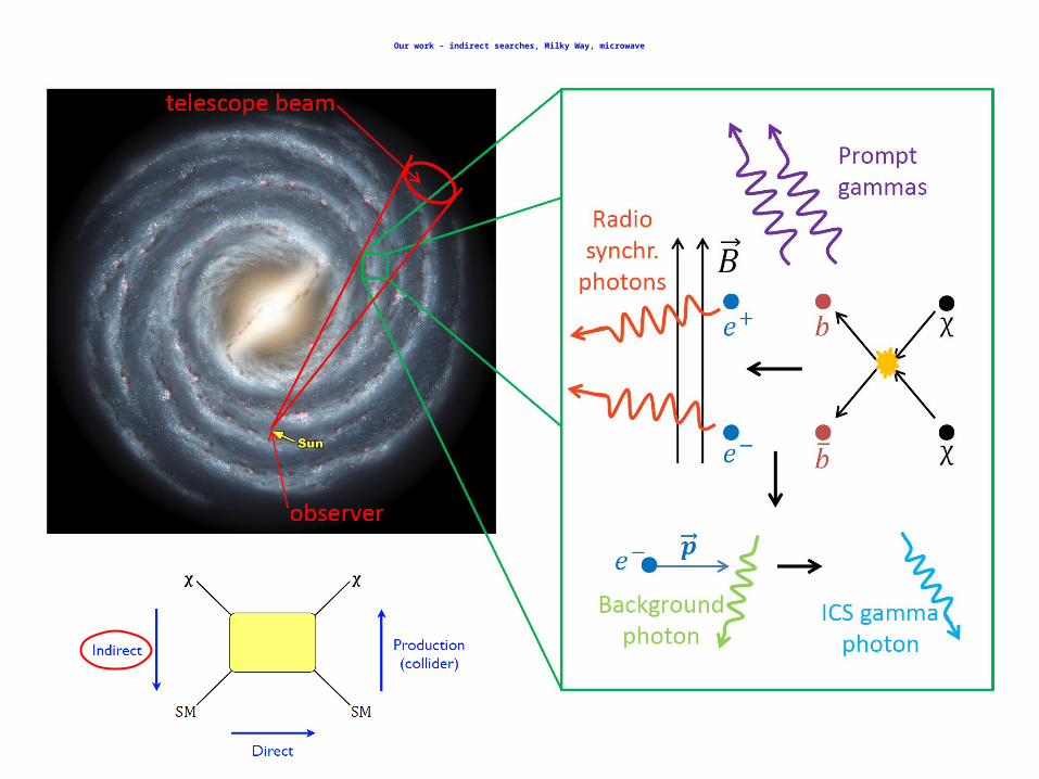
O u r w o rk – in d ire ct se arch e s, M ilky W ay, m icro w ave

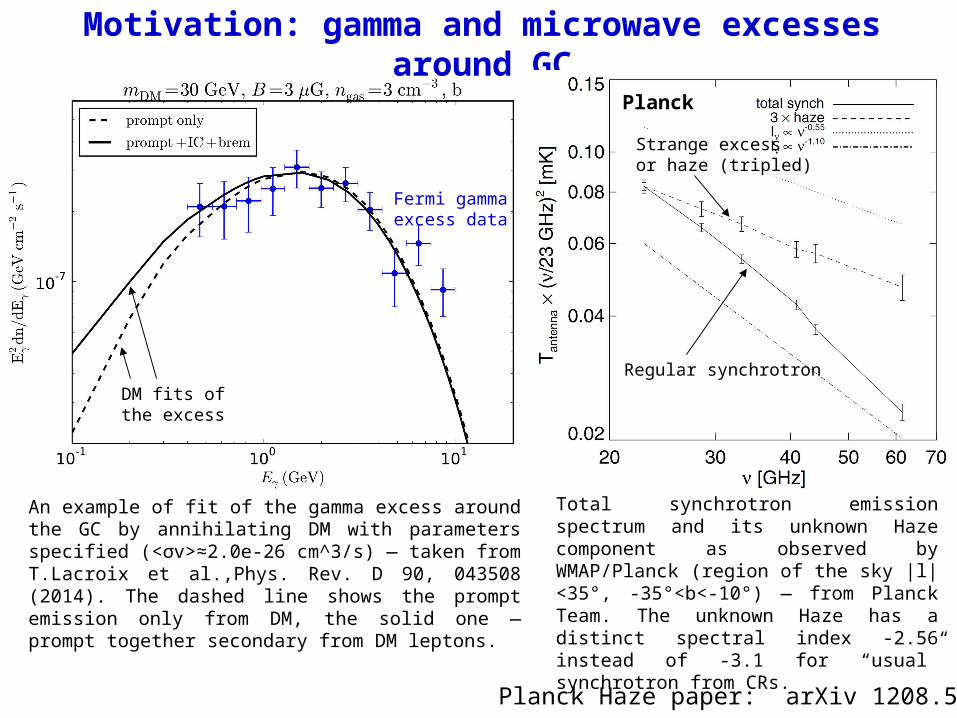
Motivation: gamma and microwave excesses around GC

An example of fit of the gamma excess around the GC by annihilating DM with parameters specified (<σv>≈2.0e-26 cm^3/s) — taken from T.Lacroix et al.,Phys. Rev. D 90, 043508 (2014). The dashed line shows the prompt emission only from DM, the solid one — prompt together secondary from DM leptons.

Total synchrotron emission spectrum and its unknown Haze component as observed by WMAP/Planck (region of the sky |l|<35°, -35°<b<-10°) — from Planck Team. The unknown Haze has a distinct spectral index -2.56 instead of -3.1 for “usual” synchrotron from CRs.

Fermi gammaexcess data

DM fits of the excess

Planck

Regular synchrotron

Strange excess or haze (tripled)

Planck Haze paper: arXiv 1208.5483

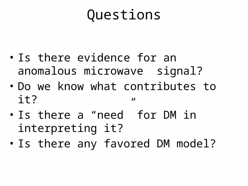
Questions

• Is there evidence for an anomalous microwave signal?

• Do we know what contributes to it?• Is there a “need” for DM in interpreting it?• Is there any favored DM model?

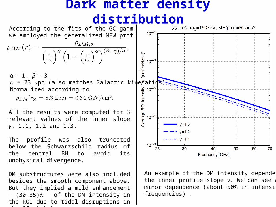
Dark matter density distributionAccording to the fits of the GC gamma excess,we employed the generalized NFW profile:

α = 1, β = 3rs = 23 kpc (also matches Galactic kinematics)Normalized according to

All the results were computed for 3 relevant values of the inner slope γ: 1.1, 1.2 and 1.3.

The profile was also truncated below the Schwarzschild radius of the central BH to avoid its unphysical divergence.

DM substructures were also included besides the smooth component above. But they implied a mild enhancement – (30-35)% - of the DM intensity in the ROI due to tidal disruptions in the GC vicinity.

An example of the DM intensity dependence onthe inner profile slope γ. We can see a relatively minor dependence (about 50% in intensity at all frequencies) .

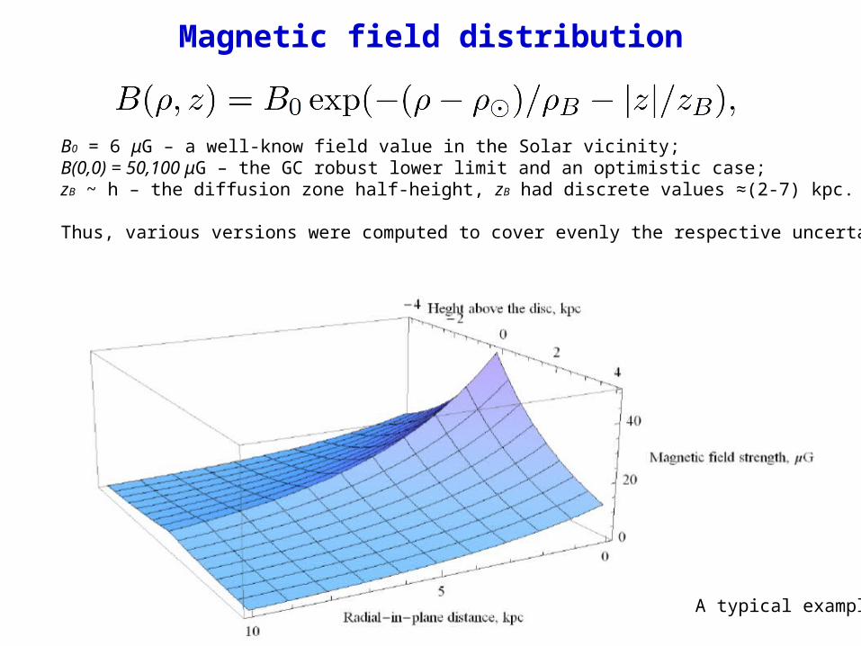
Magnetic field distribution

B0 = 6 μG – a well-know field value in the Solar vicinity;B(0,0) = 50,100 μG – the GC robust lower limit and an optimistic case;zB ~ h – the diffusion zone half-height, zB had discrete values ≈(2-7) kpc.

Thus, various versions were computed to cover evenly the respective uncertainty range.

A typical example.

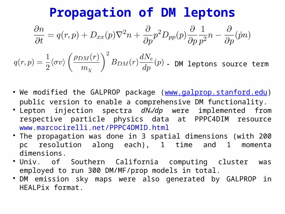
Propagation of DM leptons

- DM leptons source term

We modified the GALPROP package (www.galprop.stanford.edu) public version to enable a comprehensive DM functionality.

Lepton injection spectra dNe/dp were implemented from respective particle physics data at PPPC4DIM resource www.marcocirelli.net/PPPC4DMID.html

The propagation was done in 3 spatial dimensions (with 200 pc resolution along each), 1 time and 1 momenta dimensions.

Univ. of Southern California computing cluster was employed to run 300 DM/MF/prop models in total.

DM emission sky maps were also generated by GALPROP in HEALPix format.

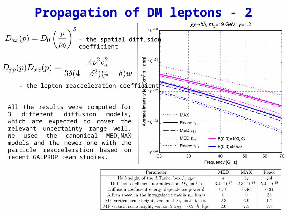
Propagation of DM leptons - 2

- the spatial diffusioncoefficient

- the lepton reacceleration coefficient

All the results were computed for 3 different diffusion models, which are expected to cover the relevant uncertainty range well. We used the canonical MED,MAX models and the newer one with the particle reacceleration based on recent GALPROP team studies.

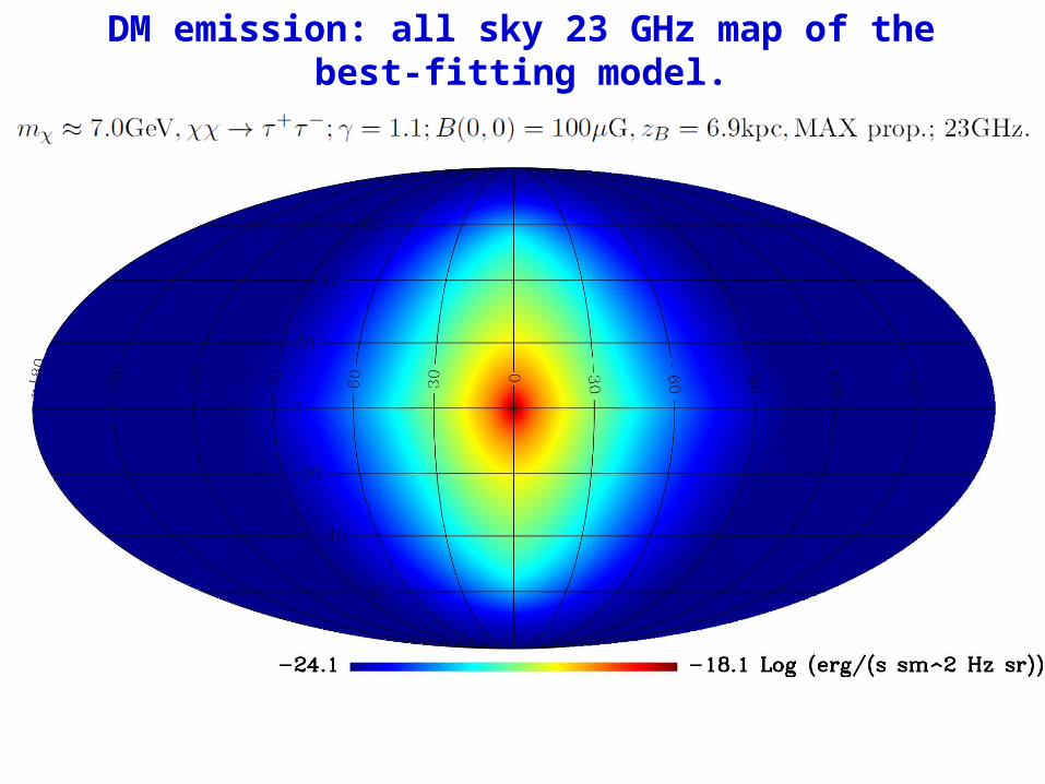
DM emission: all sky 23 GHz map of the best-fitting model.

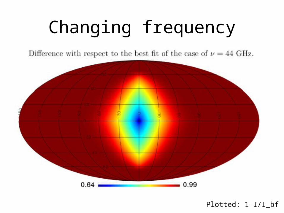
Changing frequency

Plotted: 1-I/I_bf

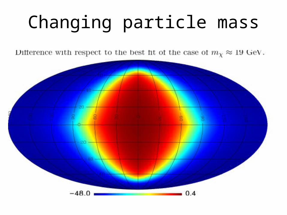
Changing particle mass

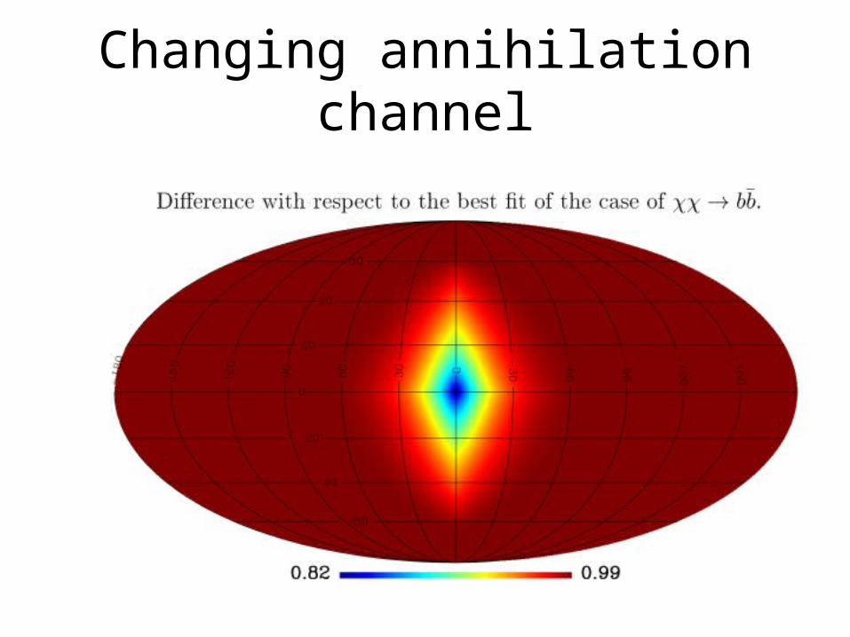
Changing annihilation channel

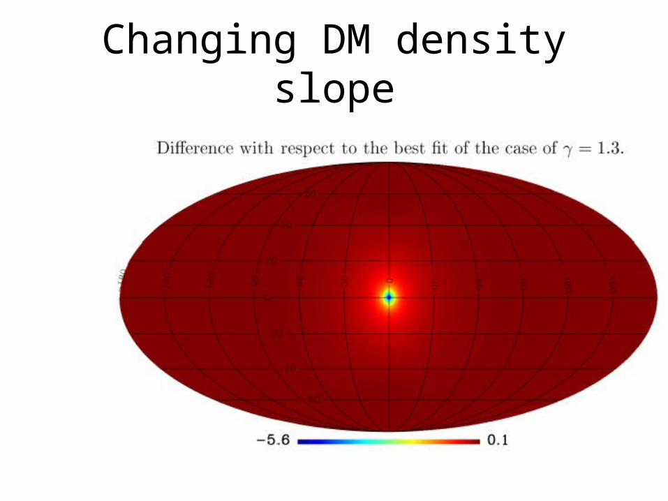
Changing DM density slope

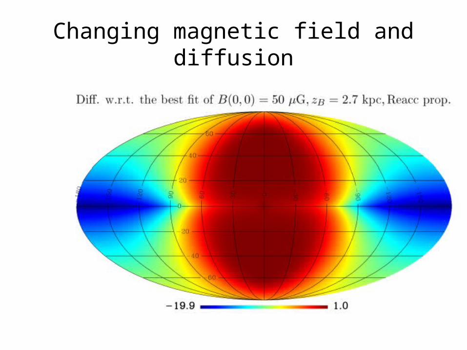
Changing magnetic field and diffusion

Procedures applied

• METHOD I: Conservative estimate: Overall upper limit to the DM signal (ignoring foregrounds and considering only the CMB)

• METHOD II: Less conservative estimate: Template fitting procedure (therefore including foreground subtraction) – results depend on assumptions on foregrounds and specific method adopted.

• Intermediate step: single frequency fitting.

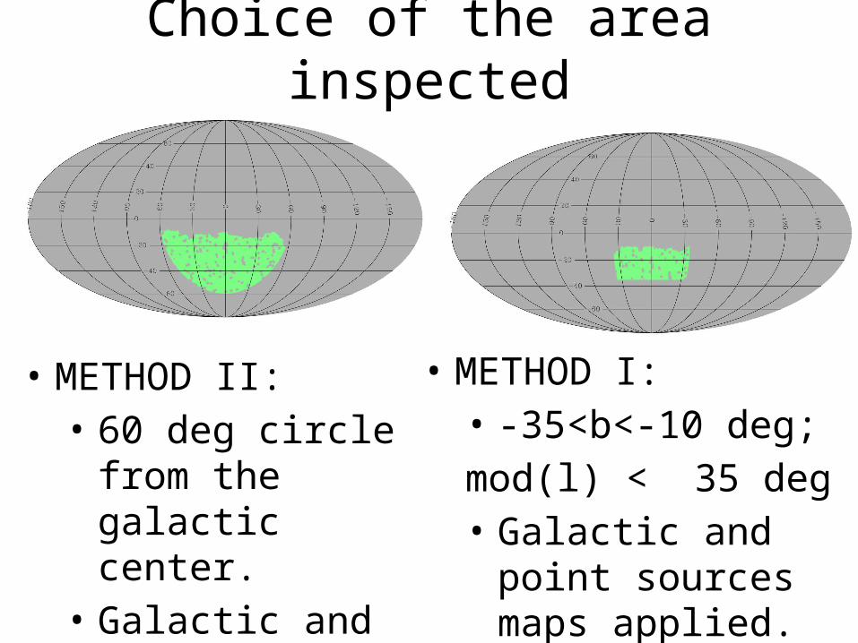
Choice of the area inspected

• METHOD II:• 60 deg circle from

the galactic center.• Galactic and point

sources maps applied.

• METHOD I:• -35<b<-10 deg;mod(l) < 35 deg• Galactic and point

sources maps applied.

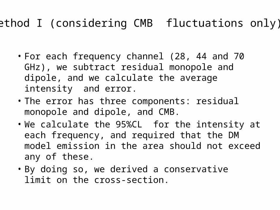
Method I (considering CMB fluctuations only)

• For each frequency channel (28, 44 and 70 GHz), we subtract residual monopole and dipole, and we calculate the average intensity and error.

• The error has three components: residual monopole and dipole, and CMB.

• We calculate the 95%CL for the intensity at each frequency, and required that the DM model emission in the area should not exceed any of these.

• By doing so, we derived a conservative limit on the cross-section.

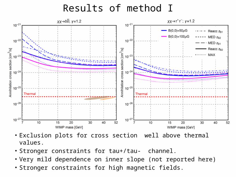
Results of method I

• Exclusion plots for cross section well above thermal values.• Stronger constraints for tau+/tau- channel.• Very mild dependence on inner slope (not reported here)• Stronger constraints for high magnetic fields.

Method II (with foreground subtraction) • Multi-frequency template fitting of:

– CMB [ILC map from HFI channels]– Free-free [H_alpha map]– Synchrotron [Haslam 408MHz]– Dust [SFD]– “Bubbles”

• MCMC (assuming Gaussian Likelihood) to derive amplitudes of the various components, without assuming a frequency dependence for any (aside from CMB and the DM one)

• DM maps for each model and frequency computed with GALPROP.

• Data: 4 WMAP (23,33,41,61 GHz) and 3 Planck LFI (23, 44, 70 GHz) 2013 temperature maps.

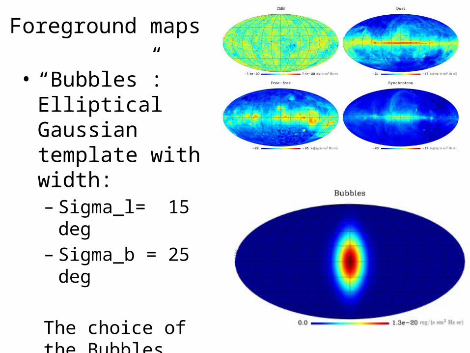
Foreground maps

• “Bubbles”: Elliptical Gaussian template with width: – Sigma_l= 15 deg – Sigma_b = 25 deg

The choice of the Bubbles component matches Dobler et al 2012

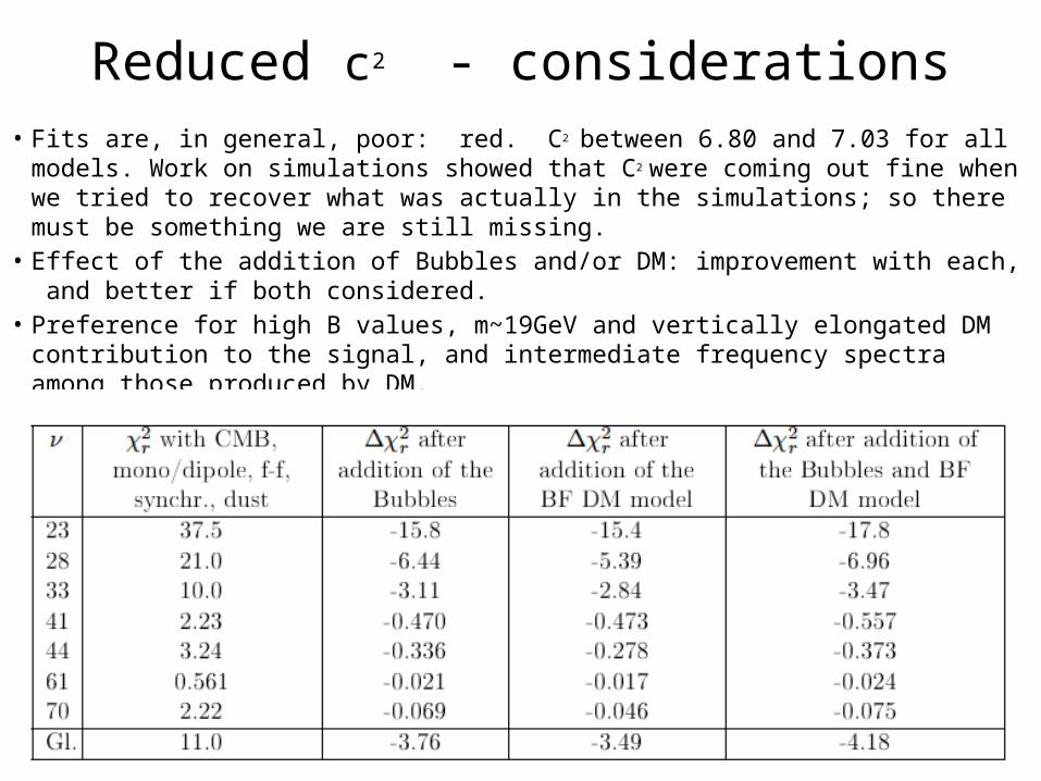
Reduced c2 - considerations• Fits are, in general, poor: red. C2 between 6.80 and 7.03 for all models. Work on

simulations showed that C2 were coming out fine when we tried to recover what was actually in the simulations; so there must be something we are still missing.

• Effect of the addition of Bubbles and/or DM: improvement with each, and better if both considered.

• Preference for high B values, m~19GeV and vertically elongated DM contribution to the signal, and intermediate frequency spectra among those produced by DM.

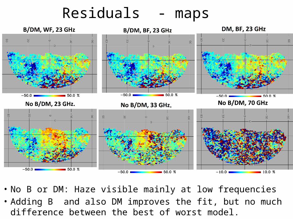
Residuals - maps

• No B or DM: Haze visible mainly at low frequencies• Adding B and also DM improves the fit, but no much difference between

the best of worst model.

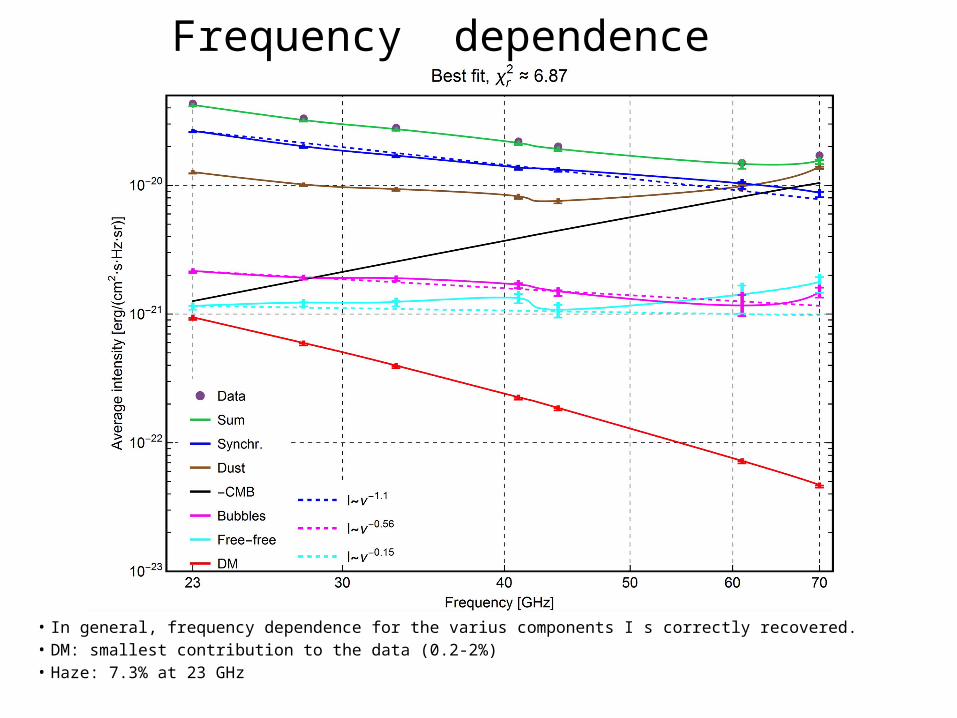
Frequency dependence

• In general, frequency dependence for the varius components I s correctly recovered.• DM: smallest contribution to the data (0.2-2%)• Haze: 7.3% at 23 GHz

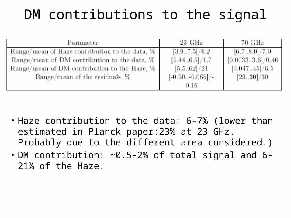
DM contributions to the signal

• Haze contribution to the data: 6-7% (lower than estimated in Planck paper:23% at 23 GHz. Probably due to the different area considered.)

• DM contribution: ~0.5-2% of total signal and 6-21% of the Haze.

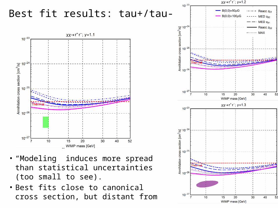
Best fit results: tau+/tau-

• “Modeling” induces more spread than statistical uncertainties (too small to see).

• Best fits close to canonical cross section, but distant from

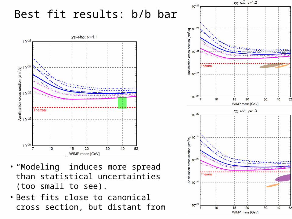
Best fit results: b/b bar

• “Modeling” induces more spread than statistical uncertainties (too small to see).

• Best fits close to canonical cross section, but distant from

Conclusions

• The Haze exists (6-7% of the total signal at 23 GHz) and it has a harder spectrum than usual synchrotron.

• Data do not show a preference in fitting the Haze with Bubble or DM. Both produce improvements.

• When both included, best fit model has 20-30% of Haze explained by DM.

• Some DM model preferred to others. The preferred WIMP cross section does not match those of the gamma-ray excess.

• The thermal cross-section, as well as gamma-ray derived cross-sections, are within the most conservative estimates found with Planck maps.