Computer Science Department

TECHNICAL REPORT

On the 'Piano Movers' ProblemII. General Techniques for Computing

Topological Properties of RealAlgebraic Manifolds

Jacob T. Schwartz

AND

Micha Sharir

February I982

NEW YORK UNIVERSITY

Department of Computer Science

Courant Institute of Mathematical Sciences

251 MKRCKR STREET, NEW YORK, N.Y. 10012

On the 'Piano Movers' ProblemII. General Techniques for Computing

Topological Properties of RealAlgebraic Manifolds

BY

Jacob T. Schwartz

AND

Micha Sharir

February 1982Report No. ^1

y^'Lf I

This work has been supported in part by ONR Grant N0001^-75-C-0571

,

by NSF Grant MCS-80-Oi^3^9, and by U.S. Doe Office of Energy ResearchContract Ey-76-C-o2-3077

.

r .'

On the 'Piano Movers' Problem

II, General Techniques for Computing Topological Properties of Real

Algebraic Manifolds ^*^

Jacob T. SchwartzComputer Science Department

Courant Institute of Mathematical Sciences

and

Micha SharirDepartment of Mathematical Sciences

Tel Aviv University

ABSTRACT; This paper continues the discussion, begun in [SS], of thefollowing problem, which arises in robotics: Given a collection of

bodies B, which may be hinged, i.e. may allow internal motion aroundvarious joints, and given a region bounded by a collection ofpolyhedral or other simple walls, decide whether or not there exists a

continuous motion connecting two given positions and orientations of

the whole collection of bodies. We show that this problem can behandled by appropriate refinements of methods introduced by Tarski andCollins, which lead to algorithms for this problem which are polynomialin the geometric complexity of the problem for each fixed number of

degrees of freedom (but exponential in the number of degrees of

freedom.) Our method, which is also related to a technique outlined by

Reif, also gives a general (but not polynomial-time) procedure forcalculating all of the homology groups of an arbitrary real algebraicvariety. Various algorithmic issues concerning computations withalgebraic numbers, which are required in the algorithms presented inthis paper, are also reviewed.

(*) Work on this paper has been supported in part by the Office ofNaval Research Contract N00014-75-C-0571 ; Work by the second author hasalso been supported in part by the Bat-Sheva Fund at Israel.

-2-

0. Introduction

The 'Piano Movers' problem (see [Re], [LPW], [IKP], [Ud] , [SS]) is

that of finding a continuous motion which will take a given body or

bodies B from a given initial position to a desired final position, but

which is subject to certain geometric constraints during the motion.

These constraints forbid the bodies to come in contact with certain

obstacles or 'walls', or to collide with each other. These walls can,

be curved, and the full collection of walls is not required be

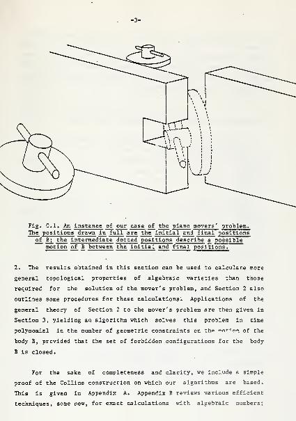
connected (see Fig. 0.1). The problem that we set out to solve is:

Given two configurations (i.e. positions and orientations of all

subparts) of the bodies B in which none of these bodies touches any

walls, and in which none of the bodies B collide, find a continuous

wall- and collision-avoiding motion of all the B between these two

configurations, or establish that no such motion exists.

This paper will present a general, though not very efficient,

method for deciding on the existence of such a path (and for

constructing such a path if it exists). Specifically, we will show

that this problem can be handled by a variant of Tarski's famous

algorithm [Ta] for deciding statements in the quantified elementary

theory of real numbers. Our approach is related to that outlined in an

interesting paper of Reif [Re], and makes essential use of technical

devices introduced by Collins [Co] and reviewed by Arnon [Ar] . As we

shall see, these techniques also allow explicit, constructive

calculation of the homology groups of an arbitrary real algebraic

variety. In particular, the connectivity of such a variety can be

calculated easily.

The paper is organized as follows. In Section 1 we begin to

formulate the general mover's problem in which we are interested, as an

abstract computational problem in algebraic topology. The algebraic

mechinery required to handle this problem is then developed in Section

3-

Fig. 0.1. An Instance of our case of the piano movers' problem.The positions drawn in full are the initial and final positions

of B; the intermediate dotted positions describe a_ possiblemotion of B between the initial and final positions.

2. The results obtained in this section can be used to calculate more

general topological properties of algebraic varieties than those

required for the solution of the mover's problem, and Section 2 also

outlines some procedures for these calculations. Applications of the

general theory of Section 2 to the mover's problem are then given in

Section 3, yielding an algorithm which solves this problem in time

polynomial in the number of geometric constraints on thp "o'--'on of the

body B, provided that the set of forbidden configurations for the body

B is closed.

For the sake of completeness and clarity, we include a simple

proof of the Collins construction on which our algorithms are based.

This is given in Appendix A. Appendix B reviews various efficient

techniques, some new, for exact calculations with algebraic numbers;

such calculations appear repeatedly in our algorithms. Finally,

Appendix C gives technical details concerning the computations required

to obtain the topological structure of the Collins decomposition. Note

however that these, possible very expensive, computations are not

required for the simpler task of determining the connectivity of the

space of free configurations of the body B.

1. An Algebraic Formulation of the General Mover's Problem

In this section we reformulate the general motion-planning problem

in abstract algebraic terms, and reduce it to the problem of

decomposing certain algebraic varieties into their connected

components. A solution to this abstract problem is then developed in

subsequent sections.

Like Reif, whose work is to be presented more fully in a

forthcoming paper, we study the space of all collision-free positions

of one or more hinged bodies B. We assume each body B to consist of a

finite number of rigid compact subparts Bj^,B2,.., each bounded by

various algebraic surfaces. These subparts can be connected to each

other by various types of attachments, including the following:

(a) A point X on one part Bj can be fastened to a point Y on another

part B2, in a manner which requires X and Y to be coincident but does

not otherwise constrain the relative orientations of Bi and B2.

(b) The connection between X on Bj^ and Y on B2 can be a 'hinge', i.e.

can constrain B2 to revolve around an axis V fixed in the frame of B^.

(c) The connection between B^ and B2 can permit B2 to slide, or to

Various other forms of affixment might be envisaged and can be

treated in much the same way that we will treat the more common

fastenings (a-c) . As noted above, we are willing to consider any

number of disjoint hinged bodies of this kind, which are to move in a

coordinated fashion throughout an empty space bounded by a finite

collection of walls, which can themselves be arbitrary algebraic

surfaces. We can regard the walls as part of the given system of

bodies, with the additional properties that (a) they need not be

compact; and (b) they are constrained not to move at all.)

Since we intend to proceed algebraically in what follows, our

first task is to set up an appropriate algebraic parametrisation of a

superspace of the set of all allowed positions of the hinged body B. It

is convenient to proceed as follows. If B = B^ is a single rigid body,

we describe its position by giving a Euclidean motion T which takes B

from some standard position to its given position. This transformation

Tx «= Rx+Xq is defined by a pair [Xq,R] consisting of a point Xq in

3-dimensional Euclidean space E'^ and of a 3 by 3 rotation matrix R, and

can therefore be regarded as a point in a smooth six-dimensional1 -o

algebraic submanifold G of 12-dimensional Euclidean space E .

Next suppose that B is hinged, and that a second part B2 of B is

attached to Bi, say for the sake of definiteness in the manner (a).

Then we can describe the overall position of the two parts Bj^, B2 of B

as follows. As above, the position of Bj is described by a Euclidean

motion T which takes B, from a standard position to its actual

position. By applying the inverse T~ of T to both B, and B2, we put

Bj into its standard position, and B2 into a position which attaches a

fixed one of its points X2 to a point fixed on Bi. This position of B2

is therefore defined by giving a Euclidean transformation T2 such that

T2X2 " X2. It is plain that the set of these transformations is in 1-1

correspondence with the set of rotation matrices R2. Hence the overall

position of Bj and B2 can be represented by a pair [T,R2], which once

again varies over a smooth algebraic submanifold G2 of a

higher-dimensional Euclidean space E.

-6-

If instead B2 Is connected to B^ in the manner (b), then much the

same remarks apply, except that in this case the rotation matrix R2

must satisfy R2V - V for a certain 3-dimensional vector V. If B2 can

slide along an axis U fixed in B^ but not rotate, its position is

defined by a single real parameter u which defines the position of B2

along this axis, etc. In all cases, the overall position of B^ and B2

is described by a pair [12,12] of Euclidean motions, the first

unconstrained, the second confined to some subgroup of the full

Euclidean group. In all cases the allowed pairs form a smooth

algebraic submanifold G2 of some Euclidean space.

We can proceed similarly even if B consists of many parts hinged

together in various ways. Suppose, for example, that B2 is connected

to Bj, and that a third part B3 of B is connected to B2. Then as above

the overall position of Bj and B2 is defined by a pair [12,12] of

Euclidean transformations. T^ maps Bj from its standard to its actual

position, and T2T2 maps B2 from its standard to its actual position.

If we apply the inverse of 7^12 to B3, ^i put it into a position in

which it is attached to a fixed point or axis of B2 in one of the

manners (a-c). Hence the actual position of B2 is defined by a third

Euclidean transformation T^, belonging to a group of motions of one of

the types we have already considered, and the mapping T2T2T3 takes B3

from its standard to its actual position.

These considerations make it clear that, irrespective of the

manner in which the parts of a hinged body are connected together, the

overall position of all its parts can always be defined by a point

belonging to a smooth algebraic manifold G lying in a Euclidean space

of some appropriate dimension.

Of course, the preceding considerations ignore all restrictions on

the position of the parts of the bodies B imposed by the condition that

none of these parts must collide. This point will be handled in

Section 3 below, after the necessary algebraic machinery is introduced

and developed in Section 2, which now follows.

-7-

2. Tarski Sentences and Sets; The Collins Decomposition

By a Tarskl sentence we mean a sentence, possibly containing free

variables, which can be formulated In the decldable qxiantlfled language

studied by Tarskl [Ta]. In this language, variables designate real

numbers and are quantified over the set of all reals. The operators

allowed in the language are +, -, *, and /, designating the usual real

arithmetic operators. The allowed comparators are =,*,>, <, >, <,

all of which have their standard meanings. In addition quantifiers and

Boolean connectives are allowed.

A Tarskl sentence Q(xj x^) containing the indicated n free

variables and no others defines a subset of n-dimensional Euclidean

space E^, namely

(1) Iq= {[xi,...,x^]: Q(xi,...,x^)}.

Sets of this form will be called Tarskl sets (also known as

semi-algebraic sets ); the Q occurlng in (1) is called the defining

formula of Iq. By a result given in the cited paper of Tarskl, every

Tarskl set has a quantifier-free defining formula. A useful

constructive proof of this result, involving a penetrating analysis of

the geometric structure of Tarskl sets, is given by Collins [Co] (see

also Arnon [Ar]), and we will base our analysis of the general mover's

problem on Collins' results, which substantially improve Tarskl 's

earlier work. We will also prove certain topological properties of the

'cells' appearing in Collins' work, and will use these topological

Improvements to show that many standard topological properties (i.e.

all the homology groups) of any algebraic variety are effectively

calculable.

Using slightly different terminology than ours, Collins gives the

following definitions and theorems:

Definition 1: For any subset X of Euclidean space, a decomposition of X

is a finite collection K of disjoint connected subsets Y of X whose

-8-

union is X. Such a decomposition is a Tarski decomposition if each such

subset Y is a Tarski set.

In what follows, E^ will denote the Euclidean space of r

dimensions.

Definition 2; A cylindrical algebraic decomposition of E'^ is defined as

follows. For r=l such a decomposition is just a partitioning of E

into a finite set of algebraic numbers and into the finite and infinite

open intervals bounded by these numbers. For r > 1, a cylindrical

algebraic decomposition of E^ is a decomposition R obtained recursively

from some cylindrical algebraic decomposition K' of E^~^ as follows.

Regard E^ as the Cartesian product of E'^"^ and E , and accordingly

represent each point p of E^ as a pair [x,y] with x e E^"'^ and y e E .

Then K must be defined in terms of K' and an auxiliary polynomial P =

P(x,y) with rational coefficients, in the following way.

(i) For each c e K' , let c x E^ designate the cylinder over c, i.e.

the set of all [x,y] such that x e c.

(ii) For each c e K' there must exist an integer n, such that for each

X E c there are exactly n distinct real roots f^ (x) , . . . ,f ^^Cx) of P(x,y)

(regarded as a polynomial in y) , and hence these roots must vary

continuously with x. We suppose in what follows that these roots have

been enimerated in ascending order. Then each one of the cells of K

which intersects c x E^ must have one of the following forms:

(ii.a) {[x,y]: x e c, y < f,(x)}

(lower semi-infinite 'segment' of c x E^).

(ii.b) {[x,fi(x)]: X e c}

(ii.c) {[x.y]: X e c, fi(x) < y < fi+i(x)}

('segment' of c x E )

-9-

(ii.d) {[x,y]: X e c, f^U) < y}

(upper semi-infinite 'segment' of c x E^).

All these cells are said to have c as their base cell in K'; K' is said

to be the base decomposition , and P the base polynomial , of K. It is

convenient to put fgCx) = -« and f„+! (x) = +», and then to designate

the cells (ii.a), (ii.b), (ii.c), and (ii.d) as Cq*, c^, c^*, and c/respectively.

It obviously follows by induction that each of the sets

constituting a cylindrical algebraic decomposition K of E*" is

topologically equivalent to an open cell of some dimension k < r. We

will therefore refer to the elements c e K as the (open) Collins cells

of the decomposition K.

Definition 3: Let S be a set of functions of r variables, and K a

cylindrical algebraic decomposition of E^. Then K is said to be

S-invariant if, for each c in K and each f in S, one of the following

conditions holds uniformly for x e c: either

(a) f(x) = for all x e c; or

(b) f(x) < for all x e c; or

(c) f(x) > for all x e c.

Definition U: A point p e E^ is algebraic if each of its coordinates is

a real algebraic number. A defining polynomial for pis a polynomial

with rational coefficients whose set of roots includes all the

coordinates of p.

Theorem 1

:

(Collins) Given any finite set S of polynomials with

rational coefficients in r variables, we can effectively construct an

S-invariant cylindrical algebraic decomposition K of E^ into Tarski

sets such that each c e K contains an algebraic point. Moreover,

defining polynomials for all these algebraic points, and

quantifier-free defining formulae for each of the sets c e K, can also

be constructed effectively.

-10-

The proof of Collins' Theorem, which is not difficult, will be

reviewed in Appendix A below.

In what follows we will find it useful to sharpen Collins' results

in certain topological respects. For this, we have to impose an

additional requirement on the decomposition; in certain unfavorable

orientations of E^, this condition can be false. However, as we shall

show below, one can always restore this extra property by an

appropriate rotation of the r-Euclidean space, and such a rotation can

be easily calculated. This requirement is stated in the following

Definition 5: A Collins decomposition K is said to be well-based if the

following condition holds. Let K' be the base decomposition and P(b,x)

the base polynomial of K. Then we require that P(b,x) should not be

identically zero for any b e E'^"^. Moreover, we require that this same

condition apply recursively to the base decomposition K'

.

Example; Consider the polynomial

P(x,y,z) = (x2+y2)z + (x^-y^)

in 3-dimensional space E^. Then, since P(0,0,z) vanishes identically,

no P-invariant Collins decomposition of E*^ whose final step projects E"^

onto E'^ in the z-direction is well-based.

For the correctness of the topological assertions that we are

about to make, it is essential that the decomposition K be well-based.

Later we shall see how to rotate the given Euclidean space so as to

make the decomposition well-based. For the moment we assume a

well-based decomposition K, and show that it has certain useful

topological properties.

Lemma 1: Let c c K. Then the closure of r_is a union of cells of K.

Proof: To establish the lemma, we will use induction on the dimension

r, and prove the following stronger

-11-

Claim: Let r > 1, and let K be a Collins decomposition of E'^. Then the

closure of each cell in K is a union of cells of K. Moreover, for each

cell c of K, each point z in the boundary of c, and each e > 0, the

open c-ball about z contains a (relative) neighborhood U of z in c+{z}

such that U-{z} is a connected subset of c.

Proof of Claim: Our claim holds trivially for r = 1. Assume r > 1. With

no loss of generality assume that c has either the form

(1) c = Cj'* = { [b,x] : b e c', fj(b) < x < fj+i(b) },

(2) c = Cj' = { [b,fj(b)] : b e c' }.

for Some c' e K' = the base decomposition of K. In either case the

closure of c obviously contains c itself, and, in case (1), also the

two 'sections' c.' and c^^i' bounding c from above and from below, all

of which are of course cells in K. Any other point in the closure of c

must be of the form [b,x], where b belongs to the boundary of c', and

where Xi(b) < x < xoCb); here we write

xi(b) = lim inf fj(t') and X2(b) = lim sup ^k^^'^

b'ec', b'-^b b' ec' , b' + b

where k = j+1 in case (1), k = j in case (2). Conversely, any such

point clearly belongs to the closure of c. Let e be the set of all such

points. By our induction hypothesis, the boundary of c' is a union of

cells in K'. Let c'' e K' be a cell of this boundary. Note that Xj(b)

and X2(b) are either roots of P, or are -" or +". We will show that

these functions are (equal if k = j, and) continuous in the entire

closure of c, and hence are continuous for bee" (here we give the

extended real axis R* , including the points -<», -H», its standard

topology, which makes R homeomorphic to the compact unit interval

[-1.+1].)

, . -12-

The asserted continuity is an easy consequence of the following

auxiliary lemma.

Lemma 2; Let c' e K' be as above, and let fj(b) denote the j-th root of

P(b,») for bee'. Then -there exists a unique continuous extension (in

the sense of the extended topology of R ) of f ^ to the entire closure

of the cell c' . Moreover, this extension, which we will also denote by

f^, is either infinite or else a root of P.

It will be shown below that Lemma 2 follows inductively from our other

assertions. Assume for the moment that this has been proved. It then

follows that the set

K(c") = { [b,x] : b e c" , x^Cb) < x < X2(b) }

must be a union of cells in K. We can show this, and even provide a

more explicit characterization of these cells, as follows. Let c' e K'

be as above, and let f 4(b) be the j-th root (of m distinct real roots)

of P(b, •) over c' . Let c'' c K' be any cell in the boundary of c'.

Use the same symbol f^(b) to denote the continuous extension of f • to b

e c" which exists by Lemma 2. Then it follows from Lemma 2 that, for b

E c'', f^(b) is (either -"» or +» or) one of the M roots of P over c' '

.

In either case we can write f .(b) = Fj(b), where Fj is the J-th root of

P over c'' (by our convention, this also includes the extreme cases J =

0,M+1); note that J is independent of b, because the roots Fj are

Isolated and f . varies continuously over c''. Define a mapping

p(c',c") : {0..m+l} * {0..M+1}

hy n,.^^^n8 p(c',c")(j) = J if fj(b) = Fj(b) for r;xi, V.^.-.cc for all b

c c''. Then the assertion we need to prove is contained in the

following somewhat more detailed

Lemma 3: Let c' e K' be as above. Then the cells of K which intersect

the closure of the cell c-' are c/ itself, and all cells of the form

Ct", where c'' is contained in the closure of c' and p(c',c'')(j) = J.

-13-

The cells of K which intersect the closure of c/ are c^' itself, the

two sections c-' and c^^^', and all cells of the form Cj'', Cj'' ,

Cj^j^", Cj^i " ,..., Cl"» w^s^s C' is contained in the closure of c',

p(c',c'')(j) = J, and p(c' ,c" )( j+1) - L. Moreover, all of these cells

are contained in the closure of c-' (resp. c^' ).

Proof: We prove only the second assertion, the first being even

simpler. As noted in the paragraph immediately preceding the statement/*

the union of all the sets K(c'') where c'' ranges over all the cells

contained in the boundary of c'. By Lemma 2, and by the remarks

preceding the present lemma, we have Xj(b) = Fj(b) , X2(b) = F^Cb) , for

b e c' ' , where J, L are as in the statement of the present lemma. Thus

K(c") is the union of all the cells Cj" y. . . ,c-^" . It is then clear

that all these cells, together with c^' and c-^^'* ^^^ ^^^ only cells

which can intersect (and hence be contained in) the closure of c-' .

Q.E.D.

We can now complete the proof of Lemma 1. Indeed, the first part

of the claim to be proved is now immediate from Lemma 3. To prove the

second part, let c, c', [b,x] e c', and let e be as in the claim. Let

d, d', be the base cells of c, c' respectively. Then either c = d- for

some j or c = d. for some j.

Assume first that c = d., for some j. Project the e-ball U about

[b,x] onto a subset U' of E^"''^. By inductive hypothesis, U' contains a

relative neighborhood V of b in d+{x} such that V-{x} is connected.

The continuity of f^(b) implies that for sufficiently small V the set

{[b,f.(b)] : b eV'} is a connected neig>i>^orhood of [b,x] in c+{[b,x]}

which is contained in U.

Let J,L be as in Lemma 3, and

let < a < 1 be such that x = aFj(b) + (l-a)FL(b). Obtain U', V as

in the preceding paragraph, and consider the set

-14-14-

V - { [a, Bfj(a)+(l-0)fj+i(a)] : a e V, < B < 1, I 8 - al < 6 }

Note that V is relatively open in c. It also follows from the (unifonn)

continuity of f. and f^^^ over V that if V , 6 are both sufficiently

small, V will be a connected (relative) neighborhood of [b,x] in

c+{Ib,x]} which is contained in U.

Thus both assertions of our claim continue to hold in r

dimensions, completing the inductive proof of Lemma 1. Q.E.D.

Next we return to finish the proof of Lemma 2, which will complete

our whole interlocking set of inductions.

Proof of Lemma 2; It is sufficient to prove that f. is uniformly

continuous on any bounded subset of c'. Suppose the contrary. Then

there exist 6 > and two sequences b , b ' e c' , such that both

sequences converge to a point bg on the boundary of c', but for all n

we have lfj(b_) - f-((bjj')l > 6. By inductive hypothesis, for each

integer ra there exists a (relative) neighborhood N^^^ of bg in c'+ ibg}

which is contained in the (l/m)-ball about bg in E^~ , and such that

N -{bg} is connected. For all m > 1 define sets

R^ = { [b,fj(b)) : b e N^-{bo} }.

and let R denote the intersection of the closures of these sets. R is

obviously a compact set. We claim that it is connected. To see this

we first observe that each of the sets R^ is connected, being the image

of the connected set N "-{bQ} under the continuous function b -*

[b,f .(b)]. Next suppose that R is not connected. Then there exist two

disjoint open sets U, " c-.'-h •^•?t ?. is contained in the union of U and

V and intersects both U,V. But this implies that for sufficiently

large m R_ is also contained in the union of U and V, for otherwise

there would exist a sequence 2^^^, such that z^ E R^ - U - V for all m,

which, by compactness, must converge to some z £ R - U - V, which is

impossible. Since R^ is connected, we can assume with no loss of

generality that R^ is contained in U for all sufficiently large m. But

-15-

then R must also be contained in U, a contradiction which proves that R

is connected. Since the projection of R into E'^"^ consists of the

single point bg, R must be a vertical straight segment, all of whose

points are obviously roots of P(bQ,»). However, since we have assumed

that K is well-based, there are only finitely many such roots, and so R

must consist of a single point [bQ,x]. Hence this point is the common

limit of both sequences { [b^,f jCb^,) ] } , { tb^' ,f ^Cb^,' ) ] } , which is ,

impossible. This shows that f . is uniformly continuous over bounded

subsets of c', and hence admits a unique continuous extension to the

entire closure of c'. Q.E.D.

Rema rk

:

Lemma 2 is false if the decomposition is not well-based.

Indeed consider the example given earlier. It is easily seen that

{[0,0]} is a base-cell. Hence, if c is a 2-dimensional base cell c

containing [0,0] in its boundary, the single zero of P(x,y,«) for [x,y]

e c can never admit a continuous extension to [0,0].

Lemma 2 has several consequences, which collectively show that a

well-based Collins decomposition is free of local pathology.

Corollary: Assume K is well-based. Let c e K', and let c' be a

boundary cell of c. let gj^(b) denote the k-th root of P(b, • ) for b e

c' . For each bee' let J(b) denote the set of all indices j such that

gi^(b) is the limit of some sequence f-sCbj.'), as b ' e c approaches b.

Then J(b) is a constant depending only on c', but not on the particular

point bee'.

Lemma A: Let c e K, and let c' e K be a boundary cell of c. Then for

each point zee and each point z' e c' there exists a continuous path

connecting z to z', which, except for its endpoint z' , lies whclly it^

c.

Proof; Proceed by indic.-ion on r. Let d, d' be the base cells of c, c'

respectively. Let z =[t-',x], z' = [b',x'], where b e d, b' e d'. If d

«= d' , then c = d^ for some j, and c' is its top or bottom face.

Assume c' to be the bottom face d- of c; then the desired curve is

-16-

constructed as follows. Let q'(t) be a curve contained in d which

connects b with b' (the recursive construction of Collins cells makes

it quite easy to construct such a curve explicitly). Next let < a <

1 be such that

X - afj(b) + (l-a)fj+i(b).

Then the desired curve is simply

q(t) - a(l-t)fj(q'(t)) + [l-a(l-t) ]f ^^.^ (q' (t) ) , 0<t<l

Otherwise, d * d' , and by inductive hypothesis there exists a

continuous curve q(t), t e [0,1] such that q(0) = b, q(l) = b' , and

q(t) £ d for all t < 1. First suppose that c' is a section

{ [a,gi^_(a)] : a e d' },

where g^(a) is the k-th root of P(a,0 over d' , and that c is a section

{ [a,fj(a)] : a e d },

where f. is the j-th root of P(a,0 over d. Extending f^ continuously

to the whole closure of d, so that f^(a) = gi,(a) for a e d' , the curve

we want is simply

p(t) = [q(t), fj(q(t))] , t c [0,1].

The other possible cases, i.e. those in which one or both of c and c'

is a 'segment' rather than a section, can be handled in essentially the

same manner; we leave details to the reader. Q.E.D.

Next we quote some standard definitions and results concerning

finite cell complexes and their (singula 'homology groups; see Cooke

and Finney [CF].

-17-

Deflnltlon 6: A decomposition of a compact topological space S into

finitely many disjoint sets {c^} is called a cell complex if

(a) Each Cj^ is homeomorphic to an open unit ball of some dimension d^,

(b) For each integer dimension d, the union Sj of all the sets c^^ of

dimension < d is closed.

(c) Each cell c^ of dimension d^ is open in the relative topology of

'^i

(d) For each cell c^ of dimension d^, there exists a continuous mapping

f^ of the unit closed ball B of dimension d^ onto the closure c^- of

c^, which maps the interior of B homeomorphically onto Cj.

Definition 7: The cell complex {c^} of the preceding definition is said

to be regular if each of the mappings f^ is a homeomorphism of the

closed ball B of dimension d^ onto the closure of the corresponding

Theorem 2; The cells of a (well-based) Collins decomposition of E^ form

a regular cell complex.

We will, as usual, prove this theorem by induction on the dimension r,

for which purpose the following easy lemma will be useful.

Lemma 5; Let B be the closed unit ball in E^, and let f and g be two

continuous real functions on B such that g(b) < f(b) for each b in the

interior of B. Put

B* = {[b,x] : b e B, g(b) < x < f(b) }.

Then B is homeomorphic to the closed unit ball B^ of E'^ .

Proof; By shifting and contracting B along the x-axis we can assume

-18-

that g(b) » -f(b), and that f(b) < 1/2 for all b e B. For each b * in

B, let e(b) - b/|b|, so that 6 is continuous for all b * 0. Put r(b) =

(l-f2(e(b)))^/2, and then let T map the point [b,x] of B* to

[br(b), x(l-Ibl2r2(b))l/2/f(b)]

(If Ibl = 1 and f(b) = 0, then put T(b,x) = [b,0].) Since br(b) is

continuous for all b, and since f(b) * for |b| < 1, this mapping is

plainly continuous for all [b,x] e B such that Ibl < 1. T is also

continuous when lb] » 1. This is plain for each b such that Ib| = 1 and

f(b) > 0; on the other hand, if f(b) = 0, then since |x'/f(b')| < 1 for

(b'.x'j e B*, it follows that T[b',x'] ^ [b,0] as [b',x'] * [b,0] from

within B*. Moreover, T is 1-1 on B*. Indeed, if T[b,x] = T[b',x']

then plainly e(b) = 6(b'), so that r(b) = r(b'), and hence b = b' , x =

x' . Since T is continuous and 1-1 on the compact set B , it is a

homeomorphism on B .

It is easily seen that the range T(B ) is the set B"*" of points

[a,y] in the closed unit ball \a\ + y < 1 which satisfy the condition

|a| < r(a). The boundary of B then consists of all points [a,y] which

either lie on the boundary of the closed unit ball Bj^ of E^ and

satisfy |al < r(a), or else are interior points of Bj such that |a| =

each ray from the origin meets it in exactly one point. Hence B' is a

star-shaped compact set, and it follows from Lemma 6 below that B , and

hence also B , is homeomorphic to the closed unit ball Bj. Q.E.D.

Lemma 6: Let A be a compact set in E^ which contains the origin of E^

in its interior, and which is star-shaped relative to (i.e. each ray

from intersects the boundary A' of A in exactly one point.) Then A is

homeomorphic to the closed unit ball B of E^.

Proof: This is well known, but to prove it let 9 designate an arbitrary

point on the boundary of B, and let r(6) be the length of the straight

ray from to A' . Then, since each such ray intersects A' in exactly

one point, r( 6 ) obviously varies continuously with 6. The desired

has either the form c- or Cj for some c e K' , and for some integer j.

-19-

homeomorphism simply maps each nonzero b e B to br(e(b)), where 6(b) =

b/|b|. Q.E.D.

We can now give the proof of Theorem 2: Suppose that Theorem 2 has been

proven for a Collins decomposition K' of E^, and let K be a Collins

Then any cell of K

;j or c/ *-- ' ^' ---'"

In the case of a section cell c^ = {[b,f^(b)] : b e c} , we can simply

note that, since f . is continuous on the closure c~ of c, the

projection of c- to c extends to a homeomorphism of the closure of c-

with c~, which, by inductive assumption, is homeomorphic to a closed

unit ball B of an appropriate dimension. Finally, using the same

homeomorphism of c~ with B, the case of a segment cell c- is covered

by Lemma 5. Q.E.D.

Definition 8j_ If c and c' are Collins cells belonging to a

decomposition K, and if c' is contained in the closure of c, then we

say that c' is a face of c.

We continue our analysis by quoting another standard definition

from Cooke and Finney. '

Definition 8: Given the finite regular cell complex K, an Incidence

function a on K is a function assigning one of the integers {-1,0,+1}

to each pair c,c' of cells of K, which satisfies the following

conditions.

(i) a(c,c') * iff c' belongs to the boundary of c and has dimension

exactly one less than the dimension of c.

(ii) If c is of dimension 1, and the two 0-dimensional cells (i.e.

discrete points) constituting the endpoints of c are c-^ ^nd C2, we have

o(c,Cj) + a(c,C2) = 0.

(iii) If c'' belongs to the boundary of a cell c of dimension d, and

has dimension exactly d-2, then

-20-

l a(c,c')a(c' ,c") - 0,

where the sum extends over all cells c' of dimension d-1 whose closures

are subsets of c" and supersets of the closure of c". (It is well

known (see e.g. Cooke and Finney) that for any c, c" there are

precisely two cells c' of this kind, if the cell complex is regular.)

Every regular cell complex A admits an incidence function, and by

a standard result proved at length in the cited work of Cooke and

Finney, any such incidence function can be used to compute the homology

groups of A in a purely combinatorial manner. For the Collins cell

decompositions which we consider, incidence functions are easy to

define; we simply proceed inductively on the dimension, and use a

variant of the standard 'Cartesian product rule'. More specifically,

suppose that K and K' are as in the proof of Theorem 2 above, and that

an incidence function a' has already been defined for the cells of K'

.

Extend this to the cells of K by putting

(a) a(c^,Cj') = a'(c,c'), if c' belongs to the boundary of c and

P(c,c')(j) = J;

(b) a(Cj*,c^) = -1, a(Cj*,Cj+i) = +1;

(c) a(c^ ,Cj^' ) = -a'(c,c'), if c' belongs to the boundary of c and

P(c,c')(j) < k < p(c,c')(j+l);

and putting a(a,b) = in all other cases. It follows immediately from

Lemma 3 that the function a defined this way satisfies condition (i) of

Definition 8. It is trivial to verify that a also satisfies condition

(ii) of that definition.

Next we verify that a satisfies condition (iii) of Definition 8.

Let c e K be an s-dimensional cell, and let c'' be an (s-2)-dimensional

cell contained in the boundary of c. Let d,d'' be the base cells of c,

c" respectively. Several cases are possible:

-21-

(i) Suppose c = dj for some j. Then it follows from Lemma 3 that c"must have the form dj". Furthermore any (s-l)-dimenslonal face c' of

c which contains c'' in its boundary must be of the form dr', for some

(s-l)-dimensional face d' e K' of d which contains d'' in its boundary

and is such that p(d,d')(j) = L and p(d',d")(L) = J. Then, by (a)

above and by induction hypothesis, we have

I a(c,c')a(c',c") =I a'(d,d' )a'(d' ,d" ) =

c' d'

(ii) Next suppose that c = d^ . Then d must be (s-1 )-dimensional.

Once more Lemma 3 implies that c' ' either is an (s-2)-dimensional face

of d. or d^^.j (both of which are (s-1 )-dimensional) , or c" is d^'

'

where d'' is ( s-2)-dimensional , or c' ' is di^' ' where d' ' is

(s-3)-dimensional. The first case is a special case of the second one,

so we begin by assuming that the second case holds. Then it follows

that d" is a face of d, and that p(d,d")(j) = J < k < L =

p(d,d' ')( j+1). Assume first that k lies strictly between J and L; then

the only possible cells c' that 'come between' c and c'' are di^_i"

incidence function a implies

I a(c,c' )a(c' ,c") =

c'

a(d.*,dj^_l"*)a(di^_l"*,d^^") + a(d.*,d^^"*)a(d^"*,di^")

= -a'(d,d")«(-l + 1) =

Next suppose that k = J < L. Then the possible c' are the lower face d-

of c and the cell dj'' , and so we have

), a(c,c' )a(c' ,c' ' ) =

c'

a(dj*,dj)a(dj,dj") + a(dj*,dj *)a(dj"*,dj" )

= (-l)-a'(d,d") + (-a'(d,d"))«(-l) = 0.

-22-

A similar analysis covers the case J < L » k. Suppose finally that k -

J « L. Then the possible c' are just the upper and lower faces dj and

dj+j of c, and once again it is easy to verify (iii).

Next consider the case in which d" is an (s-3)-diinensional cell,

and c"'^k'

' * ^^ ^® easily seen that in this case the only possible

intermediate cells c' are of the form dj^' , where d' is a cell in K'

intermediate between d and d", and

P(d,d')(j) = Jl < £ < J2 - p(d,d')(j+l);

p(d',d")(£) = Lj < k < L, = p(d',d")(£+l).

However, it readily follows from Lemma 3 that for each intermediate

cell d' there exists exactly one i satisfying these inequalities.

Hence, by inductive hypothesis, we have

I a(c,c')a(c' ,c") =

c'

I (-a'(d,d'))(-a'(d',d")) =

d'

Thus condition (iii) is established in all cases, so a is indeed an

incidence function for K.

Since an Incidence function for the cells of a Collins

decomposition can be defined in this straightforward combinatorial

manner, and since the homology groups of any finite regular cell

complex can be computed combinatorially from such an incidence

function, it follows that the homology groups can be computed by a

purely finite procedure once we know what (d-l)-cells are faces of each

given d-cell. A technique for determining this, which is based on

Lemma 3 and its corollary, will be described below. Assuming this, we

have the following result:

Theorem 3: For each j, the (singular) homology group H^(V) of the real

-23-

algebraic variety V defined by any set II of polynomials equations

P(x2,...,x^) - with rational coefficients, can be computed in a

purely rational manner from the coefficients of the polynomials P.

In particular, since V is a regular cell complex the number of

connected components of V can be formed simply by tracing sequences of

cells which are faces of each other.

Collins gives estimates (which we reconstruct in Appendix A below)

for the complexity of his cell decomposition procedure; in what follows

we shall extend these to estimates of the work needed to determine

whether one Collins cell c' is a face of another cell c, in the special

case in which the dimension of c is the same as the dimension of t^e

space E^ being decomposed. This will show that the connectivity

analysis required to solve the general movers' problem can be performed

in time polynomial in the total degree of the set 11 of polynomials (but

exponential in the number r of variables appearing in these

polynomials.) Appendix C discusses the more difficult adjacency

analysis in case c has a lower dimension than r. At the present moment

we do not know whether this more complex task can also be handled also

in polynomial time.

To complete the foregoing arguments we still need to show how a

well-tased Collins decomposition can be defined for any algebraic

variety. Let P be an r-variate polyjiomial, for which we wish to

construct a P-invariant Collins decomposition of E^. Following

Hironaka [Hi], we define a good direction to be a unit vector v (i.e.

a point in the unit sphere S of E^) such that P does not vanish

identically on any line parallel to v. A simple technique for

constructing a good direction, which is given by Lazard [La], is as

follows. Let Q(xi x ) be the homogeneous part of P of highest

degree - n. If v is a direction on which Q does not vanish (i.e. Q(v)

* 0), then V is a good direction for P. Indeed, for any x e E^ and for

sufficiently large real t, P(x+tv) behaves asymptotically as Q(tv) =

t'^Q(v) * 0. By an easy Lemma of Schwartz [Sc], if c > 1, then the

number of integer points in a cube of side I > en at which Q vanishes

-2A-

is at most c"^I^. Taking c substantially larger than 1, a good

direction v can be found quite rapidly simply by picking a v at random

from such a cube, testing the condition Q(v) * 0, and repeating the

choice until a v satisfying this condition is found. Once having found

such a V, we rotate E^ so that v becomes the r-th axis, and we begin

the Collins construction by projecting in the direction of v. As will

be seen in Appendix A, this recursive construction generates a new

polynomial Q in the remaining (r-1) variables from P and v; Q plays

exactly the same role for the, required base decomposition of E'^"^ that

P plays for the decomposition of E'^. This observation allows us to

apply the above way of finding a good direction recursively, and in

this way we build a well-based Collins decomposition.

Remark: The result of Hironaka [Hi] which asserts the triangulability

of real algebraic varieties, follows immediately from what has gone

before.

Next we must tackle the problem of deciding when a Collins cell c'

of dimension. d-1 forms part of the boundary of a d-dimensional Collins

cell c. In analysing this question, we shall first handle the

relatively simple case in which c is of maximal dimension, i.e. is of

the same dimension as the Euclidean space E^ which is being decomposed;

this is all that is needed for the 'movers problem' proper (see Section

3 for details). As usual, we proceed by induction on the dimension r,

i.e. suppose that the decomposition K of E^ being considered has the

base decomposition K' , and that for each (r-2)-dimensional cell c' of

K' we know the two (r-1 )-dimensional cells Cj and z^ of K' of whose

boundary c' forms part. We will also suppose that for each cell c e K'

considered, an algebraic point p(c) belonging to c is known, and that

whenever c' forms part of the boundary of c, a vector v pointing from

p(c') into c, i.e. a vector v such that p(c') + 5 v e c for all

sufficiently small 5, is known. We will shortly note that it is easy

to carry the construction of such vectors ^i'orward inductively.

-25-

Any r-dimensional cell in E^ must have the form Ca for some

(r-1 )-dimensional cell c e K' , and then, by Lemma 3, the

(r-l)-dimensional cells lying in the boundary of c^ are its top and

bottom cells c- and c^+p together with all cells of the form Cj' ,

where c' belongs to the boundary of c and where p(c,c')(j) < J <

p(c,c')(j+l). The vector [0,...,0,-l] (resp. [0, . . . ,0,+l ] ) points

from c-^.^ (resp. from Cj) into Cj . Moreover, if v = [v^ , . . . ,Vj._j ]

points from an x e c' into c, then [vj , . . . ,Vj._j^ ,0] points from cj'

into c. if the former is part of the boundary of the latter. Hence it

is trivial to carry the necessary vectors v forward, and the boundary

determination problem presently under consideration reduces to that of

calculating the map p(c,c') for an (r-1 )-dimensional cell c and an

(r-2)-dimensional cell c' of K'

.

To make this calculation, we begin by observing that the corollary

to Lemma 2 implies that to compute p it suffices to compute, for each

root f^(b) over c', the number k of roots of P into which f^(b) splits

as b moves slightly into c. Moreover, we can make this calculation for

an arbitrary bee'.

Given b = p(c'), and the vector v which points from b into c, the

points b' = b + tv will lie in c for sufficiently small positive values

of t. Moreover, the bivariate polynomial

Q(x,y) = P(tH-xv, f j(b)+y)

has coefficients which are algebraic since they depend algebraically on

the (algebraic) coordinates of b, and this polynomial vanishes at the

origin [0,0]. Let x vary in a sufficiently small interval (0,Xq], and

for each such x define the polynomial

Rx(y) = Q(x,y).

As is well known (see e.g. Van der Waerden [Wa2], Chap. 1), for

sufficiently small x all the roots y of "^(y) which lie near the origin

are expressible as a fractional power series of the form

-26-

y - Ci xl/^+C2 x2/k+ ... «

where k < n - the degree of R^^ as a polynomial in y. Thus, if we

substitute x""*" for x and if we let x be small enough, it follows that

each root y of R-^n+lC*) lying near the origin must belong to the

interval [-x,x] , because the stun of the above fractional power series

Is 0(x^°^^^^^) « o(x). It therefore suffices to determine the number N

of zeroes of R =^x"^^ ^" ^^^ neighborhood [-x,x] of 0. To find N, we

can use the Sturm technique (see Appendix B for a review of Sturm

sequences), that is, compute the Sturm sequence of R at x and at -x,

and then N is S(-x) - S(x), where S(a) is the number of sign changes in

that sequence evaluated at a. (The Sturm sequence is obtained as the

remainder sequence of R and its y-derivative R'.) Since R and R' depend

polynomially on the parameter x, extra care must be taken to ensure

that, as this sequence is being calculated by repeated divisions, no

leading coefficient of any of the polynomials in that sequence vanishes

for the values of x that we consider (if such a term did vanish,

subsequent divisions might involve completely different polynomials).

However, since all these coefficients of R are polynomials in x, and

since there are only finitely many such coefficients, none of their

zeroes will belong to the open interval (0,Xq], if xq is chosen to be

small enough.

Therefore we can find the number N of roots in which we are

interested by calculating the Sturm sequence

(3) F^(°)(y),.... F^(^>(y),

of R^ri+l as a sequence of polynomials in y with coefficients which are

rational functions in x; and since we can multiply all those

coefficients by a common denominator, we can even assume that these

coefficients are polynomials in x. After calculating the polynomials

(3), we must find their signs at the points -x and x, for x small

enough. If we substitute y = x in the sequence (3), we obtain a

-27-

sequence of polynomials Gq(x),..., Gj^(x) in x, the signs of whose

members are to be computed for x positive and sufficiently close to 0;

and an exactly similar statement holds if we substitute -x for y. Let

G(x) be any one of these polynomials; then the sign of G(x) is either

the sign of the coefficient in G of the nonzero term of the smallest

degree, or, if all the terms of G vanish, is 0. This gives us N, i.e.

the number of roots into which f^(b) splits as b moves into c. As

already observed, by collecting these numbers for all the roots f^(b)

of P for bee', and by using Lemma 3 in a straightforward manner, we

can reconstruct the map p(c,c').

Next The analysis required to determine when a Collins cell c' of

dimension k-1 is a face of a cell c of dimension k < r is somewhat more

difficult, for which reasons we prefer to present it in Appendix C

below.

3. A General Algorithm for the Path-Planning Problem

As noted previously, the position of one of the hinged bodies B we

consider is always described by a point T in a smooth algebraic

manifold G, and the set of points occupied by a particular rigid part

B^ of B is the range on B^ of a Euclidean transformation T^ whose

coefficients can be expressed as polynomials in the components of T. We

assume that each part B^ of each of our bodies is a compact Tarski set,

and moreover that each face, edge, or other significant feature of such

a part B. is also a compact Tarski set (the walls however are not

assumed to be compact but merely closed Tarski sets.) The set F of

forbidden configurations for the body B is then defined as follows.

First we note that if B. and B. are two parts of B which are hinged

together in any of the ways specified above, then there exist some face

or other closed feature B^' (resp. B-') of B^ (resp. B.) which always

touch each other. Any other touch betwe-n Bj and B- at a point outside

'Rj' or B.' is then considered to be fori dden (in particular, if B^ and

Bj are not directly hinged to each other, then it is forbidden for them

to intersect at all.) This defines a set Fq of points of G which

-28-

represent forbidden configurations of B, and we define F to be the

closure of Fq. F clearly constitutes a closed Tarski set, and hence a

real closed semi-algebraic subset of G. (All this continue to apply in

cases involving several disconnected, independently moving bodies, some

of which can represent (immobile) walls.) Our path-planning problem is

therefore that of deciding whether or not two points of G-F belong to

the same component of G-F, where F is a real closed semi-algebraic

subset of G, and, if so, construct a path that connects these points in

G-F. (Note; If F is not required to be closed, the problem is still

decidable, but the technique we are about to present may become less

efficient; additional comment on this point is found below.)

To show how to decide this question, we can proceed as follows.

Let Q be a qviantifier-free defining formula for the set F of forbidden

positions. Since the condition a > b (resp. a > b) can be written as

a-b > (resp. a-b >0 or a-b = 0) etc., we can suppose without loss of

generality that Q is a boolean combination of clauses P > and P = 0,

P designating some arbitrary polynomial in the appropriate number r of

variables. Let S designate the set of all polynomials appearing in Q

or as defining equations of the manifold G, and use Collins' theorem to

construct an S-invariant cylindrical algebraic decomposition K of E^.

Then it is clear that G,F, and G-F are all unions of collections of

cells c e K.

It follows from the general topological results presented in the

preceding section that two points p and q of G-F can be connected by a

continuous arc in G-F if and only if O ^re exists a chain C2^,...,Cj^ of

cells of G-F such that p e c^ , q c c^, and such that for each j, either

Ci^l is a face of c^, having one dimension less than that of c^, or

vice-versa. (This follows from well-known properties of the homology

group Hq(G-F); see e.g. [OF].) Note that the recursive construction of

the Collins cells gives us an effective way of connecting any two

points in the same cell by a continuous arc lying wholly within that

cell, while Lemma 4 gives us an eqvially explicit way of constructing an

arc from any point p in a cell c' forming part of the boundary of

another cell c to any point q e c.

-29-

All in all, therefore, the results we have proved concerning the

Collins decomposition give us a constructive way of determining whether

the two given points p and q belong to the same (arcwise connected)

component of G-F, and of finding a smooth arc connecting them when they

do.

If F is not assumed to be closed, then to check for the existence

of a chain of cells connecting the given points we may need to employ

the more costly test for adjacency of Collins cells of arbitrary

dimension described in Appendix C. At present we do not know whether

this test can be carried out in time polynomial in the geometric

complexity of the problem. By making the technical assumption that F

is a closed subset of G we avoid this difficulty, since then

connectivity in G-F can be determined by following chains of cells of

codimension at most 1. To see this, assume for the moment that G can be

represented as a whole Euclidean space E for some k (we will explain

shortly how such a representation can be constructed.) Then, if F is

closed it follows that G-F is a smooth manifold of dimension k in E*^,

so that no submanifold of G-F of dimension k-2 or less can disconnect

any connected component of G-F (for this .well-known fact see, e.g..

Lemma 1.9 of [SS]). Hence in this case two points in G-F are connected

to one another if and only if the two cells containing them can be

connected by a chain of cells all of which are either k-dimensional or

(k-l)-dimensional. This can be done using the relatively efficient

'maximal dimension' adjacency testing method presented at the end of

the preceding section.

To see that G can be represented in this manner, first note that

by the general discussion of the algebraic representation of a

collection of hinged bodies given in Section 1, G can be represented as

the Cartesian product of a finite number of spaces, each of which is

either a full Euclidean space E*^, or a rotation group of dimension 1,2

or 3. These groups can in turn be represented as the circle S , the

2-dimensional sphere S'^, and the 3-dimensional sphere S"^ respectively,

with the third representation being double-valued, i.e. each rotation

in 3-space is represented by two antipodal points in S (for more

-30-

details concerning this representation, see e.g. [Ha]). Moreover,

with the exception of one point, S^ and S^ can be mapped algebraically

onto E^ and E^ respectively by appropriate stereographic projections.

Omission of the exceptional points of one or more such stereographic

mappings will not affect the connectivity of the open manifold in which

we are interested since the points omitted all lie on submanifolds of G

of codimension at least 2. Therefore, with no loss of generality, we

can assume that G is represented as a product of a Euclidean space E

by a finite nximber of circles S . Each such circle can be mapped

algebraically (with the exception of one point) onto a line by a

stereographic projection, but here the omitted point can affect the

connectivity of the resulting image of G-F. To overcome this small

technical difficulty, assume first that only one circle is involved.

I.e. G «= E^ X s^. Map S^ onto a line Rj by projecting it from a point

Xi e S , and also onto another line Ro from another point X2. We then

obtain two distinct representations Gi and Go of G, and can construct

corresponding Collins decompositions Kj and K2 for each of them. Next

we can analyze the connectivity of G^ (resp. G2) by constructing an

appropriate connectivity graph CGj (resp. CG2) in the simplified

manner described above, and finally we can merge these graphs into one

graph by adding edges which connect a cell Cj^ e CG^ to a cell C2 e CG2

whenever Cj^ and C2 have a common point of G-F (this property of cells

can be checked for easily if we take care to include the equation

defining the subspace E^ x {X2} (resp. E^ x {X^}) among the algebraic

eqviations from which K^ (resp. K2) is generated). The connectivity of

G-F can then be determined by analyzing chains of edges in this merged

graph. Cases in which G is the product of E^ by more than one circle

can be handled in a similar manner.

Note; Another minor technical point to be noted is that the

representation of the full 3-dimensional rotation group as S^ is

bivalent, so that a path between two specified rotations R^ and R2 of

some subpart B^ of B, can correspond either to a path between a point

Sj e S representing Rj and a similar point ?£ representing R2 or to a

path between C ^ and -^2- Thus in order to determine whether R^ and R2

-31-

can be connected we have to check for the existence of one of several

paths.

Once a well-based Collins decomposition has been constructed, the

connectivity analysis can proceed, as already noted, via a simple

search through the connectivity graph whose nodes represent the Collins

cells of highest dimension, and whose edges indicate cell adjacency.

The computation cost of such an analysis is plainly linear in the size

of the Collins decomposition. Collins has shown (see also Appendix A

below) that the nvimber of cells in a cell decomposition K isor+l 2^

0((2n) •nf ), where m is the number of polynomials defining the sets

G and F, and where n is the maximum degree of any one such polynomial.

Note that n is related to the degree of any single geometric

constraint, and that r is related to the number of degrees of freedom

of the bodies B. If we fix r, it follows that the number of cells in K,

as well as the number of adjacent pairs of cells, is polynomial in m

and n, i.e. in the geometric complexity of the problem, that is, in

the number of different walls, faces, and other features of the system

B of bodies, and in their algebraic degrees. Moreover, the time

required to construct the Collins decomposition, and to test for

adjacency of cells of maximal dimension, can also be shown to involve a

number of operations on algebraic numbers which is also polynomial in m

and n. As is well known (see Appendix B for details), each such

operation can be accomplished in time polynomial in the degree of the

polynomials defining these algebraic numbers. Taking all this into

account, we obtain the following result:

Theorem A; The mover's problem for (algebraic) bodies having a fixed

number of degrees of freedom whose set of forbidden configurations is

closed can be solved in time polynomial in the number of geometric

constraints present in the problem.

Remarks: (1) The computational cost of our solution of the movers

problem is still exponential in the number of degrees of freedom of the

bodies B. That this complexity growth is probably inherent is indicated

by a theorem of Reif [Re], which asserts that the mover's problem for a

-32-

robot B with many jointed arms (all free to rotate around a common

axis) is PSPACE-complete.

(2) A comparison of Theorem 4 and the discussion preceding it with the

more elaborate technique used in [SS] to solve certain 2-dimensional

cases of the motion-planning problem efficiently reveals a significant

similarity between the two approaches. In both approaches the free

space of configurations of B is partitioned into cells, and these cells

are connected to each other whenever they are physically adjacent to

each other. This imposes a combinatorial graph structure on these

cells, whose connected components reflect the connected components of

G-F. Moreover, in both cases these cells are constructed recursively

•by adding one dimension at a time. Also, "the cells appearing in [SS]

can be shown to consist each of a finite union of Collins cells in the

associated decomposition. We will not pursue these observations in

this paper, but they will reappear in a subsequent report on efficient

algorithms for other special cases of the movers' problem.

Appendix A. The Collins Decomposition; Auxiliary Remarks

In this appendix we review the construction which leads to the

proof of Collins' Theorem 1, and add various auxiliary observations.

We begin with the following remark. Let PjjCz) be a polynomial of fixed

degree n whose complex coefficients depend continuously on a parameter

b which varies in some connected set S. Suppose that the number of

distinct roots of P^Cz) is independent of b. Then these roots vary

continuously with b. This follows immediately from the fact that the

unique root of P^ lying in any small circle can be expressed by a

Cauchy integral over this circle. Next suppose that the polynomial ?^

also has real coefficients for each value of b. Then the number m of

real roots of P^ is also independent c" b, and for each j < m the j-th

largest real root of P^^ depends continuously on b. To establish this,

let S^ be the set of points b for which there exist exactly k real

roots. Take a point bQ in S^, let rj...rjj^ be the distinct complex

-33-

roots of P^ , with rj^...rj^ real and the remaining roots non-real. Draw

disjoint small circles C^, j = l...£, around these roots. Then for b

sufficiently near bg each of those circles will contain exactly one of

the roots of P^, and each root of V^ will lie in one such circle.

Since complex roots of P^^ must occur in conjugate pairs, it follows

that (if they are sufficiently small) the circles Ci,...,Cj^, and only

these, contain real roots of P^^, which proves our assertion.

Next suppose, in addition to the assumptions made above, that

R^(x) is a second polynomial with real coefficients depending

continuously on b e S, and that for each b e S all the zeroes of Ru are

contained in the set of zeroes of P^. Then for each j, R^ is nonzero

and of constant sign in the open interval Ij(b) between the j-th and

the (j+l)-st largest real zeroes of P^^, and arguing by continuity and

from the connectedness of S it is clear that the sign of Rv on the

interval I^(b) is independent of b.

A simple variant of the Collins technique, sufficient for our

purposes, but a bit less efficient t n the one developed by Collins,

can be described as follows. Assume that we are given a (finite)

collection {P^(b,x)} of polynomials in k+1 variables whose coefficients

are all rational. (We continue to suppose that b designates a vector

of k real variables, and that x designates the last of the k+1

variables on which Pj depends; accordingly, we will treat the

multivariate polynomials ?j as polynomials in x with coefficients

belonging to the ring of rational polynomials in the k other variables

b.) Let P denote the product of all these polynomials. We can then

construct a family of polynomials {Q(')} in the k variables b with the

property that for each (connected) k-dimensional set S over which each

of the polynomials Q(b) maintains a constant sign (zero, positive or

negative), the number of distinct real zeroes of P(b, • ) is constant.

Suppose for the moment that this has been done. Then the preceding

remarks imply that the distinct real roots of P(b, • ) over each such set

S can be enumerated from smallest_largest so that for each j the

j-th root f j(b) varies continuously over S. On the other hand, once the

family {Q(b)} has been formed, we can partition e"^ into connected

-34-

sign-invariant subsets S by a recursive application of the Collins

technique to the collection {Q(b)}. The complexity of the total

procedure then depends on the number of polynomials Q needed to ensure

the Invariance of the number of distinct real roots of P over each

connected set on which they maintain a constant sign, and on their

maximal degree.

To construct the required polynomials Q, we have only to use the

following well-known observation: Let P' denote the x-derivative of P,

and let R « GCD(P,P'). Let n be the degree of P, and m be the degree

of R. Then P has n-m distinct roots. Hence it suffices to introduce

enough polynomials Q(b) to ensure that the degrees of P and R are

constant on any connected set on which the Q's are sign-invariant.

To do this we first recall some facts concerning resultants and

subresultants of polynomials; for which see Brown and Traub [BT]: Let

A(x) and B(x) be two polynomials in x, having degrees a and b

respectively. Fix any j > 0, and consider the equation

(*.) A(x)Uj(x) - B(x)Vj(x)

in two polynomials Uj, V^, having degrees b-j-1 and a-j-1 respectively.

The unique factorization theorem for polynomials implies that (*) has a

nonzero solution if and only if A and B have j+1 common roots. By

expanding (*) in terms of the coefficients of U^ and V^, we obtain a

system of a+b-j linear equations in a+b-2j unknowns. We prefer to

reduce this system to a sqiiare system, to which end we use the

following observation. Suppose that we already know that (*) admits a

nonzero solution for all i = 0,...,j-l, so that A and B have at least j

common roots. Replace (*) by the weaker condition

(**) A(x)Uj(x) - B(x)Vj(x) = Cj(x),

where C^(x) is an arbitrary polynomial whose degree is at most j-1.

This system involves exactly as many equations as unknowns, so that

equation (**) then has a nonzero solution if and only if iJ>j(A,B) = 0,

-35-

where iJ'jCA.B) is the determinant of the (a+b-2 j)x(a+b-2 j) matrix of the

homogeneous system of linear equations representing the condition that

highest (a+b-2j) powers of x in the left-hand side of (**) have zero

coefficients. (The determinant y\>JiA,'&) is known as the j-th

subresultant of A and B; iJ;q(A,B) is the resultant of these polynomials

See Brown and Traub, op. cit. for more details.) If ij; .(A,B) * 0, then

(**), and hence also (*), has only trivial solutions, so that A and B

have exactly j roots in common. On the other hand, if \j;.(A,B) = 0,

then there exist U^, V^ and C^ satisfying (**). However, we already

know that A and B have at least j roots in common. Hence C-(x) must be

divisible by their product. But since C^(x) is of degree at most j-1,

it must be identically 0, so that U^ and V^ also satisfy (*), and so

have at least j+1 roots in common. Thus, given the two polynomials A

and B, we can determine exactly how many roots they have in common by

computing ^^>.{Ay'&) for increasing j until iJ;j(A,B) becomes nonzero. This

establishes the following

Lemma 1

:

The number of common roots of two polynomials A(x) and B(x) is

j, where j is the smallest integer such that \|;.(A,B) * 0.

In particular, the degree of the polynomial R(b,x) introduced above is

the least j such that ^A?,?') * 0. Note also that the process just

described depends on the knowledge of the degree of A and B (more

precisely, on the maximal degree of A and B) . Hence if A and B also

depend on some parameter b (as does happen in the case in which we are

interested), these degrees may vary if the leading coefficients of

these polynomials become zero. All these considerations lead us to the

following I

Lemma 2: Let P(b,x) be of degree n in x. For each j =l,..,n let Pj(b,x)

denote the sum of terms of P whose degree in x is < j, and let Qj(b)

denote the leading coefficient of P^. Also let Rj^C^)) = \(?y? ^' )

,

for k » 0,..,j-2. Let M be the collection of all polynomials Qj(b) and

R^j^(b). Then on each connected set S on which all polynomials in M

maintain a constant sign, the number of distinct real roots of P(b,»)

is constant.

-36-

To bound the computational cost of all this, Let Q (b) denote the

product of all polynomials in M. Then the degree of Q , as a polynomial

in any of the components y of b, is easily seen to be 0(dn-^), where d

is the degree of P in y. Indeed this product involves 0(n )

polynomials, which are determinants of matrices of size 2nx2n at most,

each element of which is of degree d in y.

Using the preceding remarks, the Collins decomposition can be

built up in the following recursive manner. Let S = {P^(b,x)} be any

set of polynomials in k+1 variables whose coefficients are^ all

rational. Let P be the product of all the P^, and let Q(b) be the

product of all polynomials appearing in Lemma 2. Applying Collins'

construction recursively, let K be a Q-invariant cylindrical algebraic

decomposition of the Euclidean space E*^. Let c be any one of the cells

of K. Then Lemma 2 implies that the number of distinct real roots of

P(b, •) remains constant as b varies in c. Hence, if f j_(b) , . . ,fjjj(b)

designate the real roots of P over c in ascending order, then all the

functions f^(b) are continuous in b for bee, and the collection of

sets (ii.a) - (ii.d) of Section 2 partition the cylinder c x E^ in such

a way so that the collection of all these sets over all base sets c e K

define an S-invariant (k+1 )-dimensional cylindrical algebraic

decomposition.

Rema rk

;

Using the technique for selecting a good direction described in

Section 2 we can reduce M somewhat. Let R denote the homogeneous

portion of P of highest degree I. Rotating axes, we can ensure that R

has a nonzero term involving x . In this case M need only include Ojj^

and the subresultants R^j^, so that Q will be of degree d£ at most.

We omit the somewhat more refined argument, given by Collins,

which shows how to find effectively quantifier-free defining formulae

for the cells of the Collins decomposition.

As noted by Arnon [Ar] , it is easy to write a Tarski statement

which asserts that y is the j-th real root of P in ascending order.

This is simply

-37-

P(y) = & (EXIST yi,...,yj_i) I

(yi < 72 & 72 < 73 & ••• & yj_2 < yj-1

(2) & P(7i) - & ... & P(7j-i) - & 7j_i < 7

& (FORALL x)(P(x) < & X < 7 IMPLIES

(x = 7j V X = 72 V .. V X - Yj-i))

Collins also notes that it is eas7 to find an algebraic point in

each cell in the decomposition K, in the following recursive wa7. Let

K' be the base decomposition of K. Proceeding recursivel7, obtain such

a point for each c' e K'. Let b e c e K be such a point. Then the

points

[c.71-1], [c,7m+ll,

[c,7j], j=l,...,m, and

(cZ^tl,. 3-1 „-l.

are all algebraic and there is one such point in each cell intersecting

c X E^

Example; We illustrate the technique described above by finding a

P-invariant decomposition of the 2-dimensional plane, where

P(x,y) = x^+y-^-3xy

(This is one of the examples analyzed by Arnon [Ar2].) We begin by

projecting E^ onto E^ in the y-direction. Since the leading

coefficient of P (as a polynomial in y) is constant, in the first step

of the Collins decomposition it is sufficient to construct the

following polynomials in x (we delete the common factors of their

coefficients)

:

^Q(?,?y) = x^-Ax^,

t|;i(P,P ) = X

-38-

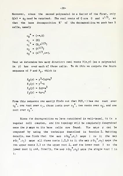
Moreover, since the second polynomial is a factor of the first, only

Q(x) " ^Q need be retained. The real roots of Q are and ^ ', so

that the base decomposition K' of the decomposition we seek has 5

cells, namely

-0

ci = {0}

1/3-

C2* = (a1/^+«).

Next we determine how many dinstinct real roots P(x,y) (as a polynomial

in y) has over each of these cells. To do this we compute the Sturm

sequence of P and Py, which is

fo(y> " y^-3xy+x3

fi(y) = y^-x

fjCy) = 2xy-x3

foCy) = 4x-x^

From this sequence one easily finds out that P(X, • ) has one root over

Cq , one root over Ci, three roots over Cj^ , two roots over C2, and one

root over Co .

Since the decomposition we have considered is well-based, it is a

regular cell complex, and its topology will be completely determined

once the p maps on its base cells are found. The maps p can be

computed by using the technique described in Section 2. Omitting

details, one finds that the map P (cq >Ci) maps 1 to 1; the map

pfcj^ ,0^) maps all three roots 1,2,3 to 1; the map p (cj ,C2) maps the

two upper roots 2,3 to the upper root 2, and the lower root 1 to the

lower root 1; and, finally, the map p (c2 ,Co) maps the single root 1 to

-39-

Appendlx B. On Exact Symbolic Computations with Algebraic Numbers.

This appendix addresses the problem f how to perform the exact

calculations with algebraic numbers required for the algorithms

described In this paper, fow which nvnnerlcal approximate solutions are

not acceptable, since such calculations may lead to Incorrect

conclusions, e.g. In comparing approximate quantities we may wind up

putting them In an order which is different from the order of the

original numbers, if these numbers are very close to each other. Of

course, the algorithms to be described will never be able to give an

'exact' value of an algebraic number. Nevertheless they can be used

whenever an answer to some discrete query involving algebraic numbers

is needed, as in the Collins decomposition related technique sketched

in this paper.

This kind of problem, i.e. how to perform exact calculations

involving algebraic numbers, has been studied by many authors (see

[Ak] , [He], [CL], [Ru]). In this appendix we will review the methods

used to perform calculations of this kind, describe various

improvements of techniques that have appeared in the literature, and

present a few additional techniques.

In the following discussion, we ignore all those (possibly

substantial) computational costs which can (and will) arise from the

growth in size of the Integers with which the algorithms to be

described must deal; that is, we will measure cost by assigning each

operation on Integers (and hence each elementary operation on rational

numbers) a nominal cost of 1. (Note however that much prior research

has concentrated on obtaining more realistic cost estimates for such

algorithms, taking into account the possible growth of coefficients

during certain operations on polynomials, such as computation of the

GCD of two polynomials, the Sturm sequence of a polynomial, the

sequence of derivatives of a polynomial, etc. (see [Br], [He], [CL]).

These more refined estimates have shown that the extra cost incurred in

such operations is still polynomial in the degree and the size of the

-40-

coefficients of the polynomial (s) involved. Our significantly more

optimistic cost measure is like the one used by Aho, Hopcroft and

Ullman [AHU].)

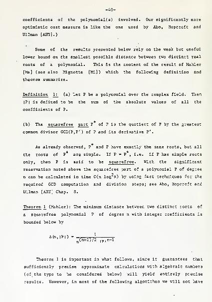
Some of the results presented below rely on the weak but useful

lower bound on the smallest possible distance between two distinct real

roots of a polynomial. This is the content of the result of Mahler

[Ma] (see also Mignotte [Mi]) which the following definition and

theorem summarize.

Definition 1

;

(a) Let P be a polynomial over the complex field. Then

IP Iis defined to be the sum of the absolute values of all the

coefficients of P.

(b) The squarefree part P of P is the quotient of P by the greatest

common divisor GCD(P,P') of P and its derivative P'.

As already observed, P and P have exactly the same roots, but all

the roots of P are simple. If P = P , i.e. if P has simple roots

only, then P is said to be squarefree . With the significant

reservation noted above the squarefree part of a polynomial P of degree

n can be calculated in time 0(n log n) by using fast techniques for the

required GCD computation and division steps; see Aho, Hopcroft and

Ullman [AHU] Chap. 8.

Theorem 1 (Mahler): The minimum distance between two distinct roots of

a squarefree polynomial P of degree n with integer coefficients is

bounded below by

A(n,|P|)^

jj(n+2)/2 ,p,n-l

Theorem 1 is important in what follows, since it guarantees that

sufficiently precise approximate calculations with algebraic numbers

(of the type to be considered below) will yield entirely precise

results. However, in most of the following algorithms we will not have

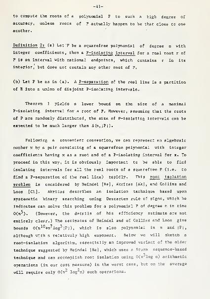
-Al-

to compute the roots of a polynomial P to such a high degree of

accuracy, unless roots of P actually happen to be that close to one

another.

Definition 2: (a) Let P be a squarefree polynomial of degree n with

integer coefficients, then a P-isolating Interval for a real root r of

P is an interval with rational endpoints, which contains r in its

interior, but does not contain any other root of P.

(b) Let P be as in (a). A P-separation of the real line is a partition

of R into a union of disjoint P-isolating intervals.

Theorem 1 yields a lower bound on the size of a maximal

P-isolating interval for a root of P. However, assuming that the roots

of P are randomly distributed, the size of P-isolating intervals can be

expected to be much larger than A(n,IP|).

Following a convenient convention, we can represent an algebraic

number x by a pair consisting of a squarefree polynomial with integer

coefficients having x as a root and of a P-isolating interval for x. To

proceed in this way, it is obviously important to be able to find

isolating intervals for all the real roots of a squarefree P (i.e. to

find a P-separation of the real line) rapidly. This root isolation

problem is considered by Heindel [He], Akritas [Ak] , and Collins and

Loos [CL]. Akritas describes an isolation technique based upon

systematic binary searching using Descartes rule of signs, which he

indicates can solve this problem for a polynomial P of degree n in time

O(n^). (However, the details of his efficiency estimate are not

entirely clear.) The estimates of Heindel and of Collins and Loos give

bounds O(n^^+n^log^ |P| ), which is also polynomial in n and |Pi,

although with 3 relatively high exponent. Below we will sketch a

root-isolation algorithm, essentially an improved variant of the older

technique suggested by Heindel [He], which uses a Sturm sequence-based

technique and can accomplish root isolation using 0(n log n) arithmetic

operations (in our cost measure) in the worst case, but on the average

will require only 0(n^ log^n) such operations.

-42-

We begin by reviewing the beautiful classical theory of Sturm

sequences (see Harden [Mar], p. 130 ff.), which gives a very useful way

of handling several of the problems that concern us. Let P be a

univariate polynomial, and let P' be its derivative. The Sturm

sequence of P is a sequence {f^^} of polynomials such that fg = P, fj

P', and such that for each i > 1, -f^^ is the remainder obtained by

dividing ^±-2 ^V ^i-l* ^°^ this sequence there plainly exists a

sequence of quotient polynomials Q^-i such that

h-2 "Qi-l^i-l -h' i > 1.

where the degree of f^ is strictly smaller than that of f^-i* Since P

is assumed to be squarefree, this process must terminate with some

constant function fi^. The Sturm sequence has the property that, for

any interval (a,b] the number of roots of P in this interval is S(a) -

S(b), where S(x) is the number of sign changes in the sequence [fgCx),

fl(x),..., fj,(x)].

Next we describe a fast procedure for the computation of the Sturm

sequence of a given polynomial P of degree n. At a first glance it

might seem that this task will require time at least O(n^), since that

many coefficients appear in the polynomials constituting this sequence.

However, by representing the sequence in a more economical way, we can

reduce this time to 0(n log^n) . To do this, we note that the degree of

Q^ is the difference of the degrees of f^-i and f^^ . Thus if m^^ denotes

the degree of the quotient Q^ , i=l,...,k-l, the sum of all the m^'s is

n. Hence we can represent the Sturm sequence by the sequence [fQ(x),

f^Cx), QjCx),..., Q^j_i(x)], which involves, only 0{n) coefficients.

Once this representation is available, we can use it to evaluate the

whole Sturm sequence at any given x, as well as the number of sign

changes m the Sturm sequence, in time 0(n). To do this, we first

compute fgCx), f^Cx), and Q^(x) for i=l,...,k-l (which requires total

time 0(n)). Then, using the 'backward formulae'

fi(x) = Qi(x)fi_i(x) - fi_2(x), i = 2,...,k,

-43-

the Stunn functions can be evaluated at x in 0(n) additional time.

For this more efficient evaluation, we simply need all the

quotient poljmomials Q^. Up to a sign change, these are exactly the

quotients obtained during calculation of the GCD of P and P'. To

compute all these quotients efficiently, we can use the fast pol3momial

GCD procedure described in [AHU], Chap. 8. This procedure works as

follows. Let a(x), b(x) be two polynomials of degree < n. Let the

remainder sequence {r^(x)} and the quotient sequence {q^(x)} of a(x)

and b(x) be defined so that rQCx) = a(x), r^Cx) = b(x), r^.^Cx) =

qi(x)ri(x) + ti+iCx"), i>l, and degCr^+^Cx)) < degCr^Cx)). For -each i

there exists a polynomial 2x2 matrix M. such that

(r^Cx), ri+i(x)] = [a(x), b(x)] M^.

Furthermore, each M^ is the product of matrices of the form

-qj(x) 1

1

N. =J < i.

The fast GCD algorithm first computes the two middle elements r .(x) and

r^^.i(x) in the remainder sequence, and then calls itself recursively

with rj(x) and r.^i(x) to process their remainder sequence, which of

course coincides with the rest of the remainder sequence of a and b. To

find r- and r-^.i, the algorithm uses another recursive procedure HGCD

which computes the matrix M-. This second procedure uses the fact (see

[AHU], Lemmas 8.6 and 8.7) that all the quotients q^Cx), i<j depend

only on the most significant half of the polynomials a and b. HGCD thus

discards the least significant halves of a and b, thereby obtaining

polynomials a' and b' of degree at most n/2; it then calls itself

recursively to compute the two middle elements r./ and r-z^j^ among the

first j elements in the remainder sequence of a' and b' , during which

process it also calculates the matrix M^*. The quotient qj'(x) and the

matrix N^/ are then calculated, after which HGCD calls itself once more

with r^' and t^a'+i as parameters to compute the product L of the

-44-

aatrices N . /^^ , . . . ,Nj. The matrix Mj is then computed as Mj'»Nj'«L,

and recursively returned. This description should make it plain that

the algorithm sketched computes all quotients q^(.x) appearing in the

quotient sequence of a(x) and b(x) . With minor modifications, it can

therefore be used to obtain the desired efficient representation of the

Sturm sequence of a given poljTiomial. Since the fast GCD algorithm

runs in time 0(n log n) , this is also the time required for the

calculation of the Sturm sequence.

This gives us the following

Theorem 2; The number of distinct real zeroes of a polynomial with

rational coefficients of degree n, lying in any given interval [a,b]

can be found in 0(n) arithmetic operations, after preprocessing which

requires 0(n log n) arithmetic operations.

We can now describe a root-isolation procedure as follows. We

first compute the Sturm sequence of the given polynomial P, in the

manner just described. Next we find an upper bound b and a lower bound

a such that all real roots of P lie in the interval [a,b]. For example

(see [Mar]), we can take

Pib « -a = max { 1+— : i = 0,...,n-l }

Pn

where p^ is the coefficient of the i-th power of x in P. Let N = S(b) -

S(a) denote the number of distinct real roots of P. We perform a binary

search of the interval I = [a,b] to find a point c e [a,b] which

separates it into two subintervals each containing at least one root of

P. It follows from Mahler's theorem that such a point will be found

after at most 0(n logn) bisecLxotib of i, at each of which we have to

evaluate S, so that to find c will take 0(n logn) steps. (However,

assuming random distribution of the roots of P, the expected number of

required bisections will be O(logn) , so that c will be found on the

average after 0(n log-n) steps.) We then apply the same process to each

of the intervals [a,c] and [b,c], and continue in this manner until

-A5-

isolating intervals for all the roots of P have been found. Obviously

only N < n intervals will have to be processed, so that the whole

procedure requires 0(n^ logn) steps in the worst case, and 0(n^ log^n)

steps on the average; note that these time bounds also dominate the

time required for the initial computation of the Sturm sequence.

An alternative, and possibly more attractive, technique for root

isolation has been described by Collins and Loos [CL], and is based on

Newton's approximation technique. Their technique proceeds inductively

by first obtaining root-separating intervals for the derivative of P,

making sure that none of these intervals contains a root of the second

derivative of P. On any interval in the complement of the union of

these intervals P' has constant sign, so that it is trivial to check

whether such an interval contains a root of P. On any of the

P'-isolating intervals I, P is either convex or concave throughout I.

Hence Newton's technique will converge (very rapidly) to a root of P in

I if such a root exists. This enables one to partition I rapidly into

P-isolating intervals which do not contain a zero of P' , thus allowing

iteration of the process. More details can be found in [CL].

Once any root isolation procedure is available, we can use it to

perform various exact computations in algebraic numbers. Before

describing efficient procedures for such computations, we first note a

simple but useful generalization of Sturm's theorem. Specifically, let

A(x) and B(x) be two given polynomials, where A is squarefree. Form

the generalized Sturm sequence of A and B (which, up to sign changes,

coincides with the remainder sequence of A and B) as follows. Put

i-1 (x) = qi(x)fi(x) - fi+i(x)

so that the last element in this sequence will be the GCD of A and B.

Let S(x) denote the number of sign changes in the sequence

[fnCx) , ... ,fi.(x)] . As in the case of fc ndard Sturm sequences, it is

easy to see that each time we cross a zero of some function f^(x), i >

1, S(x) remains unchanged. However, each time we cross a zero xq of fg

-46-

» A from left to right, S(x) decreases by sign(A'(xQ)B(xo)). (It is

easy to check that this statement remains true even if xq is a zero of

B(x).) Hence, in any given interval [a,b],

S(a) - S(b) = I sign(A'(x)B(x)),

where the svmmation extends over all distinct roots of A lying in

(a,b). (In the case of a standard Sturm sequence, B(x) = A'(x), so

that the above sum is equal to the number of distinct real roots of A

in (a,b).)

In particular, if the interval (a,b) is known to contain just one

root r of A(x), then S(a) - S(b) is 0,i or -1, depending on the signs

of A'(r) and B(r). Since A has been assumed to be squarefree, the sign

of A'(r) is easily calculable from the signs of A(a) and A(b). Hence

the sign of B(r) can also be calculated. That is, given an algebraic

number r, represented as the i-th root of a squarefree polynomial A,

for which an A-separation of the real line is available, and another

polynomial B, we can find the sign of B(r). (Note that (an efficient

representation of) the generalized Sturm sequence can be computed and

evaluated using precisely the same techniques prescribed for standard

Sturm sequences.) This technique improves that described by Rump [Ru]

.

This generalized Sturm technique is applicable to a variety of

other problems. For example, we can use it to determine the

multiplicity of the real roots of a given polynomial P. To do this, we

first compute the squarefree part P of P, and then isolate the real

roots of P* (i.e. the distinct real roots of P). For each root r of

P, we use the above procedure to determine sign P'(r). If this is

nonzero, then r is a simple root. Otherwise r has multiplicity 2 at

least; we then repeat our procedure to find the sign of P''(r), and so

on, until a nonzero sign is obtained, from which the multiplicity of r

is immediately calculable. Using this technique, the multiplicities of

2all real roots of a polynomial of degree n can be found in time 0(n

log n) (assuming that a P-separation is available). Indeed, the total

-Ay-

number of roots is n, and to determine each multiplicity, an 0(n log n)

procedure is applied.

A very similar procedure can be used to compare two real algebraic

numbers a and b, given as roots of the squarefree polynomials P and Q

respectively. To do this, obtain a P-separation and a Q-separation of

the real axis, and merge them into one partitioning. Let I = [c,d] be

a P-isolating interval for a, and let J = [e,f] be a Q-isolating

interval for b. If I and J are disjoint, then the manner in which a and

b compare is immediately obvious. Suppose then that I and J intersect.

Several cases can arise; we_will treat only the case in which c < e < d

< f , since the other cases can be handled in a similar manner. Since P

is squarefree, and since (c,d) contains only one root of P, P(c) and

P(d) have different signs. By evaluating the sign of P(e) we can

determine whether a lies in the subinterval (c,e) or in the subinterval

(e,d) of I. If a lies in (c,e) then we must have a < b. Similarly, if b

lies in (d,f) we also have a < b. In the remaining case, both a and b

(but no other root of P or Q) must ]'3 in the interval (e,d). Using

the generalized Sturm technique xplained above, we can compute the

sign of P(b), and this shows at once how a and b compare. As before,

this procedure takes 0(n log n) time, where n is the maximal degree of

P and Q, provided that P- and Q-separations of the real axis are

available.

Similar procedures can be used to perform various other exact

computations with algebraic numbers. Suppose, for example, that we

need to compare the sum (or product) of two algebraic numbers a and b

to a third such number. One can of course compute a polynomial R(x)

having a+b (or ab) as a root. However, it may be undesirable to do

this since this can generate a polynomial whose degree is deg(A) • deg(B)

(where A(x) (resp. B(x)) is a polynomial having a (resp. b) as a

root), and repeated computations of this sort may result in polynomials

of extremely large degrees. To avoid this problem, a recursive

symbolic representation of algebraic numbers might be more

advantageous: We can specify an algebraic number r either as a

polynomial A(ri , . . . ,rj^) in k other algebraic numbers, or as a root of a

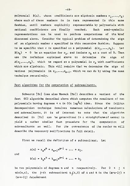
-48-

polynomial B(x), whose coefficients are algebraic numbers r,,...,ri.;

where each of these numbers is in turn represented in this same

fashion, until nvmbers explicitly representable by polynomials with

rational coefficients are finally reached. Such semi-symbolic

representations can be used to perform computations of the kind

discussed above. Consider the typical problem of determining the sign

of an algebraic number r specified in this recursive fashion. Suppose

to be specific that r is specified as a polynomial ACr^ , . . . ,r^^) . Let

B(rj^) = be an equation for t^, and isolate r^^ as a root of B. Then

use the technique explained above to determine the sign of

ACrj, .. .,rj^) , which we regard as a polynomial in t-^ with coefficients

which are algebraic. This will require that we determine the sign of

various polynomials in r^^ , . . . ,r^_2 » which we can do by using the same

technique recursively.

Fast algorithms for the computation of subresultants.

Schwartz [Sc] (see also Moenck [Mo]) describes a variant of the

fast GCD algorithm described above which computes the resultant of two

polynomials having degrees < n in 0(n log n) time. Since the Collins

decomposition technique involves numerous calculations of resultants

and subresultants, it is of interest to note that the algorithm

described in [Sc] can be generalized in a straightforward manner to

yield a rather similar fast procedure for the computation of

subresultants as well. For the convenience of the reader we will

describe the necessary modifications in full detail.

First we recall the definition of a subresultant. Let

A(x) = a„x™ + a„_,x™~^ + ...^m-1

,jX -r ... -r aQ,

and

B(x) = b^x"+ Vl^""^ + ... +bo

be two polynomials of degrees m and n respectively. For < j <

min(m,n), the j-th

(m+n-2j) determinant

min(m,n), the j-th subresultant i|».(A,B) of A and B is the (m+n-2j) >;

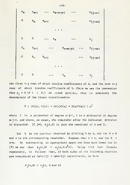
sl-1

-49-

^n-nrl-j+1

'n-1

^2j-n+l

^2j-n+2

^2j-iiH-l

^2j-m+2

the first n-j rows of which involve coefficients of A, and the last m-j

rows of which involve coefficients of B. (Here we use the convention

that Ej if i 0.) As noted earlier, this is precisely the

determinant of the linear transformation

T : [U(x), V(x)] * (A(x)U(x) + B(x)V(x)) / x^

where U is a polynomial of degree n- j-1 , V is a polynomial of degree

m-j-1, and where, as usual, the remainder after the indicated division

is discarded. If j=0, 4//A,B) is just the resultant of A and B.

Let Q be the quotient obtained by dividing B by A, and let R = B

mod A be the corresponding remainder. Suppose that n > m, and let k <

n-m. By subtracting an appropriate upper row from each lower row in

(*) we see that il-jCA.B) = i<) •(A,B-x'^A) . Using this last formula

repeatedly, it follows that, if both sides of the following equation

are considered as (m+n-2j) x (m4-n-2j) determinants, we have

i^j(A,B) = 'i'jCA, B mod A)

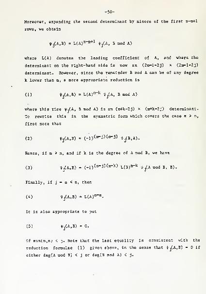
-50-

Moreover, expanding the second determinant by minors of the first n-m+1

rows, we obtain

i|»j(A,B) » L(A)°"^^ i|»j(A, B mod A)

where L(A) denotes the leading coefficient of A, and where the

determinant on the right-hand side is now an (2m-l-2j) x (2m-l-2j)

determinant. However, since the remainder B mod A can be of any degree

k lower than m, a more appropriate reduction is

(1) i|'j(A,B) = L(A)"~^ ipj(A, B mod A)

where this time tj(A, B mod A) is an (mfk-2j) x (nrl-k-2j) determinant.

To rewrite this in the symmetric form which covers the case m > n,

first note that

(2) i|'j(A,B) = (-l)(°-J)(^-J) if;j(B,A).

Hence, if m > n, and if k is the degree of A mod B, we have

(3) i|'j(A,B) = (-i)(n-j)(in-k) L(B)°^^ ^'/Amod B, B).

Finally, if j = m < n, then

(A) *j(A,B) = LCA)"-"".

It is also appropriate to put

(5) *j(A,B) = 0.

if min(.m,n; < j. Note that the last equality is consistent with the

reduction formulae (1) given above, in the sense that ;|;j(A,B) = if

either deg(A mod B) < j or deg(B mod A) < j.

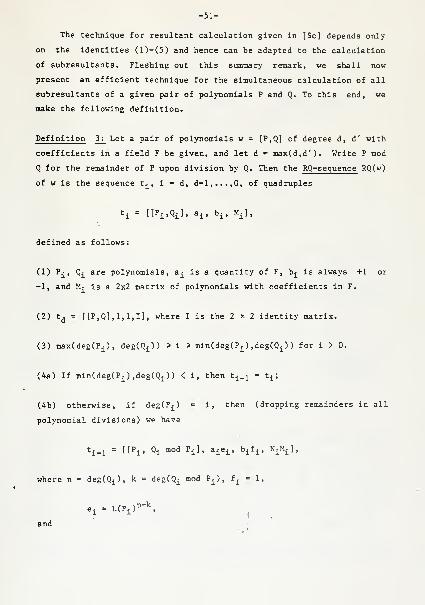
-51-

The technique for resultant calculation given in [Sc] depends only

on the identities (l)-(5) and hence can be adapted to the calculation

of subresultants. Fleshing out this summary remark, we shall now

present an efficient technique for the simultaneous calculation of all

subresultants of a given pair of polynomials P and Q. To this end, we

make the following definition.

Definition 2l ^^^ a pair of polynomials w = [P,Q] of degree d, d' with

coefficients in a field F be given, and let d = max(d,d'). Write P mod

Q for the remainder of P upon division by Q. Then the RQ-sequence RQ(w)

of w is the sequence tj, i = d, d-l,...,0, of quadruples

ti = [[Pi.Qi], a^, bi, M^],

defined as follows:

(1) P^, Q^ are polynomials, a^ is a quantity of F, b^^ is always +1 or

-1, and >L is a 2x2 matrix of polynomials with coefficients in F.

(2) tj =[ [P,Q],1, 1,1], where I is the 2 x 2 identity matrix.

(3) roax(deg(P^), deg(Q^)) > i > min(deg(P^) ,deg(Q^) ) for i > 0.

(4a) If min(deg(Pi),deg(Qi)) < i, then t^.^ = t^;

(4b) otherwise, if deg(P^) = i, then (dropping remainders in all

polynomial divisions) we have

^i-1 = ff^i' ^i ™°^ ^i^' ^i^i' ^i^i' ^i^^'

where n «= deg(Q^), k = deg(Q^ mod P^), f^^

= 1

,

e^ = L(Pi)"-^,

and

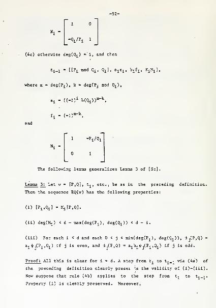
-52-

•Qi/Pi 1

(4c) otherwise deg(Qj^) ='i, and then

ti_i = ([Pi mod Q^, Q^], a^e^, b^f^, ^li^]

where m = degCP^), k » deg(Pj mod Q^),

e^ = ((-l)i L(Q.))'i =

f. - (-1)

\m-k

m-k

and

1 -Pi/Qi

1

The following lemma generalizes Lemma 3 of [Sc].

Lemma 3; Let w = [P,Q], t^, etc., be as in the preceding definition.

Then the sequence RQ(w) has the following properties:

(i) [Pi.Qil = MilP.Q].

(ii) deg(Mi) < d - max(deg(Pi), degCQ^)) < d - i.

(iii) For each i < d and each < j < min(deg(P^), degCQ^)), il'jCP.Q) =

a^tjCPi.Qi) if j is even, and ^/jCP.Q) = a^b^ij' jCP^ ,Qi) if j is odd.

Proof; All this is clear for i = d. A step from t^ to t^_j^ via (4a) of

the preceding definition clearly presei "s the validity of (i)-(iii).

Now suppose that rule (4b) applies to the step from t^ to ^±~i'

Property (i) is clearly preserved. Moreover,

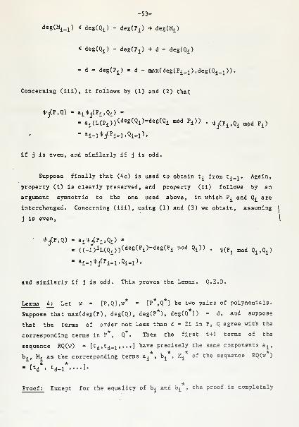
-53-

deg(M^_l) < deg(Qi) - degCP^) + deg(Mi)

< deg(Qj^) - deg(Pi) -)- d - degCQ^)

- d - degCP^) - d - inax(deg(Pi_i),deg(Qi_i)).

Concerning (iil), it follows by (1) and (2) that

i|»j(P,Q) = a^il-jCPi.Qi) -

- ai(L(Pi))('^^g(Qi>-deg(Qi mod Pi)) . 4,.(p^,Q^ ^^d Pi)

- ai-i*j(Pi-l.Qi-i),

if j is even, and similarly if j is odd.

Suppose finally that (4c) is used to obtain ti from t.^^-^. Again,

property (i) is clearly preserved, and property (ii) follows by an

argument symmetric to the one used above, in which Pi and Qi are

interchanged. Concerning (iii), using (1) and (3) we obtain, assuming

j is even,

• 4'j(P,Q) = aiT|<j(Pi,Qi) =

- ((-l)iL(Qi))(de8(Pi)-<^eg(Pi "o*^ Qi)> . H^^ mod Qi,Qi)

- ^i-l^j^Pi-l'Qi-l)'

and similarly if j is odd. This proves the Lemma. Q.E.D.

Lemma 4: Let w = [P,Q],w = [P ,Q ] be two pairs of polynomials.

Suppose that max(deg(P), deg(Q), deg(P*) , deg(Q*)) = d, and suppose

that the terms of order not less than d - 2i in P, Q agree with the

corresponding terms in P*, Q*. Then the first i+1 terms of the

sequence RQ(w) = [t^j.t^.j , . . . ] have precisely the same components ai,

bj, Mi as the corresponding terms ai*, bi*. Mi* of the sequence RQ(w )

Proof: Except for the equality of bi and bi , the proof is completely

-54-

identical to that of Lemma A of [Sc]. The equality of b^ and b^^ is

also an easy consequence of that same proof. Q.E.D.

Lemmas 3 and A justify the following subresultant calculation

algorithm, whose underlying idea is to compute the terms a^,b^ and Mj^

by stepping through the sequence [t^] by steps of increasing length,

each of length double that of the preceding step. Lemma 4 implies that

each of these steps can use polynomials of substantially lower degree

than that of the original polynomials. However, as soon as we have

calculated a^, b^ and M^ for some i < d for whic j = deg(P^) < deg(Q^),

we can get ^Ji?,Q) directly. Indeed, using (4) and Lemma 3(iii)-^ we

have

^p,q) ' aiii.^Pi,Qi)

= ai.UPi)('^^g(Qi)-j\

if j is even, and similarly if j is odd (and of course analogous

formulae are available if j = deg(Q^) < degCP^).) Note that if t^ * tj_/

then min(deg(Pj_),deg(Qi)) ^ min(deg(Pj_' ) ,deg(Q^' )) , so that for each j

either there exists no i for which j = mln(degCPj_ ,Q^) , or the i's for

which this eqiiality holds all have the same value t^, and hence the

above formula defines i|»^ unambiguously. Observe finally that, by (5),

all i{/ ^ which do not appear in the above formula for any value of i are

0.

In view of these comments, the algorithm proceeds as follows.

Initialize four static lists, AL, BL, CL and DL to the null list each.

(1) Call an auxiliary routine HSBRSL(P, Q, 0). This routine will build

up tne rirst half of the RQ-sequence [t^], for d > i > d/2 = d' , and

will return the quantities e^/ , f^^', and M^/

.

(2) Compute [Pd'.Qd'l "^^d' ^^d'^d^ •

(3) Let m = deg(P^j'), n » deg(Q^'). If m < n then append the

-55-

quantities e^/, f^/, L(PjjO"~". m respectively to the end of the four

lists AL, BL, CL, DL. Similarly, if m > n then append the quantities

e^j', fjj/, L(Qj')°~". n, to the end of these four respective lists.

(4) Call the whole procedure recursively, passing P^/, Q^/ to it as

inputs to complete the construction of the whole sequence.

The subprocedure HSBRSL(P,Q, £) required is rather similar to the

auxiliary procedure HGCD used in the fast polynomial GCD algorithm in

[AHU]. It consists of the following steps.

(1) Discard the least significant half of the coefficients of P and Q,

that is, let P = P*x^ + P', Q = Q*x^ + Q', where k =

max(deg(P),deg(Q))/2, and where deg(P'), deg(Q') < k.

(2) Apply HSBRSL to P , Q , and £-tk, to obtain e^> , fy_> and n^' for k'

= 3k/2 (by Lemma 4, these are the same as the corresponding quantities

associated with the original P and Q.)

(3) Compute [Pk'.Qk'l = ^k' f^'Q^'

(4) As in step (3) of the main procedure, let m = deg(Pj^')-, n =

deg(Q^'). If m < n then append the qviantities e^', f j^' , L(Pjj^')"~™.

m+£, to the end of the four lists AL, BL, CL, DL respectively.

Similarly, if m > n then append the quantities e^' , f^' , L(Qj^/)°~",

n+Z, to the end of these four respective lists.

(5) Let Pj^/ = P\'X^" + P", Q^^' = q\'X^" + Q", where k" = k/2,

and where deg(P"), deg(Q") < k".

(6) Call HSBRSL with p\' , q\' and i-^" , to obtain 6*^^, f*^ and M*j^.

(7) Return e j^, f j^, and M k*^'*

When the algorithm just sketched has terminated, we can perform one

-56-

final scan through the lists AL, BL, CL, and DL, to accumulate the

scalar quantities a^^ and bj^ by repeated multiplication of the e^'s and

the f^'s respectively. Using the following technique we can also

calculate all the subresultants \|; j. For each iteration step k, let y-^,

nijj be the k-th components of CL and DL respectively, and let ai^-j and

b^_j be the product of all preceding components in the lists AL and BL

respectively. If m^ is even, put

*i^ = ^k-l^k.

and if mj^ is odd, put —

*n^ = ai,_ibk.iYk-

At the end of this final iteration, all remaining undefined

subresultants are set to 0.

The computational cost of the procedure just sketched is evidently the

same as the original procedure given in [Sc]. To estimate this cost we

note that multiplication and division of polynomials of order m can be

accomplished in time 0(m log m) . During each call to the subprocedure

HSBRSL(P,Q, £ ) that we have just described polynomials of order at most

m=max(deg(P),deg(Q)) need to be multiplied and divided (at steps (3)

and (7)). The total time T(m) required to apply HSBRSL to two

polynomials of degree m therefore satisfies T(2m) = 2T(m) + 0(m log m)

and hence has the bound T(m) = 0(m log m) . Similar considerations show

that the time used by the main procedure to build up the RQ-sequence

has the same bound, so that this estimate also bounds the time required

to calculate all the subresultants of two polynomials of maximal degree

-57-

Appendix C. Adjacency of Collins Cells of General Dimension.

In this appendix we complete our calculation of Collins cell

adjacency by considering cells whose dimension is less than that of the

whole space E'^ being decomposed. The problem here is to determine when

a Collins cell c' of dimension k-1 is a face of a cell c of dimension k

< r. Our approach will again be based upon consideration of the base

decomposition K' of K. However, the present case is somewhat more

complex than the case k = r considered previously, and this makes it

necessary to use a bit more (largely classical) machinery drawn from

the theory of algebraic curves. Accordingly, we recall the following

definitions and lemmas, for which see Keller [Ke], Chap. 5.

Definition 1

;

(a) A fractional (Laurent) series is a formal series of

the form

(1) y(x) = I a^xi=m

i/D

whose coefficients are complex numbers, and in which D is an integer.

Such a series is said to be convergent if it converges in the

neighborhood of x = 0. Note that we allow m to be negative. The series

(1) is said to be truncated if it contains only finitely many terms.

(b) If a^^ t 0, then m/D is called the leading exponent of the series y.

(c) If the leading exponent e of the series (1) satisfies e > k (resp.

e > k), we will write y = O(x^) (resp. y = o(x^)).

It is easily seen that the standard definitions of addition,

multiplication, etc. for power series make the collection of all

fractional series into a field. This statement, like many others made

in the next few paragraphs, is true irrespective of whether we consider

convergent fractional series only, or allow arbitrary, nonconvergent

series, and treat operations on them in a purely formal manner.

-58-

Moreover, this statement remains true even if the coefficients of the

series (1) are required to lie in some subfield of the complex numbers.

In what follows we will designate the field of fractional power

series by Fr.

Lemma 1; (see [Ke] , Chap. V) The field of fractional series with

complex (or with algebraic) coefficients is algebraically closed.

Thus if P(y) = a^^y" + ... + aQ is a polynomial in y with

coefficients in the field Fr_and if a^^ * 0, P can be factored as

(2) P(y) ="ap(y-ri) ... (y-r„)

,

where rj^,...,rjj are themselves fractional series, namely the roots of

P(y) =0.

In what follows we will need to work in purely finite manner with

fractional series representing the roots of various polynomials. Our

ability to do so without ambiguity will rest upon various extensions of

the following simple lemmas, which are also noted by Kung and Traub

[KT].

Lemma 2: Let P(x,y) be a polynomial with complex coefficients in two

variables, of total degree d>0. Let its degree n in y be nonzero, and

aj^(x) which is not zero for x=0. Regard P^Cy) as a polynomial in y

with coefficients in Fr, and let r^ (x) , . . . ,r^(x) be its roots (which

are elements of Fr) . Then

(a) If z^U) - rj(x) = 0(x^(2n-l))^ ^.^gn i = j.

(b) We cannot have ?^' (r^ix)) = o(x'^^^^~^h for any root r^(x).

Proof; Consider the discriminant D(x) of the polynomial Px(y)> i«e« ^

-59-

^^^^^x'^x'^ ^^ ^^^ resultant of P^^ and P^'. This is a polynomial of

degree d(2n-l) in x, and since P^^ and P^^' have no factor in common it

is nonzero. Hence D(x) = o(x^^^"~^^) is impossible. By well-knovm

identities (see [Wa], Sections 30 and 31),

(3) D(x) = n (ri(x)-rj(x))

and also

(A) D(x) = n Pj^'Cr^Cx)).

is easy to see (by substitution) that no fractional series r(x) with

negative leading exponent can satisfy P^(r(x)) = 0. Hence r^(x) = 0(1)

for all i, and therefore if assertion (a) of our Lemma were violated,

(3) would imply that D(x) = o{x'^^^^~^^) , which is impossible. If we

use (4) instead of (3) in this argument, (b) follows in the same way.

Q.E.D.

Lemma 3: Let P^(y) = aj,(x)y" + a^_^(x)y""^ + ... + ao(x) be a

polynomial in y, of degree n, with coefficients in Fr, and suppose that

a (x) does not vanish at x = 0. Let k > 1, and let Vq = "[a^x ' be an

element of Fr such that Pj^(yQ(x)) = 0(x"^). Then there exists a root

r^(x) of PjjCy) = such that yQ(x)-ri(x) = O(x^).

Proof; Factor Px(y) in the manner (2). Then it is plain that if Vq-t^i

has leading exponent less than k for all i, the leading exponent of

P (yg(x)) must be less than nk, contradicting our assumption. Q.E.D.

Lemma 3 asserts that any power series yg which comes close enough

to making ^x^^O^ equal to zero must lie quite close to a root of P^^.

It is also worth noting that if Pv^y) ^^ "° repeated roots, then, once

P (yg) has been made small enough, any desired number of coefficients

of a root of Pjj(y)=0 can be calculated rapidly from the coefficients of

Yq by purely rational operations. A technique for calculating

fractional power series which approximate each of the roots of ^^^(y)

-60-

near x=0 to an arbitrary degree of precision is described by Kung and

Traub [KT]. Their technique uses first the Newton's polygon method to

obtain an initial (truncated) fractional series approximation for each

of the roots of P^^, and then uses a variant of Newton iteration

(similar to that described by Lipson [Li]) to extend each of these

series to an arbitraru degree of precision. Kung and Traub give a

complexity bound of 0(nN log N) for their procedure, where n is the

y-degree of the polynomial P^^, and where N is the number of terms

sought in each fractional series. This bound holds' asymptotically if n

is held fixed and N increases, but it ignores the cost of applying the

Newton polygon procedure (which indeed is independent of N) in order to

obtain the initial number of terms required to ensure convergence of

Newton's approximation method. At present our best estimates of this

cost are still exponential, leading us to pose the following

Open Problem: Given a polynomial P(x,y) with complex coefficients, of

y-degree n and total degree d, does there exist a procedure for

calculating truncated fractional series approximations for each of the

roots of P(x,y) (regarded as a polynomial in y) near x=0 up to terms of

order 0(x'^^^^~^^) , in time polynomial in n and d?

As will become clear from the subsequent discussion, an

affirmative answer to this problem would imply that adjacency of

Collins cells of general dimension, and hence also the homology groups

of any algebraic variety, can be calculated in time polynomial in the

number and the maximal degree of polynomials defining a Collins

decomposition (or an algebraic variety).

At any rate, once these fractional power series are available, we

can use them to determine the adjacency of Collins cells. It is worth

explaining what is involved by commenLxng Drieiiy on the special case r

- 3. Let K' be the 2-dimensional base decomposition of a well-based

Collins decomposition K of E"^ whose base polynomial is P(x,y,z). Let c

be a 1-dimensional curved cell in K', and let c' = [xQ,yQ] £ K be an

endpoint of c. Let Q(x,y) be the base polynomial of K' . It follows

from the preceding discussion that in the vicinity of c' the curve c

-61-

can be specified uniquely by a truncated fractional series y(x) which

approximates the corresponding root of Q(x,y) near (xQ.yg). If enough

leading terms of this fractional series are known, then, to determine

the number of roots of P(x,y,») into which a given root Zq of

P(xQ,yQ,z) = splits as we move from (xQ,yQ) into c, we can substitute

the curve y(x) for y in P, thus obtaining a polynomial R^Cz) "

P(x,y(x),z) in z with coefficients in Fr. Then, using a Sturm-based

technique of the sort described in Appendix B, we can determine the

number of roots of R^ into which zq splits for sufficiently small

positive x. We can also compute truncated fractional series

approximating each of these roots, and this enables us to carry the

same form of analysis inductively to cases involving more than three

variables.

However, several technical difficulties must be overcome in

following this conceptual approach. First of all, Lemma 2 is not

immediately applicable to R^, since the coefficients of R^ are not

simply polynomial but lie in Fr; moreover R^ need not be squarefree.

This makes it a little harder to state how many terms of a fractional

series suffice to characterize a root of ^v^^) uniquely. Also, the

truncated fractional series y(x) gives only an approximate

representation of the root of Q which traverses the curve c, and at

first glance it is not clear how many terms need be included in y(x) to

guarantee that the analysis we have outlined will carry forward

inductively.

To overcome these purely technical difficulties, it is useful to

consider systems of polynomial equations in several variables having

the form specified in the following definition.

Definition 2; (a) A triangular monic system of polynomial equations is

a system

P2(xi,X2) =

(5) P3(xi,X2,X3) =

-62-

P„(xi,X2,...,x„) -

of polynomial equations of total degrees d2,...,djj with complex

coefficients, whose j-th eqxiation involves the variables Xj^ , . . . ,xj

only, and which, regarded as a polynomial in x^ with coefficients

polynomial in the remaining variables, has a constant leading term.

The sequence d2,...,dj^ is the degree sequence of the triangular system

(5).

(b) Given the triangular monic system (5), its resultant system is the

sequence

(6) R2(xi,X2), R3(xi,X3), .... R^Cx^.Xj^)

of bivariate polynomials defined as follows. R2 is simply ?2' ^3 ^^

obtained from P3 and P2 by regarding them both as polynomials in the

variable X2 and forming their resultant. More generally, to form

R^(x^,x^) proceed as follows: Regard Pj(x^,..,Xj) and Pj_i (x^ , . . ,Xj_j)

as polynomials in x- j, and form their resultant, thus obtaining a

polynomial QjCx^ , . . ,Xj_2,Xj) from which the variable Xj_^ has been

eliminated. Then form the resultant Q2 of Q^ and Pj_2 (as polynomials

in ^i-2^» obtaining a polynomial from which both variables x- 2 and

x^_2 have been eliminated. Continue repeatedly in this way, thus

finally obtaining the desired polynomial R- = Q^_2» from which all

variables but Xj^ and x^ will have been eliminated.

(c) The sequence 62, . . ., 6^ of degrees of the resultant polynomials (6)

is called the resultant degree sequence of the triangular system (5).

Definition 3: (a) A solution curve of the triangular monic system (5)

is a continuous vector-valued function f(t) = [f 2(t) , . . .,f^( t) ] with

complex components defined for all sufficiently small nonnegative

values of the parameter t, such that for all j=2,...,n we have

Pj(t,f2(t),...,fj(t)) = 0.

(b) Let P^ and f be as in (a), let d = [d2,...,djj] be a sequence of

-63-

rational numbers, and let a= [02,..., aJ be a sequence of truncated

fractional series in the variable t, such that a^ contains terms of

order 0(t j) at most. Then a is said to be an order d^ descriptor of

the solution curve f if fj-Oj " 0(t*^j) for all j'=2,...,n.

Our aim is to generalize Lemmas 2 and 3 to general triangular

monic systems of more than two variables. For this, we need the

following straightforward technical lemma, whose main purpose is to

enable us to bound the order of finite descriptors of solution curves

of (5) needed to characterize such a solution uniquely.

Lemma 4; As in Definition 3, let P2,...,Pji be a triangular monic system

and let R2,...,Rn be its resultant sequence. Then each R. can be

factored as

(7) Rj(xi,Xj) = A(xi)r5(xi,Xj)rJ(xi,Xj),

where A, R^ and R^ are all polynomials in their respective variables,

and where R^ is the squarefree part of R^ (regarded as a polynomial in

xp represented by a polynomial whose coefficients (which are

polynomials in Xi) have no common factor. Moreover, we can arrange

,0this factorization so that the leading coefficient C(x^) of Rj does not

vanish at Xi = 0.

Proof; As in Definition 2, regard P -(xj^ , . . . ,Xj) and Pj_i (x^ , . . . ,x •^

)

as polynomials in x^.^ with polynomial coefficients, and form their

resultant Q^. If we use the fact that P^.j is monic in x- 2, it

follows from the fundamental theorem of resultant theory that a tuple

[xj, .. . ,Xj_2,Xj] is a solution of the system Pj = P2 = ... = Pj_2 = Qi

= of equations if and only if there exists an x.j^such that

[xj, .. . ,Xj_2,Xj_j,Xj] is a solution of the system P^ = 0, i=2,...,j.

Arguing repeatedly in this way, we see that [xj,x^] is a solution of

the equation R.(xi,Xj) = if and onl- if there exist X2,...,Xj_j such

that [x2,X2 xJ is a zero of .^ for all i=2,..,j. On the other

hand, it follows since each P^ is monic that all the solutions of the

system P^ = 0, i=2,..,j which lie over a small neighborhood of the

-64-

point X, remain bounded. Thus all the solutions of Rj(x2^,Xj)=0

over such a neighborhood have the same property.

Next regard Rj as a polynomial in Xj, take its (x^-) derivative

Rj, form T^ « GCD(Rj,RS), and use it to factor Rj.as Rj = T°T^. These

are polynomials in x^ with coefficients rational in xj , but then by

multiplying through by an appropriate polynomial CCxj^) we can write CR^

« S^S , where now S^ and S^ have coefficients which are polynomials in

xj. Since the ring of polynomials in two variables is a unique

factorization domain, every prime factor of C divides one of the

polynomials on the right, which is to say, divides all its

coefficients. This remark allows us to divide through by all these

prime factors, and if we then collect all common factors of the

coefficients of R and R^ in A(xi^), we arrive at the factorization (7).

It is now clear' that all the solutions [x^.Xj] of Rj=0 which lie

over a sufficiently small neighborhood of Xj=0 have second components

Xj which remain bounded. By Lemma 1, these solutions r^ (xj) , . . . ,r^(xi

)

can be written as fractional power series V a^xj ', so that since they

remain bounded near X2=0 none of these fractional series contain any

term with negative exponents. Suppose that the leading coefficient

ajjj(xj) of Rj vanishes at x^=0. Then since R^ can be factored as

R^Cxj.Xj) = aj^Cxj) n(xj-rj_(xi)),

it would follow that all the coefficients of R^ vanish at Xj^=0. But

then Xj would be a common factor of all coefficients of R^, contrary to

the way in which R^ has been defined. Q.E.D.

Corollary; Let the polynomials P^, j=2,..,n form a triangular monic

system, and let the resultant degree sequence of this triangular system

be (62...-. 5J- Put

d = [62(262-1), ..., 6^(26^-1)].

Then any two solution curves f(t), g(t) of this triangular system which

-65-

have identical order d descriptors are identically equal for all

sufficiently small nonnegative values of t.

Proof; Let Rj be the resultant system of the triangular system P^.

Arguing as in the proof of Lemma 4, we can conclude that the components

f J of f satisfy R^(x,f^(x)) = 6, and similarly for the components of g.

Our assertion is therefore an immediate consequence of Lemmas 2 and 4.

Q.E.D.

Definition 4: Let P^ and 5^ be as in the preceding Corollary, let d =

[d2,...,djj] be the degree sequence of the P^, and define d =

* Amax dodo • 'd^e. (26^-1). Put d^ = d /(d2»'i) for j=2,..,n, (so thatj=2^ .n J J J J J

d^ is a decreasing sequence of positive rational numbers). Suppose

that for j=2,..,n a Ax) is a truncated fractional series such that

there exist auxiliary truncated fractional series a.(x) (all of whose

exponents can be assumed to be < d^) such that P^(x, a2(x) , . . . ,a .(x) ) =

0(x<^j-l) and aj(x) - aj(x) = O(x'^j). Then a = [02, '...aj is called an

adequate descriptor for a_ solution of the triangular system P2 = . . . =

Lemma 5; Let d, d , and 6 be as in the preceding definition. Given any

adequate descriptor a = [02, ...,a^] for a solution of the triangular

system (5), then for all sufficiently small t there exists a solution

f(t) = [f2(t),..,fn(t)] of the system Pj(t,f 2(t) , . . . ,f ^(t) ) = 0,

j=2, .. ,n such that

(8) f j(t) - a.(t) = Oit^P^f^h.

Proof; Use the notations of Definition 4. We proceed by induction on j

to establish the existence of a solution curve f = [f2,..,f^] which

satisfies the formula

(8') fj(t) - aj(t) - O(t'^j),

for j « 2,..,n. By definition of the d- it is plain that (8') implies

(8). The base case j=2 for our induction is immediate from Lemma 3.

-66-

Suppose that we have already shown the existence of f2(t) , . . . ,fj.^Ct)

such that Pj^(t,f2(t),...,fi(t)) = for i=2,..,j-l, and such that (8')

holds for all such i. As in definition 4, there exist auxiliary

fractional series a^(t) such^that Pj(t .OjCt) , . . . ,a j(t) ) = OCt'^j-l) and

a*(t) - a^(t) - 0(t*^i) < O(t^j-l) (since the d* are decreasing). Thus

by (8') we have a^(t) - fj_(t) = 0(t j-1), from which we see immediately

that

Pj(t,f2(t),...,fj.i(t),a*(t)) = O(t'^j-l).

Hence by Lemma 3 there exists a root f^(t) of this same equation such

that fj(t) - aj(t) - 0(t^^2-^^^2h = O(t^j) for small t, from which

(8') is plainly seen to hold for j too. Q.E.D.

Corollary; Let Pj, f = [f 2, • • .f^l > and a = [02, . . ,aJ be as in Lemma 5.

Suppose that all the polynomials P^ have real coefficients. Then f^ is

real if and only if all the nonzero coefficients appearing in a- ^re

real.

Proof ; Since all P^ are real, the whole situation being considered is

invariant under complex conjugation. Thus the curve I - [l2i««>?n^ ^^

also a solution curve of the system P-, and a = [02,.., a^] is an

adequate descriptor for J. It is plain from Definition 3 and from the

corollary to Lemma 4 that f = f if and only if a = a, from which the

present corollary is immediate. Q.E.D.

Our preparation is now sufficient for computations of the

topological relationships which interest us to be feasible. The

following definition takes the next step in this direction.

Definition 5; Let K be a Loiiins aecomposltion of the Euclidean space

E'^, let c be a d-dimensional cell in K, and let c' e K be a

(d-l)-dimensional face of c. Then an incidence curve for the pair ci, c'

is a triple consisting of

-67-

,P_ of m polynomials with real

algebraic coefficients,

(ii) a continuous solution curve f(t) = [f ^Ct) ,f 2(t) , . . . ,fj.(t) ] all of

whose components are real such that f(t) e c for all sufficiently small

nonnegative t, and such that f(0) e c'. All constant components of the

vector f must be algebraic numbers, and its nonconstant components

f^ (t),...,f£ (t), which for convenience we shall write in1 m

left-to-right order as gj (t) , . . . ,g^(t) , must satisfy P^Cg^ (t) , . . ,gj(t)

)

" for j=2,..,m. Moreover, gjCt) must have the form g^Ct) = t+5 ,

where C is an algebraic number.

(iii) An adequate descriptor a for the solution g2,...,gj, of the

triangular monic system P2 = . . • = Pjj^ = 0. This (finite) descriptor

will be used to represent the nonconstant components of the curve f in

finite terms in a unique manner.

Our aim is to carry such a family of incidence curves through the

whole inductive construction of the Collins decomposition, and at each

stage to use them to determine which (d-1 )-dinensional cells c' are

faces of a given d-dimensional cell c. To this end, let K be a

well-based decomposition of E^, and let K' be the base decomposition of

K. Suppose inductively that for each cell b of K' and each of its faces

b' of one less dimension an incidence curve for the pair b, b' is

available. Let c be a d-dimensional cell of K, and let c' be one of

its faces. Then, by Lemma 3 of Section 2, either c = b^ for some b e

K' and c' = b. or c' =^i+i> or c = b^ and c' = bj' where b' is a

(d-2)-dimensional face of (the (d-1 )-dimensional) cell b, or c = b- and

c' = bj' where b' is a (d-1 )-dimensional face of (the d-dimensional)

cell b.

Let P(xj, . . . ,Xj.) be the base polynomial of K; since K is

well-based, the leading coefficient of P (regarded as a polynomial in

Xj.) is constant. If c = b^ ano c' = b^, then we can take

[Zi ^1^1 ] to be any algebraic point in b, and then if Z j. is the

j-th root of P(;i, ..., ;j^l,Xj.) we can put f(t) = [^j, . . . ,? j^j , ? j.+t] ,

-68-

thereby defining an incidence curve. Of course, an entirely similar

construction yields an incidence curve for the pair c^, c^^j.

Next suppose that c - bj and c' - bj , where b' is a

(d-2)-dimensional face of b. Let f - [fjCt) ^r-l^^^^ ^^ ^°

incidence curve for the pair b, b' , let gj(t) = 5-rt:,g2(t) , . . . .g^j^Ct) be

the nonconstant components of this curve, enumerated in left-to-right

order, and let P2,..,Pjj be the associated triangular monic system of

polynomials. Put ;j=fj(0) for j«=l,..,r-l, so that the point Z =

[Cj, .••.Cr«l] is an algebraic point in b' . Let P be as in the

preceding paragraph, lit n be the J-th real root of P(C j, . . ,? j-.! ,y) •=

(or a sufficiently small rational nvimber if J=0), and let n' be the

(J+l)-st root of this same equation (or a sufficiently large rational

number if this equation has only J real roots). Put 5^. = _(Ti4n'), and

f(t) = [f i(t) ,.. . ,fj._2(t) , ^j.] . This is plainly an incidence curve for

the pair c, c' , whose nonconstant components are plainly the same as

those of f. We have an adequate descriptor for the nonconstant

components of f ' , and plainly" this can also serve as an adequate

descriptor for f.

Finally, suppose that c = b^ and c' = bj, where b' is a

(d-l)-dimensional face of b. Again, let f'(t) = [f ^(t) , . . ,f ^..^ (t) ] ,

[P2, . .. .Pj^^] , and a' - [ 02, . . . , a^^l ] be an incidence curve for the

pair b, b'. As in Definition 5, let gi,...,gnj_i be the nonconstant

components of f, so that g2(t) = t+Z where C is algebraic, and put

Oj(t) = t+C for convenience. Extend the truncated fractional series

aJ,

j=2,..,m-l to series a* such that gj - a* = 0(t°), where D will be

chosen below. Let P be the same base polynomial as in the two

preceding paragraphs, let d be its degree, and let P be the polynomial

obtained from P by replacing each variable x- in it for which f^(t) =

? :. is an algebraic constant by ;« Clearly, the degree of P" is at

most d. Having P*, we can then find all distinct real rootsyi,...,yjj_

of the equation P*( a^(0) , . . , o^^ (0) ,y) » and arrange these solutions

in increasing order. By Lemma 2 of Section 2, these roots are in 1-1

correspondence with the sequence of 'section' cells b^ of K whose base

cell is b'. Next, for each such yj^, we can find all the fractional

-69-

series solutions of the monic equation P (.a^it) ,. ,. ,a^^^(t.) ,y) =

whose constant term is y^^; all terms of these series up to those of

order t must be constructed. Let a(t) designate any one of the

truncated fractional series constructed in this way. Since g-^-Q-; =

O(t^) for j=l,..,m-l, we have P*(gi(t) , . . . ,g„_l(t) ,a(t)) = 0(t°) and

thus by Lemma 3 there exists a solution g of P (gj^Ct) , . . . ,gjjj_j(t) ,g(t) )

" such that a(t)-g(t) «= 0(t^'*^). Append the polynomial P* to the

triangular monic system P2, • • • fP^j-i » thus obtaining a larger system

P2,...,P^, and let R2,...,R,jj and 62, ....fij^ be respectively the

resultant system and the resultant degree sequence of this extended

system. Arguing as in the first paragraph of the proof of Lemma 4, we

see that R^i^Si (t) ,g(t) ) = R^it+Z ^(.t)) = 0. Hence if we choose D =

d6 (2 6 -1) it follows by Lemma 2 that this equation, together with the

truncated fractional series ,a and the relationship g-a = 0(t^'°),

determine g uniquely, and in particular (arguing as in the proof of the

Corollary to Lemma 5) that g is real for t>0 if and only if all the

coefficients of the fractional series a are real.

Dropping all those fractional series a which involve any nonreal

coefficient, we can then go on to append any of the remaining a to

aj, . . • »anj_l . thereby obtaining an adequate descriptor for the

nonconstant components of the curve f = [fj^, . . . .fj-.i ,g] , where g is the

unique (real) solution of R^(t+?,g(t)) represented by a. Let us agree

to compare any two fractional series B(t), T (t) with real coefficients

by comparing coefficients of like terms lexicographically; this is

equivalent to agreeing that 6 < y if 6(t) < Y(t) for all sufficiently

small nonnegative t. Then it is plain that for each y^ the real

solutions of P*(gi(t), ..,g^_i(t),g(t)) = are in 1-1 ordered

correspondence with the truncated fractional series a which we retain

and which satisfy a(0) = yj^. The number of such series is therefore

the number of distinct real roots into which the root y^ of

P(;i, ..,? i,y) = splits as f'(t) moves from the point f'(0) =

[?i, ..,C j] of b' to ir-^ediately neighboring points inside b. The

sequences Pj, . . . ,Pjn_i ,P' gi , • • .g,!,-! .g. ^^^ « 1> • • Om-l »** clearly define

incidence curves for all pairs of cells having the form bj, bj, such

that the latter is part of the boundary of the former.

-70-

This finishes our inductive construction of incidence curves, and

also shows how the information on root splitting needed to determine

the mappings pCb,b'), defined in the paragraph preceding Lemma 3 of

Section 2, can be calculated; so that description of a technique for

testing the adjacency of Collins cells of general dimension is now

complete.

Remark: Given two Collins cells and Tarski sentences defining each of

them, we can easily write a quantified Tarski sentence which is true if

and only if they are adjacent. Thus in principle we can obtain an

adjacency-testing algorithm using standard decision-procedures for

Tarski sentences. Howe-'er, since the number of quantified variables

required to define adjacency of Collins cells in this way can be large

(compare e.g. the explicit Tarski sentence defining a Collins cell

given at the end of Appendix A), this technique will probably be much

less efficient than that described in the present Appendix.

i

Acknowledgement (

The authors would like to thank Professor Dennis Arnon for his

generous help during the preparation of this paper.

Bibliography

1

[AHU] A. Aho, J. Hopcroft and J. Ullman [1974] The Design and

Analysis of Computer Algorithms. Addison-Wesley, Reading, Mass.

[Ak] A.G. Akritas [1980] The Fastest Exact Algorithm for the Isolation

of the Real Roots of a Polynor il Equation. Computing v. 2A,

pp. 299-313.

[Ar] D.S. Arnon. [1981] Algorithms for the Geometry of Semi-Algebraic

-71-

Sets. Tech. Rept. A36, Computer Science Department, Unlverity

of Wisconsin, Madison.

lAr2] D.S. Arnon [1982] Automatic Analysis of Real Algebraic Curves.

Tech. Rept., Computer Science Department, Purdue University.

[BT] W.S. Brown and J.F. Traub [1971], On Euclid's Algorithm and the

Theory of Subresultants. JACM v. 18, pp. 505-514.

[Ch] P.J. Cohen [1969] Decision Procedures for Real and p-adic Fields.

Comm. Pure and Appl. Math. v. 22, pp. 131-151

[Co] G. Collins [1975] Quantifier Elimination for Real Closed Fields by

Cylindrical Algebraic Decomposition, in: Second GI Conference

on Automata Theory and Formal Languages, Lecture Notes in

Computer Science v. 33, Springer Verlag, Berlin, pp. 134-183.

[CL] G.E. Collins and R. Loos [1976] Polynomial Real Root Isolation

by Differentiation, in: SYMSAC 76 (Proc. of the 1976 ACM

Symp. on Symbolic and Algebraic Computations, Yorktown

Heights, N.Y.) pp. 15-25.

[CF] G.E. Cooke and R.L. Finney [1967] Homology of Cell Complexes.

Mathematical Notes, Princeton University Press, Princeton,

New Jersey.

[Ha] W.R. Hamilton [1969] Elements of Quaternions, Chelsea Pub. Co.

New York.

[He] L.E. Heindel [1971] Integer Arithmetic Algorithms for Polynomial

Real Zero Determination. JACM v. 22, pp. 533-549.

[Hi] H. Hironaka [1975] Triangulations of Algebraic Sets, in: Proc.

Symposia in Pure Math. v. 29, A ican Math. Soc, Providence.

R.I., pp. 165-185.

-72-

[IKP] M.B. Ignat'yev, F.M. Kulakov and A.M. Pokrovskiy [1973] Robot

Manipulator Control Algorithms. Report No. JPRS 59717, NTIS

Springfield, Va.

[Ke] O.H. Keller [1974] Vorlesungen Uber Algebraische Geometrie.

Akademische Verlagsgesellschaf t , Geest & Portig, Leipzig.

[KT] H.T. Kung and J.F. Traub [1978] All Algebraic Functions can be

Computed Fast. JACM v. 25, pp. 245-260.

[La] D. Uzard [1977] Algebre Lineaire sur K[X^ X„] et

Elimination. Ball. Soc. Math. France, v. 105, pp. 165-190.

[Li] J. Lipson [1976] Newton's Method: A Great Algebraic Algorithm.

in: SYMSAC 76 (proc. ACM Symp. on Symbolic and Algebraic

Computations, Yorktown Heights, N.Y.), pp. 260-270.

[LPW] T. Lozano-Perez and M. Wesley [1979] An Algorithm for Planning

Collision-Free Paths Among Polyhedral Obstacles. CACM v. 22,

pp. 560-570.

[Ma] K. Mahler [1964] An Inequality for the Discriminant of a

Polynomial. Michigan Math. J. v. 11, pp. 257-262.

[Mar] M. Marden [1949] The Geometry of Zeroes of a Polynomial in a

Complex Variable. Mathematical Surveys v. 3, Amer. Math.

Soc, Providence, R.I.

[Mi] M. Mignotte [1976] Some Problems About Polynomials, in: SYMSAC

76 (Proc. 1976 ACM Sjnnp. on Symbolic and Algebraic Computations.

7oikwv.wii Heights, N.Y.), pp. 227-228.

[Mo] R. Moenck [1973] Studies in Fast Algebraic Algorithms. Ph.D.

Dissertation, University of Toronto.

[Re] J. Reif [1979] Complexity of the Mover's Problem and

-73-

Generalizations. Proc. 20th Symp. on the Foundations of

Computer Science, pp. A21-427.

[Ru] S. Rump [1976] On the Sign of a Real Algebraic Number, in:

SYMSAC 76 (Proc. 1976 ACM Symp. on Symbolic and Algebraic

Computations, Yorktown Heights, N.Y.), pp. 238-241.

[Sc] J.T. Schwartz [1980] Fast Probabilistic Algorithms for

Verification of Polynomial Identities, JACM v. 27, pp.

701-717.

[SS] J. SchvTartz and M. Sharir [1981] On the 'Piano-Movers' Problem; I.

The case of a Two-Dimensional- Rigid Polygonal Body Moving

Amidst Polygonal Barriers. Computer Science Technical Report

39, Courant Institute, New York University. To appear in

Comm. Pure and Appl. Math.

[Ta] A. Tarski [1951] A Decision Method for Elementary Algebra and

Geometry. (Second Edition, Rev.) University of California

Press.

[Ud] S. Udupa [1977] Collision Detection and Avoidance in Computer-

Controlled Manipulators, Ph.D. Dissertation, California Inst.

of Technology, Passadena, Ca.

[Wa] B.L. Van der Waerden [1939] Einfuhrung in die Algebraische

Geometrie, Springer Pub. Co., Berlin.

[Wa2] B.L. Van der Waerden [1960] Algebra (5th Edition) Springer

Pub. Co., Berlin.

This l>ook may be kept

FOURTEEN DAYSA fine will be charged for each day tbo book is kept overtime.

lUU ^

NYU ^ • ^

Comp. Sci. Dept.TR-41SchwartzOn the 'piano movers' problem,II,

NYUComp . Sci .Dept

.

Sohwartam;^On the 'piano movers'

problem. II.

DATE DUE BORROWER S

4^y^ \v^^ l>ofi$ i

N.Y.U. Courant Institute of

Mathematical Sciences

251 Mercer St.

New York, N. Y. 10012