Embed Size (px)
Citation preview
a
ces,
er-for theich
lternatest cel-
Advances in Applied Mathematics 34 (2005) 798–811
www.elsevier.com/locate/yaam
On the refined 3-enumerationof alternating sign matrices
F. Colomoa, A.G. Pronkob,∗
a INFN, Sezione di Firenze, and Dipartimento di Fisica, Università di Firenze,Via G. Sansone 1, 50019 Sesto Fiorentino (FI), Italy
b Sankt-Petersburg Department of V.A. Steklov Mathematical Institute of Russian Academy of ScienFontanka 27, 191023 Sankt-Petersburg, Russia
Received 6 May 2004; accepted 16 September 2004
Abstract
An explicit expression for the numbersA(n, r;3) describing the refined 3-enumeration of altnating sign matrices is given. The derivation is based on the recent results of Stroganovcorresponding generating function. As a result,A(n, r;3)’s are represented as 1-fold sums whcan also be written in terms of terminating4F3 series of argument 1/4. 2005 Elsevier Inc. All rights reserved.
1. Introduction
An alternating sign matrix (ASM) is a matrix of 1’s, 0’s and−1’s such that in each rowand in each column the first and the last nonzero entry is 1, and all nonzero entries ain sign. There are many nice results concerning ASMs (for a review, see [1]). The mo
* Corresponding author.
E-mail address:[email protected] (A.G. Pronko).0196-8858/$ – see front matter 2005 Elsevier Inc. All rights reserved.doi:10.1016/j.aam.2004.09.007
F. Colomo, A.G. Pronko / Advances in Applied Mathematics 34 (2005) 798–811 799
s,] that
finedt
s the
ted
s, i.e.,
ebrated result gives the total numberA(n) of n × n ASMs. It was conjectured by RobbinMills and Rumsey [2,3] and subsequently proved by Zeilberger [4] and Kuperberg [5
A(n) =n∏
k=1
(3k − 2)!(k − 1)!(2k − 1)!(2k − 2)! =
n∏k=1
(3k − 2)!(2n − k)! . (1.1)
Yet another formula was conjectured in [2,3], and proved in [6], concerning the reenumeration of ASMs, namely, that the number ofn×n ASMs with their sole 1 of the firs(or last) column (or row) at ther th entry, denoted asA(n, r), is
A(n, r) =(n+r−2n−1
)(2n−1−rn−1
)(3n−2
n−1
) A(n). (1.2)
One more conjecture of Robbins, Mills and Rumsey, proved by Kuperberg [5], givenumber of 3-enumerated ASMs. In general,x-enumeration counts ASMs with a weightxk ,wherek is the total number of−1’s in each matrix (the numberx here should not beconfused with the variablex below). The total number of 3-enumerated ASMs is denoasA(n;3) and the result reads
A(2m + 1;3) = 3m(m+1)
m∏k=1
[(3k − 1)!(m + k)!
]2
,
A(2m + 2;3) = 3m (3m + 2)!m![(2m + 1)!]2
A(2m + 1;3). (1.3)
In the present paper we study the problem of the refined 3-enumeration of ASMwe derive the numbersA(n, r;3). The main result can be summarized as follows.
Theorem (Main result). The refined3-enumeration of ASMs,A(n, r;3), is given by
A(2m + 2, r;3) = b(m, r − 1) + b(m, r − 2)
2A(2m + 2;3),
A(2m + 3, r;3) = 2b(m, r − 1) + 5b(m, r − 2) + 2b(m, r − 3)
9A(2m + 3;3), (1.4)
where the quantitiesb(m,α), obeyingb(m,α) = b(m,2m − α), are given by
b(m,α) = (2m + 1)!m!3m(3m + 2)!
[α/2]∑�=max(0,α−m)
(2m + 2− α + 2�)
(3m + 3
α − 2�
)
×(
2m + � − α + 1
m + 1
)(m + � + 1
m + 1
)2α−2� (1.5)
for α = 0,1, . . . ,2m, while they are assumed to be zero for all other values ofα.
800 F. Colomo, A.G. Pronko / Advances in Applied Mathematics 34 (2005) 798–811
oth’),ne
cturesedhis,sults inld sum
nctionwetion 3antlytion 4,
e
-
been
c--
As a comment to the main result it is to be mentioned that the numbersA(n, r;3) appearnot to be writable as a single hypergeometric term, i.e., not to be ‘round’ (or ‘smocontrarily to the expressions forA(n), A(n, r) andA(n;3). For instance, direct inspectioof the results of computer experiments forA(n, r;3) shows the appearance of large primfactors in their prime factorizations, strongly suggesting that no answer forA(n, r;3) canbe given in the form of a single hypergeometric term. This explains why no conjeconcerningA(n, r;3) was given previously, and it might moreover imply that any cloexpression forA(n, r;3) could be at best a sum of several ‘round’ terms. In view of tthe expression in formulae (1.4) and (1.5), even if not as elegant and neat as other rethe context of ASM enumerations, is probably the best that can be achieved: a 1-foof ‘round’ terms.
Our proof of the theorem is based on a certain representation for the generating fufor the numbersA(n, r;3), recently obtained by Stroganov [7]. In the next sectionrecall the relevant formulae of paper [7] and shortly review their backgrounds. In Secwe apply standard relations for Gauss hypergeometric function to simplify significStroganov’s expression for the generating function of 3-enumerated ASMs. In Secfrom this simplified expression we obtain explicit formulae forA(n, r;3), thus proving thetheorem.
2. Preliminaries
In studying the refined 3-enumeration ofn × n ASMs it is convenient to define thgenerating function
H(3)n (t) = 1
A(n;3)
n∑r=1
A(n, r;3)tr−1, H (3)n (1) = 1. (2.1)
A simple property of the generating function isH(3)n (t) = tn−1H
(3)n (t−1), which follows
from the relationA(n, r;3) = A(n,n − r + 1;3) expressing left–right (top–bottom) symmetry within the set ofn × n ASMs.
In paper [7] the following defining properties of the generating function haveestablished. The generating functionsH
(3)n (t) for n even,n = 2m + 2, and forn odd,
n = 2m + 3, are related by the formulae
H(3)2m+2(t) = (t + 1)
2B2m(t), H
(3)2m+3(t) = (2t + 1)(t + 2)
9B2m(t), (2.2)
where B2m(t) is some polynomial of degree 2m. It is convenient to defineEm(t) :=t−mB2m(t) so thatEm(t) = Em(t−1). The functionEm(t) can be related to another funtion Vm(x), obeying, in turn, the relationVm(x) = Vm(x−1), by means of the transformation
Vm(x) x − q
Em(t) =(x − 1+ x−1)m, t = −
qx − 1, (2.3)
F. Colomo, A.G. Pronko / Advances in Applied Mathematics 34 (2005) 798–811 801
e
s ob-the
. The] (see
] forctionalt the
ion
-ations
or, inversely,
Vm(x) = 3mEm(t)
(t + 1+ t−1)m, x = t + q
tq + 1, (2.4)
where (and everywhere below) the following shorthand notation is used
q := exp(iπ/3). (2.5)
The function
hm(x) := (x − x−1)2m+1(
x + 2+ x−1)Vm(x) (2.6)
is found to be
hm(x) = cm
(gm(x) + 3m + 2
3m + 1fm(x)
), (2.7)
where the functionsfm(x) andgm(x) are given by
gm(x) :=m∑
k=0
(m + 2/3
k
)(m − 2/3
m − k
)(x3m+2−6k − x−3m−2+6k
), (2.8)
fm(x) :=m∑
k=0
(m + 1/3
k
)(m − 1/3
m − k
)(x3m+1−6k − x−3m−1+6k
), (2.9)
andcm is some constant such thatVm(1) = Em(1) = 1. For the reader’s convenience wnote that the variablex here and the variableu of Ref. [7] are related by e2iu = −x−1.
The result just described for the generating function of 3-enumerated ASMs watained by analyzing Izergin’s determinant formula [8] for the partition function ofsix-vertex model with domain wall boundary conditions (also known as ‘square ice’)one-to-one correspondence of square ice states with ASMs was pointed out in [9also [10]) and fruitfully applied by Kuperberg in [5]. The approach proposed in [111-enumerated ASMs and extended to 3-enumerated ASMs in [7], uses a certain funequation for the square ice partition function. This functional equation is nothing buBaxter’s T-Q equation for the ground state of XXZ Heisenberg spin-1/2 chain at∆ = −1/2and with odd number of sitesN = 2m + 1, studied previously in [12].
In particular, expression (2.7) forhm(x) arises as the solution of the functional equat
y(x) + y(q2x
) + y(q−2x
) = 0 (2.10)
which is supplemented by the condition that its solutiony(x) = hm(x) must have thestructure (2.6) where the functionVm(x) is supposed to be such thatVm(eiϕ) is an eventrigonometric polynomial of degreem in the variableϕ. This condition allows one to reduce the functional equation to a finite set of linear algebraic equations. These equ
can be solved explicitly thus leading to the formula forhm(x).
802 F. Colomo, A.G. Pronko / Advances in Applied Mathematics 34 (2005) 798–811
ion
cen-at solu-
atuation.
ential
hyper-
tity
The functionsfm(x) andgm(x) are also solutions of Eq. (2.10), and by constructthey have the structure
fm(x) = (x − x−1)2m+1
Qm(x), gm(x) = (x − x−1)2m+1
Pm+1(x), (2.11)
whereQm(x) andPm+1(x) are such thatQm(eiϕ) andPm+1(eiϕ) are even trigonometripolynomials of degreesm andm + 1, respectively. These two functions are two indepdent solutions of T-Q equation. Note that as the second independent solution (i.e., thtion which is of higher degree) one can also regard the functionPm+1(x)+ 3m+2
3m+1Qm(x) aswell as any function of the formPm+1(x)+αQm(x), see [13]. Thus, (2.7) just implies th3-enumerated ASMs are described by the second independent solution of T-Q eqThe first solution,Qm(x), was shown in [11] to be related to 1-enumerated ASMs.
Namely, in the case of 1-enumerated ASMs it was shown that
H(1)n (t) = const× Qn−1(x)
(qx − q−1x−1)n−1, t = qx−1 − q−1x
qx − q−1x−1, (2.12)
where the generating functionH(1)n (t) is defined similarly to (2.1) by
H(1)n (t) := 1
A(n)
n∑r=1
A(n, r)tr−1, H (1)n (1) = 1. (2.13)
To reproduce formulae (1.1) and (1.2) from (2.12) it was proposed to use the differequation satisfied byfm(x), which reads
[∂2ϕ − 6mcot3ϕ∂ϕ − (3m + 1)(3m − 1)
]fm
(eiϕ) = 0. (2.14)
Fortunately, the corresponding equation on the generating function appears to be ageometric equation
[(t − 1)t∂2
t + 2(t + n − 1)∂t − n(n − 1)]H(1)
n (t) = 0 (2.15)
and its polynomial solution gives
H(1)n (t) = (2n − 1)!(2n − 2)!
(3n − 2)!(n − 1)! 2F1
(−n + 1, n
−2n + 2
∣∣∣∣t)
. (2.16)
Here the proper normalization, see (2.13), follows from the Chu–Vandermonde iden
2F1
(−m,b
c
∣∣∣∣1)
= (c − b)m
(c)m, (a)m := a(a + 1) · · · (a + m − 1). (2.17)
SinceA(n,1) = A(n − 1), Eq. (2.16) results in an elementary recursion
A(n − 1) (1) (2n − 1)!(2n − 2)!
A(n)= Hn (0) =(3n − 2)!(n − 1)! (2.18)
F. Colomo, A.G. Pronko / Advances in Applied Mathematics 34 (2005) 798–811 803
g
ASMs.
func-h the
ltion
cane9)
to ae the
lts onh haveithinequa-
nd will
l-
which, supplemented by the initial conditionA(1) = 1, gives formula (1.1). ExpandinRHS of (2.16) in power series int and multiplying these coefficients byA(n), one repro-duces, in turn, formula (1.2).
Unfortunately, a similar procedure cannot be applied in the case of 3-enumeratedIt can be verified directly that the functionhm(x) solves the equation
{∂2ϕ − 3
[(2m + 1)cot3ϕ − 1
sin 3ϕ
]∂ϕ − (3m + 1)(3m + 2)
}hm
(eiϕ) = 0. (2.19)
This equation leads to a rather bulky nonhypergeometric equation for the generatingtion H
(3)n (t), which can hardly be solved by standard means. Moreover, even thoug
functionQm(x) can easily be deduced from the equation forfm(x) above, the differentiaequation forgm(x) (for this equation, see [12]) does not allow one to find the funcPm+1(x) in a similar way. As a matter of fact, only an implicit answer forH
(3)n (t) in terms
of two recurrences, generated by three-terms recurrences forfm(x) andgm(x), was givenin paper [7]. Here we would like just to mention that from differential equation (2.19) iteasily be seen that the operator(sin 3ϕ)−1∂ϕ plays the role of a ‘lowering’ operator in thset of trigonometric polynomials{hm(eiϕ)}. It is thus straightforward to rewrite Eq. (2.1as a three term recurrence forhm(x) and, hence, to obtain a single recurrence forH
(3)n (t).
However this point of view will not be developed further, since it amounts merelyreformulation of the problem. Instead, in the next section we show how to overcomdifficulty and find the functionH(3)
n (t) explicitly.As a last comment here we would like to mention that, although the previous resu
the refined 3-enumeration of ASMs run over papers [7,11,12], the present researcoriginated from our study of the square ice boundary correlators obtained in [14]. Wour study the refined enumerations of ASMs arise as solutions of some differentialtions rather than functional ones, in particular, the expression forhm(x) arises as a solutioof (2.19). The illustration of this approach is out of the scope of the present paper anbe given elsewhere [15]; here we restrict ourselves to obtaining the numbersA(n, r;3)
from the knownhm(x).
3. The generating function
We begin with noticing that the functionsfm(x) andgm(x) can be also written as folows
gm(x) = �(m + 1/3)
m!�(1/3)
[x3m+2
2F1
(−m,−m − 2/3
1/3
∣∣∣∣x−6)
− x−3m−22F1
(−m,−m − 2/3
1/3
∣∣∣∣x6)]
, (3.1)
fm(x) = �(m + 4/3)
m!�(4/3)
[x−3m+1
2F1
(−m,−m + 1/3
4/3
∣∣∣∣x6)
3m−1(−m,−m + 1/3
∣∣∣ −6)]
− x 2F14/3 ∣x . (3.2)
804 F. Colomo, A.G. Pronko / Advances in Applied Mathematics 34 (2005) 798–811
iffer byonscan be
n-f
auss
Since the parameters of the hypergeometric functions entering these expressions dintegers one can expect thatgm(x) andfm(x) are connected by some three-term relativia Gauss relations (see, e.g., Section 2.8 of [16]). Indeed, using Gauss relations itshown that
2F1
(−m,−m − 2/3
1/3
∣∣∣∣z)
= 3m + 4
22F1
(−m − 1,−m − 2/3
4/3
∣∣∣∣z)
− 3m + 2
2(1+ z)2F1
(−m,−m + 1/3
4/3
∣∣∣∣z)
(3.3)
and therefore we have the following relation
gm(x) = 3m + 2
2(3m + 1)
(x3 + x−3)fm(x) − 3(m + 1)
2(3m + 1)fm+1(x). (3.4)
Substituting (3.4) into (2.7) we obtain
hm(x) = cm
3m + 2
2(3m + 1)
[(x3 + 2+ x−3)fm(x) − 3m + 3
3m + 2fm+1(x)
]. (3.5)
Comparing Eqs. (3.4) and (3.5) with Eqs. (2.6) and (2.11) we find that
Pm+1(x) = 3m + 2
2(3m + 1)
(x3 + x−3)Qm(x) − 3(m + 1)
2(3m + 1)
(x − x−1)2
Qm+1(x) (3.6)
and
Vm(x) = cm
3m + 2
2(3m + 1)
[(x − 1+ x−1)2
Qm(x)
− 3m + 3
3m + 2
(x − 2+ x−1)Qm+1(x)
]. (3.7)
Hence all functions in question are expressed in terms ofQm(x)’s.The advantage of this approach is based on the fact that for the functionQm(x) the
following explicit formula can be found
Qm(x) = (2m)!3m(m!)2
(qx−1 − q−1x
q − q−1
)m
2F1
(−m,m + 1
−2m
∣∣∣∣qx − q−1x−1
qx−1 − q−1x
). (3.8)
As already mentioned in our preliminary comments, the functionQm(x) can be de-duced from the differential equation forfm(x) above (the proper normalization, for istance, can be found using the three-term relation forfm(x)’s). Here we give a prooof (3.8) by a straightforward transformation of the functionfm(x) to the formfm(x) =(x − x−1)2m+1Qm(x).
The key identity which is to be used here is the so-called cubic transformation of G
hypergeometric function [16] which in its most symmetric form reads:
F. Colomo, A.G. Pronko / Advances in Applied Mathematics 34 (2005) 798–811 805
r.3.2) in
ameter
�(a)
�(2/3)2F1
(a + 1/3, a
2/3
∣∣∣∣z3)
− ω−1z�(a + 2/3)
�(4/3)2F1
(a + 1/3, a + 2/3
4/3
∣∣∣∣z3)
= 3−3a+1(
1− z
1− ω
)−3a�(3a)
�(2a + 2/3)2F1
(a + 1/3,3a
2a + 2/3
∣∣∣∣ωz − ω
1− z
). (3.9)
Hereω is a primitive cubic root of unity,ω = exp(±2iπ/3), anda is arbitrary parameteTo show that indeed the cubic transformation is relevant to our case, let us rewrite (the form consistent with LHS of (3.9). Taking into account that
2F1
(−m,−m + 1/3
4/3
∣∣∣∣z)
= �(1/3)�(4/3)
�(−m + 1/3)�(m + 4/3)(−z)m2F1
(−m,−m − 1/3
2/3
∣∣∣∣z−1)
(3.10)
and
�(1/3)
�(m + 4/3)= (−1)m+1�(−m − 1/3)
�(2/3),
�(m + 4/3)
�(−m + 1/3)= (−1)m
(3m + 1)!33m+1 m! (3.11)
it is easy to see that (3.2) can be rewritten in the form
fm(x) = (−1)m+1(3m + 1)!33m+1(m!)2
x3m+1[�(−m − 1/3)
�(2/3)2F1
(−m,−m − 1/3
2/3
∣∣∣∣x−6)
+ x−2�(−m + 1/3)
�(4/3)2F1
(−m,−m + 1/3
4/3
∣∣∣∣x−6)]
. (3.12)
Clearly, both terms in the brackets are the same as in LHS of (3.9) provided the para is specialized to the valuea = −m − 1/3.
To apply the cubic transformation to (3.12) we first define
W(a; z) := �(a)
�(2/3)2F1
(a + 1/3, a
2/3
∣∣∣∣z3)
+ z�(a + 2/3)
�(4/3)2F1
(a + 1/3, a + 2/3
4/3
∣∣∣∣z3)
(3.13)
so that
(−1)m+1(3m + 1)! 3m+1 ( −2)
fm(x) =33m+1(m!)2x W −m − 1/3;x . (3.14)
806 F. Colomo, A.G. Pronko / Advances in Applied Mathematics 34 (2005) 798–811
tion,
ation[16]).
Next, we note that for a sum of two terms one can always write
X + Y = q
q − q−1
(X − q−2Y
) − q−1
q − q−1
(X − q2Y
)(3.15)
and ifq = exp(iπ/3), which is exactly the case, one can setω = q2 for the first pair of termsandω = q−2 for the second one. This recipe allows one to apply the cubic transformathat gives
W(a; z) = 3−3a+1�(3a)
�(2a + 2/3)
(1− z)−3a
q(1− q2)−3a+1
[2F1
(a + 1/3,3a
2a + 2/3
∣∣∣∣q2z − q2
1− z
)
+ q3a+12F1
(a + 1/3,3a
2a + 2/3
∣∣∣∣q−2z − q−2
1− z
)]. (3.16)
To obtain a new formula forfm(x) via (3.14) we have to evaluate now the limita →−m − 1/3 of (3.16). The limit of the pre-factor can be easily found due to
lima→−m−1/3
�(3a)
�(2a + 2/3)= 2
3
(−1)m+1(2m)!(3m + 1)! . (3.17)
To find the limit of the expression in the brackets in (3.16) we note that
q2z − q2
1− z=: s, q−2z − q−2
1− z= 1− s (3.18)
and hence the following formula can be used
lima→−m−1/3
[2F1
(a + 1/3,3a
2a + 2/3
∣∣∣∣s)
+ q3a+12F1
(a + 1/3,3a
2a + 2/3
∣∣∣∣1− s
)]
= 3
22F1
(−m,−3m − 1
−2m
∣∣∣∣s)
. (3.19)
Formula (3.19) can be proved, for instance, by virtue of standard analytic continuformulae for the hypergeometric function (see, e.g., Eqs. (1) and (2) in §2.10 ofCollecting formulae we arrive to the expression
W(−m − 1/3; z) = −32m+1(2m)!(3m + 1)!
(1− z)3m+1
(q − q−1)m2F1
(−m,−3m − 1
−2m
∣∣∣∣q2z − q2
1− z
). (3.20)
Finally, substituting this expression into (3.14) and using the identity
2F1
(a, b
∣∣∣∣z)
= (1− z)−a2F1
(a, c − b
∣∣∣∣ z)
(3.21)
c c z − 1
F. Colomo, A.G. Pronko / Advances in Applied Mathematics 34 (2005) 798–811 807
mationu-
isnde
we obtain
fm(x) = (2m)!3m(m!)2
(x − x−1)2m+1
(qx−1 − q−1x
q − q−1
)m
2F1
(−m,m + 1
−2m
∣∣∣∣qx − q−1x−1
qx−1 − q−1x
).
(3.22)
Obviously, this expression leads directly to (3.8) which is thus proved.Hence, we have just shown that a particular solution of Eq. (2.10), the functionfm(x),
Eq. (2.9), is connected to the ‘first’ solution of the Baxter T-Q equation,Qm(x), Eq. (3.8),via the cubic transformation. Formulae (3.4) and (3.5) mean that the same transforis responsible for relationship ofgm(x) and hm(x) with the second independent soltion of T-Q equation, which can be chosen either asPm+1(x), in the case ofgm(x), orasPm+1(x) + 3m+2
3m+1Qm(x) = (x + 2+ x−1)Vm(x), in the case ofhm(x).To write down the resulting expressions for functionsPm+1(x) andVm(x), and for the
purpose of subsequent transformation of these expressions, we define
Φ(k)m (x) :=
(qx−1 − q−1x
q − q−1
)m
2F1
(−m,k + 1
−m − k
∣∣∣∣qx − q−1x−1
qx−1 − q−1x
). (3.23)
Note that for positive integerm, function Φ(k)m (x) possesses the propertyΦ(k)
m (x) =Φ
(k)m (x−1) and thus, obviously,Φ(k)
m (x) is a polynomial of degreem in the variableu := x + x−1.
In particular, Eq. (3.8) now reads
Qm(x) = (2m)!3m(m!)2
Φ(m)m (x). (3.24)
Formulae (3.6) and (3.7) give
Pm+1(x) = 3m + 2
2(3m + 1)
(2m)!3m(m!)2
[(x3 + x−3)Φ(m)
m (x)
− 2(2m + 1)
3m + 2
(x − x−1)2
Φ(m+1)m+1 (x)
], (3.25)
Vm(x) = (2m)!(2m + 1)!m!(3m + 1)!
[(x − 1+ x−1)2
Φ(m)m (x)
− 2(2m + 1)
3m + 2
(x − 2+ x−1)Φ(m+1)
m+1 (x)
]. (3.26)
Here the expression forVm(x) is written according to the proper normalization of thfunction, Vm(1) = 1. The normalization can be verified by virtue of Chu–Vandermoidentity (2.17) and it corresponds to the choice
3m+1m!(2m + 2)!
cm = (3m + 1)(3m + 3)! . (3.27)
808 F. Colomo, A.G. Pronko / Advances in Applied Mathematics 34 (2005) 798–811
-lations
ns con-tions
intion
d
Formulae (3.25) and (3.26) for functionsPm+1(x) andVm(x) are not the final expressions for them yet since they can be notably simplified. Indeed, again using Gauss reone can prove, for instance, the following relations for the functions (3.23)
Φ(k)m+1(x) = (
x + x−1)Φ(k)m (x) − m(m + 2k + 1)
3(m + k + 1)(m + k)
(x2 + 1+ x−2)Φ(k)
m−1(x), (3.28)
Φ(k+1)m (x) = m + 2k + 2
2(m + k + 1)Φ(k)
m (x) + m
2(m + k + 1)
(x + x−1)Φ(k+1)
m−1 (x). (3.29)
These two relations can be regarded as basic relations; many other tree-term relationectingΦ
(k)m (x)’s can be derived from (3.28) and (3.29). Using these three-term rela
we find that for the functionPm+1(x), in particular, the following formula is valid
Pm+1(x) = (2m)!3mm!(m + 1)!
[(3m + 2)Φ
(m−1)m+1 (x) − (2m + 1)Φ
(m)m+1(x)
]. (3.30)
Similarly, for the functionVm(x) we obtain
Vm(x) = (2m)!(2m + 2)!(m + 1)!(3m + 2)!
[(2m + 1)Φ(m+1)
m (x) − m(x − 1+ x−1)Φ(m+1)
m−1 (x)]. (3.31)
This formula forVm(x) can be further simplified, due to (3.29), to be written solelyterms ofΦm(k)’s, but (3.31) is more convenient for the purpose of obtaining the funcEm(t), which is of primary interest for 3-enumerated ASMs. Applying (2.4) we obtain
Em(t) = (2m)!(2m + 2)!3m(m + 1)!(3m + 2)!
[(2m + 1)(t + 2)m2F1
(−m,m + 2
−2m − 1
∣∣∣∣ 1+ 2t
t (t + 2)
)
− 3m(t + 2)m−12F1
(−m + 1,m + 2
−2m
∣∣∣∣ 1+ 2t
t (t + 2)
)]. (3.32)
Formulae (3.30), (3.31) and, especially, (3.32) are the main results of this section.
4. The numbers A(n, r;3)
Let us begin with showing how Eq. (1.3) forA(n;3) is recovered from the just obtaineexpression for the generating function. Here the propertyA(n,1;3) = A(n − 1;3) is to beused. It implies
A(2m + 1;3)
A(2m + 2;3)= H
(3)2m+2(0) = 1
2B2m(0),
A(2m + 2;3) = H(3)
(0) = 2B2m(0). (4.1)
A(2m + 3;3) 2m+3 9
F. Colomo, A.G. Pronko / Advances in Applied Mathematics 34 (2005) 798–811 809
.u-
.t to the
ecomes
ofld likeay be
Hence, one has the recurrences
A(2m + 3;3) = 9[B2m(0)
]2A(2m + 1;3), A(1;3) = 1, (4.2)
A(2m + 2;3) = 9
B2m(0)B2m−2(0)A(2m;3), A(2;3) = 2. (4.3)
Recall thatB2m(t) = tmEm(t) in (2.2). From (3.32) one finds
B2m(0) = (2m + 1)!(2m + 2)!3m(m + 1)!(3m + 2)! . (4.4)
Substituting (4.4) into (4.2) and (4.3), and solving the recurrences one obtains (1.3)Let us now turn to our main target,A(n, r;3), which describes the refined 3-en
meration of ASMs. Formulae (2.2) imply that
A(2m + 2, r;3) = b(m, r − 1) + b(m, r − 2)
2A(2m + 2;3),
A(2m + 3, r;3) = 2b(m, r − 1) + 5b(m, r − 2) + 2b(m, r − 3)
9A(2m + 3;3), (4.5)
whereb(m,α) are defined as
B2m(t) = tmEm(t) =:2m∑α=0
b(m,α)tα (4.6)
and are assumed to be zero ifα is out of the range of values 0,1, . . . ,2m. To find thesecoefficients we expand (3.32) in power series int , thus expressingB2m(t) as a triple sumChu–Vandermonde summation formula can now be applied to the sum with respecindex defining the hypergeometric series in (3.32), thus expressingB2m(t) as a doublesum. These two summations can be rearranged in such a way that one of them bwith respect toα while the other one defines the coefficients of power expansion int . Weobtain
b(m,α) = (2m + 1)!m!3m(3m + 2)!
[α/2]∑�=max(0,α−m)
(2m + 2− α + 2�)
(3m + 3
α − 2�
)
×(
2m + � − α + 1
m + 1
)(m + � + 1
m + 1
)2α−2�. (4.7)
Here [α/2] denotes integer part ofα/2. Formulae (4.5) and (4.7) complete the proofthe theorem, which constitutes the main result of the present paper. Here we wouto mention that in terms of terminating hypergeometric series the last formula m
rewritten, for instance, as follows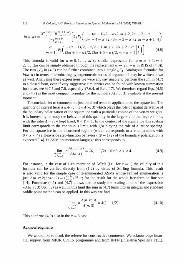
810 F. Colomo, A.G. Pronko / Advances in Applied Mathematics 34 (2005) 798–811
rdownn (4.7)ation
s. (4.5)t
e. Theofights.
ingg.
s
ulttion iseessionard
finan-
b(m,α) = 2α(3m+3
α
)(2m+1−αm+1
)3m
(3m+2m+1
)[24F3
( −(α − 1)/2,−α/2,m + 2,2m + 2− α
(3m + 4− α)/2, (3m + 5− α)/2,m − α + 1
∣∣∣∣1
4
)
− α
m + 14F3
( −(α − 1)/2,−α/2+ 1,m + 2,2m + 2− α
(3m + 4− α)/2, (3m + 5− α)/2,m − α + 1
∣∣∣∣1
4
)]. (4.8)
This formula is valid forα = 0,1, . . . ,m (a similar expression forα = m + 1,m +2, . . . ,2m can be simply obtained through the replacementα → 2m − α in RHS of (4.8)).The two4F3 in (4.8) can be further combined into a single5F4. Analogous formulae fob(m,α) in terms of terminating hypergeometric series of argument 4 may be writtenas well. Analyzing these expressions we were anyway unable to perform the sum iin a closed form, even if very suggestive similarities can be found with known summformulae, see §§7.5 and 7.6, especially §7.6.4, of Ref. [17]. We therefore regard Eqand (4.7) as the most compact formulae for the numbersA(n, r;3) available at the presenmoment.
To conclude, let us comment the just obtained result in application to the square icquantity of interest here isnA(n, r;3)/A(n;3) which plays the role of spatial derivativethe boundary polarization of the square ice with a particular choice of the vertex weIt is interesting to study the behavior of this quantity in the largen and the larger limits,with the ratioξ = r/n kept fixed, 0< ξ < 1. In the context of the square ice this scallimit corresponds to the continuous limit, with 1/n playing the role of a lattice spacinFor the square ice in the disordered regime (which corresponds tox-enumerations with0 < x < 4) a Heaviside step-function behaviorθ(ξ − 1/2) of the boundary polarization iexpected [14]. In ASM enumeration language this corresponds to
limn,r→∞r/n=ξ
nA(n, r;x)
A(n;x)= δ(ξ − 1/2) for 0< x < 4. (4.9)
For instance, in the case of 1-enumeration of ASMs (i.e., forx = 1) the validity of thisformula can be verified directly from (1.2) by virtue of Stirling formula. This resis also valid for the simple case of 2-enumerated ASMs whose refined enumerajust A(n, r;2)/A(n;2) = (
n−1r−1
)/2n−1; for the result for the whole free-fermion line s
[14]. Formulae (4.5) and (4.7) allows one to study the scaling limit of the exprenA(n, r;3)/A(n;3) as well. In this limit the sum in (4.7) turns into an integral and standsaddle point method can be applied. In this way we find
limn,r→∞r/n=ξ
nA(n, r;3)
A(n;3)= δ(ξ − 1/2). (4.10)
This confirms (4.9) also in thex = 3 case.
Acknowledgments
We would like to thank the referee for constructive comments. We acknowledge
cial support from MIUR COFIN programme and from INFN (Iniziativa Specifica FI11).
F. Colomo, A.G. Pronko / Advances in Applied Mathematics 34 (2005) 798–811 811
ic Re-ethodsrtially
bridge
–87.ombin.
1996
68.
987)
ebraic
84.th-ph/
en. 32
odel,
ials, in
ordon
One of us (A.G. Pronko) was also supported in part by Russian Foundation for Bassearch, under RFFI grant No. 04-01-00825, and by the programme “Mathematical Min Nonlinear Dynamics” of Russian Academy of Sciences. This work was been padone within the European Community network EUCLID (HPRN-CT-2002-00325).
References
[1] D.M. Bressoud, Proofs and Confirmations: The Story of the Alternating Sign Matrix Conjecture, CamUniversity Press, Cambridge, 1999.
[2] W.H. Mills, D.P. Robbins, H. Rumsey, Proof of the Macdonald conjecture, Invent. Math. 66 (1982) 73[3] W.H. Mills, D.P. Robbins, H. Rumsey, Alternating-sign matrices and descending plane partitions, J. C
Theory Ser. A 34 (1983) 340–359.[4] D. Zeilberger, Proof of the alternating sign matrix conjecture, Electron. J. Combin. 3 (2) (1996) R13.[5] G. Kuperberg, Another proof of the alternative-sign matrix conjecture, Internat. Math. Res. Notices
(1996) 139–150.[6] D. Zeilberger, Proof of the refined alternating sign matrix conjecture, New York J. Math. 2 (1996) 59–[7] Yu.G. Stroganov, 3-enumerated alternating sign matrices, Preprint, math-ph/0304004.[8] A.G. Izergin, Partition function of the six-vertex model in the finite volume, Sov. Phys. Dokl. 32 (1
878–879.[9] N. Elkies, G. Kuperberg, M. Larsen, J. Propp, Alternating-sign matrices and domino tilings, J. Alg
Combin. 1 (1992) 111–132; 219–234.[10] D.P. Robbins, H. Rumsey, Determinants and alternating-sign matrices, Adv. Math. 62 (1986) 169–1[11] Yu.G. Stroganov, A new way to deal with Izergin–Korepin determinant at root of unity, Preprint, ma
0204042.[12] Yu.G. Stroganov, The importance of being odd, J. Phys. A: Math. Gen. 34 (2001) L179–L185.[13] G.P. Pronko, Yu.G. Stroganov, Bethe equations ‘on the wrong side of equator’, J. Phys. A: Math. G
(1999) 2333–2340.[14] N.M. Bogoliubov, A.G. Pronko, M.B. Zvonarev, Boundary correlation functions of the six-vertex m
J. Phys. A: Math. Gen. 35 (2002) 5525–5541.[15] F. Colomo, A.G. Pronko, Square ice, alternating sign matrices and classical orthogonal polynom
preparation.[16] A. Erdélyi, Higher Transcendental Functions, vol. 1, Krieger, Malabar, FL, 1981.[17] A.P. Prudnikov, Y.A. Brychkov, O.I. Marichev, Integrals and Series, vol. 3: More Special Functions, G
& Breach, New York, 1990.