IEEE TRANSACTIONS ON MAGNETICS, VOL. MAG-21, NO. 5 , SEPTEMBER 1985 1835

ON TEE USE OF THE IMPEDANCE BOUNDARY CONDITIONS IN EDDY CURRENT PROBLEMS

T.H. Fad+, M. Taher Mmcd, P.E. Burke Department of Electrical Engineering,

University of Toronto,

ABSTRACT

The paper examines the use of the Impedance Boundary Con- dition (IBC) for the reduction of the field problem encountered in the computation of eddy currents in non-magnetic and mag- netic conductors with small penetration depths to a simpler ex te rior problem. A brief review of the various IBC’s for linear and nonlinear problems and their limits is presented. The formula- tions of the original field problem and the approximate IBC prob- lem in terms of boundary integral equations are developed for two dimensional and three dimensional linear problems. These formulations are used to analyze the eddy currents in conducting magnetic cylinders with circular or rectangular crosssection when subjected to transverse-magnetic time-harmonic fields. The results are used to identify the conditions under which the IBC formulation gives acceptable results. The computational require- ments of the two formulations are compared. Problems associ- ated with edges are discussed.

1. MTRODUCTION

Despite continuous developments in numerical methods for vari- ous magnetic field problems, there remain classes of problems which cannot be treated adequately within reasonable accuracy and computational time constraints. The problem of computing the eddy currents induced in conducting media due to external sources falls in this category under certain conditions. These include problems involving complex geometries when the rate of time variations of the field is sufficiently high to limit its penetra- tion to small depths. In these cases, the spatial rate of variations of the field inside the conductor is much larger in the normal direction than in the tangential direction and a “boundary layer“ phenomenon is observed. Problems involving magnetic materials are almost always characterized by small penetration depths but in addition there are further complications due to the nonlinear B-H characteristics. In such cases, even two dimensional prob- lems could place unreasonable demands on the computational time and storage. The use of the Impedance Boundary Condition (IBC) for such problems offers an approximate but efficient for- mulation. The tangential components of the electric and mag- netic fields at the surface of the conductors are assumed to be related by an u priori known equation. This equation reduces a multiregion transmission problem to an exterior ,problem which is well-posed and has a unique solution. The accuracy of the solu- tion depends on the geometry, material, frequency and the IBC used.

In the following section, a brief review of the different IBC’s that have been developed and their ranges of application is presented. The solution of the eddy current problems using these IBC’s is discussed in section 3. Boundary integral equations for- mulation of the transmission and the IBC problems are presented and compared. Section 4 compares numerical solutions based on the two formulations and the ranges of validity of the IBC are indicated. Problems associated with edges are examined.

Manuscript received March 1985.

Kownit, P.O. Box 5969, Kmwnit On leave with the Deprtmcnt of ElccMcd Englncerlng, U n i ~ d t J 01

2. IMPEDANCE BOUNDARY CONDITIONS (IBC’S)

The concepts of impedance and surface impedance were first introduced into field theory by Schelkunoff [l] for time harmonic fields. In the present work, the term IBC is used to refer to the relation between the tangentizl components of and H at the boundary of the conductor into which the penetration of the field is limited, whether the time variations are harmonic or transient. In general, there is no a priori known exact local relation between these tangential components at any point of the boundary. Such a relation will be known only when the complete transmission prob- lem has been solved - which was to be avoided in the first place. However, under different approximations, a number of approxi- mate relations have been derived. Much of the early work was related to the propagation of radioswaves above the ground.

2.1 IBC,Ior Nonmagnetic Material

For time harmonic fields and a linear medium with large but finite conductivity, the basic work is that of Rytov [2] (1940) and Leontovich [3] (1948) which was widely used in the USSR in con- nection with ground wave propagation during World War 11. Using a perturbation analysis with the perfect conductor solution taken as the zeroth order term and expanding the field inside and outside the conductor in ascending powers of the penetration depth, they derived a first order correction term for the small but finite tangential component of the electric field at the surface

A X I 7 = z, A x(ti x @ ) (1)

where A is the unit vector out of the conductor and a time depen- dance e-dut is assumed. The surface impedance Z, is the wave impedance of the conductor

where 6 is the penetration depth and the dispheement current in the conductor is neglected. The case of a perfect conductor

t i x B = O , 6 = 0 (3)

is obtained as a special case with Z, = 0.

The validity of the IBC (1) requires that

E, I << Z, = (p,/e,)’R or S/A, << 1 (4) and 6k, , 6k, << 1 (5)

where Z , and X, are the free space wave impedance and wave length respectively, k, and k, are the principal curvatures at the point considered on the conductor surface and u and v are the principal curvature coordinates defined,such that ci x 9 = t i . For smaIl radii of curvatures, a first order curvature correction term has been introduced in (1) by Leontovich and corrected by Mitzner [4)

where E , = - ( l + p ) Z , H , , E , = ( 1 - p ) Z c H , (6)

p = -(l+j)8(kv-k,) 1 4 (7)

0018-9464/85/0900-1835301.0001985 IEEE

1836

Higher order correction terms in the perturbation analysis will introduce tangential derivatives of the field components. Alterna- tively, by starting from an exact boundary integral equation for- mulation, Mitzner [4] has derived a series of increasing order IBC’s. The first is identical to (1) which he shows to be valid within errors of 0(S2/A2), 0 (S2/hZ>, 0 (6&), where h is the dis- tance to the nearest significant source and k is the larger of I k, I and Ik, I. The second IBC reduces the last error to 0 (S2k2) and is given by

which is equivalent to (6) within 0 (S2k2) terms. The third IBC - which is non local - gives the tangential component of E in terms of a boundary integral of the tangential component of If. A simi- lar work in which the IBC is derived as a special case of a boun- dary integral equation is that of Godzinski. [ 5 ] The use of the IBC (1) is not restricted to homogeneous isotropic media. Extension to multilayer geometries, media with lateral variations in proper- ties and an isotropic medium is discussed in References [l] and [ 5 ] and in the references cited there.

The results summarized above are immediately applicable for the computation of the high frequency eddy current losses in non- magnetic materials: For practical problems, condition (4) is always satisfied and the only difficulty will be with sharp edges (if present) which will be discussed in section 3.2. A general expo- sure is given in a number of books. Refs. [6]-[9]

2.2 IBC for Magnetic Material

The IBC’s (l), (6) and (8) are-in principle-equally applicable to linear magnetic and nonmagnetic materials. They were basically derived however to deal with nonmagnetic conductors having small penetration depths, where the field distribution is close to that of a perfect conductor. For a magnetic material, the fact that p, >> 1 has two opposing effects: (1) by decreasing 6, the effect of the eddy currents is enhanced with a resulting increase in A x k approaching that of a perfect-conductor, (2) the demag- netizing effect tends to decrease ri xH, approaching zero for a perfect magnetic material. Consequently, it is expected that the validity of the IBC will be a function not only of the parameters in eqns. (4) and (5 ) but also of g,. To the authors’ knowledge, there is no quantitative analysis of this effect for an arbitrary geometry. However, by comparing the exact solutions and IBC’s solutions for a number of geometries approximate validity ranges can be established. This will be discussed further in section 4.

The development of IBC’s that take into consideration the nonlinear B-H characteristics of magnetic material has a significant practical importance. The basic idea is to use (1) with Z, derived from a one-dimensional model of the field penetration into a magnetic material with idealized R H characteristics. An approximate expression is given in [9] and is attributed to Neu- mann:

2, = (1 - J 0 . 6 ) F (9) where p is a function of Ik I . This exprgssion can be used for the computation of the fundamental frequency fields when the harmonics can be ignored. More recently, Deeley [lo] suggested a boundary differential equation which can be used for the time domain analysis of one dimensional and two dimensional fields outside magnetic material with step function B-H curve.

The IBC’s proposed for nonlinear problems are applicable to a limited class of problems and require empirical adjustment to give results which agree with measurement. This area requires further development and will not be further discussed.

3. THE IBC BOUNDARY VALUE PROBLEM

The main reason for using IBC’s in eddy current problems is to reduce a transmission problem involving one or more conductors

with small penetration depths to an exterior problem. The IBC has to insure a well posed boundary value problem with a unique solution. For linear problems, the questions of existence and uniqueness of solution were addressed by Colton and Kress [11,12] for electromagnetic fields with a generalized form of the IBC (1). Using a singular boundary integral equation, they showed that a sufficient condition is

Re (2,) > 0 10)

which is naturally satisfied as the conductors are absorbing electr- ical energy. Uniqueness of the solution under the same condition was also proved by Tozoni and Mayergoyz. [9]

The construction of a solution for the IBC boundary value problem depends upon the complexity of the geometry and the source. Analytical methods can be used in cases where the corresponding transmission problem has an analytical solution, e.g. a sphere [9] or a long cylinder in a transverse magnetic field. IBC also extends the range of analytical methods to cases where the transmission problem has no solution but the perfect conduc- tor problem has. Examples are semi-infinite wedges and strips subjected to waves travelling in a direction parallel to the edge. [13,14] Analytical solutions - although of limited applicability - are useful in understanding the physical phenomena and in estab- lishing limits of applicability for the IBC. The real importance of IBC’s however is in their potential adaptation for numerical methods such as finite differences, finite elements [15] and boun- dary methods. The fact that the IBC boundary value problem is linear and unbounded makes it particularly well suited to boun- dary methods through which the dimensions of the problem are reduced by one and the domain is limited to the boundaries of the conductors. In the following, the discussion will be limited to this approach. The differences between the formulations of the transmission and IBC problems will be examined.

3.1 Boundwy Intcgrd Equations Analysts

The formulation of the general linear three dimensional transmission problem in terms of boundary integral equations (BIE) was given by Muller in connection with the proof of the existence of a solution. [16,17] The BIE’s are two coupled vector Fredholm integral equations of the second kind relating the Pour tangential components of the electric and magnetic fields at the surface of the conductor. For eddy current problems where the displacement current is negligible, Mayorgoyz. [18] has shown that it is possible to reduce the number of equations to three but at the expense of obtaining singular non-Fredholm type equations. Recently, Marx [19] singular BIE of the first kind. The unique- ness and well-posedness of th.: formulation have not been investi- gated. The applicability of Muller-type BIE’s to the analysis of transverse-electric and transverse-magnetic two dimensional and quasi-three dimensional eddy current problems has been demonstrated by the authors [20,25l and others. 126,271

TO compare the BIE formulation of the transmission and IBC problems, we consider the specific case of a single linear isotropic homogeneous conductor which occupies the region D in R 3 with the boundary dD and has properties (u,, p , , el). The exterior R 3 - D is free space (a, = 0, *,, eo) in which time harmonic ( e - j “ ) current sources are located. Starting from Stratton-Chu representation theorem and taking the limit when the observation point approach aD , one can show that [12,17] on aD :

;(A 1 XE) = (A x E i ) - M,(A X P ) - =-No@ 1 XK) (11) L I O

= M ,(A X K ) + --N XE) 1 2 1

1837

where the integral operators M and N for an arbitrary vector field d are defined as

N K ( F ) = I B2A xd(F’)gds ’ + I A X(d.V ’)V ’g ds’, (16) J D J D

( F f ’ ) are the observation and integration points on JD , fi is the unit vector out of the conductor and

z = j o p , Y = u -io€’, p2 = YZ (17)

The fundamental solution g is given by

g = e-jeR/4nR , R = IP - F’l (18)

The subscripts 0 and 1 refer to the free space and the conductor and when used with the operators they refer to eqns. (15) and (16) with go and gl. The superscript i refers to the incident field due to the source in the absence of the conductor. The kernel of the operator M has a weak singularity and it can be shown that for a smooth a D , M is compact in the subspace of continuous tangential fields. [12] The operator N on the other hand is unbounded having a nonintegrable singularity of O(l/R2). Muller’s formulation is based on the combination of (11,12) and (13,14) to reduce the order of the singularity.

(A X E ) = 2--- YO y 1+yo

(A XE’) + --- y l+YO

(Y fl1-Y0Mo)(A X E )

(A X B ) = 2--- z, z 1+zo

(A XB’) + --- z 1 +zo

(Z#~-ZoMo)(AxR)

+ 2--- zs (N l-No)(A x(ii X B ) ) z 1+zo

which gives a Fredholm BIE formulation in terms of two scalar unknowns only. However functions of g1 still have to be evaluated and integrated. For a non-zero free space wave number, either of these equations can be used with eqn. (1) to find the tangential components of E and fi. Alternative formula- tions for the IBC problem are given in [12] in terms of a singular BIE and in [9] in terms of a BIE with a weak singularity.

For future reference, the corresponding formulations for a two-dimensional problem with a translational symmetry will be given. In this case, the field decomposes into a transverse- magnetic (TM) mode (E, a,) and a transverse-electric (TE) mode (Hz , E t ) which are uncoupled. Here z is the axial direction +nd t is the tangential direction defined such that (r ,n ,z) is a right hand system.

For the TM-mode, the boundary relations are

+ --- (N 1-N0)(A X E )

z 1+zo (20) where the integral operators are defined by

The operator (N l-yo) has a weak singularity and is compact. [12] K @ ( P ) = I J ~ : ( P ( P . ) d f ’ , K ’ ( P ( p ) = I a ~ ~ ( P , ) d r ’ (29) Consequently, Muller’s equations for the transmission problem JD (19) and (20) are Fredholm’s BIE’s of the second kind. The equa- tions have a unique solution over the whole frequency range, which includes eddy current problems. In this case, a quasi-static magnetic field is normally assumed, the displacement current is

JD

S @ ( P ’ ) = I g @ ( P ’ ) d t ’ , T ( P ( p ) = d f J - g ; @ ( T j ’ ) d t ’ JD a n , , an

neglected, Yo -. 0, Bo - 0.

In the IBC range (eqns. 45) , e m . (1) can be used to reduce the transmission problem to exierior- problem. In principle, this can be done by substituting (1) in (11) or (13) giving: for an arbitrary scalar field @. The fundamental solution g in the

- -

two dimensional case is given by -(A X B ) = (AXE‘) - M,(A X E ) + ---N0(A X(A XE)), (21) 2 YOZ, g = L H O ‘ ” 1 1

4 (BR) , R = lP - P’l

or

-(A 1 X R ) = (4 x2 ‘ ) - Mo(A XB) - -N,(iiX(A 2, XB)), (22) 2 Z O

which can be solved for the tangential electric or tangential mag- netic field respectively. As compared with Muller’s eqns. (19) and (20), eqn. (21) or (22) reduces the number of scaler variables to two and limites the domain to the exterior region obviating the necessity of evaluating functions of gl. The main drawback how- ever is that because of the nonintegrable singularity of the kernel of No, the equations are singular which introduces difficulties in the numerical solution. One way of avoiding singular equations is to use (1) with (19) or (20) giving

= --ln(l/R) , p - 0 1 2n (31)

where Hd’) is the Hankel-function of the first kind and zero order and p is the two dimensional position vector in the cross-sectional plane. The operators K , K ‘ and S are compact for a smooth boundary while T is unbounded with a kernel O(1/R2). The for- mulation of the transmission problem in terms of Fredholm equa- tions is given by [21]

1838

(33)

For the IBC problem, eqn. (1) (E , = - Z,H, for the TM-mode) can be used with (25), (27) and (33) giving:

-E, = Ef + (KO + --S,)E, 1 ZO 2 Z J (34)

- H , = H: - (K,’ + -T,)H, 1 z, 2 20 (35)

Eqn. (36) is the only nonsingular equation which can be used in eddy current problems with (Bo = 0). Eqn. (34) can be used for eddy current problems if 0, is assumed to be small but non-zero. Numerical results from the solution of this equation and equation (36) will be compared with that obtained from solution of the transmission problem (32 and 33) in the following section. Eqn. (34) has also been used in scattering problems [28] and its exten- sion to travelling-wave fields is discussed in [20].

The corresponaing equations for the TE-mode are the dual of those for the TM-mode (25-36) with E, -+ H z , H , - E , , Y -. Z and Z - Y. [20,21,28] The BIE’s for a perfect conductor are those of the IBC problem with Z , = 0.

3.2 Edge Conditions

The BIE’s given above for the two and three dimensional IBC problems are obtained by assuming a priori that the IBC (1) holds at every point of the boundary. The equations are assumed to be approximations for those of the corresponding transmission prob- lems. By comparing the corresponding formulations (e.g. 32 and 33 versus 34 or 36) and using functional analysis techniques, it is possible in principle to find the conditions under which this approximation is valid. However, to the authors’ knowledge such an analysis is lacking except for the work of Mitzner [4] referred to earlier which deals with nonmagnetic conductors with smooth boundaries. In this case, the solution of the transmission problem converges uniformly on the boundary to that of a perfect conduc- tor when Z , - 0 and the IBC equations can be considered as a first order correction in Z J / Z , (e.g. Eqns. 22 and 35). For nonsmooth boundaries, where eqn. (5) is no longer satisfied at every point, the behaviour of the field as predicted by the three formulations could be very different near the sharp points. Numerical results are given in [29] and further results are given in the following section.

4. NUMERICAL RESULTS AND CONCLUSIONS

To demonstrate the advantages and limitations of the IBC formu- lation in eddy current problems, numerical results will be presented for TM-fields. Some results for the TE field are given in [22]. The fields induced and the power loss in linear conduct- ing magnetic cylinders with circular or rectangular crosssections due to time-harmonic TM-magnetic fields are computed by solving the transmission problem equations (32,33) and the IBC problem equations (34) and (36). The rectangular geometry exhibits the edge effects. The numerical solution of the BIE’s is obtained by a first order boundary elements method as explained briefly in Refs. [29] and [30]. The frequency is normalized as Re,/6 [u)] where:

R , = D ~ B R , circular crosssection

= D’D.[I + b / a ] - ’ D . ~ , rect. crosssection (37)

where R is the radius of the circular cylinder, (20 x2b) is the crosssection of the rectangular cylinder ( H , parallel to the 2a side) and

D = [l + N p ( p r - 1)]-’

where Np is a power demagnetizing factor. [30] For a circular cylinder N, = 05 and for a rectangular cylinder, the value will depend on the ratio b / a - and to a lesser extent - on the permea- bility. [30]

4.1 Total Power Loss

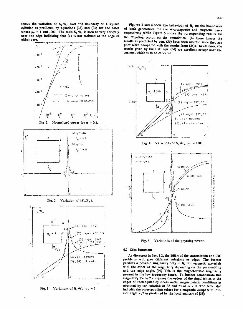
The TM-normalized power loss of a cylindrical conductor, PN , is defined as the ratio between the loss per unit area averaged over the conductor boundary and f€,2/08 where H , is the ampli- tude of the incident field. This loss has been computed for non- magnetic and magnetic cylinders of circular and rectangular crosssections. Typical results are shown in Table 1 and Figure 1. Table 1 compares the analytic solution for a magnetic circular cylinder ( F ~ = 1000) with the numerical solutions of (i) the transmission BIE’s (32, 33) and (ii) the IBC equation (34). As expected, only the exact formulation in terms of equations (32, 33) gives good results in the low frequency region, R q / b = 0.04, where the impedance boundary condition does not apply. How- ever, the exact formulation fails to converge for values of Req/8 of 10 and 1000, while the use of the IBC equation (34) produces very accurate results for these values and in fact for any values of Re, /& greater than 0.1. The results calculated from the numerical solution of the IBC equation (36) also failed to converge in the same regions as the exact formulation and results using this for- mulation are not therefore shown. This is probably because the kernels of equation (36) are very similar to those of equation (33) which are not as well behaved as those of equation (34).

Table 1 IDN for cireoiar geomet5ry yl = 1000.

I I I ‘-

I I I I

I I PN (Analytic)

0.9775 0.1749 1 . 3 8 7 ~ 1 0 - ~ P, (IBC Ext.)

- 0.00006 5.218~10~ PN (2 Eqns.)

0.9778 0.1737 5.149X10-6

Figure 1 shows a plot of PN versus R , b for both nonmag- netic and magnetic cylinders of rectangular crosssection as com- puted from the numerical solution of the exact BIE equations (32, 33) and the IBC equation (34). For the nonmagnetic case, the exact BIE formulation converges over the entire range to the correct solution while the IBC equation gives the proper results only where the IBC applies, namely for values of ReqP greater than about 5. For the magnetic case, the exact BIE formulation fails to converge beyond RCqP 1, while the IBC equation (34) converges to the correct results for all values of R q / 6 > 0.1 but gives incorrect results below this value where the IBC is not satisfied. Similar calculations were made for rectangular cylinders having aspect ratios ranging from 0.1 to 10 with similar results except that the break point between the region where the two solutions apply depends upon the aspect ratio.

For the cylinder with edges, equation (1) is not satisfied near the edges and the use of (34) and (36) would be expected to intro- duce some error. This is further demonstrated in Figure 2, which

1839

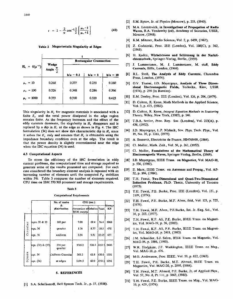
Figures 3 and 4 show the behaviour of H, on the boundaries of both geometries for the non-magnetic and magnetic cases respectively while Figure 5 shows the corresponding results for the Poynting vector on the boundaries. (In these figures the results as predicted by eqn. (36) have been omitted since they are poor when compared with the results from (34)). In all cases, the results given by the IBC eqn. (34) are excellent except near the corners, which is to be expected.

shows the variation of E,/Ht over the boundary of a square cylinder as predicted by equations (32) and (33) for the cases where F~ = 1 and 1ooO. The ratio & / H I is seen to vary abruptly near the edge indicating that (1) is not satisfied at the edge in either case.

Fig. 1 Normalized power for a = 0.1.

t 1 1

Fig. 2 Variation of I Z, 12, I.

Fig. 3 Variations of H , /Hot k, = 1.

0.05-

Fig. 4 Variations of H t / H , , p, = 1000.

Fig. 5 Variations of the poynting power.

4.2 Edge Behavioor

As discussed in Sec. 3.2, the BE’S of the transmission and B C problems will give different solutions at edges. The former predicts a possible singularity only in H , for magnetic materials with the order of the singularity depending on the permeability and the edge angle. [30] This is the magnetostatic singularity present in the low frequency range. To further demonstrate this singularity Table 2 compares the orders of the singularities at the edges of rectangular cylinders under magnetostatic conditions as obtained by the solution of 32 and 33 as o - 0. The table also includes the corresponding values for a magnetic wedge with inte- rior angle n/2as predicted by the local analysis of [31]:

1840

Table 2 Mametostatic Singularity at Edges

I t I I Rectangular Crosssection

1 b/a = 0.1 1 b/a = 1 I b/a = 10

p r = 10

0.423 0.320 0310 0333 p r = 1000

0366 0.286 0.348 0.326 p r = 100

0.160 0.255 0337 0.268

This singularity in H , for magnetic materials is associated with a finite E, and the total power dissipated in the edge region remains finite. As the frequency increases and the effect of the eddy currents dominate, the singularity in H, disappears and is replaced by a dip in H , at the edge as shown in Fig. 4. The IBC formulation (34) does not show this characteristic dip in H , since it solves for E , only and assumes that H , is obtainable using the impedance boundary condition even at the edge. The result is that the power density is slightly overestimated near the edge when the IBC equation (34) is used.

4.3 Computational Aspects

To stress the efficiency of the IBC formulation in eddy current problems, the computational time and storage required to generate some of the results presented are compared. For each case considered the boundary element analysis is repeated with an increasing number of elements until the computed P, stabilizes within 5%. Table 3 compares the number of elements required. CPU time on IBM 370/303 processor and storage requirements,

Table 3

Compotattonrl RcgoIrrmenlr

0

2 1056 430.0 61.8 363.2 LlniformGaussian 3 n . W 7 x' 1056 13593 60.0 12993 at edges q u . (36)

5. REFERENCES

[l] S.A. Scbelkunoff, Bell System Tech. Jr., p. 17, (1938).

[2] S.M. Rytov, Jr. of Physics (Moscow), p. 233, (1940).

[3] M.A. Leontovich, in Investigations of Propagation of Radio Waves, B.A. Vredensky (ed), Academy of Sciencies, USSR, Moscow, (1948).

[4] K.M. Mitzner, Radio ScienceVol. 2, p.4459, (1967).

[5] Z. Godzinski, Proc. IEE (London), Vol. 108(C), p. 362, (1961).

[6] H. Kaden, Wirbelstrome und Schfrmung in der Nachrl- chtentechnik, Springer-Verlag, Berlin, (1959).

[7] J. Lammeraner, M. J. Lammeraner, M. stafl, Eddy Currents, Iliffe, London, (1966).

[8] R.L. Stoll, The Analysis of Eddy Currents, Clarendon Press, London, (1974).

[9] O.V. Tozoni, I.D. Mayergoyz, Analysis of Three Dimen- s i o d Electromagnetic Fields, Technika, Kiev, USSR (1974), p. 259 (in Russian).

[lo] E.M. Deeley, Proc. IEE (London), Vol. 126, p. 204, (1979).

[ll] D. Colton, R. Kress, Math Methods in the Applied Science, Vol. 3, p. 475, (1981).

[12] D. Colton, R. Kress, Integral Equation Methods in Scattering Theory, Wiley, New York, (1983), p. 146.

[13] T.B.A. Senior, Proc. Roy. SOC. (London), Vol. 213(A), p. 436, (1952).

[14] I.D. Mayergoyz, L.P. NIzhnik, Sov. Phys. Tech. Phys., Vol. 19, No. 10, p. 1281, (1975).

[15] A. Bossavit, Electricite de France, HI4769/00, (1984).

[16] CI. Muller, Math. Zeit., Vol. 56, p. 261, (1952).

[17] CI. Muller, Fonndations of the Mathematical Theory of Electromagnetic Waves, Springer-Verlag, Berlin, (1%9).

[18] I.D. Mayergoyz, IEEE Trans. on Magnetics, Vol. MAG-18, p. 536, (1982).

[19] E. Man, IEEE Trans. on Antennas and Propag., Vol. AP- 32, p. 166, (1984).

[20] T.H. Fawzi, Two-Dimensfond and Qaasi-Two-Dhensional Indoction Problems, Ph.D. Thesis, University of Toronto (1973).

[21] T.H. Fawzi, P.E. Burke, Proc. IEE (London), VO%. 121, p. 1109, (1974).

[22] T.H. Fawzi, PE. Burke, M.F. Alves, ibid, Vol. 123, p. 725,

[23] T.H. Fawzi, M.F. Alves, P.E.Burke, Int. Jr. Eng. Sci., vol.

[24] T.H. Fawzi, K.F. Ali, P.E. Burke, IEEE Trans. on Magnet-

[25] T.H. Fawzi, K.F. Ali, P E . Burke, IEEE Trans. on Magnet-

1261 J.M. Schneider, SJ. Salon, IEEE Trans. on Magnetic, Vol.

[27] W.R. Hodgkins, J.F. Waddington, IEEE Trans. on Mag.,

[28] M.G. Andreason, Proc. IEEE, Vol. 53, p. 812, (1965).

[29] T.H. Fawzi, P.E. Burke, M.T. Ahmed, IEEE Trans. on

[30] T.H. Fawzi, M.T. Ahmed, P.E. Burke, Jr. of Applied Phys.,

[31] T.H. Fawzi, P.E. Burke, IEEE Trans. on Mag., Vol. MAG-

(1976).

16, p. 203, (1977).

ics, Vol. MAG-19, p. 36, (1983).

ics, Vol. MAG-19, p. 2401, (1983).

MAG-16, p. 1086, (1980).

VOI. MAG-18, p. 476.

Magnetics, Vol. MAG-20, p. 2010, (1984).

Vol. 57, No. 8, Pt. 11B, p. 3863, (1985).

10, p. 429, (1974).