Embed Size (px)
Citation preview

Online Buy-at-Bulk Network Design
Alina Ene∗ Deeparnab Chakrabarty† Ravishankar Krishnaswamy† Debmalya Panigrahi‡
∗Department of Computer Science and DIMAP, University of Warwick, Coventry, UK.Email: [email protected]
†Microsoft Research, 9 Lavelle Road, Bangalore India.Email: dechakr,[email protected]
‡Department of Computer Science, Duke University, Durham, NC, USA.Email: [email protected]
Abstract
We present the first non-trivial online algorithms for the non-uniform, multicommodity buy-at-bulk (MC-BB) networkdesign problem. Our competitive ratios qualitatively match the best known approximation factors for the corresponding offlineproblems. In particular, we show• A polynomial time online algorithm with a poly-logarithmic competitive ratio for the MC-BB problem in undirected edge-
weighted graphs.• A quasi-polynomial time online algorithm with a poly-logarithmic competitive ratio for the MC-BB problem in undirected
node-weighted graphs.• For any fixed ε > 0, a polynomial time online algorithm with a competitive ratio of O
(k
12+ε) (where k is the number of
demands, and O(.) hides polylog factors) for MC-BB in directed graphs.• Algorithms with matching competitive ratios for the prize-collecting variants of all the above problems.Prior to our work, a logarithmic competitive ratio was known for undirected, edge-weighted graphs only for the special caseof uniform costs (Awerbuch and Azar, FOCS 1997), and a polylogarithmic competitive ratio was known for the edge-weightedsingle-sink problem (Meyerson, SPAA 2004). To the best of our knowledge, no previous online algorithm was known, evenfor uniform costs, in the node-weighted and directed settings.
Our main engine for the results above is an online reduction theorem of MC-BB problems to their single-sink (SS-BB)counterparts. We use the concept of junction-tree solutions (Chekuri et al., FOCS 2006) that play an important role in solvingthe offline versions of the problem via a greedy subroutine – an inherently offline procedure. Our main technical contributionis in designing an online algorithm using only the existence of good junction-trees to reduce an MC-BB instance to multipleSS-BB sub-instances. Along the way, we also give the first non-trivial online node-weighted/directed single-sink buy-at-bulkalgorithms. In addition to the new results, our generic reduction also yields new proofs of recent results for the online node-weighted Steiner forest and online group Steiner forest problems.
Keywords
Online algorithms, network design, multicommodity flows, buy at bulk costs.
I. INTRODUCTION
In a typical network design problem, one has to find a minimum cost (sub) network satisfying various connectivity androuting requirements. These are fundamental problems in combinatorial optimization, operations research, and computerscience. To model economies of scale in network design, Salman et al. [1] proposed the buy-at-bulk framework, which hasbeen studied extensively over the last two decades (e.g., [2], [3], [4], [5], [6], [7], [8], [9]). In this framework, each networkelement is associated with a sub-additive function representing the cost for a given utilization. Given a set of connectivitydemands comprising k source-sink pairs, the goal is to route integral flows from the sources to the corresponding sinksconcurrently to minimize the total cost of the routing.
An important application of the problem is capacity planning in telecommunication networks or in the Internet. Asobserved by Awerbuch and Azar [2], this application is inherently “online” in that terminal-pairs arrive over time and needto be served without knowledge of future pairs. The authors of [2] give a logarithmic-competitive online algorithm for theuniform case where every edge is associated with the same cost function. However, uniformity is not always a feasibleassumption, especially in heterogeneous, dynamic networks like the Internet. Indeed recent research (e.g., [6], [7], [8]) hasfocused on the non-uniform setting with a different sub-additive function for every network element. In this non-uniformsetting, Meyerson [7] gives a polylogarithmic-competitive algorithm for the special case when all terminal-pairs share thesame sink. To the best of our knowledge, no non-trivial online algorithm is known for the general multicommodity setting,which is the focus of our paper.

We consider, in increasing order of generality, undirected edge-weighted graphs, undirected node-weighted graphs, anddirected edge-weighted graphs.1 It is also convenient to classify the problems that we study into the single-sink version whereall the terminal-pairs share a common sink, and the general multicommodity version where the sinks in the terminal-pairsmay be distinct. For notational convenience, we use the following shorthand forms for our problems: X-Y-BB where X= SS or MC (single-sink and multicommodity, respectively) and Y = E or N or D (undirected edge-weighted, undirectednode-weighted, and the general directed case, respectively).
A. Our Contributions
We obtain the following new results (unless otherwise noted, our algorithms run in polynomial time):• A poly-logarithmic competitive online algorithm for the MC-E-BB problem.• A poly-logarithmic competitive online algorithm for MC-N-BB and SS-N-BB that runs in quasi-polynomial time.• An O(k
12+ε)-competitive online algorithm for MC-D-BB for any constant ε > 0 with running time nO(1/ε), where O(.)
hides polylogarithmic factors. For SS-D-BB, the ratio improves to O(kε), translating to a polylogarithmic competitiveratio in quasi-polynomial time.
• Online algorithms for prize-collecting versions of all the above problems with the same competitive ratio.Up to exponents in the logarithm, our online algorithms match the best known offline approximation algorithms (Chekuri etal. [8] for MC-E/N-BB and Antonakopoulos [10] for MC-D-BB); for MC-N-BB, however, a polynomial time, polylogarithmicapproximation is known [9], whereas our algorithm runs in quasi-polynomial time. Furthermore, a logarithmic lower bound,even for SS-E-BB, follows from the lower bound for the online Steiner tree problem [11], and a polylogarithmic lowerbound for online SS-N-BB follows from a matching one for set cover [12].
From a technical perspective, we derive all the multicommodity results using a generic online reduction theorem thatreduces a multicommodity instance to several single-sink instances, for which we either use existing online algorithms orgive new online algorithms. Informally, one can view this as the “online analog” of the junction-tree approach pioneered byChekuri et al. [8] for offline multicommodity network design. We discuss this approach in the next subsection.
B. An Online Reduction to Single Sink Instances
Multicommodity network design problems, both online and offline, are typically more challenging than their single-sinkcounterparts, and have historically2 required new ideas every time depending on the specific problem at hand. The situationis no different for buy-at-bulk, both for uniform and non-uniform costs.
In the offline buy-at-bulk setting, this shortcoming is addressed by Chekuri et al. [8] (expanded to other problems by [9],[16], [10]), who introduce a generic combinatorial framework for mapping a single instance of a multicommodity problemto multiple instances of the corresponding single-sink problem. At the heart of this scheme is the following observation thatholds for many multicommodity problems such as (edge/node) Steiner forest, directed Steiner network, buy-at-bulk, andset connectivity: there exists a near-optimal3 junction-tree solution for the multicommodity problem that decomposes intosolutions to multiple single-sink problems where each single-sink problem connects some subset of the original terminal-pairsto a particular root.
The problem now reduces to finding good junction-trees to cover all the terminal-pairs. The offline techniques [8], [16],[10] tackle this using a greedy algorithm for finding the single-sink solutions; more precisely, in each step they find the bestdensity (cost per terminal-pair) solution that routes a subset of terminal-pairs via a single sink. A set cover style analysis thenbounds the loss for repeating this procedure until all terminal-pairs are covered. However, as the reader may have alreadynoticed, the greedy optimization approach is inherently offline, as finding the best-density solution requires knowledge ofall terminal-pairs upfront. Our main technical contribution in this work is an online version of the junction-tree framework.Indeed, we show how to reduce any multicommodity buy-at-bulk instance to a collection of single-sink instances online.(Informal Theorem) If the junction-tree approximation factor of the MC-BB problem is α, the integrality gap of a naturalLP relaxation of the SS-BB problem is β, and there is a γ-competitive online algorithm for the SS-BB problem, then thereis an O(αβγ · polylog(n))-competitive algorithm for the MC-BB problem.
To prove the above theorem, we first write a composite-LP, which has (a) an outer-LP comprising assignment variablesthat fractionally assign terminal-pairs to roots, and (b) many inner-LPs which correspond to the natural LP relaxations forthe SS-BB problem for each root and the terminal-pairs fractionally assigned to it by the outer-LP. We then apply the
1In undirected graphs, node costs can simulate edge costs; in directed graphs they are equivalent.2For instance, compare [6] and [13] for the SS-E-BB and MC-E-BB problem, and compare Naor et al. [14] and Hajiaghayi et al. [15] for the online
node-weighted Steiner tree and Steiner forest problem.3We call the quality of such a solution the junction-tree approximation factor; e.g., it is O(logn) for MC-E-BB and MC-N-BB [8]
framework of online primal-dual algorithms (see [17] for instance) to solve the composite-LP online. However, there aretwo main challenges we need to surmount.• First, the existing framework has been mostly applied to purely covering/packing LPs4 and our inner-LPs have both
kinds of constraints, and moreover, there is an outer-LP encapsulating them. We show nonetheless that it can be extendedto solving our LP fractionally up to polylogarithmic factors. Indeed, we use the specific flow-structure of the inner-LP, andeach step of our algorithm solves many (auxiliary) min-cost max-flow problems.• The second difficulty is in rounding this fractional solution online. This is a hard problem, and currently we do not know
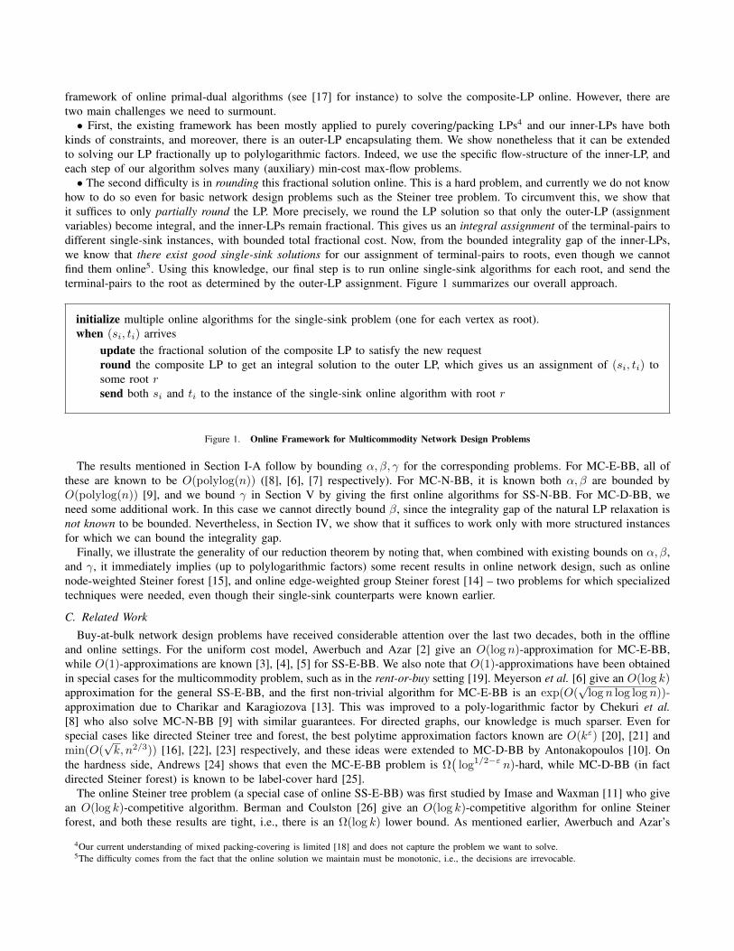
how to do so even for basic network design problems such as the Steiner tree problem. To circumvent this, we show thatit suffices to only partially round the LP. More precisely, we round the LP solution so that only the outer-LP (assignmentvariables) become integral, and the inner-LPs remain fractional. This gives us an integral assignment of the terminal-pairs todifferent single-sink instances, with bounded total fractional cost. Now, from the bounded integrality gap of the inner-LPs,we know that there exist good single-sink solutions for our assignment of terminal-pairs to roots, even though we cannotfind them online5. Using this knowledge, our final step is to run online single-sink algorithms for each root, and send theterminal-pairs to the root as determined by the outer-LP assignment. Figure 1 summarizes our overall approach.
initialize multiple online algorithms for the single-sink problem (one for each vertex as root).when (si, ti) arrives
update the fractional solution of the composite LP to satisfy the new requestround the composite LP to get an integral solution to the outer LP, which gives us an assignment of (si, ti) tosome root rsend both si and ti to the instance of the single-sink online algorithm with root r
Figure 1. Online Framework for Multicommodity Network Design Problems
The results mentioned in Section I-A follow by bounding α, β, γ for the corresponding problems. For MC-E-BB, all ofthese are known to be O(polylog(n)) ([8], [6], [7] respectively). For MC-N-BB, it is known both α, β are bounded byO(polylog(n)) [9], and we bound γ in Section V by giving the first online algorithms for SS-N-BB. For MC-D-BB, weneed some additional work. In this case we cannot directly bound β, since the integrality gap of the natural LP relaxation isnot known to be bounded. Nevertheless, in Section IV, we show that it suffices to work only with more structured instancesfor which we can bound the integrality gap.
Finally, we illustrate the generality of our reduction theorem by noting that, when combined with existing bounds on α, β,and γ, it immediately implies (up to polylogarithmic factors) some recent results in online network design, such as onlinenode-weighted Steiner forest [15], and online edge-weighted group Steiner forest [14] – two problems for which specializedtechniques were needed, even though their single-sink counterparts were known earlier.
C. Related Work
Buy-at-bulk network design problems have received considerable attention over the last two decades, both in the offlineand online settings. For the uniform cost model, Awerbuch and Azar [2] give an O(log n)-approximation for MC-E-BB,while O(1)-approximations are known [3], [4], [5] for SS-E-BB. We also note that O(1)-approximations have been obtainedin special cases for the multicommodity problem, such as in the rent-or-buy setting [19]. Meyerson et al. [6] give an O(log k)approximation for the general SS-E-BB, and the first non-trivial algorithm for MC-E-BB is an exp(O(
√log n log log n))-
approximation due to Charikar and Karagiozova [13]. This was improved to a poly-logarithmic factor by Chekuri et al.[8] who also solve MC-N-BB [9] with similar guarantees. For directed graphs, our knowledge is much sparser. Even forspecial cases like directed Steiner tree and forest, the best polytime approximation factors known are O(kε) [20], [21] andmin(O(
√k, n2/3)) [16], [22], [23] respectively, and these ideas were extended to MC-D-BB by Antonakopoulos [10]. On
the hardness side, Andrews [24] shows that even the MC-E-BB problem is Ω(
log1/2−ε n)-hard, while MC-D-BB (in factdirected Steiner forest) is known to be label-cover hard [25].
The online Steiner tree problem (a special case of online SS-E-BB) was first studied by Imase and Waxman [11] who givean O(log k)-competitive algorithm. Berman and Coulston [26] give an O(log k)-competitive algorithm for online Steinerforest, and both these results are tight, i.e., there is an Ω(log k) lower bound. As mentioned earlier, Awerbuch and Azar’s
4Our current understanding of mixed packing-covering is limited [18] and does not capture the problem we want to solve.5The difficulty comes from the fact that the online solution we maintain must be monotonic, i.e., the decisions are irrevocable.
algorithm [2] can be seen as an O(log n)-competitive online algorithm for the uniform-cost MC-E-BB. For non-uniform buy-at-bulk, the only online algorithm that we are aware of is Meyerson’s [7] polylog-competitive algorithm for the single-sinkproblem. For online node-weighted network design, developments are much more recent. A polylogarithmic approximationfor the node-weighted Steiner tree problem was first given by Naor et al. [14] and later extended to the online node-weightedSteiner forest problem [15] and prize-collecting versions [27]. These algorithms, like ours in this paper, utilize the onlineadaptation of the primal-dual and LP rounding schemas pioneered by the work of Alon et al. [12] for the online set coverproblem (see also [28] for its adaptation to network design problems). We also note that in the node-weighted setting, theonline lower bound can be strengthened to Ω(log n log k) using online set cover lower bounds [12], [29].
II. PRELIMINARIES AND RESULTS
We now formally state the problem, set up notation that we use throughout the paper, and state our main theorems.
A. Our Problems
Buy-at-bulk Network Design. In the most general setting of the MC-D-BB problem, an instance I = (G,X ) consists of adirected graph G = (V,E) and a collection X of terminal-pairs (si, ti) ∈ V × V ; each such si and ti is called a terminal.Each (si, ti) pair also has a positive integer demand di, which we assume to be 1 for clarity in presentation.6 Additionally,each edge e ∈ E is associated with a monotone, sub-additive7 cost function fe : R≥0 → R≥0. A feasible solution to theproblem is a collection of paths P1, . . . , Pk where Pi is a directed path from si to ti carrying load di. Given a solutionP1, . . . , Pk, we let load(e) =
∑i:e∈Pi
di denote the total load on edge e. The goal is to find a feasible solution minimizingthe objective ObjBB :=
∑e∈E fe(load(e)). In the online problem, the offline input consists of the graph G and the cost
functions fe. The pairs (si, ti) arrive online in an unknown, possibly adversarial, order. When a pair (si, ti) arrives, thealgorithm must select the path Pi that connects them, and this decision is irrevocable.
Reduction to the Two-metric Problem. Following previous work, throughout this paper we consider an equivalent problem(up to constant factors) known as two-metric network design. In this problem, instead of functions fe(.) on the edges, weare given two parameters ce and `e on each edge. One can think of ce as a fixed buying cost, or just cost, of edge e, and`e as a per-unit flow cost, or length, of edge e. The feasible solution space is the same as for the buy-at-bulk problem, andthe goal is to minimize the objective Obj2M :=
∑e∈
⋃i Pi
ce +∑i
∑e∈Pi
`e. The following lemma is well known (see e.g.,[8]).
Lemma 1. Given an instance of the buy-at-bulk problem, for any ε > 0 one can find an instance of the two-metric networkdesign problem such that, for any feasible solution, Obj2M ≤ ObjBB ≤ (2 + ε)Obj2M.
Remark. In light of the above lemma, henceforth we abuse notation and let the buy-at-bulk problem mean the two-metricnetwork design problem.
B. Our Tools
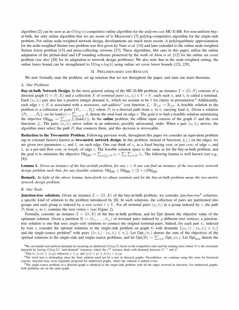
Junction-tree solutions. Given an instance I = (G,X ) of the buy-at-bulk problem, we consider junction-tree8 solutions,a specific kind of solution to the problem introduced by [8]. In such solutions, the collection of pairs are partitioned intogroups and each group is indexed by a root vertex r ∈ V . For all terminal pairs (si, ti) in a group indexed by r, the pathPi from si to ti contains the root vertex r (see Figure 2).
Formally, consider an instance I = (G,X ) of the buy-at-bulk problem, and let Opt denote the objective value of theoptimum solution. Given a partition Π := (πr1 , . . . , πrq ) of terminal pairs indexed by q different root vertices, a junction-tree solution is one that uses single-sink solutions to connect the original terminal-pairs. Indeed, for each part πr indexedby root r, consider the optimal solutions to the single-sink problem on graph G with demands (si, r) : (si, ti) ∈ πrand the single-source problem9 with pairs (r, ti) : (si, ti) ∈ πr. Let Optr(πr) denote the sum of the objectives of theoptimal solutions to the single-sink and single-source problems, and let Opt(Π) :=
∑r∈V Optr(πr). Let Optjunc denote the
6We can handle non-uniform demands by incurring an additional O(logD) factor in the competitive ratio and the running time (where D is the maximumdemand) by having O(logD) “unit-demand” instances, where the ith instance deals with demands between 2i−1 and 2i.
7That is, fe(x) ≥ fe(y) whenever x ≥ y, and fe(x+ y) ≤ fe(x) + fe(y)8The word tree is misleading since the final solution need not be a tree in directed graphs. Nevertheless, we continue using this term for historical
reasons. Junction trees were originally proposed for undirected graphs, where the solution is indeed a tree.9The single-source problem in a directed graph is identical to the single-sink problem with all the edges reversed in direction. For undirected graphs,
both problems are on the same graph.
junctions1
t1
s2
t2
t3
s3
t4
s4
Figure 2. A group of terminal pairs routed via a junction-vertex in an undirected graph.
minimum Opt(Π) over all partitions. We call this solution the optimum junction-tree solution for this instance.10 Clearly,Optjunc ≥ Opt. The junction-tree approximation factor of I is defined to be the ratio Optjunc/Opt.
LP Relaxation. We now describe a natural flow-based LP relaxation for the single-sink buy-at-bulk problem for an instanceI = (G, T ) where T is a set of terminals that need to be connected to the root r.
minimize∑e∈E
cexe +∑i
∑e∈E
`efi(e) (SS-BaB LP)
s.t fi(e) : e ∈ E(G) defines a flow from si to r of value 1 ∀si ∈ Tfi(e) ≤ xe ∀e ∈ Exe ≥ 0, fi(e) ≥ 0 ∀e ∈ E
Recall that the integrality gap of (SS-BaB LP) on the instance I = (G, T ) is defined to be the ratio of Opt to the optimalvalue of the LP (SS-BaB LP). Also, we define the integrality gap for the graph G to be the worst case integrality gap (overall requests T on graph G) of the corresponding instance I = (G, T ).
C. Our Results
Main Technical Theorem and its Applications. Now we are ready to state our main theorem; the proof is in Section III.We say that an online algorithm is γ-competitive for a graph G if, for any sequence of requests X , the online algorithm forbuy-at-bulk returns a solution within a γ-factor of Opt(I), where I = (G,X ).
Theorem 2 (Reduction to Single-Sink Online Algorithms). Fix an instance I = (G,X ) of the MC-BB problem. Supposethe following three conditions hold.
(i) The junction-tree approximation factor of I is at most α.(ii) The integrality gap of (SS-BaB LP) on any single-sink instance on graph G is at most β.(iii) There is a γ-competitive online SS-BB algorithm for any instance on graph G that runs in time T .
Then there is an online algorithm for I running in time poly(n, T ) whose competitive ratio is O(αβγ · polylog(n)).
Using this theorem, we can immediately obtain the following new results mentioned in the introduction.
Theorem 3 (Undirected Edge-weighted Buy-at-Bulk). There is a polylog(n)-competitive, polynomial time randomized onlinealgorithm for the MC-E-BB problem.
Proof: The theorem follows directly by combining Theorem 2 with the following results from previous work. Chekuri etal. [8] prove that the junction-tree approximation factor for the undirected edge-weighted buy-at-bulk problem is O(log k).Chekuri et al. [30] prove that the integrality gap of (SS-BaB LP) in undirected edge-weighted graphs is O(log k). Meyer-son [7] gives a randomized polynomial time online algorithm for the single-sink buy-at-bulk problem with competitive ratioO(log4 n).
Theorem 4 (Undirected Node-weighted Buy-at-Bulk). For any constant ε > 0, there is an O(kεpolylog(n))-competitive,randomized online algorithm for MC-N-BB with running time nO(1/ε). As a corollary, this yields a polylog(n)-competitive,quasi-polynomial time algorithm for this problem.
10Note that copies of the same edge appearing in multiple single-sink solutions are treated as distinct edges in the junction-tree solution. Hence,decomposing the optimal multicommodity solution into its constituent paths does not yield Optjunc = Opt.
Theorem 5 (Directed Buy-at-Bulk). For any constant ε > 0, there is an O(k1/2+εpolylog(n))
)-competitive, polynomial
time online algorithm for the MC-D-BB.
We again use Theorem 2 to prove the above theorems. However, unlike for MC-E-BB, we are not aware of any onlinealgorithms for the SS-N-BB and SS-D-BB problems. We therefore first give online algorithms for these problems, and thenuse Theorem 2; the details appear in Sections V and IV.Finally, we can almost directly use Theorem 2 to also obtain matching results for prize-collecting versions of the aboveproblems. Recall that in a prize-collecting problem, every terminal-pair also comes with a penalty qi, and the algorithm canopt to not satisfy the request by incurring this value in the objective. We give the extension of our results to the correspondingprize-collecting problems in Section VI.
Theorem 6. For each of the above problems, there is an online algorithm with matching running time and competitive ratiofor the corresponding prize-collecting version.
In addition to the new results mentioned above, we can also use Theorem 2 to give alternative proofs (with slightly worsepolylog factors) of some recent results in online network design. By combining Theorem 2 with the polylog(n)-competitivealgorithm for online group Steiner Tree due to Alon et al. [28], we obtain a polylog(n)-competitive online algorithmfor the group Steiner forest problem – a result shown earlier by Naor et al. [14]. Similarly, by combining Theorem 2with the polylog(n)-competitive online algorithm for the node-weighted Steiner tree problem due to Naor et al. [14], weobtain a polylog(n)-competitive online algorithm for the node-weighted Steiner forest problem – a result shown earlier byHajiaghayi et al. [15].Height Reduction Theorem. One of the technical tools that we use repeatedly in this paper is the following result, whichbuilds on the work of Helvig et al. [31]. We give the proof in Section A.
Theorem 7. Given a directed graph G = (V,E) with edge costs ce and lengths `e, for all h > 0, we can efficiently findan upward directed, layered graph Gup
h on (h+ 1) levels and edges (with new costs and lengths) only between successivelevels going from bottom (level h) to top (level 0), such that each layer has n vertices corresponding to the vertices of G,and, for any set of terminals X and any root vertex r,
(i) the optimal objective value of the single-sink buy-at-bulk problem to connect X (at level h) with r (at level 0) onthe graph Gup
h is at most O(hk1/h)φ, where φ is the objective value of an optimal solution of the same instance onthe original graph G;
(ii) given a integral (resp. fractional solution) of objective value φ for the single-sink buy-at-bulk problem to connect Xwith r on the graph Gup
h , we can efficiently recover an integral (resp. fractional solution) of objective value at most φfor the problem on the original graph G.
Likewise, we can obtain a downward directed, layered graph Gdownh on (h+ 1)-levels with edges going from top to bottom,
with the same properties as above except for single-source instances instead.
III. PROOF OF THEOREM 2 (ONLINE REDUCTION TO SINGLE-SINK INSTANCES)
There are three main steps in the proof. In Section III-A, we describe the composite LP which is a relaxation of optimaljunction-tree solutions (for technical reasons, we first need to pre-process the graph). Next, in Section III-B, we show howto fractionally solve the LP online. Third, in Section III-C, we show how to partially round the LP online. The resultingsolution then decomposes as fractional solutions to different single-sink instances. Finally, we use the bounded integralitygap and the online algorithm for SS-BB to wrap up the proof in Section III-D.
A. The Composite-LP Relaxation: MC-BaB LP
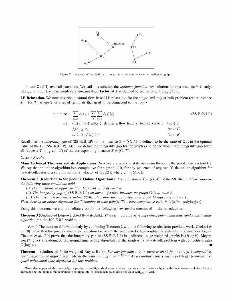
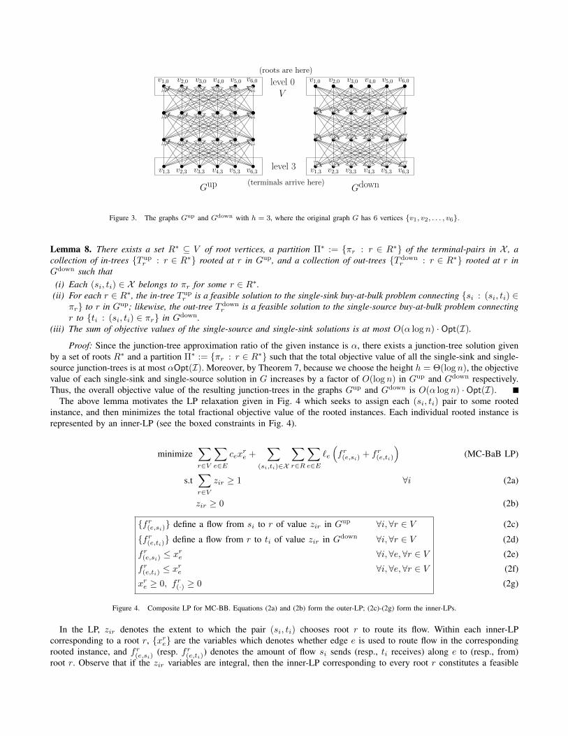
We first apply Theorem 7 with h = Θ(log n) to obtain layered graphs Gup (resp., Gdown) of height O(log n) where allthe edges are directed upward (resp. downward); see Figure 3 for an illustration. The reason for this preprocessing is thatthe length of the (si, ti) paths appear as a factor in our final competitive ratio and the above step bounds it to a logarithmicfactor. Recall that the graph Gup (resp., Gdown) approximately preserves the single-sink (resp., single-source) solutions forany set of terminals and any root. After this step, we can imagine that all the roots (of the single-sink instances we willsolve) are vertices in level 0, and all the terminals will be vertices in level h = Θ(log n). For clarity of presentation, werefer to the root and terminal vertices by the same name in both Gup and Gdown (even though the graphs are completelydisjoint). Overloading notation, let V denote the vertices in level 0 in both Gup and Gdown, and let E be the union of theedge sets of Gup and Gdown. Furthermore, the cost ce and length `e of these edges are inherited from Theorem 7.
Now, using the junction-tree decomposition with approximation factor α, we get the following lemma.
level 0
level 3
Gup
v3,0 v4,0 v5,0 v6,0v1,0 v2,0
v1,3 v2,3 v3,3 v4,3 v5,3 v6,3
V
v3,0 v4,0 v5,0 v6,0v1,0 v2,0
v1,3 v2,3 v3,3 v4,3 v5,3 v6,3
Gdown
(roots are here)
(terminals arrive here)
Figure 3. The graphs Gup and Gdown with h = 3, where the original graph G has 6 vertices v1, v2, . . . , v6.
Lemma 8. There exists a set R∗ ⊆ V of root vertices, a partition Π∗ := πr : r ∈ R∗ of the terminal-pairs in X , acollection of in-trees T up
r : r ∈ R∗ rooted at r in Gup, and a collection of out-trees T downr : r ∈ R∗ rooted at r in
Gdown such that(i) Each (si, ti) ∈ X belongs to πr for some r ∈ R∗.
(ii) For each r ∈ R∗, the in-tree T upr is a feasible solution to the single-sink buy-at-bulk problem connecting si : (si, ti) ∈
πr to r in Gup; likewise, the out-tree T downr is a feasible solution to the single-source buy-at-bulk problem connecting
r to ti : (si, ti) ∈ πr in Gdown.(iii) The sum of objective values of the single-source and single-sink solutions is at most O(α log n) · Opt(I).
Proof: Since the junction-tree approximation ratio of the given instance is α, there exists a junction-tree solution givenby a set of roots R∗ and a partition Π∗ := πr : r ∈ R∗ such that the total objective value of all the single-sink and single-source junction-trees is at most αOpt(I). Moreover, by Theorem 7, because we choose the height h = Θ(log n), the objectivevalue of each single-sink and single-source solution in G increases by a factor of O(log n) in Gup and Gdown respectively.Thus, the overall objective value of the resulting junction-trees in the graphs Gup and Gdown is O(α log n) · Opt(I).
The above lemma motivates the LP relaxation given in Fig. 4 which seeks to assign each (si, ti) pair to some rootedinstance, and then minimizes the total fractional objective value of the rooted instances. Each individual rooted instance isrepresented by an inner-LP (see the boxed constraints in Fig. 4).
minimize∑r∈V
∑e∈E
cexre +
∑(si,ti)∈X
∑r∈R
∑e∈E
`e
(fr(e,si) + fr(e,ti)
)(MC-BaB LP)
s.t∑r∈V
zir ≥ 1 ∀i (2a)
zir ≥ 0 (2b)
fr(e,si) define a flow from si to r of value zir in Gup ∀i,∀r ∈ Vfr(e,ti) define a flow from r to ti of value zir in Gdown ∀i,∀r ∈ Vfr(e,si) ≤ x
re ∀i,∀e,∀r ∈ V
fr(e,ti) ≤ xre ∀i,∀e,∀r ∈ V
xre ≥ 0, fr(·) ≥ 0
(2c)
(2d)
(2e)
(2f)
(2g)
Figure 4. Composite LP for MC-BB. Equations (2a) and (2b) form the outer-LP; (2c)-(2g) form the inner-LPs.
In the LP, zir denotes the extent to which the pair (si, ti) chooses root r to route its flow. Within each inner-LPcorresponding to a root r, xre are the variables which denotes whether edge e is used to route flow in the correspondingrooted instance, and fr(e,si) (resp. fr(e,ti)) denotes the amount of flow si sends (resp., ti receives) along e to (resp., from)root r. Observe that if the zir variables are integral, then the inner-LP corresponding to every root r constitutes a feasible
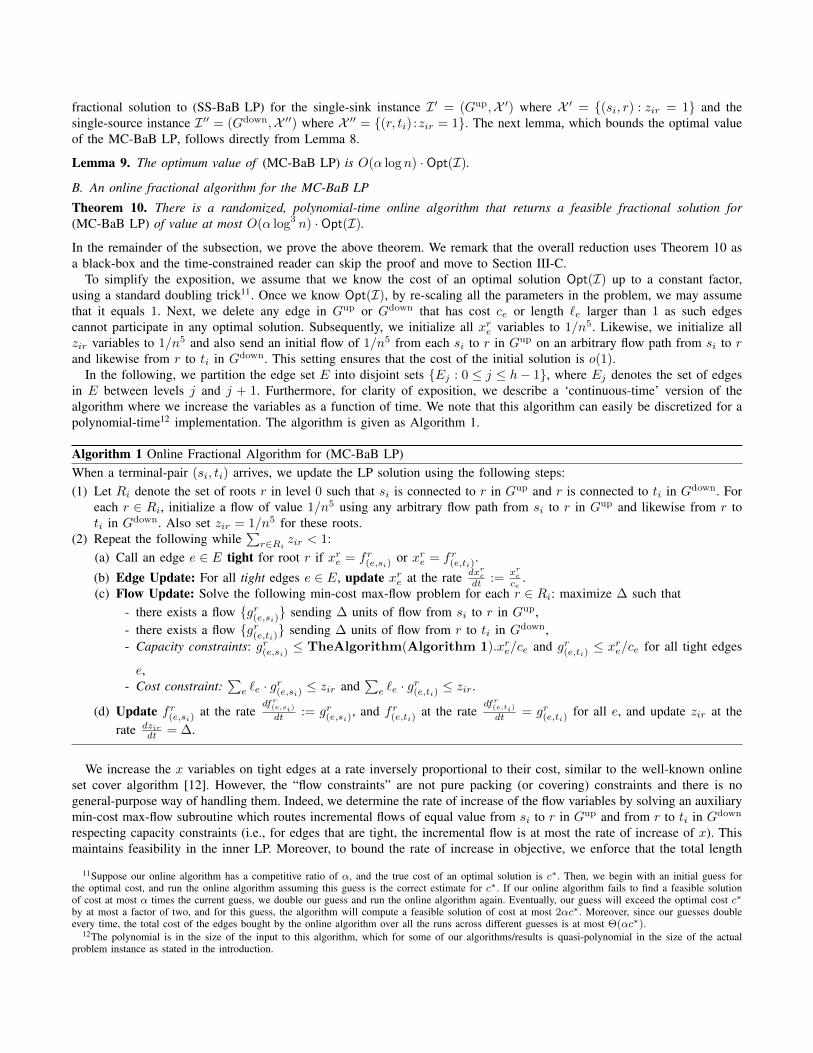
fractional solution to (SS-BaB LP) for the single-sink instance I ′ = (Gup,X ′) where X ′ = (si, r) : zir = 1 and thesingle-source instance I ′′ = (Gdown,X ′′) where X ′′ = (r, ti) :zir = 1. The next lemma, which bounds the optimal valueof the MC-BaB LP, follows directly from Lemma 8.
Lemma 9. The optimum value of (MC-BaB LP) is O(α log n) · Opt(I).
B. An online fractional algorithm for the MC-BaB LP
Theorem 10. There is a randomized, polynomial-time online algorithm that returns a feasible fractional solution for(MC-BaB LP) of value at most O(α log3 n) · Opt(I).
In the remainder of the subsection, we prove the above theorem. We remark that the overall reduction uses Theorem 10 asa black-box and the time-constrained reader can skip the proof and move to Section III-C.
To simplify the exposition, we assume that we know the cost of an optimal solution Opt(I) up to a constant factor,using a standard doubling trick11. Once we know Opt(I), by re-scaling all the parameters in the problem, we may assumethat it equals 1. Next, we delete any edge in Gup or Gdown that has cost ce or length `e larger than 1 as such edgescannot participate in any optimal solution. Subsequently, we initialize all xre variables to 1/n5. Likewise, we initialize allzir variables to 1/n5 and also send an initial flow of 1/n5 from each si to r in Gup on an arbitrary flow path from si to rand likewise from r to ti in Gdown. This setting ensures that the cost of the initial solution is o(1).
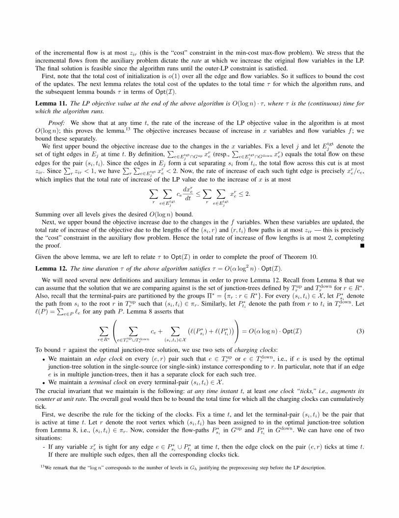
In the following, we partition the edge set E into disjoint sets Ej : 0 ≤ j ≤ h− 1, where Ej denotes the set of edgesin E between levels j and j + 1. Furthermore, for clarity of exposition, we describe a ‘continuous-time’ version of thealgorithm where we increase the variables as a function of time. We note that this algorithm can easily be discretized for apolynomial-time12 implementation. The algorithm is given as Algorithm 1.
Algorithm 1 Online Fractional Algorithm for (MC-BaB LP)When a terminal-pair (si, ti) arrives, we update the LP solution using the following steps:(1) Let Ri denote the set of roots r in level 0 such that si is connected to r in Gup and r is connected to ti in Gdown. For
each r ∈ Ri, initialize a flow of value 1/n5 using any arbitrary flow path from si to r in Gup and likewise from r toti in Gdown. Also set zir = 1/n5 for these roots.
(2) Repeat the following while∑r∈Ri
zir < 1:(a) Call an edge e ∈ E tight for root r if xre = fr(e,si) or xre = fr(e,ti).
(b) Edge Update: For all tight edges e ∈ E, update xre at the rate dxre
dt :=xre
ce.
(c) Flow Update: Solve the following min-cost max-flow problem for each r ∈ Ri: maximize ∆ such that- there exists a flow gr(e,si) sending ∆ units of flow from si to r in Gup,- there exists a flow gr(e,ti) sending ∆ units of flow from r to ti in Gdown,- Capacity constraints: gr(e,si) ≤ TheAlgorithm(Algorithm 1).xre/ce and gr(e,ti) ≤ xre/ce for all tight edges
e,- Cost constraint:
∑e `e · gr(e,si) ≤ zir and
∑e `e · gr(e,ti) ≤ zir.
(d) Update fr(e,si) at the ratedfr
(e,si)
dt := gr(e,si), and fr(e,ti) at the ratedfr
(e,ti)
dt = gr(e,ti) for all e, and update zir at therate dzir
dt = ∆.
We increase the x variables on tight edges at a rate inversely proportional to their cost, similar to the well-known onlineset cover algorithm [12]. However, the “flow constraints” are not pure packing (or covering) constraints and there is nogeneral-purpose way of handling them. Indeed, we determine the rate of increase of the flow variables by solving an auxiliarymin-cost max-flow subroutine which routes incremental flows of equal value from si to r in Gup and from r to ti in Gdown
respecting capacity constraints (i.e., for edges that are tight, the incremental flow is at most the rate of increase of x). Thismaintains feasibility in the inner LP. Moreover, to bound the rate of increase in objective, we enforce that the total length
11Suppose our online algorithm has a competitive ratio of α, and the true cost of an optimal solution is c∗. Then, we begin with an initial guess forthe optimal cost, and run the online algorithm assuming this guess is the correct estimate for c∗. If our online algorithm fails to find a feasible solutionof cost at most α times the current guess, we double our guess and run the online algorithm again. Eventually, our guess will exceed the optimal cost c∗by at most a factor of two, and for this guess, the algorithm will compute a feasible solution of cost at most 2αc∗. Moreover, since our guesses doubleevery time, the total cost of the edges bought by the online algorithm over all the runs across different guesses is at most Θ(αc∗).
12The polynomial is in the size of the input to this algorithm, which for some of our algorithms/results is quasi-polynomial in the size of the actualproblem instance as stated in the introduction.
of the incremental flow is at most zir (this is the “cost” constraint in the min-cost max-flow problem). We stress that theincremental flows from the auxiliary problem dictate the rate at which we increase the original flow variables in the LP.The final solution is feasible since the algorithm runs until the outer-LP constraint is satisfied.
First, note that the total cost of initialization is o(1) over all the edge and flow variables. So it suffices to bound the costof the updates. The next lemma relates the total cost of the updates to the total time τ for which the algorithm runs, andthe subsequent lemma bounds τ in terms of Opt(I).
Lemma 11. The LP objective value at the end of the above algorithm is O(log n) · τ , where τ is the (continuous) time forwhich the algorithm runs.
Proof: We show that at any time t, the rate of the increase of the LP objective value in the algorithm is at mostO(log n); this proves the lemma.13 The objective increases because of increase in x variables and flow variables f ; webound these separately.
We first upper bound the objective increase due to the changes in the x variables. Fix a level j and let Etgtj denote the
set of tight edges in Ej at time t. By definition,∑e∈Etgt
j ∩Gup xre (resp.,∑e∈Etgt
j ∩Gdown xre) equals the total flow on theseedges for the pair (si, ti). Since the edges in Ej form a cut separating si from ti, the total flow across this cut is at mostzir. Since
∑r zir < 1, we have
∑r
∑e∈Etgt
jxre < 2. Now, the rate of increase of each such tight edge is precisely xre/ce,
which implies that the total rate of increase of the LP value due to the increase of x is at most∑r
∑e∈Etgt
j
cedxredt≤∑r
∑e∈Etgt
j
xre ≤ 2.
Summing over all levels gives the desired O(log n) bound.Next, we upper bound the objective increase due to the changes in the f variables. When these variables are updated, the
total rate of increase of the objective due to the lengths of the (si, r) and (r, ti) flow paths is at most zir — this is preciselythe “cost” constraint in the auxiliary flow problem. Hence the total rate of increase of flow lengths is at most 2, completingthe proof.
Given the above lemma, we are left to relate τ to Opt(I) in order to complete the proof of Theorem 10.
Lemma 12. The time duration τ of the above algorithm satisfies τ = O(α log2 n) · Opt(I).
We will need several new definitions and auxiliary lemmas in order to prove Lemma 12. Recall from Lemma 8 that wecan assume that the solution that we are comparing against is the set of junction-trees defined by T up
r and T downr for r ∈ R∗.
Also, recall that the terminal-pairs are partitioned by the groups Π∗ = πr : r ∈ R∗. For every (si, ti) ∈ X , let P ∗si denotethe path from si to the root r in T up
r such that (si, ti) ∈ πr. Similarly, let P ∗ti denote the path from r to ti in T downr . Let
`(P ) =∑e∈P `e for any path P . Lemma 8 asserts that
∑r∈R∗
∑e∈Tup
r ∪Tdownr
ce +∑
(si,ti)∈X
(`(P ∗si) + `(P ∗ti)
) = O(α log n) · Opt(I) (3)
To bound τ against the optimal junction-tree solution, we use two sets of charging clocks:• We maintain an edge clock on every (e, r) pair such that e ∈ T up
r or e ∈ T downr , i.e., if e is used by the optimal
junction-tree solution in the single-source (or single-sink) instance corresponding to r. In particular, note that if an edgee is in multiple junction-trees, then it has a separate clock for each such tree.
• We maintain a terminal clock on every terminal-pair (si, ti) ∈ X .The crucial invariant that we maintain is the following: at any time instant t, at least one clock “ticks,” i.e., augments itscounter at unit rate. The overall goal would then be to bound the total time for which all the charging clocks can cumulativelytick.
First, we describe the rule for the ticking of the clocks. Fix a time t, and let the terminal-pair (si, ti) be the pair thatis active at time t. Let r denote the root vertex which (si, ti) has been assigned to in the optimal junction-tree solutionfrom Lemma 8, i.e., (si, ti) ∈ πr. Now, consider the flow-paths P ∗si in Gup and P ∗ti in Gdown. We can have one of twosituations:
- If any variable xre is tight for any edge e ∈ P ∗si ∪ P ∗ti at time t, then the edge clock on the pair (e, r) ticks at time t.If there are multiple such edges, then all the corresponding clocks tick.
13We remark that the “logn” corresponds to the number of levels in Gh justifying the preprocessing step before the LP description.
- Otherwise, both paths are free of tight edges. In this case, the terminal clock for (si, ti) ticks at time t.
Lemma 13. For any pair (e, r) such that e ∈ T upr ∪ T down
r , its edge clock ticks for O(ce log n) time.
Proof: Notice that xre is initialized to 1/n5 for all roots r, and increases at the rate
dxredt
=xrece
(4)
at all times when the edge clock on (e, r) ticks. To see why, consider a time t when the clock on (e, r) ticks, and let(si, ti) denote the active terminal-pair at time t. It must be that (i) (si, ti) has been assigned to root r in Π∗, and (ii) eitherxre = fr(e,si) or xre = fr(e,ti). But in this case, we increase such variables at rate xre/ce in our algorithm (Step (2a)). Therefore,we can infer that the value of xre would be 1 after the edge clock on e has ticked for time O(ce log n). But clearly, e cannotbe a tight edge for any subsequent terminal-pair (si, ti) once xe reaches 1; therefore, the edge clock on (e, r) ticks forO(ce log n) time overall.
Lemma 14. For every terminal-pair (si, ti) connected by the optimal junction-tree solution through the root vertex r, thetotal time for which the terminal clock ticks is at most O(log n) ·max(`(P ∗si), `(P
∗ti)).
Proof: Recall that if the terminal clock for (si, ti) is ticking at time t, then it must mean that no edge is tight on eitherpath P ∗si or P ∗ti . In this case, we show that the variable zir increases at a fast enough rate, where r is the root (si, ti) isassigned to in the optimal junction-tree, i.e., (si, ti) ∈ πr. We show this by exhibiting a feasible solution to the auxiliaryLP considered in Step (2b) of the algorithm for root r. Indeed, send the flow from si to r along P ∗si , and likewise from rto ti along P ∗ti . Also set the value of ∆ to be zir/max(`(P ∗si), `(P
∗ti)). Clearly, on the edges of these flow paths, we do
not have any capacity constraints since no edge is tight. So, the only constraints are the cost constraints which are satisfiedby the choice of ∆. Hence, the rate of increase of zir is at least
dzirdt≥ zir
max(`(P ∗si), `(P∗ti))
(5)
at all times when the terminal clock on (si, ti) ticks. This proves the claim, for otherwise the variable zir would have reached1, and the algorithm would have completed processing (si, ti).
Since at least one clock ticks at all times, the total time clocked is at least τ , the duration of the algorithm. Lemma 13and Lemma 14 imply that
τ ≤ O(log n)∑r∈R∗
∑e∈Tup
r ∪Tdownr
ce +∑
(si,ti)∈X
(`(P ∗si) + `(P ∗ti)
)which together with (3) completes the proof of Lemma 12. Theorem 10 follows from Lemma 11 and Lemma 12.
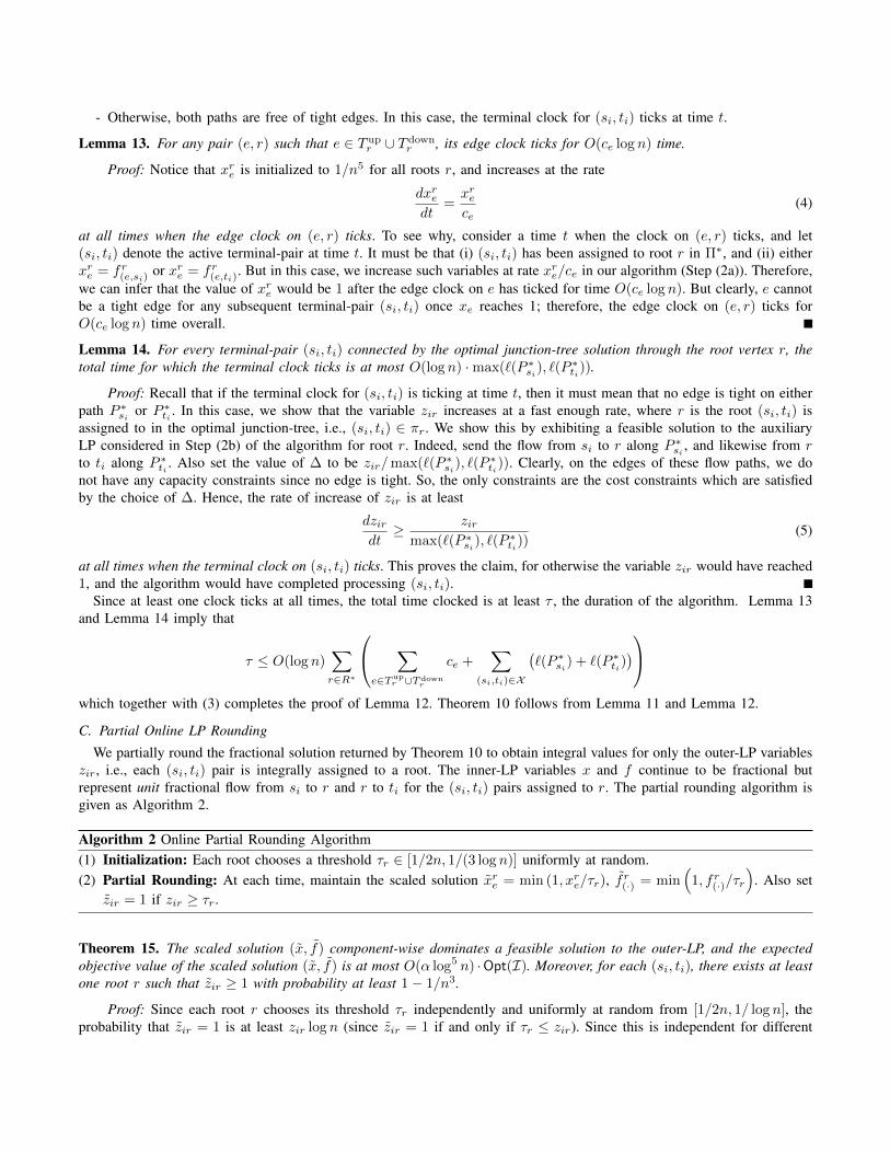
C. Partial Online LP Rounding
We partially round the fractional solution returned by Theorem 10 to obtain integral values for only the outer-LP variableszir, i.e., each (si, ti) pair is integrally assigned to a root. The inner-LP variables x and f continue to be fractional butrepresent unit fractional flow from si to r and r to ti for the (si, ti) pairs assigned to r. The partial rounding algorithm isgiven as Algorithm 2.
Algorithm 2 Online Partial Rounding Algorithm(1) Initialization: Each root chooses a threshold τr ∈ [1/2n, 1/(3 log n)] uniformly at random.(2) Partial Rounding: At each time, maintain the scaled solution xre = min (1, xre/τr), fr(·) = min
(1, fr(·)/τr
). Also set
zir = 1 if zir ≥ τr.
Theorem 15. The scaled solution (x, f) component-wise dominates a feasible solution to the outer-LP, and the expectedobjective value of the scaled solution (x, f) is at most O(α log5 n) ·Opt(I). Moreover, for each (si, ti), there exists at leastone root r such that zir ≥ 1 with probability at least 1− 1/n3.
Proof: Since each root r chooses its threshold τr independently and uniformly at random from [1/2n, 1/ log n], theprobability that zir = 1 is at least zir log n (since zir = 1 if and only if τr ≤ zir). Since this is independent for different
roots, a standard Chernoff-Hoeffding bound application (see, e.g., [32]) shows that each (si, ti) pair has zir = 1 for someroot r with probability at least 1− 1/n3. Moreover, the expected value of any variable xre is given by
E [xre] ≤∫ logn
τr=1/2n
xreτr
log ndτr ≤ O(log2 n)xre.
A similar argument shows that the expected values of scaled flow variables are also bounded by O(log2 n) times their valuesin the fractional solution. This shows that the expected objective value of the (x, f) solution is at most O(log2 n) times thevalue of (x, f); by Theorem 10, the latter is at most O(α log3 n)Opt(I). Combining these facts gives us the desired boundon the value of the scaled solution.
It remains to show that the scaled solution dominates a feasible solution to the LP. To this end, fix some root r and letXr denote the set of (si, ti) pairs for which zir = 1. We need to show that installing capacities of fr(e,si) on the edgescan support unit flow from si to r in Gup for all (si, ti) ∈ Xr. Suppose for contradiction that there is is a cut Q separatingsi from r of capacity strictly smaller than 1. This implies that every edge e ∈ Q must have fr(e,si) ≤ τr; otherwise, wewould have an edge e with fr(e,si) = 1, which contradicts our assumption on the cut capacity. But then the value of the
min-cut is precisely(∑
e∈Q fr(e,si)
)/τr, which must be at least 1 because of the following two observations: (i) we know
that fr(e,si) is a feasible flow from si to r of value zir and hence it must be that∑e∈Q f
r(e,si)
≥ zir, and (ii) since zir = 1,it must be that zir ≥ τr. This contradicts the assumption that the cut capacity is strictly smaller than 1. A similar argumentshows that the variables fr(e,ti) can support unit flow from r to ti for every (si, ti) with zir = 1.
D. Wrapping up: Invoking the Single-Sink Online Algorithm
We are now ready to put all the pieces together and present our overall online multicommodity buy-at-bulk algorithm asAlgorithm 3. SingleSinkAlg is the online algorithm for SS-BB alluded to in point (iii) of the statement of Theorem 2.
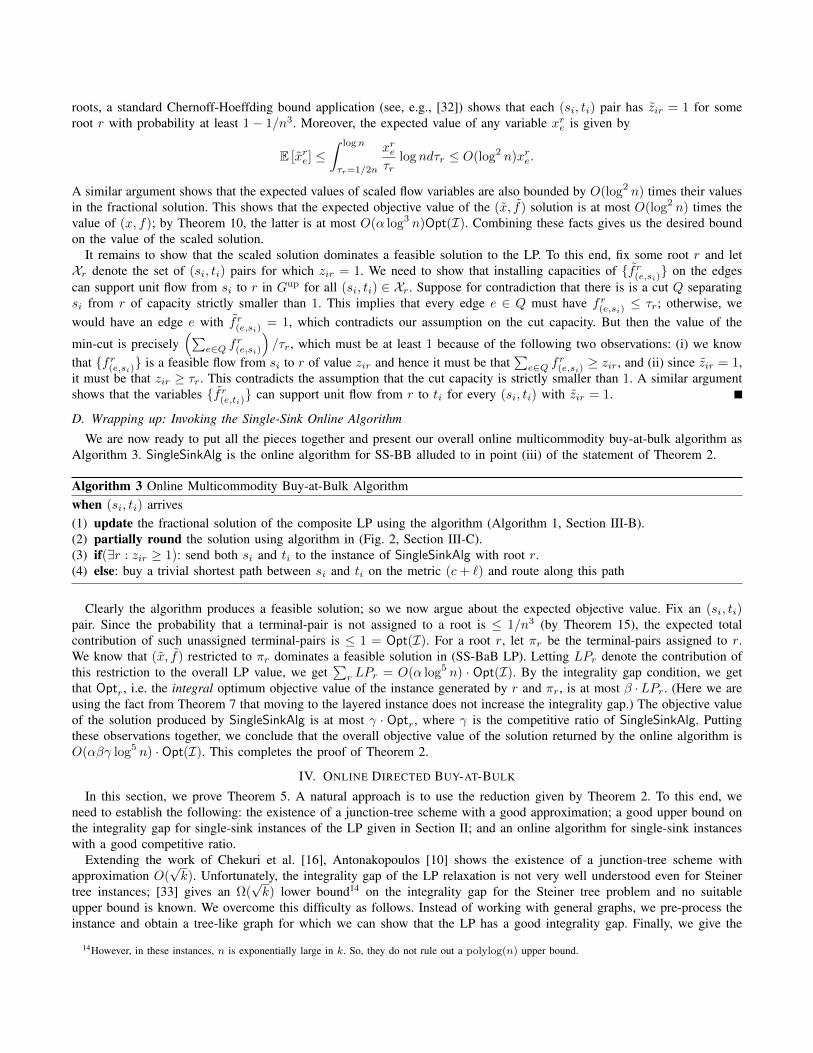
Algorithm 3 Online Multicommodity Buy-at-Bulk Algorithmwhen (si, ti) arrives(1) update the fractional solution of the composite LP using the algorithm (Algorithm 1, Section III-B).(2) partially round the solution using algorithm in (Fig. 2, Section III-C).(3) if(∃r : zir ≥ 1): send both si and ti to the instance of SingleSinkAlg with root r.(4) else: buy a trivial shortest path between si and ti on the metric (c+ `) and route along this path
Clearly the algorithm produces a feasible solution; so we now argue about the expected objective value. Fix an (si, ti)pair. Since the probability that a terminal-pair is not assigned to a root is ≤ 1/n3 (by Theorem 15), the expected totalcontribution of such unassigned terminal-pairs is ≤ 1 = Opt(I). For a root r, let πr be the terminal-pairs assigned to r.We know that (x, f) restricted to πr dominates a feasible solution in (SS-BaB LP). Letting LPr denote the contribution ofthis restriction to the overall LP value, we get
∑r LPr = O(α log5 n) · Opt(I). By the integrality gap condition, we get
that Optr, i.e. the integral optimum objective value of the instance generated by r and πr, is at most β ·LPr. (Here we areusing the fact from Theorem 7 that moving to the layered instance does not increase the integrality gap.) The objective valueof the solution produced by SingleSinkAlg is at most γ · Optr, where γ is the competitive ratio of SingleSinkAlg. Puttingthese observations together, we conclude that the overall objective value of the solution returned by the online algorithm isO(αβγ log5 n) · Opt(I). This completes the proof of Theorem 2.
IV. ONLINE DIRECTED BUY-AT-BULK
In this section, we prove Theorem 5. A natural approach is to use the reduction given by Theorem 2. To this end, weneed to establish the following: the existence of a junction-tree scheme with a good approximation; a good upper bound onthe integrality gap for single-sink instances of the LP given in Section II; and an online algorithm for single-sink instanceswith a good competitive ratio.
Extending the work of Chekuri et al. [16], Antonakopoulos [10] shows the existence of a junction-tree scheme withapproximation O(
√k). Unfortunately, the integrality gap of the LP relaxation is not very well understood even for Steiner
tree instances; [33] gives an Ω(√k) lower bound14 on the integrality gap for the Steiner tree problem and no suitable
upper bound is known. We overcome this difficulty as follows. Instead of working with general graphs, we pre-process theinstance and obtain a tree-like graph for which we can show that the LP has a good integrality gap. Finally, we give the
14However, in these instances, n is exponentially large in k. So, they do not rule out a polylog(n) upper bound.
T upr1
· · ·
T downr1
· · ·
T upr2 T down
r2
r1 r2
s1 s2 sk t1 t2 tk
r2 r2
Figure 5. Construction of graph H .
first non-trivial online algorithm for the directed single-sink buy-at-bulk problem. These results, together with our reduction(Theorem 2), imply the online algorithm for MC-D-BB.
We devote the rest of this section to the proof of Theorem 5; to aid the reader, we restate the theorem below.
Theorem 16. For any constant ε > 0, there is a O(k12+εpolylog(n))-competitive, polynomial time randomized online
algorithm for the general buy-at-bulk problem.
Pre-processing step. We first give our reduction from general instances of the directed buy-at-bulk problem to much morestructured instances; the reduction loses a factor of O(k
12+ε) in the approximation ratio.
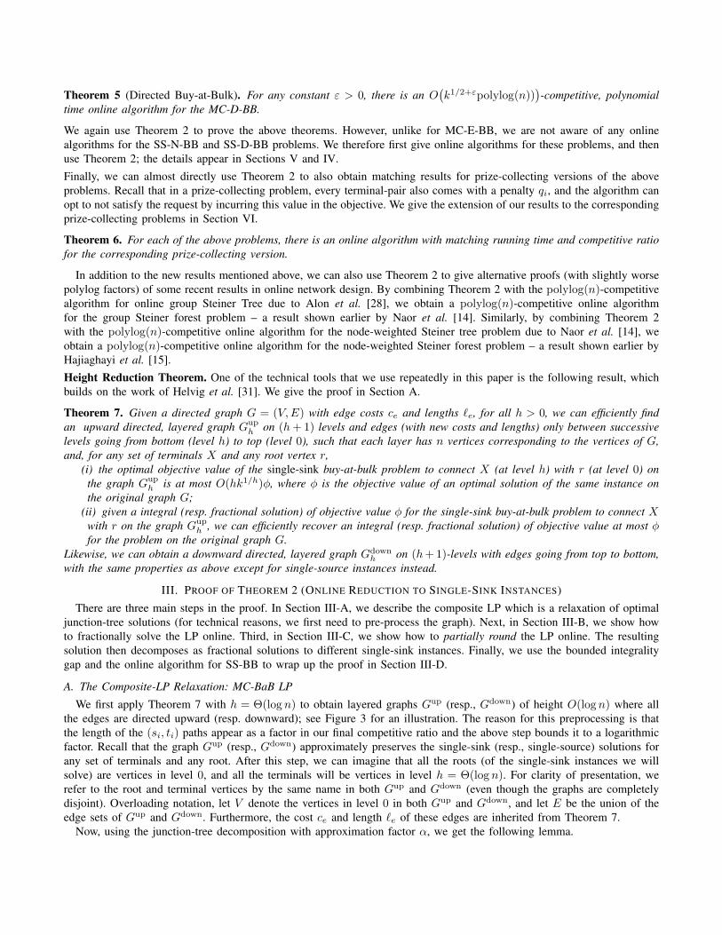
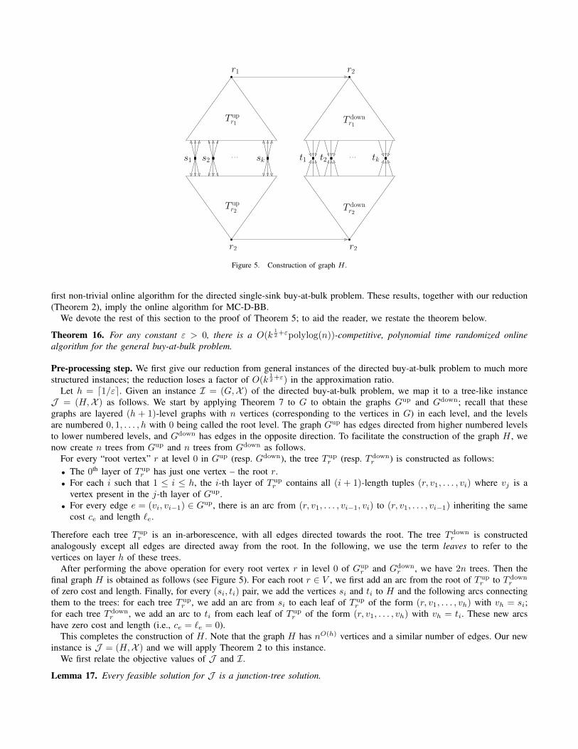
Let h = d1/εe. Given an instance I = (G,X ) of the directed buy-at-bulk problem, we map it to a tree-like instanceJ = (H,X ) as follows. We start by applying Theorem 7 to G to obtain the graphs Gup and Gdown; recall that thesegraphs are layered (h + 1)-level graphs with n vertices (corresponding to the vertices in G) in each level, and the levelsare numbered 0, 1, . . . , h with 0 being called the root level. The graph Gup has edges directed from higher numbered levelsto lower numbered levels, and Gdown has edges in the opposite direction. To facilitate the construction of the graph H , wenow create n trees from Gup and n trees from Gdown as follows.
For every “root vertex” r at level 0 in Gup (resp. Gdown), the tree T upr (resp. T down
r ) is constructed as follows:• The 0th layer of T up
r has just one vertex – the root r.• For each i such that 1 ≤ i ≤ h, the i-th layer of T up
r contains all (i + 1)-length tuples (r, v1, . . . , vi) where vj is avertex present in the j-th layer of Gup.
• For every edge e = (vi, vi−1) ∈ Gup, there is an arc from (r, v1, . . . , vi−1, vi) to (r, v1, . . . , vi−1) inheriting the samecost ce and length `e.
Therefore each tree T upr is an in-arborescence, with all edges directed towards the root. The tree T down
r is constructedanalogously except all edges are directed away from the root. In the following, we use the term leaves to refer to thevertices on layer h of these trees.
After performing the above operation for every root vertex r in level 0 of Gupr and Gdown
r , we have 2n trees. Then thefinal graph H is obtained as follows (see Figure 5). For each root r ∈ V , we first add an arc from the root of T up
r to T downr
of zero cost and length. Finally, for every (si, ti) pair, we add the vertices si and ti to H and the following arcs connectingthem to the trees: for each tree T up
r , we add an arc from si to each leaf of T upr of the form (r, v1, . . . , vh) with vh = si;
for each tree T downr , we add an arc to ti from each leaf of T up
r of the form (r, v1, . . . , vh) with vh = ti. These new arcshave zero cost and length (i.e., ce = `e = 0).
This completes the construction of H . Note that the graph H has nO(h) vertices and a similar number of edges. Our newinstance is J = (H,X ) and we will apply Theorem 2 to this instance.
We first relate the objective values of J and I.
Lemma 17. Every feasible solution for J is a junction-tree solution.
Proof: Note that any (si, ti) path in H has the following structure: si connects to a leaf node of T upr for some r ∈ V ,
then continues to the root r, then traverse the edge to the root of T downr , then goes down to a leaf of T down
r and finallyconnects to ti. Thus, for any feasible solution for J , the (si, ti) pairs can be partitioned based on the root r through whichthey connect.
Lemma 18. Any feasible solution for J can be mapped to a feasible solution — in fact, a junction-tree solution — for Iof equal or smaller objective value.
Proof: Note that from the previous lemma, any feasible solution S in J is a junction-tree solution. Therefore, there isa partition ΠS of the (si, ti) pairs depending on which root vertex they are using to connect. Moreover, it follows from ourconstruction of the trees in H that any edge in T up
r (resp. T downr ) corresponds to an edge in Gup (resp. Gdown). Therefore,
if we map each edge appearing in solution S to its corresponding edge in Gup or Gdown, we obtain a mapping from eachjunction tree of S rooted at r to a junction tree in Gup ∪ Gdown rooted at r that is connecting the same subset of pairs.Finally, by Theorem 7, each junction tree in Gup∪Gdown rooted at r can be mapped, without increasing the objective value,to a junction tree in G rooted at r that is connecting the same subset of pairs. This completes the proof of the lemma.
Lemma 19. Opt(J ) ≤ O(hk1/h)Optjunc(I), where Optjunc(I) is the objective value of an optimal junction-tree solutionfor I.
Proof: Consider the optimal junction tree solution for I. Let the optimum partition be Π = (πr1 , . . . , πrq ) whereR∗ = r1, r2, . . . , rq is the set of roots of the junction trees. For each r ∈ R∗, let Xr = si : (si, ti) ∈ πr be the setof sources of πr and Yr be the corresponding sinks. From Theorem 7, we know that the optimum objective value of anyone single-sink problem connecting Xr to r in Gup is at most O(hk1/h) times the objective value of the optimum solutionconnecting each source in Xr to r. An analogous upper bound holds for every optimal single-source solution connecting rto each sink in Yr. Therefore, we get that the total sum of objective values of each of the junction trees in Gup and Gdown isat most O(hk1/h)Optjunc(I). Now notice that any solution SG for (Gup, Xr) can easily be “simulated” by a solution ST inthe tree T up
r : indeed, for every root-vertex path (r, v1, v2, . . . , vi) in the solution SG, include the edge from (r, v1, v2, . . . , vi)to (r, v1, v2, . . . , vi−1) in ST (recall the vertices in T up
r exactly correspond to such root-vertex paths). It is easy to see thatthe objective value of the solution ST in T up
r is the same as that of SG. Similarly, any solution for (Gdown, Yr) can besimulated in T down
r with the same objective value. It follows that there is a feasible solution in J of objective value at mostO(hk1/h)Optjunc(I).
Corollary 20. Opt(J ) ≤ O(k12+ε)Opt(I).
Proof Sketch: Antonakopoulos [10] shows that there exists a junction-tree solution of cost at most O(√k)Opt(I). The
corollary follows from this work and the fact that we set h = Θ(1/ε).
Now we are ready to show that the new instance J has the properties required by the reduction, i.e., Theorem 2 can beapplied. In the following lemma, a single-source (resp. single-sink) sub-instance J ′ = (H, T , v) of J = (H,X ) is a single-source (resp. single-sink) instance of the following form: the graph is the same as in J , namely H; the set of terminals T isa subset of the sources (resp. sinks) of X ; the terminals T need to be connected to a root vertex v ∈ V (H)\si, ti : i ∈ [k].Lemma 21. Let J be the instance described above. Let α, β, γ be as in the statement of Theorem 2. We have
(i) The junction-tree approximation factor of J is 1 (i.e., α = 1).(ii) The integrality gap of (SS-BaB LP) for any single-sink/source sub-instance J ′ = (H, T , v) is O(h log n log k) (i.e.,
β = O(h log n log k)).(iii) There is a O(h2 log2 n log k)-competitive algorithm for any single-sink/source sub-instance J ′ = (H, T , v) (i.e., γ =
O(h2 log2 n log k)).
Proof: Property (i) follows from Lemma 17. Thus we focus on proving (ii) and (iii). In the following, we assume thatwe are working with a single-sink sub-instance J ′ of J ; the proof is very similar for single-source sub-instances and weomit it.
In order to show (ii) and (iii), we will map the sub-instance J ′ = (H, T , v) to an instance of the group Steiner treeproblem on a tree as follows. Since v ∈ V (H) \ si, ti : i ∈ [k], we have v ∈ T up
r ∪ T downr for some r. We first consider
the case when v ∈ T upr . In order to define the tree of the group Steiner tree instance, we start with the subtree Tv of T up
r
rooted at v. We add the following ‘dangling’ edges to Tv for each source si ∈ T : for each leaf vertex u ∈ T upr such that
si has an edge in T upr to u, we add a new vertex u′ to Tv and connect it to u. Let T be the resulting tree. We assign
weights to the edges of T as follows. Each of the old edges e ∈ Tv receives a weight equal to ce. Each of the new edges
uu′ ∈ E(T ) \ E(Tv) receives a weight equal to `(Pu), where Pu is the path of T upr from u to v. Finally, we define the
following groups: for each source si ∈ T , we introduce a group Si consisting of all the new vertices u′ ∈ V (T ) \ V (Tv)such that si is connected to its partner u in T up
r (that is, T upr has an edge from si to u). In the resulting group Steiner tree
instance, the goal is to connect all of the groups S = Si : si ∈ T to the root v using a minimum weight subtree of T ;we let (T,S, v) denote this instance.
Now the key claim is that the feasible solutions to the single-sink buy-at-bulk (H, T , v) are in a one-to-one correspondencewith feasible solution to the group Steiner tree instance (T,S, v); moreover, the objective value of a solution to the formeris equal to the weight of the solution to the latter. To see this, consider a feasible solution P for the single-sink buy-at-bulkinstance. Note that, for each source si ∈ T , P has a path connecting si to v; it follows from our construction of H thatthis path consists of an edge from si to a leaf u of T up
r followed by the unique path in T upr from u to v. Thus we can
construct a feasible group Steiner tree solution by connecting each group Si using the path of T from u′ to v, where u′ isthe partner of the leaf u of T up
r through which si connects to the root in the buy-at-bulk solution. The weight of the edgeu′u captures the `-cost of si’s path and the weight of the path from u to v captures the c-cost of si’s path.
Moreover, we can apply the same argument to fractional solutions to the two problems and show that there is a bijectionbetween feasible fractional solutions to (SS-BaB LP) and feasible fractional solutions to the LP relaxation for group Steinertree of Garg, Konjevod, and Ravi [34]; as before, these corresponding solutions have the same objective values. Now thedesired upper bound on the integrality gap of (SS-BaB LP) follows from the work of [34] who showed that the integralitygap of the group Steiner tree LP is O(logN logK) where N = maxi |Si| is the maximum size of a group and K is thenumber of groups. In our setting, K ≤ |X | ≤ k and N ≤ nh. Therefore the integrality gap is O(h log n log k), whichestablishes property (ii).
Moreover, notice that the above reduction can also be used to obtain an online algorithm for the single-sink (and single-source) sub-instances. Indeed, we simply use the online group Steiner tree algorithm of Alon et al. [35] which has acompetitive ratio O(log2N logK) = O(h2 log2 n log k). This proves property (iii).
Now we are ready to complete the proof of Theorem 16.
Proof of Theorem 16: Given the instance I = (G,X ), we construct the graph H as described above; the time taken to doso is nO(h). We pass the instance (H,X ) to Theorem 2 and, using Lemma 21, we obtain an online algorithm that, for anycollection of pairs X and any adversarial ordering of X , returns a solution of cost O(polylog(n)) ·Opt(J ). By Lemma 19and Corollary 20, we can map solutions for (H,X ) to solutions for (G,X ).
We note that the approach described above also gives us new online algorithms for the single-sink buy-at-bulk problem ondirected graphs. For single-sink instances, the junction-tree approximation is equal to 1 and thus we save a factor of
√k.
Corollary 22. There is a polynomial time O(kε · polylog(n))-competitive online algorithm for the single-sink (or single-source) buy-at-bulk problem on directed graphs. The competitive ratio can be improved to polylog(n) if the running timecan be quasi-polynomial in n.
V. ONLINE SINGLE-SINK, UNDIRECTED, NODE-WEIGHTED BUY-AT-BULK
In this section, we prove Theorem 4. Again, we use our main theorem (Theorem 2) and reduce the multi-commoditybuy-at-bulk problem to the single-sink version of the problem. We combine the reduction theorem with the following resultsfrom previous work. Chekuri et al. [16] show the existence of a junction-tree scheme with approximation factor O(log k).Moreover, the natural LP relaxation for the single-sink buy-at-bulk problem on graphs with node costs is also O(log k) [8].For the single-source online algorithm, we resort to the algorithms from the previous section for the more general directedsingle-sink buy-at-bulk problem (see Corollary 22). We now obtain the desired result by the following parameter settings:
α = O(log k)
β = O(log k)
γ = O(polylog(n))
T = nO(logn).
VI. ONLINE PRIZE-COLLECTING BUY-AT-BULK
In the prize-collecting version of the buy-at-bulk problem, each terminal pair (si, ti) also comes with a penalty qi and thealgorithm may choose not to serve this request and incur the penalty in the total cost. We show that our online reductionframework (Theorem 2) can be easily modified to handle prize-collecting versions as follows.
Theorem 23. Let I be a buy-at-bulk instance and suppose the three conditions of Theorem 2 hold. Then there is anO(αβγ · polylog(n))-competitive online algorithm for the online, prize-collecting buy-at-bulk problem on I with arbitrarypenalties.
Proof: We closely follow the proof of Theorem 2. The first difference is in the LP-formulation. Now, for each (si, ti)pair we have an extra variable zi,0 which indicates whether we choose to discard this pair (and pay the correspondingpenalty) or not. We point out the differences with (MC-BaB LP). The new objective function is
minimize∑r∈V
∑e∈E
cexre +
∑(si,ti)∈X
∑r∈R
∑e∈E
`e
(fr(e,si) + fr(e,ti)
)+
∑(si,ti)∈X
qizi,0
and (2a) is replaced by ∑r∈V
zir + zi,0 ≥ 1 ∀i
Observe that the optimum value of this modified LP is at most O(α log n) times the optimum: set zi,0 = 1 for the pairsthe integral optimum solution does not connect, and for the rest apply Lemma 9. Also observe that the modified LP can bethought of the old LP on a modified instance where the graphs Gup and Gdown (obtained from Theorem 7) have anothervertex “0” at the root level, and each si has a direct path from si to “0” in Gup with total length qi/2 and no fixed cost,and similarly, each ti has a path from “0” to ti in Gdown with total length qi/2 and no fixed cost. The rest of the proofnow follows exactly as in Section III, by also including the special vertex as a possible root while rounding to make theouter LP variables integral.
VII. CONCLUSION
In this paper, we gave the first polylogarithmic-competitive online algorithms for the non-uniform multicommodity buy-at-bulk problem. Our result is a corollary of a generic online reduction technique that we proposed in this paper for convertinga multicommodity instance into several single-sink instances, which are often easier to design algorithms for. We believe thatthis reduction will have other applications beyond the buy-at-bulk framework, and illustrate this by showing that recent resultson online node-weighted Steiner forest and online generalized connectivity directly follow from our reduction theorem. Ourwork also opens up new directions for future research. For instance, our algorithm for the node-weighted problem runsin quasi-polynomial time, and a concrete open question is to get a polynomial-time polylogarithmic-competitive algorithmfor the SS-N-BB problem (this suffices for MC-N-BB as well by our main theorem). Another technical question concernsnon-uniform demands. While our algorithm can be extended to the case of non-uniform demands, the approximation ratioincurs an additional O(logD) factor, where D is the ratio of the largest to the smallest demand. It would be interestingto eliminate this dependence on D since the corresponding offline results do not have this dependence. More generally, abroader question is to investigate other mixed packing-covering LPs that can be solved and rounded online.
ACKNOWLEDGEMENTS
D. Panigrahi is supported in part by NSF Award CCF-1527084, a Google Faculty Research Award, and a Yahoo FREPAward.
REFERENCES
[1] F. S. Salman, J. Cheriyan, R. Ravi, and S. Subramanian, “Approximating the single-sink link-installation problem in network design,”SIAM J. Optimization, vol. 11, no. 3, pp. 595–610, 2001.
[2] B. Awerbuch and Y. Azar, “Buy-at-bulk network design,” in Proceedings, IEEE Symposium on Foundations of Computer Science(FOCS), 1997, pp. 542–547.
[3] S. Guha, A. Meyerson, and K. Munagala, “A constant factor approximation for the single sink edge installation problem,” SIAM J.Comput., vol. 38, no. 6, pp. 2426–2442, 2009.
[4] K. Talwar, “The single-sink buy-at-bulk LP has constant integrality gap,” in Proceedings, MPS Conference on Integer Programmingand Combinatorial Optimization (IPCO), 2002, pp. 475–486.
[5] A. Gupta, A. Kumar, and T. Roughgarden, “Simpler and better approximation algorithms for network design,” in Proceedings, ACMSymp. on Theory of Computing (STOC), 2003, pp. 365–372.
[6] A. Meyerson, K. Munagala, and S. A. Plotkin, “Cost-distance: Two metric network design,” SIAM J. Comput., vol. 38, no. 4, pp.1648–1659, 2008.
[7] A. Meyerson, “Online algorithms for network design,” in Proceedings, ACM Symposium on Parallelism in Algorithms andArchitectures (SPAA), 2004, pp. 275–280.
[8] C. Chekuri, M. T. Hajiaghayi, G. Kortsarz, and M. R. Salavatipour, “Approximation algorithms for nonuniform buy-at-bulk networkdesign,” SIAM J. Comput., vol. 39, no. 5, pp. 1772–1798, 2010.
[9] ——, “Approximation algorithms for node-weighted buy-at-bulk network design,” in Proceedings, ACM-SIAM Symposium on DiscreteAlgorithms (SODA), 2007, pp. 1265–1274.
[10] S. Antonakopoulos, “Approximating directed buy-at-bulk network design,” in Proceedings, Workshop on Approximation and OnlineAlgorithms (WAOA), 2010, pp. 13–24.
[11] M. Imase and B. M. Waxman, “Dynamic steiner tree problem,” SIAM J. Discrete Math., vol. 4, no. 3, pp. 369–384, 1991.
[12] N. Alon, B. Awerbuch, Y. Azar, N. Buchbinder, and J. Naor, “The online set cover problem,” SIAM J. Comput., vol. 39, no. 2, pp.361–370, 2009.
[13] M. Charikar and A. Karagiozova, “On non-uniform multicommodity buy-at-bulk network design,” in Proceedings, ACM Symp. onTheory of Computing (STOC), 2005, pp. 176–182.
[14] J. Naor, D. Panigrahi, and M. Singh, “Online node-weighted steiner tree and related problems,” in Proceedings, IEEE Symposiumon Foundations of Computer Science (FOCS), 2011, pp. 210–219.
[15] M. T. Hajiaghayi, V. Liaghat, and D. Panigrahi, “Online node-weighted steiner forest and extensions via disk paintings,” inProceedings, IEEE Symposium on Foundations of Computer Science (FOCS), 2013, pp. 558–567.
[16] C. Chekuri, G. Even, A. Gupta, and D. Segev, “Set connectivity problems in undirected graphs and the directed steiner networkproblem,” ACM Transactions on Algorithms, vol. 7, no. 2, p. 18, 2011.
[17] N. Buchbinder and J. Naor, “Online primal-dual algorithms for covering and packing,” Math. Oper. Res., vol. 34, no. 2, pp. 270–286,2009.
[18] Y. Azar, U. Bhaskar, L. Fleischer, and D. Panigrahi, “Online mixed packing and covering,” in Proceedings, ACM-SIAM Symposiumon Discrete Algorithms (SODA), 2013, pp. 85–100.
[19] A. Gupta, A. Kumar, M. Pal, and T. Roughgarden, “Approximation via cost-sharing: A simple approximation algorithm for themulticommodity rent-or-buy problem,” in Proceedings, IEEE Symposium on Foundations of Computer Science (FOCS), 2003, pp.606–615.
[20] A. Zelikovsky, “A series of approximation algorithms for the acyclic directed steiner tree problem,” Algorithmica, vol. 18, no. 1, pp.99–110, 1997.
[21] M. Charikar, C. Chekuri, T. Cheung, Z. Dai, A. Goel, S. Guha, and M. Li, “Approximation algorithms for directed steiner problems,”J. Algorithms, vol. 33, no. 1, pp. 73–91, 1999.
[22] M. Feldman, G. Kortsarz, and Z. Nutov, “Improved approximation algorithms for directed steiner forest,” J. Comput. System Sci.,vol. 78, no. 1, pp. 279–292, 2012.
[23] P. Berman, A. Bhattacharyya, K. Makarychev, S. Raskhodnikova, and G. Yaroslavtsev, “Approximation algorithms for spannerproblems and directed steiner forest,” Inform. and Comput., vol. 222, pp. 93–107, 2013.
[24] M. Andrews, “Hardness of buy-at-bulk network design,” in Proceedings, IEEE Symposium on Foundations of Computer Science(FOCS), 2004, pp. 115–124.
[25] Y. Dodis and S. Khanna, “Design networks with bounded pairwise distance.” Proceedings, ACM Symp. on Theory of Computing(STOC), pp. 750 – 759, 1999.
[26] P. Berman and C. Coulston, “On-line algorithms for steiner tree problems (extended abstract),” in Proceedings, ACM Symp. onTheory of Computing (STOC), 1997, pp. 344–353.
[27] M. Hajiaghayi, V. Liaghat, and D. Panigrahi, “Near-optimal online algorithms for prize-collecting steiner problems,” in Proceedings,International Colloquium on Automata, Languages and Processing (ICALP), 2014, pp. 576–587.
[28] N. Alon, B. Awerbuch, Y. Azar, N. Buchbinder, and J. Naor, “A general approach to online network optimization problems,” ACMTrans. on Alg., vol. 2, no. 4, pp. 640–660, 2006.
[29] S. Korman, “On the use of randomization in the online set cover problem,” M.S. thesis, Weizmann Institute of Science, 2005.
[30] C. Chekuri, S. Khanna, and J. Naor, “A deterministic algorithm for the cost-distance problem,” in Proceedings, ACM-SIAM Symposiumon Discrete Algorithms (SODA), vol. 7, 2001, pp. 232–233.
[31] C. S. Helvig, G. Robins, and A. Zelikovsky, “An improved approximation scheme for the group steiner problem,” Networks, vol. 37,no. 1, pp. 8–20, 2001.
[32] R. Motwani and P. Raghavan, Randomized Algorithms. Cambridge University Press, 1997.
[33] L. Zosin and S. Khuller, “On directed steiner trees,” in Proceedings, ACM-SIAM Symposium on Discrete Algorithms (SODA), 2002,pp. 59–63.
[34] N. Garg, G. Konjevod, and R. Ravi, “A polylogarithmic approximation algorithm for the group steiner tree problem,” J. Algorithms,vol. 37, no. 1, pp. 66–84, 2000.
[35] N. Alon, B. Awerbuch, Y. Azar, N. Buchbinder, and J. Naor, “A general approach to online network optimization problems,” inProceedings, ACM-SIAM Symposium on Discrete Algorithms (SODA), 2004, pp. 577–586.
APPENDIX
In this section, we prove Theorem 7, which is an extension of Zelikovsky’s ‘height reduction lemma’ for the buy-at-bulkproblem; Zelikovsky’s original Lemma was for a single metric, whereas in our setting there is both a cost and a lengthmetric.
We prove the up-ward case; the down-ward case follows analogously. In order to simplify the notation, we remove thesuperscript up. For this reduction, we will adapt the notion of layered expansion of a graph, which has been in the folklorefor many years and has been used recently by several papers (see, e.g.,[16], [14]). The h-level layered expansion of G is alayered DAG Gh of h+ 1 levels (we index the level 0, 1, . . . , h) defined as follows:
(i) For each i such that 0 ≤ i ≤ h, the vertices in level i are copies of the vertices of G; we let vi to denote the copyof vertex v ∈ V at level i.
(ii) For each i such that 1 ≤ i ≤ h, there is a directed edge from every vertex in level i to every vertex in level i− 1.The fixed cost of an edge (ui, vi−1) is given by that of the shortest directed path P iuv from ui to vi−1 in G accordingto the metric ce + k1−i/h`e. The length of this edge is set to be the length of the path P iuv in the ` metric.
We now relate the optimal objective values for the two instances. One of the directions of the reduction is straightforward.
Lemma 24. For any root r and any set of terminals X , if there is a feasible integral/fractional solution of objective/LPvalue φ for the single-sink buy-at-bulk problem connecting X to r on the h-level layered expansion Gh, then there is afeasible integral/fractional solution of objective/LP at most φ for the same problem in G.
Proof: Note that for every edge in Gh, there is a corresponding path in G with the property that the sum of edge costsand lengths on the path is at most the cost and length of the edge in G. Therefore, replacing the edges in the solution forthe layered graph by the corresponding paths in G yields a feasible solution in G without increasing the overall cost andlength. Notice that the same “embedding” of edges in Gh to paths in G can be applied to the fractional solution on Gh aswell. This shows property (ii) of the theorem statement.
The more interesting direction is to show that the optimal objective value on the layered graph Gh can be bounded in termsof the optimal objective value on the original graph G. To show this, we will re-purpose the so-called “height reduction”lemma of Helvig, Robins, and Zelikovsky [31]. We restate the lemma in a form that will be useful for us.
Lemma 25. For any in-tree T defined on the edges of G that is rooted at r and contains all the terminals in X , and forany integer h ≥ 1, there is an in-tree T ′ (on the same vertices as G but over a different edge set) that is also rooted at rand contains all the terminals, and has the following properties:
(i) T ′ contains h+ 1 levels of vertices, i.e., has height h.(ii) T ′ is an k1/h-ary tree, i.e., each non-leaf vertex has k1/h children.(iii) Each edge e′ = (u′, v′) in tree T ′ corresponds to the unique directed path pe′ in T from u′ to v′. Moreover, thenumber of terminals in the subtree of T rooted at u′ is exactly k1−i/h, where e′ is an edge between levels i− 1 and iof T .
(iv) Each edge in T is in at most 2hk1/h such paths pe′ for edges e′ ∈ T ′.For an edge e′ ∈ T ′, suppose we define its cost to be the cost of the path pe′ , and its length to be the length of the path
pe′ . Then it is easy to see that the overall cost φT ′ of tree T ′ is O(hk1/h) times that of tree T ; this is due to the following
implications of the above lemma: (a) the total (buying) cost of all edges in T ′ is at most 2hk1/h times that of T since eachedge is reused at most 2hk1/h times, and (b) for any terminal x ∈ X , the edges on its path to the root in T ′ correspond todisjoint sub-paths in the unique path between x and r in T , and hence the total length cost in T ′ is at most that in T .
Using this lemma, we can now complete the reduction by “embedding” the tree T ′ in the layered graph Gh.
Lemma 26. If there is a feasible solution of overall cost φ for the single-sink buy-at-bulk problem on G, then there is afeasible solution of overall cost O(hk1/hφ) for the same problem on the h-level layered extension Gh.
Proof: Let T be the union of the paths in the optimum solution on the graph G. It’s easy to see that T is a directedin-tree. First, we use Lemma 25 to transform T to tree T ′ of height h. As noted earlier, the overall cost φT ′ of T ′ isO(hk1/hφ). Now, we construct a feasible tree Th in Gh using this solution T ′ as follows: consider each edge (u, v) in T ′
where u is at level i and v is at level (i − 1). Then, include the edge (ui, vi−1) in Th. Clearly, since T ′ connects all theterminals to the root, so does Th. Moreover, notice that there is a 1-to-1 mapping between edges in T ′ and edges in Th.
To bound the objective value of the subtree, we relate the objective value for each edge of the subtree in Gh to itscorresponding mapped edge in T ′. First, note that the overall contribution of an edge e′ = (u′, v′) between layers i and i+1towards φT ′ is equal to the sum of costs and k1−i/h times the lengths of the edges on the associated path pe′ from u′ to v′.This is because, by property (iii) of Lemma 25, the number of demands in the subtree rooted at u′ is exactly k1−i/h andall of them traverse this edge to reach r. Next, we note that, by definition, the cost of the edge (u′i, v
′i+1) between layers i
and i+ 1 in Th is equal to the shortest directed path from u′ to v′ in G according to the metric ce + k1−i/h`e. Since wechose the shortest path, we get that the buying cost of edge (u′i, v
′i+1) ∈ Th is at most the contribution of (u′, v′) towards
φT ′ . Moreover, the total length cost is at most k1−i/h times the length of the shortest path, which is at most the fixed costof (u′i, v
′i+1) ∈ Th (again, this uses the fact that there are exactly k1−i/h terminals which route through this edge in Th
also). It therefore follows that the overall cost of the solution that we have inductively constructed in Gh is at most twicethe overall cost of T ′, which is at most O(hk1/h)φ.
Theorem 7 follows from Lemmas 24 and 26.