Operational Remote Sensing of ET and Challenges Operational Remote Sensing of ET and Challenges Ayse Irmak1, Richard G. Allen2, Jeppe Kjaersgaard2, Justin Huntington3, Baburao Kamble4,

21

Operational Remote Sensing of ET and Challenges

Ayse Irmak1, Richard G. Allen2, Jeppe Kjaersgaard2, Justin Huntington3, Baburao Kamble4, Ricardo Trezza2 and Ian Ratcliffe1

1School of Natural Resources University of Nebraska–Lincoln, HARH, Lincoln NE 2University of Idaho, Kimberly, ID

3Desert Research Institute, Raggio Parkway, Reno, NV 4University of Nebraska-Lincoln, Lincoln, NE

USA

1. Introduction

Satellite imagery now provides a dependable basis for computational models that determine evapotranspiration (ET) by surface energy balance (EB). These models are now routinely applied as part of water and water resources management operations of state and federal agencies. They are also an integral component of research programs in land and climate processes. The very strong benefit of satellite-based models is the quantification of ET over large areas. This has enabled the estimation of ET from individual fields among populations of fields (Tasumi et al. 2005) and has greatly propelled field specific management of water systems and water rights as well as mitigation efforts under water scarcity. The more dependable and universal satellite-based models employ a surface energy balance (EB) where ET is computed as a residual of surface energy. This determination requires a thermal imager onboard the satellite. Thermal imagers are expensive to construct and more a required for future water resources work. Future moderate resolution satellites similar to Landsat need to be equipped with moderately high resolution thermal imagers to provide greater opportunity to estimate spatial distribution of actual ET in time. Integrated ET is enormously valuable for monitoring effects of water shortage, water transfer, irrigation performance, and even impacts of crop type and variety and irrigation type on ET. Allen (2010b) showed that the current 16-day overpass return time of a single Landsat satellite is often insufficient to produce annual ET products due to impacts of clouds. An analysis of a 25 year record of Landsat imagery in southern Idaho showed the likelihood of producing annual ET products for any given year to increase by a factor of NINE times (from 5% probability to 45% probability) when two Landsat systems were in operation rather than one (Allen 2010b). Satellite-based ET products are now being used in water transfers, to enforce water regulations, to improve development and calibration of ground-water models, where ET is a needed input for estimating recharge, to manage streamflow for endangered species management, to estimate water consumption by invasive riparian and desert species, to estimate ground-water consumption from at-risk aquifers, for quantification of native

Evapotranspiration – Remote Sensing and Modeling 468

American water rights, to assess impacts of land-use change on wetland health, and to monitor changes in water consumption as agricultural land is transformed into residential uses (Bastiaanssen et al., 2005, Allen et al., 2005, Allen et al. 2007b). The more widely used and operational remote sensing models tend to use a 'CIMEC' approach ("calibration using inverse modeling of extreme conditions") to calibrate around uncertainties and biases in satellite based energy balance components. Biases in EB components can be substantial, and include bias in atmospheric transmissivity, absolute surface temperature, estimated aerodynamic temperature, surface albedo, aerodynamic roughness, and air temperature fields. Current CIMEC models include SEBAL (Bastiaanssen et al. 1998a, 2005), METRIC (Allen et al., 2007a) and SEBI-SEBS (Su 2002) and the process frees these models from systematic bias in the surface temperature and surface reflectance retrievals. Other models, such as the TSEB model (Kustas and Norman 1996), use absolute temperature and assumed air temperature fields, and so can be more susceptible to biases in these fields, and often require multiple times per day imagery. Consequently, coarser resolution satellites must be used where downscaling using finer resolution reflectance information is required. Creating ‘maps’ of ET that are useful in management and in quantifying and managing water resources requires the computation of ET over monthly and longer periods such as growing seasons or annual periods. Successful creation of an ET ‘snapshot’ on a satellite overpass day is only part of the required process. At least half the total effort in producing a quantitative ET product involves the interpolation (or extrapolation) of ET information between image dates. This interpolation involves treatment of clouded areas of images, accounting for evaporation from wetting events occurring prior to or following overpass dates, and applying a grid of daily reference ET with the relative ET computed for an image, or a direct Penman-Monteith type of calculation, over the image domain for periods between images to account for day to day variation in weather. The particular methodology for estimating these spatial variables substantially impacts the quality and accuracy of the final ET product.

2. Model overview

Satellite based models can be separated into the following classes, building on Kalma et al. (2008): Surface Energy Balance

Full energy balance for the satellite image: E = Rn – G – H Water stress index based on surface temperature and vegetation amounts Application of a continuous Land Surface Model (LSM) that is partly initialized

and advanced, in time, using satellite imagery Statistical methods using differences between surface and air temperature Simplified correlations or relationships between surface temperature extremes in an

image and endpoints of anticipated ET Vegetation-based relative ET that is multiplied by a weather-based reference ET where E is latent heat flux density, representing the energy ‘consumed’ by the evaporation of water, Rn is net radiation flux density, G is ground heat flux density and H is sensible heat flux density to the air.

Operational Remote Sensing of ET and Challenges 469

Except for the LSM applications, none of the listed energy balance methods, in and of themselves, go beyond the creation of a ‘snapshot’ of ET for the specific satellite image date. Large periods of time exist between snapshots when evaporative demands and water availability (from wetting events) cause ET to vary widely, necessitating the coupling of hydrologically based surface process models to fill in the gaps. The surface process models employed in between satellite image dates can be as simple as a daily soil-surface evaporation model based on a crop coefficient approach (for example, the FAO-56 model of Allen et al. 1998) or can involve more complex plant-air-water models such as SWAT (Arnold et al. 1994), SWAP (van Dam 2000), HYDRUS (Šimůnek et al. 2008), Daisy (Abrahamsen and Hansen 2000) etc. that are run on hourly to daily timesteps.

2.1 Problems with use of absolute surface temperature Error in surface temperature (Ts) retrievals from many satellite systems can range from 3 – 5 K (Kalma et al. 2008) due to uncertainty in atmospheric attenuation and sourcing, surface emissivity, view angle, and shadowing. Hook and Prata (2001) suggested that finely tuned Ts retrievals from modern satellites could be as accurate as 0.5 K. Because near surface temperature gradients used in energy balance models are often on the order of only 1 to 5 K, even this amount of error, coupled with large uncertainties in the air temperature fields, makes the use of models based on differences in absolute estimates of surface and air temperature unwieldy. Cleugh et al. (2007) summarized challenges in using near surface temperature gradients (dT) based on absolute estimates of Ts and air temperature, Tair, attributing uncertainties and biases to error in Ts and Tair, uncertainties in surface emissivity, differences between radiometrically derived Ts and the aerodynamically equivalent Ts required as a sourcing endpoint to dT. The most critical factor in the physically based remote sensing algorithms is the solution of the equation for sensible heat flux density:

aero aa p

ah

T TH c

r

(1)

where a is the density of air (kg m-3), cp is the specific heat of air (J kg-1 K-1), rah is the aerodynamic resistance to heat transfer (s m-1), Taero is the surface aerodynamic temperature, and Ta is the air temperature either measured at standard screen height or the potential temperature in the mixed layer (K) (Brutsaert et al., 1993). The aerodynamic resistance to heat transfer is affected by wind speed, atmospheric stability, and surface roughness (Brutsaert, 1982). The simplicity of Eq. (1) is deceptive in that Taero cannot be measured by remote sensing. Remote sensing techniques measure the radiometric surface temperature Ts which is not the same as the aerodynamic temperature. The two temperatures commonly differ by 1 to 5 C, depending on canopy density and height, canopy dryness, wind speed, and sun angle (Kustas et al., 1994, Qualls and Brutsaert, 1996, Qualls and Hopson, 1998). Unfortunately, an uncertainty of 1 C in Taero – Ta can result in a 50 W m-2 uncertainty in H (Campbell and Norman, 1998) which is approximately equivalent to an evaporation rate of 1 mm day-1. Although many investigators have attempted to solve this problem by adjusting rah or by using an additional resistance term, no generally applicable method has been developed.


Campbell and Norman (1998) concluded that a practical method for using satellite surface temperature measurements should have at least three qualities: (i) accommodate the difference between aerodynamic temperature and radiometric surface temperature, (ii) not require measurement of near-surface air temperature, and (iii) rely more on differences in surface temperature over time or space rather than absolute surface temperatures to minimize the influence of atmospheric corrections and uncertainties in surface emissivity.

2.2 CIMEC Models (SEBAL and METRIC) The SEBAL and METRIC models employ a similar inverse calibration process that meets these three requirements with limited use of ground-based data (Bastiaanssen et al., 1998a,b, Allen et al., 2007a). These models overcome the problem of inferring Taero from Ts and the need for near-surface air temperature measurements by directly estimating the temperature difference between two near surface air temperatures, T1 and T2, assigned to two arbitrary levels z1 and z2 without having to explicitly solve for absolute aerodynamic or air temperature at any given height. The establishment of the temperature difference is done via inversion of the function for H at two known evaporative conditions in the model using the CIMIC technique. The temperature difference for a dry or nearly dry condition, represented by a bare, dry soil surface is obtained via H=Rn – G- λE (Bastiaanssen et al., 1998a):

1 21 2

aha

a p

H rT T T

c (2)

where rah,1-2 is the aerodynamic resistance to heat transfer between two heights above the surface, z1 and z2. At the other extreme, for a wet surface, essentially all available energy Rn - G is used for evaporation E. At that extreme, the classical SEBAL approach assumes that H ≈ 0, in order to keep requirements for high quality ground data to a minimum, so that Ta ≈ 0. Allen et al. (2001, 2007a) have used reference crop evapotranspiration, representing well-watered alfalfa, to represent E for the cooler population of pixels in satellite images of irrigated fields in the METRIC approach, so as to better capture effects of regional advection of H and dry air, which can be substantial in irrigated desert. METRIC calculates H = Rn - G – k1ETr at these pixels, where ETr is alfalfa reference ET computed at the image time using weather data from a local automated weather station, and Ta from Eq. (2) , where k1 ~ 1.05. In typical SEBAL and METRIC applications, z1 and z2 are taken as 0.1 and 2 m above the zero plane displacement height (d). z1 is taken as 0.1 m above the zero plane to insure that T1 is established at a height that is generally greater than d + zoh (zoh is roughness length for heat transfer). Aerodynamic resistance, rah, is computed for between z1 and z2 and does not require the inclusion and thus estimation of zoh, but only zom, the roughness length for momentum transfer that is normally estimated from vegetation indices and land cover type. H is then calculated in the SEBAL and METRIC CIMEC-based models as:

1 2

aa p

ah

TH c

r

(3)

One can argue that the establishment of Ta over a vertical distance that is elevated above d + zoh places the rah and established Ta in a blended boundary layer that combines influences


of sparse vegetation and exposed soil, thereby reducing the need for two source modeling and problems associated with differences between radiative temperature and aerodynamic temperature and problems associated with estimating zoh and specific air temperature associated with the specific surface. Evaporative cooling creates a landscape having high Ta associated with high H and high radiometric temperature and low Ta with low H and low radiometric temperature. For example, moist irrigated fields and riparian systems have much lower Ta and much lower Ts than dry rangelands. Allen et al. (2007a) argued, and field measurements in Egypt and Niger (Bastiaanssen et al., 1998b), China (Wang et al., 1998), USA (Franks and Beven, 1997), and Kenya (Farah, 2001) have shown the relationship between Ts and Ta to be highly linear between the two calibration points

1 2a sT c T c (4)

where c1 and c2 are empirical coefficients valid for one particular moment (the time and date of an image) and landscape. By using the minimum and maximum values for Ta as calculated for the nearly wettest and driest (i.e., coldest and warmest) pixel(s), the extremes of H are used, in the CIMEC process to find coefficients c1 and c2. The empirical Eq. (4) meets the third quality stated by Campbell and Norman (1998) that one should rely on differences in radiometric surface temperature over space rather than absolute surface temperatures to minimize the influence of atmospheric corrections and uncertainties in surface emissivity. Equation (3) has two unknowns: Ta and the aerodynamic resistance to heat transfer rah,1-2 between the z1 and z2 heights, which is affected by wind speed, atmospheric stability, and surface roughness (Brutsaert, 1982). Several algorithms take one or more field measurements of wind speed and consider these as spatially constant over representative parts of the landscape (e.g. Hall et al., 1992; Kalma and Jupp, 1990; Rosema, 1990). This assumption is only valid for uniform homogeneous surfaces. For heterogeneous landscapes a unique wind speed near the ground surface is required for each pixel. One way to meet this requirement is to consider the wind speed spatially constant at a blending height about 200 m above ground level, where wind speed is presumed to not be substantially affected by local surface heterogeneities. The wind speed at blending height is predicted by upward extrapolation of near-surface wind speed measured at an automated weather station using a logarithmic wind profile. The wind speed at each pixel is obtained by a similar downward extrapolation using estimated surface momentum roughness z0m determined for each pixel. Allen et al. (2007a) have noted that the inverted value for Ta is highly tied to the value used for wind speed in its CIMEC determination. Therefore, they cautioned against the use of a spatial wind speed field at some blending height across an image with a single Ta function. The application of the image-specific Ta function with a blending height wind speed in a distant part of the image that is, for example, double that of the wind used to determine coefficients c1 and c2 can estimate higher H than is possible based on energy availability. In those situations, the ‘calibrated’ Ta would be about half as much to compensate for the larger wind speed. Therefore, if wind fields at the blending height (200 m) are used, then fields of Ta calibrations are also needed, which is prohibitive. The single Ta function of SEBAL and METRIC, coupled with a single wind speed at blending height, transcends these problems. Gowda et al., (2008) presented a summary of remote sensing based energy balance algorithms for mapping ET that complements that by Kalma et al. (2008).


Aerodynamic Transport. The value for rah,1,2 is calculated between the two heights z1 and z2 in SEBAL and METRIC. The value for rah,1,2 is strongly influenced by buoyancy within the boundary layer driven by the rate of sensible heat flux. Because both rah,1,2 and H are unknown at each pixel, an iterative solution is required. During the first iteration, rah,1,2 is computed assuming neutral stability:

1 2

2

1

*ah

zln

zr

u k

(5)

where z1 and z2 are heights above the zero plane displacement of the vegetation where the endpoints of dT are defined, u* is friction velocity (m s-1), and k is von Karman’s constant (0.41). Friction velocity u* is computed during the first iteration using the logarithmic wind law for neutral atmospheric conditions:

200*200

om

k uu

lnz

(6)

where u200 is the wind speed (m s-1) at a blending height assumed to be 200 m, and zom is the momentum roughness length (m). zom is a measure of the form drag and skin friction for the layer of air that interacts with the surface. u* is computed for each pixel inside the process model using a specific roughness length for each pixel, but with u200 assumed to be constant over all pixels of the image since it is defined as occurring at a “blending height” unaffected by surface features. Eq. (5) and (6) support the use of a temperature gradient defined between two heights that are both above the surface. This allows one to estimate rah,1-2 without having to estimate a second aerodynamic roughness for sensible heat transfer (zoh), since height z1 is defined to be at an elevation above zoh. This is an advantage, because zoh can be difficult to estimate for sparse vegetation. The wind speed at an assumed blending height (200 m) above the weather station, u200, is calculated as:

200

200w

omw

x

omw

u lnz

uz

lnz

(7)

where uw is wind speed measured at a weather station at zx height above the surface and zomw is the roughness length for the weather station surface, similar to Allen and Wright (1997). All units for z are the same. The value for u200 is assumed constant for the satellite image. This assumption is required for the use of a constant relation between dT and Ts to be extended across the image (Allen 2007a). The effects of mountainous terrain and elevation on wind speed are complicated and difficult to quantify (Oke, 1987). In METRIC, zom or wind speed for image pixels in mountains are adjusted using a suite of algorithms to account for the following impacts (Allen and Trezza, 2011):


Terrain roughness – the standard deviation of elevation within a 1.5 km radius is used to estimate an additive to zom to account for vortex and channeling impacts of turbulence

Elevation effect on velocity – the relative elevation within a 1.5 km radius is used to estimate a relative increase in wind speed, based on slope.

Reduction of wind speed on leeward slopes – when the general wind direction aloft can be estimated in mountainous terrain, then a reduction factor is made to wind speed on leeward slopes, using relative elevation and amount of slope as factors.

These algorithms have been developed for western Oregon and are being tested in Idaho, Nevada and Montana and are described in an article in preparation (Allen and Trezza, 2011). Allen and Trezza (2011) also refined the estimation of diffuse radiation on steep mountainous slopes. Iterative solution for rah,1-2. During subsequent iterations for the solution for H, a corrected value for u* is computed as:

200*

(200 )0

200m m

m

u ku

lnz

(8)

where m(200m) is the stability correction for momentum transport at 200 meters. A corrected value for rah,1-2 is computed each iteration as:

2 1

2( ) ( )

1,1,2

*

h z h z

ah

zln

zr

u k

(9)

where h(z2) and h(z1) are the stability corrections for heat transport at z2 and z1 heights (Paulson 1970 and Webb 1970) that are updated each iteration. Stability Correction functions. The Monin-Obukhov length (L) defines the stability conditions of the atmosphere in the iterative process. L is the height at which forces of buoyancy (or stability) and mechanical mixing are equal, and is calculated as a function of heat and momentum fluxes:

3

*air p sc u TL

kgH

(10)

where g is gravitational acceleration (= 9.807 m s-2) and units for terms cancel to m for L. Values of the integrated stability corrections for momentum and heat transport (m and h) are computed using formulations by Paulson (1970) and Webb (1970), depending on the sign of L. When L < 0, the lower atmospheric boundary layer is unstable and when L > 0, the boundary layer is stable. For L<0:

2

(200 ) (200 )(200 ) (200 )

1 12 2 0.5

2 2m m

m m m

x xln ln ARCTAN x

(11)


2

(2 )(2 )

12

2m

h m

xln

(12a)

2

(0.1 )(0.1 )

12

2m

h m

xln

(12b)

where

0.25

200200

1 16mxL

(13a)

0.25

22

1 16mxL

(13b)

0.25

0.10.1

1 16mxL

(14)

Values for x(200m), x(2m), and x(0.1m) have no meaning when L 0 and their values are set to 1.0. For L > 0 (stable conditions):

(200 )2

5m m L

(15)

22

5h m L

(16a)

0.10.1

5h m L

(16b)

When L = 0, the stability values are set to 0. Equation (15) uses a value of 2 m rather than 200 m for z because it is assumed that under stable conditions, the height of the stable, inertial boundary layer is on the order of only a few meters. Using a larger value than 2 m for z can cause numerical instability in the model. For neutral conditions, L = 0, H = 0 and m and h = 0.

2.2.1 The use of inverse modeling at extreme conditions during calibration (CIMEC) In METRIC, the satellite-based energy balance is internally calibrated at two extreme conditions (dry and wet) using locally available weather data. The auto-calibration is done for each image using alfalfa-based reference ET (ETr) computed from hourly weather data. Accuracy and dependability of the ETr estimate has been established by lysimetric and other studies in which we have high confidence (ASCE-EWRI, 2005). The internal calibration of the sensible heat computation within SEBAL and METRIC and the use of the indexed temperature gradient eliminate the need for atmospheric correction of surface temperature (Ts) and reflectance (albedo) measurements using radiative transfer models (Tasumi et al., 2005b). The internal calibration also reduces impacts of biases in estimation of aerodynamic stability correction and surface roughness.


The calibration of the sensible heat process equations, and in essence the entire energy balance, to ETr corrects the surface energy balance for lingering systematic computational biases associated with empirical functions used to estimate some components and uncertainties in other estimates as summarized by Allen et al. (2005), including: atmospheric correction albedo calculation net radiation calculation surface temperature from the satellite thermal band air temperature gradient function used in sensible heat flux calculation aerodynamic resistance including stability functions soil heat flux function wind speed field This list of biases plagues essentially all surface energy balance computations that utilize satellite imagery as the primary spatial information resource. Most polar orbiting satellites orbit about 700 km above the earth’s surface, yet the transport of vapor and sensible heat from land surfaces is strongly impacted by aerodynamic processes including wind speed, turbulence and buoyancy, all of which are essentially invisible to satellites. In addition, precise quantification of albedo, net radiation and soil heat flux is uncertain and potentially biased. Therefore, even though best efforts are made to estimate each of these parameters as accurately and as unbiased as possible, some biases do occur and calibration to ETr helps to compensate for this by introducing a bias correction into the calculation of H. The end result is that biases inherent to Rn, G, and subcomponents of H are essentially cancelled by the subtraction of a bias-canceling estimate for H. The result is an ET map having values ranging between near zero and near ETr, for images having a range of bare or nearly bare soil and full vegetation cover.

2.3 Calculation of evapotranspiration ET at the instant of the satellite image is calculated for each pixel by dividing LE from LE = Rn - G – H by latent heat of vaporization:

3600instw

LEET

(17)

where ETinst is instantaneous ET (mm hr-1), 3600 converts from seconds to hours, w is the density of water [~1000 kg m-3], and is the latent heat of vaporization (J kg-1) representing the heat absorbed when a kilogram of water evaporates and is computed as:

62.501 0.00236( 273.15) 10sT (18)

The reference ET fraction (ETrF) is calculated as the ratio of the computed instantaneous ET (ETinst) from each pixel to the reference ET (ETr) computed from weather data:

instr

r

ETET F

ET (19)

where ETr is the estimated instantaneous rate (interpolated from hourly data) (mm hr-1) for the standardized 0.5 m tall alfalfa reference at the time of the image. Generally only one or


two weather stations are required to estimate ETr for a Landsat image that measures 180 km x 180 km, as discussed later. ETrF is the same as the well-known crop coefficient, Kc, when used with an alfalfa reference basis, and is used to extrapolate ET from the image time to 24-hour or longer periods. One should generally expect ETrF values to range from 0 to about 1.0 (Wright, 1982; Jensen et al., 1990). At a completely dry pixel, ET = 0 and therefore ETrF = 0. A pixel in a well established field of alfalfa or corn can occasionally have an ET slightly greater than ETr and therefore ETrF 1, perhaps up to 1.1 if it has been recently wetted by irrigation or precipitation. However, ETr generally represents an upper bound on ET for large expanses of well-watered vegetation. Negative values for ETrF can occur in METRIC due to systematic errors caused by various assumptions made earlier in the energy balance process and due to random error components so that error should oscillate about ETrF = 0 for completely dry pixels. In calculation of ETrF in Equation (19), each pixel retains a unique value for ETinst that is derived from a common value for ETr derived from the representative weather station data. 24-Hour Evapotranspiration (ET24). Daily values of ET (ET24) are generally more useful than the instantaneous ET that is derived from the satellite image. In the METRIC process, ET24 is estimated by assuming that the instantaneous ETrF computed at image time is the same as the average ETrF over the 24-hour average. The consistency of ETrF over a day has been demonstrated by various studies, including Romero (2004), Allen et al., (2007a) and Collazzi et al., (2006). The assumption of constant ETrF during a day appears to be generally valid for agricultural crops that have been developed to maximize photosynthesis and thus stomatal conductance. In addition, the advantage of the use of ETrF is to account for the increase in 24-hour ET that can occur under advective conditions. The impacts of advection are represented well by the Penman-Monteith equation. However, the ETrF may decrease during afternoon for some native vegetation under water short conditions where plants endeavor to conserve soil water through stomatal control. In addition, by definition, when the vegetation under study is the same as or similar to the vegetation for the surrounding region and experiences similar water inputs (natural rainfall, only), then (by definition) no advection can occur. This is because as much sensible heat energy is generated by the surface under study as is generated by the region. Therefore, the net advection of energy is nearly zero. Therefore, under these conditions, the estimation by ETr that accounts for impacts of advection to a wet surface do not occur, and the use of ETrF to estimate 24-hour ET may not be valid. Instead, the use of evaporative fraction, EF, that is used with SEBAL applications may be a better time-transfer approach for rainfed systems. Various schemes of using EF for rainfed portions of Landsat images and ETrF for irrigated, riparian or wetland portions were explored by Kjaersgaard and Allen (2010). When used, the EF is calculated as:

inst

n

ETEF

R G

(20)

where ETinst and Rn and G have the same units and represent the same period of time. Finally, the ET24 (mm/day) is computed for each image pixel in SEBAL as:

24 _ 24nET EF R (21)


and in METRIC as:

24 _ 24rad r rET C ET F ET (22)

where ETrF (or EF) is assumed equal to the ETrF (or EF) determined at the satellite overpass time, ETr-24 is the cumulative 24-hour ETr for the day of the image and Crad is a correction term used in sloping terrain to correct for variation in 24-hr vs. instantaneous energy availability. Crad is calculated for each image and pixel as:

( ) (24)

( ) (24)

so inst Horizontal so Pixelrad

so inst Pixel so Horizontal

R RC

R R (23)

where Rso is clear-sky solar radiation (W m-1), the “(inst)” subscript denotes conditions at the satellite image time, “(24)” represents the 24-hour total, the “Pixel” subscript denotes slope and aspect conditions at a specific pixel, and the “Horizontal” subscript denotes values calculated for a horizontal surface representing the conditions impacting ETr at the weather station. For applications to horizontal areas, Crad = 1.0. The 24 hour Rso for horizontal surfaces and for sloping pixels is calculated as:

24

(24) _0so so iR R (24)

where Rso_i is instantaneous clear sky solar radiation at time i of the day, calculated by an equation that accounts for effects of slope and aspect. In METRIC, ETr 24 is calculated by summing hourly ETr values over the day of the image. After ET and ETrF have been determined using the energy balance, and the application of the single dT function, then, when interpolating between satellite images, a full grid for ETr is used for the extrapolation over time, to account for both spatial and temporal variation in ETr. The ETr grid is generally made on a 3 or 5 km base using as many quality-controlled weather stations located within and in the vicinity of the study area as available. Depending on data availability and the density of the weather stations various gridding methods including krieging, inverse-distance, and splining can be used. Seasonal Evapotranspiration (ETseasonal). Monthly and seasonal evapotranspiration “maps” are often desired for quantifying total water consumption from agriculture. These maps can be derived from a series of ETrF images by interpolating ETrF on a pixel by pixel basis between processed images and multiplying, on a daily basis, by the ETr for each day. The interpolation of ETrF between image dates is not unlike the construction of a seasonal Kc curve (Allen et al., 1998), where interpolation is done between discrete values for Kc. The METRIC approach assumes that the ET for the entire area of interest changes in proportion to change in ETr at the weather station. This is a generally valid assumption and is similar to the assumptions used in the conventional application of Kc x ETr. This approach is effective in estimating ET for both clear and cloudy days in between the clear-sky satellite image dates. Tasumi et al., (2005a) showed that the ETrF was consistent between clear and cloudy days using lysimeter measurements at Kimberly, Idaho. ETr is computed at a specific weather station location and therefore may not represent the actual condition at each pixel. However, because ETr is used only as an index of the relative change in weather, specific information at each pixel is retained through the ETrF.


Cumulative ET for any period, for example, month, season or year is calculated as:

24

n

period r i r ii m

ET ET F ET

(25)

where ETperiod is the cumulative ET for a period beginning on day m and ending on day n, ETrFi is the interpolated ETrF for day i, and ETr24i is the 24-hour ETr for day i. Units for ETperiod will be in mm when ETr24 is in mm d-1. The interpolation between values for ETrF is best made using a curvilinear interpolation function, for example a spline function, to better fit the typical curvilinearity of crop coefficients during a growing season (Wright, 1982). Generally one satellite image per month is sufficient to construct an accurate ETrF curve for purposes of estimating seasonal ET (Allen et al., 2007a). During periods of rapid vegetation change, a more frequent image interval may be desirable. Examples of splining ETrF to estimate daily and monthly ET are given in Allen et al. (2007a) and Singh et al. (2008). If a specific pixel must be masked out of an image because of cloud cover, then a subsequent image date must be used during the interpolation and the estimated ETrF or Kc curve will have reduced accuracy. Average ETrF over a period. An average ETrF for the period can be calculated as:

24

24

n

r i r ii m

r period n

r ii m

ET F ETET F

ET

(26)

Moderately high resolution satellites such as Landsat provide the opportunity to view evapotranspiration on a field by field basis, which can be valuable for water rights management, irrigation scheduling, and discrimination of ET among crop types (Allen et al., 2007b). The downside of using high resolution imagery is less frequent image acquisition. In the case of Landsat, the return interval is 16 days. As a result, monthly ET estimates are based on only one or two satellite image snapshots per month. In the case of clouds, intervals of 48 days between images can occur. This can be rectified by combining multiple Landsats (5 with 7) or by using data fusion techniques, where a more frequent, but more coarse system like MODIS is used as a carrier of information during periods without quality Landsat images (Gao et al., 2006, Anderson et al., 2010).

2.4 Reflectance based ET methods Reflectance based ET methods typically estimate relative fractions of reference ET (ETrF, synonymous with the crop coefficient) based on some sort of vegetation index, for example, the normalized difference vegetation index, NDVI, and multiply the ETrF by daily computed reference ETr (Groeneveld et al., 2007). NDVI approaches don’t directly or indirectly account for evaporation from soil, so they have difficulty in estimating evaporation associated with both irrigation and precipitation wetting events, unless operated with a daily evaporation process model. The VI-based methods are therefore largely blind to the treatment of both irrigation and precipitation events, except on an average basis. In contrast, thermally based models detect the presence of evaporation from


soil, during the snapshot, at least, via evaporative cooling. VI-based methods also do not pick up on acute water stress caused by drought or lack of irrigation, which is often a primary reason for quantifying ET. These models can be run with a background daily evaporation process model, similar to the EB-based models, to estimate evaporation from precipitation between satellite overpass dates.

2.5 Challenges with snapshot models The SEBAL, METRIC, and other EB models, that can be applied at the relatively high spatial resolution of Landsat and similar satellites, despite their different relative strengths and weaknesses, all suffer from the inability to capture evaporation signals from episodic precipitation and irrigation events occurring between overpass dates. In the case of irrigation events, which are typically unknown to the processer in terms of timing and location, the random nature of these events in time can be somewhat accommodated via the use of multiple overpass dates during the irrigation season (Allen et al. 2007a). In this manner, the ET retrieval for a specific field may be biased high when the overpass follows an irrigation event, but may be biased low when the overpass just precedes an irrigation event. Allen et al. (2007a) suggested that monthly overpass dates over a seven month growing season, for example, can largely compensate for the impact of irrigation wetting on individual fields, especially when it is total growing season ET that is of most interest. The variance of the error in ET estimate caused by unknown irrigation events should tend to decrease with the square root of the number of images processed during the irrigation season. The impact by precipitation events is a larger problem in converting the ‘snapshot’ ET images from energy balance models or other methods into monthly and longer period ET. Precipitation timing and magnitudes tend to be less random in time and have much larger variance in depth per wetting event than with irrigation. Because of this, the use of snapshot ET models to construct monthly and seasonal ET maps is more likely to be biased high (if a number of images happen to be ‘wet’ following a recent precipitation event) or low (if images happen to be ‘dry’, with precipitation occurring between images). The latter may often be the case since the most desired images for processing are cloud free. One important use of ET maps is in the estimation of ground water recharge (Allen et al., 2007b). Ground water recharge is often uncertain due to uncertainty in both precipitation and ET, and is usually computed using the difference between P and ET, with adjustment for runoff. It is therefore important to maintain congruency between ET and P data sets or ‘maps’. Lack of congruency can cause very large error in estimated recharge, especially in the more arid regions.

3. Adjusting for background evaporation

Often a Landsat or other image is processed on a date where antecedent rainfall has caused the evaporation from bare soil to exceed that for the surrounding monthly period. Often, for input to water balance applications, it is desirable that the final ET image represent the average evaporation conditions for the month. In that case, one approach is to adjust the ‘background’ evaporation of the processed image to better reflect that for the month or other period that it is to ultimately represent. This period may be a time period that is half way between other adjacent images.


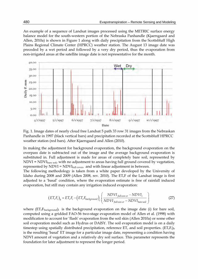
An example of a sequence of Landsat images processed using the METRIC surface energy balance model for the south-western portion of the Nebraska Panhandle (Kjaersgaard and Allen, 2010a) is shown in Figure 1 along with daily precipitation from the Scottsbluff High Plains Regional Climate Center (HPRCC) weather station. The August 13 image date was preceded by a wet period and followed by a very dry period, thus the evaporation from non-irrigated areas at the satellite image date is not representative for the month.

Fig. 1. Image dates of nearly cloud free Landsat 5 path 33 row 31 images from the Nebraskan Panhandle in 1997 (black vertical bars) and precipitation recorded at the Scottsbluff HPRCC weather station (red bars). After Kjaersgaard and Allen (2010).

In making the adjustment for background evaporation, the background evaporation on the overpass date is subtracted out of the image and the average background evaporation is substituted in. Full adjustment is made for areas of completely bare soil, represented by NDVI = NDVIbare soil, with no adjustment to areas having full ground covered by vegetation, represented by NDVI = NDVIfull cover, and with linear adjustment in between. The following methodology is taken from a white paper developed by the University of Idaho during 2008 and 2009 (Allen 2008, rev. 2010). The ETrF of the Landsat image is first adjusted to a ‘basal’ condition, where the evaporation estimate is free of rainfall induced evaporation, but still may contain any irrigation induced evaporation:

cov

cov

full er ir i r i r backgroundb i

full er baresoil

NDVI NDVIET F ET F ET F

NDVI NDVI

(27)

where (ETrFbackground)i is the background evaporation on the image date (i) for bare soil, computed using a gridded FAO-56 two-stage evaporation model of Allen et al. (1998) with modification to account for ‘flash’ evaporation from the soil skin (Allen 2010a) or some other soil evaporation model such as Hydrus or DAISY. The soil evaporation model is on a daily timestep using spatially distributed precipitation, reference ET, and soil properties. (ETrFi)b is the resulting ‘basal’ ET image for a particular image date, representing a condition having NDVI amount of vegetation and a relatively dry soil surface. This parameter represents the foundation for later adjustment to represent the longer period.


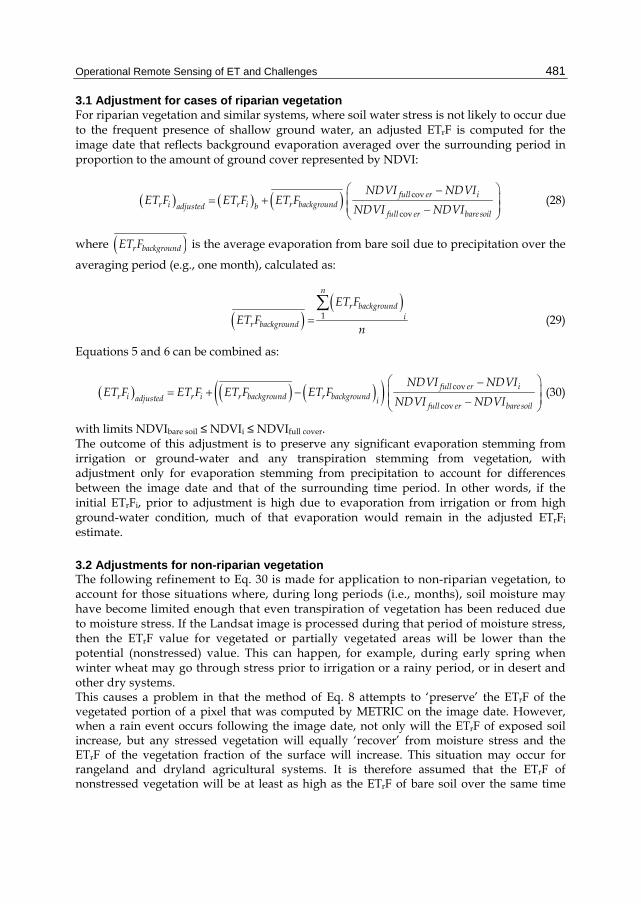
3.1 Adjustment for cases of riparian vegetation For riparian vegetation and similar systems, where soil water stress is not likely to occur due to the frequent presence of shallow ground water, an adjusted ETrF is computed for the image date that reflects background evaporation averaged over the surrounding period in proportion to the amount of ground cover represented by NDVI:

cov

cov

full er ir i r i r backgroundadjusted b

full er baresoil

NDVI NDVIET F ET F ET F

NDVI NDVI

(28)

where r backgroundET F is the average evaporation from bare soil due to precipitation over the

averaging period (e.g., one month), calculated as:

1

n

r backgroundi

r background

ET F

ET Fn

(29)

Equations 5 and 6 can be combined as:

cov

cov

full er ir i r i r background r backgroundadjusted i

full er bare soil

NDVI NDVIET F ET F ET F ET F

NDVI NDVI

(30)

with limits NDVIbare soil ≤ NDVIi ≤ NDVIfull cover. The outcome of this adjustment is to preserve any significant evaporation stemming from irrigation or ground-water and any transpiration stemming from vegetation, with adjustment only for evaporation stemming from precipitation to account for differences between the image date and that of the surrounding time period. In other words, if the initial ETrFi, prior to adjustment is high due to evaporation from irrigation or from high ground-water condition, much of that evaporation would remain in the adjusted ETrFi estimate.

3.2 Adjustments for non-riparian vegetation The following refinement to Eq. 30 is made for application to non-riparian vegetation, to account for those situations where, during long periods (i.e., months), soil moisture may have become limited enough that even transpiration of vegetation has been reduced due to moisture stress. If the Landsat image is processed during that period of moisture stress, then the ETrF value for vegetated or partially vegetated areas will be lower than the potential (nonstressed) value. This can happen, for example, during early spring when winter wheat may go through stress prior to irrigation or a rainy period, or in desert and other dry systems. This causes a problem in that the method of Eq. 8 attempts to ‘preserve’ the ETrF of the vegetated portion of a pixel that was computed by METRIC on the image date. However, when a rain event occurs following the image date, not only will the ETrF of exposed soil increase, but any stressed vegetation will equally ‘recover’ from moisture stress and the ETrF of the vegetation fraction of the surface will increase. This situation may occur for rangeland and dryland agricultural systems. It is therefore assumed that the ETrF of nonstressed vegetation will be at least as high as the ETrF of bare soil over the same time


period, since it should have equal access to shallow water. An exception would be if the vegetation were sufficiently stressed to not recover transpiration potential. However, this amount of stress should be evidenced by a reduced NDVI. A minimum limit is therefore

placed, using the background ETrF r backgroundET F for the period.

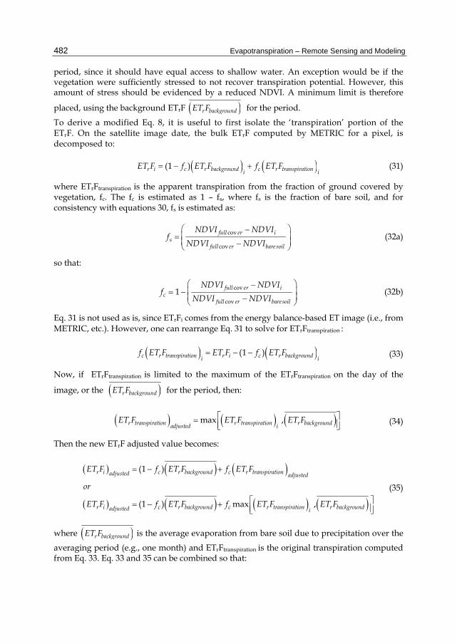
To derive a modified Eq. 8, it is useful to first isolate the ‘transpiration’ portion of the ETrF. On the satellite image date, the bulk ETrF computed by METRIC for a pixel, is decomposed to:

(1 )r i c r background c r transpirationi iET F f ET F f ET F (31)

where ETrFtranspiration is the apparent transpiration from the fraction of ground covered by vegetation, fc. The fc is estimated as 1 – fs, where fs is the fraction of bare soil, and for consistency with equations 30, fs is estimated as:

cov

cov

full er is

full er bare soil

NDVI NDVIf

NDVI NDVI

(32a)

so that:

cov

cov

1 full er ic

full er bare soil

NDVI NDVIf

NDVI NDVI

(32b)

Eq. 31 is not used as is, since ETrFi comes from the energy balance-based ET image (i.e., from METRIC, etc.). However, one can rearrange Eq. 31 to solve for ETrFtranspiration :

(1 )c r transpiration r i c r backgroundi if ET F ET F f ET F (33)

Now, if ETrFtranspiration is limited to the maximum of the ETrFtranspiration on the day of the

image, or the r backgroundET F for the period, then:

max ,r transpiration r transpiration r backgroundadjusted iET F ET F ET F (34)

Then the new ETrF adjusted value becomes:

(1 )

(1 ) max ,

r i c r background c r transpirationadjusted adjusted

r i c r background c r transpiration r backgroundadjusted i

ET F f ET F f ET F

or

ET F f ET F f ET F ET F

(35)

where r backgroundET F is the average evaporation from bare soil due to precipitation over the

averaging period (e.g., one month) and ETrFtranspiration is the original transpiration computed from Eq. 33. Eq. 33 and 35 can be combined so that:


(1 )

max (1 ) ,

r i c r backgroundadjusted

r i c r background c r backgroundi i

ET F f ET F

ET F f ET F f ET F

(36)

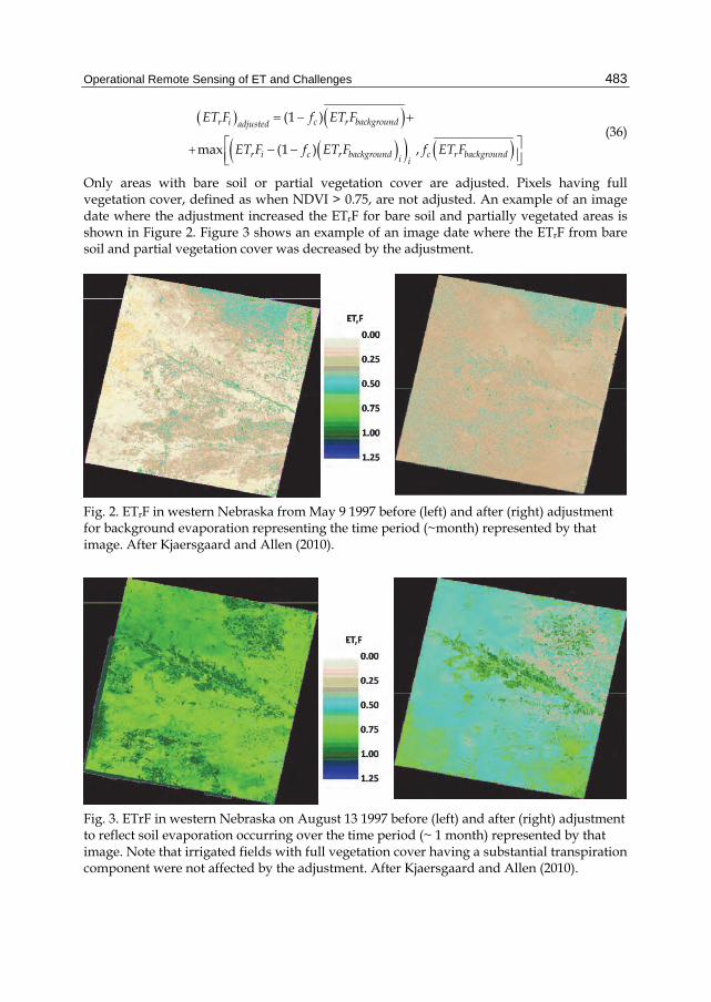
Only areas with bare soil or partial vegetation cover are adjusted. Pixels having full vegetation cover, defined as when NDVI > 0.75, are not adjusted. An example of an image date where the adjustment increased the ETrF for bare soil and partially vegetated areas is shown in Figure 2. Figure 3 shows an example of an image date where the ETrF from bare soil and partial vegetation cover was decreased by the adjustment.

Fig. 2. ETrF in western Nebraska from May 9 1997 before (left) and after (right) adjustment for background evaporation representing the time period (~month) represented by that image. After Kjaersgaard and Allen (2010).

Fig. 3. ETrF in western Nebraska on August 13 1997 before (left) and after (right) adjustment to reflect soil evaporation occurring over the time period (~ 1 month) represented by that image. Note that irrigated fields with full vegetation cover having a substantial transpiration component were not affected by the adjustment. After Kjaersgaard and Allen (2010).


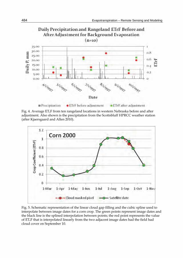
Fig. 4. Average ETrF from ten rangeland locations in western Nebraska before and after adjustment. Also shown is the precipitation from the Scottsbluff HPRCC weather station (after Kjaersgaard and Allen 2010).

Fig. 5. Schematic representation of the linear cloud gap filling and the cubic spline used to interpolate between image dates for a corn crop. The green points represent image dates and the black line is the splined interpolation between points; the red point represents the value of ETrF that is interpolated linearly from the two adjacent image dates had the field had cloud cover on September 10.


Average ETrF on image dates before and after adjustment for background evaporation is shown in Figure 4 from ten rangeland locations in western Nebraska. For some image dates, such as early and late in the season, the adjusted ETrF values are “wetter” than that represented by the original image. Similarly, for other images dates, such as in the middle of the growing season, the images were “drier”. The adjustment for one image in August reduced the estimated ET for the month of August by nearly 50%, which is considerable. It is noted, that the images no longer represent the ET from the satellite overpass dates after the adjustment for background evaporation. The images are merely an intermediate product that is used as the input into an interpolation procedure when producing ET estimates for monthly or longer time periods.

4. Dealing with clouded parts of images

Satellite images often have clouds in portions of the images. ETrF cannot be directly estimated for these areas using surface energy balance because cloud temperature masks surface temperature and cloud albedo masks surface albedo. Generally ETrF for clouded areas must be filled in before application of further integration processes so that those processes can be uniformly applied to an entire image. The alternative is to directly interpolate ETrF between adjacent (in time) image dates or to run some type of daily ET process model that is based on gridded weather data. In METRIC applications (Allen et al. 2007b), ETrF for clouded areas of images is usually filled in prior to interpolating ETrF for days between image dates (and multiplying by gridded ETr for each day to obtain daily ET images). A linear interpolation, as shown in Figure 5, is used to fill in ETrF for clouded portions of images rather than curvilinear interpolation that is used to interpolate ETrF between nonclouded image portions because some periods between cloud-free pixel locations can be as long as several months. Often, the change in crop vegetation amount and thus ETrF is uncertain during that period. Thus, the use of curvilinear interpolation can become speculative. Image processing code can be created to conduct the ‘filling’ of cloud masked portions of images. The code used with METRIC accommodates up to eight image dates and corresponding ETrF, with conditionals used to select the appropriate set of images to interpolate between, depending on the number of consecutive images that happen to be cloud masked for any specific location. Missing (clouded) ETrF for end-member images (those at the start or end of the growing season) must be estimated by extrapolation of the nearest (in time) image having valid ETrF, or alternatively, for end-member images, a ‘synthetic’ image can be created, based on daily soil water balance or other methods, to be used to substitute for cloud-masked areas. Often, the availability of images for early spring is limited due to clouds. In these cases, the ETrF values in the synthetic image are based on a soil-water balance–weather data model, such as the FAO-56 evaporation model or Hydrus or DAISY, applied over the month of April, for example, to provide an improved estimate of ETrF over the early season. The synthetic image(s) are strategically placed, date-wise, so that the cloud-filling process and the subsequent cubic spline process used to interpolate final ETrF has end-points early enough in the year to provide ETrF for all days of interest during the growing period. Examples of cloud masking for a METRIC application in western Nebraska are shown in Figure 6. Black portions within each image are the areas masked for clouds. ETrF for cloud


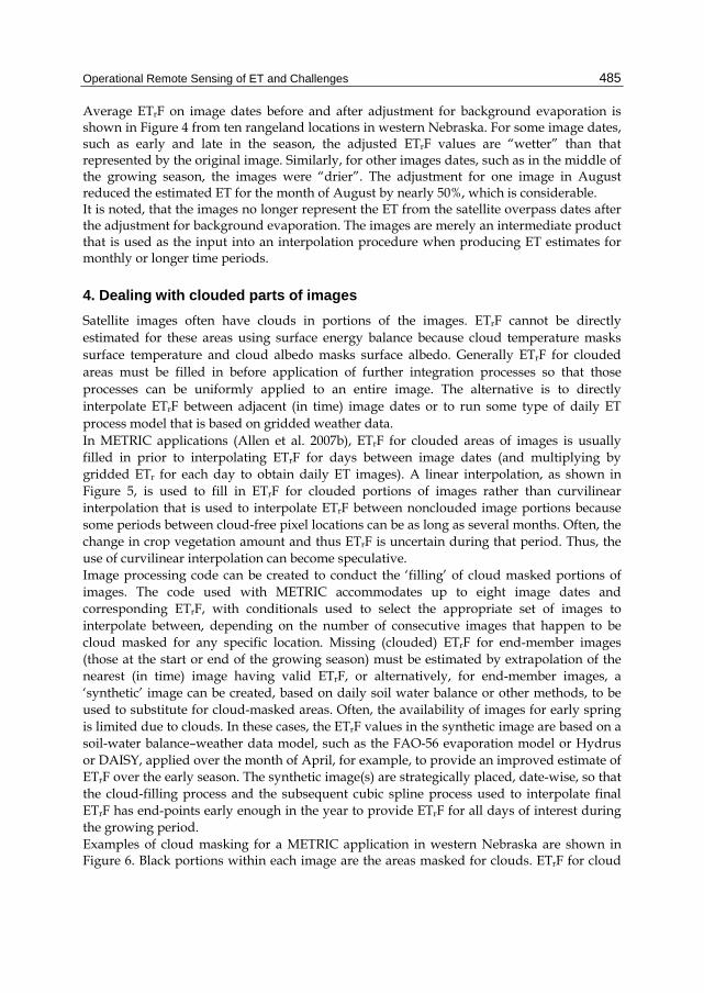
masked areas was filled in for individual Landsat dates prior to splining ETrF between images. The cloud mask gap filling and interpolation of ET between image dates entails interpolating the ETrF for the missing area from the previous and following images that have ETrF for that location.

Fig. 6. Maps of cloud masked ETrF from seven 1997 images dates. The geographical extent of the North Platte and South Platte Natural Resource Districts boundaries and principal cities is shown on the image in the top left corner (after Kjaersgaard and Allen 2010).

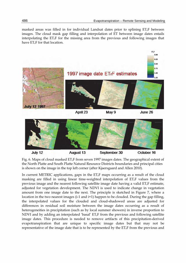
In current METRIC applications, gaps in the ETrF maps occurring as a result of the cloud masking are filled in using linear time-weighted interpolation of ETrF values from the previous image and the nearest following satellite image date having a valid ETrF estimate, adjusted for vegetation development. The NDVI is used to indicate change in vegetation amount from one image date to the next. The principle is sketched in Figure 7, where a location in the two nearest images (i-1 and i+1) happen to be clouded. During the gap filling, the interpolated values for the clouded and cloud-shadowed areas are adjusted for differences in residual soil moisture between the image dates occurring as a result of heterogeneities in precipitation (such as by local summer showers) in inverse proportion to NDVI and by adding an interpolated ‘basal’ ETrF from the previous and following satellite image dates. This procedure is needed to remove artifacts of this precipitation-derived evapotranspiration that are unique to specific image dates but that may not be representative of the image date that is to be represented by the ETrF from the previous and


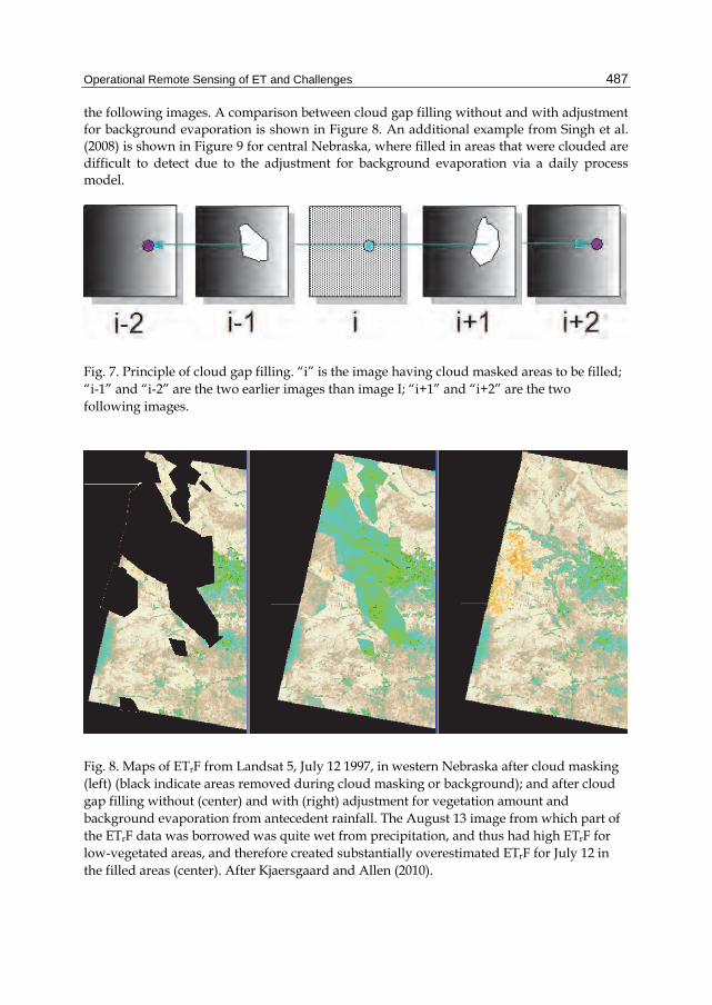
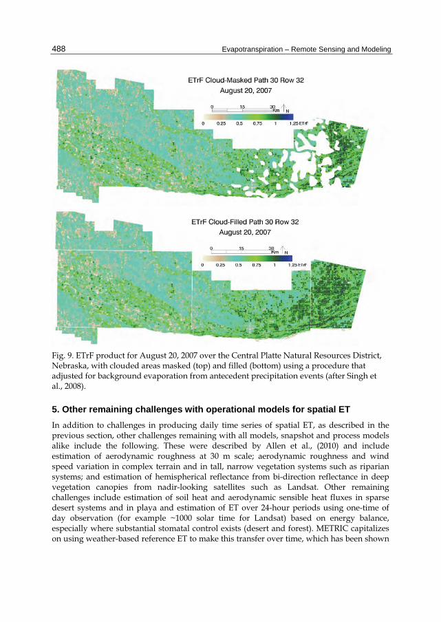
the following images. A comparison between cloud gap filling without and with adjustment for background evaporation is shown in Figure 8. An additional example from Singh et al. (2008) is shown in Figure 9 for central Nebraska, where filled in areas that were clouded are difficult to detect due to the adjustment for background evaporation via a daily process model.

Fig. 7. Principle of cloud gap filling. “i” is the image having cloud masked areas to be filled; “i-1” and “i-2” are the two earlier images than image I; “i+1” and “i+2” are the two following images.

Fig. 8. Maps of ETrF from Landsat 5, July 12 1997, in western Nebraska after cloud masking (left) (black indicate areas removed during cloud masking or background); and after cloud gap filling without (center) and with (right) adjustment for vegetation amount and background evaporation from antecedent rainfall. The August 13 image from which part of the ETrF data was borrowed was quite wet from precipitation, and thus had high ETrF for low-vegetated areas, and therefore created substantially overestimated ETrF for July 12 in the filled areas (center). After Kjaersgaard and Allen (2010).


Fig. 9. ETrF product for August 20, 2007 over the Central Platte Natural Resources District, Nebraska, with clouded areas masked (top) and filled (bottom) using a procedure that adjusted for background evaporation from antecedent precipitation events (after Singh et al., 2008).

5. Other remaining challenges with operational models for spatial ET

In addition to challenges in producing daily time series of spatial ET, as described in the previous section, other challenges remaining with all models, snapshot and process models alike include the following. These were described by Allen et al., (2010) and include estimation of aerodynamic roughness at 30 m scale; aerodynamic roughness and wind speed variation in complex terrain and in tall, narrow vegetation systems such as riparian systems; and estimation of hemispherical reflectance from bi-direction reflectance in deep vegetation canopies from nadir-looking satellites such as Landsat. Other remaining challenges include estimation of soil heat and aerodynamic sensible heat fluxes in sparse desert systems and in playa and estimation of ET over 24-hour periods using one-time of day observation (for example ~1000 solar time for Landsat) based on energy balance, especially where substantial stomatal control exists (desert and forest). METRIC capitalizes on using weather-based reference ET to make this transfer over time, which has been shown


to work well for irrigated crops, especially in advective environments (Allen et al. 2007a). However, the evaporative fraction, as used in early SEBAL (Bastiaanssen et al. 1998a) and other models may perform best for rainfed systems where, by definition, advection can not exist. Therefore, a mixture of ETrF and EF may be optimal, based on land-use class.

6. Conclusions

Satellite-based models for determining evapotranspiration (ET) are now routinely applied as part of water and water resources management operations of state and federal agencies. The very strong benefit of satellite-based models is the quantification of ET over large areas. Strengths and weaknesses of common EB models often dictate their use. The more widely used and operational remote sensing models tend to use a 'CIMEC' approach ("calibration using inverse modeling of extreme conditions") to calibrate around uncertainties and biases in satellite based energy balance components. Creating ‘maps’ of ET that are useful in management and in quantifying and managing water resources requires the computation of ET over monthly and longer periods such as growing seasons or annual periods. This requires accounting for increases in ET from precipitation events in between images. An approach for estimating the impacts on ET from wetting events in between images has been described. This method is empirical and can be improved in the future with more complex, surface conductance types of process models, such as used in Land surface models (LSM’s). Interpolation processes involve treatment of clouded areas of images, accounting for evaporation from wetting events occurring prior to or following overpass dates, and applying a grid of daily reference ET with the relative ET computed for an image, or a direct Penman-Monteith type of calculation. These approaches constitute a big step forward in computing seasonal ET over large areas with relatively high spatial (field-scale) definition, where impacts of intervening wetting events and cloud occurrence are addressed.

7. References

Abrahamsen, P. and S. Hansen . 2000. Daisy: an open soil-crop-atmosphere system model. Environmental Modelling and Software, 15(3):313-330.

Allen, R.G. 2008, rev. 2010. Procedures for adjusting METRIC-derived ETrF Images for Background Evaporation from Precipitation Events prior to Cloudfilling and Interpretation of ET between Image Dates. Internal memo., University of Idaho. 11 pages. Version 7, last revised April 2010.

Allen, R.G., 2010a. Modification to the FAO-56 Soil Surface Evaporation Algorithm to Account for Skin Evaporation during Small Precipitation Events. Memorandum prepared for the UI Remote Sensing Group, revised May 16, 2010, August 2010, 9 pages.

Allen, R.G. 2010b. Assessment of the probability of being able to produce Landsat resolution images of annual (or growing season) evapotranspiration in southern Idaho – and effect of the number of satellites. Memorandum prepared for the Landsat Science Team. 5 p.

Allen, R.G. and Wright, J.L. (1997). Translating Wind Measurements from Weather Stations to Agricultural Crops. J. Hydrologic Engineering, ASCE 2(1): 26-35.

Allen, R.G. and Trezza, R. (2011). New aerodynamic functions for application of METRIC in mountainous areas. Internal memo. University of Idaho, Kimberly, ID. 12 p.


Allen, R. G., Pereira, L., Raes, D., and Smith, M. 1998. Crop Evapotranspiration, Food and Agriculture Organization of the United Nations, Rome, It. ISBN 92-5-104219-5. 300 p.

Allen, R.G., W.B.M. Bastiaanssen, M. Tasumi, and A. Morse. 2001. Evapotranspiration on the watershed scale using the SEBAL model and LandSat Images. Paper Number 01-2224, ASAE, Annual International Meeting, Sacramento, California, July 30-August 1, 2001.

Allen, R.G., M.Tasumi, A.T. Morse, and R. Trezza. 2005. A Landsat-based Energy Balance and Evapotranspiration Model in Western US Water Rights Regulation and Planning. J. Irrigation and Drainage Systems. 19: 251-268.

Allen, R.G., M. Tasumi and R. Trezza. 2007a. Satellite-based energy balance for mapping evapotranspiration with internalized calibration (METRIC) – Model. ASCE J. Irrigation and Drainage Engineering 133(4):380-394.

Allen, R.G., M. Tasumi, A.T. Morse, R. Trezza, W. Kramber, I. Lorite and C.W. Robison. 2007b. Satellite-based energy balance for mapping evapotranspiration with internalized calibration (METRIC) – Applications. ASCE J. Irrigation and Drainage Engineering 133(4):395-406.

Allen,R.G., J. Kjaersgaard, R. Trezza, A. Oliveira, C. Robison, and I. Lorite-Torres. 2010. Refining components of a satellite based surface energy balance model to complex-land use systems. Proceedings of the Remote Sensing and Hydrology Symposium, Jackson Hole, Wyo, IAHS. Oct. 2010. 3 p.

Anderson, M.C., Kustas, W.P., Dulaney, W., Feng, G., Summer, D., 2010. Integration of Multi-Scale Thermal Satellite Imagery for Evaluation of Daily Evapotranspiration at the Sub-Field Scale. Remote Sensing and Hydrology Symposium 2010. Jackson Hole, Wyoming, USA. p. 62.

Arnold, J.G., J.R. Williams, R. Srinivasan, K.W. King and R.H. Griggs. 1994. SWAT--Soil and Water Assessment Tool--User Manual. Agricultural Research Service, Grassland, Soil and Water Research Lab, US Department of Agriculture.

ASCE – EWRI. (2005). The ASCE Standardized reference evapotranspiration equation. ASCE-EWRI Standardization of Reference Evapotranspiration Task Comm. Report, ASCE Bookstore, ISBN 078440805, Stock Number 40805, 216 pages.

Bastiaanssen, W.G.M., M. Menenti, R.A. Feddes, and A.A. M. Holtslag. 1998a. A remote sensing surface energy balance algortithm for land (SEBAL). Part 1: Formulation. J. of Hydrology 198-212.

Bastiaanssen, W.G.M., H. Pelgrum, J. Wang, Y. Ma, J.F. Moreno, G.J. Roerink, R.A. Roebeling, and T. van der Wal. 1998b. A remote sensing surface energy balance algortithm for land (SEBAL). Part 2: Validation. J. of Hydrology 212-213: 213-229.

Bastiaanssen , W.G.M., E.J.M. Noordman , H. Pelgrum, G. Davids, B.P. Thoreson and R.G. Allen. 2005. SEBAL model with remotely sensed data to improve water resources management under actual field conditions. J. Irrig. Drain. Engrg, ASCE 131(1): 85-93.

Brutsaert, W. 1982. Evaporation into the atmosphere. Reidel, Dordrecht, The Netherlands. Brutsaert, W., A.Y. Hsu, and T.J. Schmugge. 1993. Parameterization of surface heat fluxes

above a forest with satellite thermal sensing and boundary layer soundings. J. Appl. Met. 32: 909-917.


Campbell, G.S. and J.M. Norman. 1998. An introduction to environmental biophysics. Sec. Edition. Springer, New York.

Cleugh, H.A., R. Leuning, Q. Mu and S.W. Running. 2007. Regional evaporation estimates from flux tower and MODIS satellite data. Remote Sens. Environ. 106:285-304.

Colaizzi, P.D., S. R. Evett, T. A. Howell, J. A. Tolk. 2006. Comparison of Five Models to Scale Daily Evapotranspiration from One-Time-of-Day Measurements. Trans. ASABE. 49(5):1409-1417.

Farah, H.O. 2001. Estimation of regional evaporation under different weather conditions from satellite and meteorological data. A case study in the Naivasha Basin, Kenya. Doctoral Thesis Wageningen University and ITC.

Franks, S.W. and K.J. Beven. 1997. Estimation of evapotranspiration at the landscape scale: a fuzzy disaggregation approach. Water Resour. Res. 33:2929-2938.

Gao, F., Masek, J., Schwaller, M., Hall, F., 2006. On the Blending of the Landsat and Modis Surface Reflectance: Predicting Daily Landsat Surface Reflectance. IEEE Trans on Geosci. and Remote Sens. 44, 2207-2218.

Gowda, P.H., J.L. Chávez, P.D. Colaizzi, S.R. Evett, T.A. Howell, and J.A. Tolk. 2008. ET mapping for agricultural water management: present status and challenges. Irrig. Sci. 26:223-237

Groeneveld, D.P., W.J. baugh, J.S. Sanderson and D.J. Cooper. 2007. Annual groundwater evapotranspiration mapped from single satellite scenes. J. Hydrol. 344:146-156.

Hall, F.G., K.F. Huemmrich, S.J. Goetz, P.J. Sellers, and J.E. Nickeson. 1992. Satellite remote sensing of the surface energy balance: success, failures and unresolved issues in FIFE. J. Geophys. Res. 97(D17):19061-19090.

Hook, S. and A.J. Prata. 2001. Land surface termpature measured by ASTER-First results. Geophys. Res. Abs., 26th Gen. Assemb. 3:71.

Jensen, M.E., Burman, R.D. and Allen, R.G. (eds.) (1990). Evapotranspiration and Irrigation Water Requirements, ASCE Manuals and Reports on Engineering Practice No. 70. ISBN 0-87262-763-2, 332 p. ASCE, Reston, VA.

Kalma, J.D. and D.L.B. Jupp. 1990. Estimating evaporation from pasture using infrared thermography: evaluation of a one-layer resistance model. Agr. and Forest Met. 51:223-246.

Kalma, J.D., T.R. McVicar, and M.F. McCabe. 2008. Estimating land surface evaporation: a review of methods using remotely sensed surface temperature data. Surv. Geophys 29:421-469.

Kjaersagaard, J. and R.G. Allen. 2010. Remote Sensing Technology to Produce Consumptive Water Use Maps for the Nebraska Panhandle. Final completion report submitted to the University of Nebraska. 60 pages.

Kustas, W. P., and J. M. Norman. 1996. Use of remote sensing for evapotranspiration monitoring over land surfaces. Hydrol. Sci. J. 41(4): 495-516.

Kustas, W. P., Moran, M. S., Humes, K. S., Stannard, D. I., Pinter, J., Hipps, L., and Goodrich, D. C. 1994. Surface energy balance estimates at local and regional scales using optical remote sensing from an aircraft platform and atmospheric data collected over semiarid rangelands. Water Resources Research, 30(5): 1241-1259.

Oke, T.R, (1987). Boundary Layer Climates. 2nd Ed., Methuen, London, 435 pp, ISBN 0-415-04319-0.


Paulson, C.A. (1970). The mathematical representation of wind speed and temperature profiles in the unstable atmospheric surface layer. Appl. Meteorol. 9:857-861.

Qualls, R., and Brutsaert, W. (1996). “Effect of vegetation density on the parameterization of scalar roughness to estimate spatially distributed sensible heat fluxes.” Water Resources Research, 32(3): 645-652.

Qualls, R., and Hopson, T. (1998). “Combined use of vegetation density, friction velocity, and solar elevation to parameterize the scalar roughness for sensible heat.” J. Atmospheric Sciences, 55: 1198-1208.

Romero, M.G. (2004) Daily evapotranspiration estimation by means of evaporative fraction and reference ET fraction. Ph.D. Diss., Utah State Univ., Logan, Utah.

Rosema, A. 1990. Comparison of meteosat-based rainfall and evapotranspiration mapping of Sahel region. Rem. Sens. Env. 46: 27-44.

Šimůnek, J., M.T. van Genuchten, and M. Šejna. 2008. Development and applications of the HYDRUS and STANMOD software packages and related codes. Vadose Zone J. 7:587-600.

Singh, R.K., A. Irmak, S. Irmak and D.L. Martin. 2008. Application of SEBAL Model for Mapping Evapotranspiration and Estimating Surface Energy Fluxes in South-Central Nebraska. J. Irrigation and Drainage Engineering 134(3):273-285.

Su, Z. 2002. The surface energy balance system (SEBS) for estimation of turbulent fluxes. Hydrol. Earth Systems Sci. 6(1): 85-99.

Tasumi, M., R. G. Allen, R. Trezza, J. L. Wright. 2005. Satellite-based energy balance to assess within-population variance of crop coefficient curves, J. Irrig. and Drain. Engrg, ASCE 131(1): 94-109.

Van Dam, J.C., 2000. Field-scale water flow and solute transport: SWAP model concepts, parameter estimation and case studies. Proefschrift Wageningen Universiteit.

Wang, J., W.G.M Bastiaanssen, Y. Ma, and H. Pelgrum. 1998. Aggregation of land surface parameters in the oasis-desert systems of Northwest China. Hydr. Processes 12:2133-2147.

Webb, E.K. (1970). Profile relationships: the log-linear range, and extension to strong stability. Quart. J. Roy. Meteorol. Soc. 96:67-90.

Wright, J.L. (1982) New Evapotranspiration Crop Coefficients. J. of Irrig. and Drain. Div. (ASCE), 108:57-74.

Documents

Operational Remote Sensing of ET and Challenges Operational Remote Sensing of ET and Challenges Ayse Irmak1, Richard G. Allen2, Jeppe Kjaersgaard2, Justin Huntington3, Baburao Kamble4,