Embed Size (px)
Citation preview
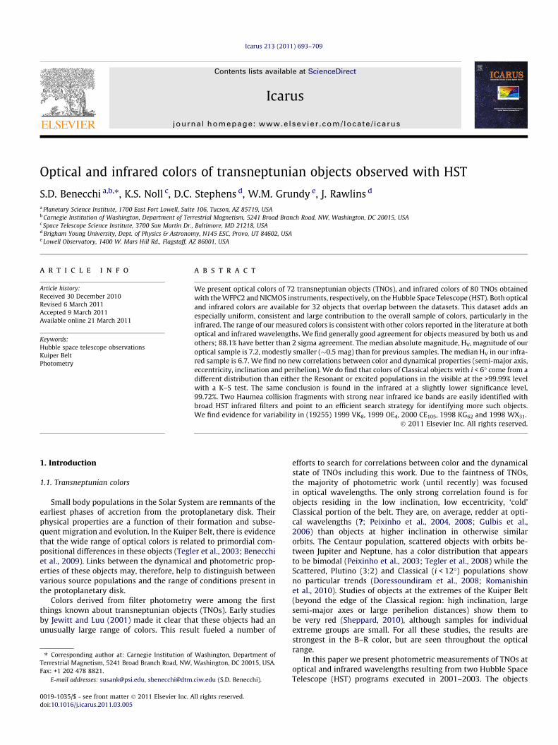
Icarus 213 (2011) 693–709
Contents lists available at ScienceDirect
Icarus
journal homepage: www.elsevier .com/locate / icarus
Optical and infrared colors of transneptunian objects observed with HST
S.D. Benecchi a,b,⇑, K.S. Noll c, D.C. Stephens d, W.M. Grundy e, J. Rawlins d
a Planetary Science Institute, 1700 East Fort Lowell, Suite 106, Tucson, AZ 85719, USAb Carnegie Institution of Washington, Department of Terrestrial Magnetism, 5241 Broad Branch Road, NW, Washington, DC 20015, USAc Space Telescope Science Institute, 3700 San Martin Dr., Baltimore, MD 21218, USAd Brigham Young University, Dept. of Physics & Astronomy, N145 ESC, Provo, UT 84602, USAe Lowell Observatory, 1400 W. Mars Hill Rd., Flagstaff, AZ 86001, USA
a r t i c l e i n f o
Article history:Received 30 December 2010Revised 6 March 2011Accepted 9 March 2011Available online 21 March 2011
Keywords:Hubble space telescope observationsKuiper BeltPhotometry
0019-1035/$ - see front matter � 2011 Elsevier Inc. Adoi:10.1016/j.icarus.2011.03.005
⇑ Corresponding author at: Carnegie Institution ofTerrestrial Magnetism, 5241 Broad Branch Road, NW,Fax: +1 202 478 8821.
E-mail addresses: [email protected], sbenecchi@dtm
a b s t r a c t
We present optical colors of 72 transneptunian objects (TNOs), and infrared colors of 80 TNOs obtainedwith the WFPC2 and NICMOS instruments, respectively, on the Hubble Space Telescope (HST). Both opticaland infrared colors are available for 32 objects that overlap between the datasets. This dataset adds anespecially uniform, consistent and large contribution to the overall sample of colors, particularly in theinfrared. The range of our measured colors is consistent with other colors reported in the literature at bothoptical and infrared wavelengths. We find generally good agreement for objects measured by both us andothers; 88.1% have better than 2 sigma agreement. The median absolute magnitude, HV, magnitude of ouroptical sample is 7.2, modestly smaller (�0.5 mag) than for previous samples. The median HV in our infra-red sample is 6.7. We find no new correlations between color and dynamical properties (semi-major axis,eccentricity, inclination and perihelion). We do find that colors of Classical objects with i < 6� come from adifferent distribution than either the Resonant or excited populations in the visible at the >99.99% levelwith a K–S test. The same conclusion is found in the infrared at a slightly lower significance level,99.72%. Two Haumea collision fragments with strong near infrared ice bands are easily identified withbroad HST infrared filters and point to an efficient search strategy for identifying more such objects.We find evidence for variability in (19255) 1999 VK8, 1999 OE4, 2000 CE105, 1998 KG62 and 1998 WX31.
� 2011 Elsevier Inc. All rights reserved.
1. Introduction
1.1. Transneptunian colors
Small body populations in the Solar System are remnants of theearliest phases of accretion from the protoplanetary disk. Theirphysical properties are a function of their formation and subse-quent migration and evolution. In the Kuiper Belt, there is evidencethat the wide range of optical colors is related to primordial com-positional differences in these objects (Tegler et al., 2003; Benecchiet al., 2009). Links between the dynamical and photometric prop-erties of these objects may, therefore, help to distinguish betweenvarious source populations and the range of conditions present inthe protoplanetary disk.
Colors derived from filter photometry were among the firstthings known about transneptunian objects (TNOs). Early studiesby Jewitt and Luu (2001) made it clear that these objects had anunusually large range of colors. This result fueled a number of
ll rights reserved.
Washington, Department ofWashington, DC 20015, USA.
.ciw.edu (S.D. Benecchi).
efforts to search for correlations between color and the dynamicalstate of TNOs including this work. Due to the faintness of TNOs,the majority of photometric work (until recently) was focusedin optical wavelengths. The only strong correlation found is forobjects residing in the low inclination, low eccentricity, ‘cold’Classical portion of the belt. They are, on average, redder at opti-cal wavelengths (?; Peixinho et al., 2004, 2008; Gulbis et al.,2006) than objects at higher inclination in otherwise similarorbits. The Centaur population, scattered objects with orbits be-tween Jupiter and Neptune, has a color distribution that appearsto be bimodal (Peixinho et al., 2003; Tegler et al., 2008) while theScattered, Plutino (3:2) and Classical (i < 12�) populations showno particular trends (Doressoundiram et al., 2008; Romanishinet al., 2010). Studies of objects at the extremes of the Kuiper Belt(beyond the edge of the Classical region: high inclination, largesemi-major axes or large perihelion distances) show them tobe very red (Sheppard, 2010), although samples for individualextreme groups are small. For all these studies, the results arestrongest in the B–R color, but are seen throughout the opticalrange.
In this paper we present photometric measurements of TNOs atoptical and infrared wavelengths resulting from two Hubble SpaceTelescope (HST) programs executed in 2001–2003. The objects
1 A manufacturing defect in the WFPC2 CCD chip such that every 34th row isapproximately 3% narrower than all others. It induces errors in the photometry at the0.01–0.2 magnitude level if not corrected for following the methodology provided byAnderson and King (1999).
694 S.D. Benecchi et al. / Icarus 213 (2011) 693–709
observed were a subset of the full target list included as potentialtargets for these two ‘‘snapshot’’ programs. Potential targets wereselected based on predicted positional uncertainty and expectedtarget brightness.
1.2. Nomenclature
In this paper we adopt a modified dynamical classificationscheme using information available online (http://www.boulder.swri.edu/�buie/kbo/astrom/) or in the literature: Elliot et al.(2005, DES) and Gladman et al. (2008, GMV). We sort objects intoone of three possible categories: Resonant, Cold, or Hot. Resonantobjects are defined identically in the classification schemes of bothDES and GMV, they include any object in a mean motion resonancewith Neptune. Our Cold group includes Classicals with i 6 6�, an-other area of agreement between DES and GMV. Our Hot groupingincludes objects defined as Classicals with i > 6�, Scattered/Scatter-ing, Detached, and Centaurs. The definitions of these subgroups arewhere the DES and GMV differ. However, by grouping these objectstogether into a ‘‘Hot’’ category, the two classifications are again inagreement. There is abundant physical evidence for separating lowinclination Classicals as a distinct group including their color, asnoted above, their high concentration of binaries (Noll et al.,2008) and their high albedos (Brucker et al., 2009). According togiant planet migration models (e.g. the Nice model (Morbidelliet al., 2005; Levison et al., 2008; Tsiganis et al., 2005; Gomeset al., 2005)), much of the rest of the transneptunian populationmay be a mix of planetesimals scattered from a broad region ofthe protoplanetary nebula. There is no current unambiguous phys-ical evidence of distinct subpopulations to contradict this view. In-deed, it might well make sense to consider Resonant objects as partof the Hot population as well, although we retain this distinctionhere. About half our sample are Cold objects, with one quarter ofthe sample each in the Resonant and Hot groupings. We do notmeasure enough objects in any single Resonant population to war-rant dividing the objects farther. Likewise, we only measure a fewCentaurs so we are unable to separate out this population for addi-tional study.
2. Observations
In this paper we report observations associated with two differ-ent programs executed in HST Cycles 10 (June 2001–July 2002) and11 (August 2002–June 2003).
The first program, proposal 9060, observed 72 TNOs using theWide Field Planetary Camera 2 (WFPC2) in three broad filters:F555W (0.5442 lm) � V, F675W (0.6717 lm) � R, and F814W(0.7996 lm) � I. Objects were placed on the Wide Field Camera 3detector which has a pixel scale of 0.1 arcsec/pixel. The objectswere selected based on their small orbital uncertainties (630 arc-sec), without respect to dynamical classification, and had expectedV magnitudes between 22 and 24. Objects predicted to be brighterthan mV = 23.5 followed the observing sequence: 1 � 160 s inF555W, 2 � 160 s in F675W, 2 � 160 s in F814W, 1 � 160 s inF555W. For fainter objects, the F675W measurement was excludedand the exposure time was increased to 260 s for the other filters.The second program, proposal 9386, observed 80 TNOs using theNear Infrared Camera and Multi-Object Spectrometer (NICMOS),in two filters: F110W (1.1 lm) � J and F160W (1.6 lm) � H. Theobserving sequence was: 1 � 256 s in F110W, 2 � 512 s inF160W, 1 � 256 s in F110W. Objects were observed with theNIC2 camera which has a pixel scale 0.075 arcsec/pixel.
Observations in the WFPC2 program were not dithered. Obser-vations with Nicmos were dithered to mitigate the impact of hotpixels and other fixed pattern noise. The observations were brack-eted by the F555W filter in the optical, and the F110W filter in the
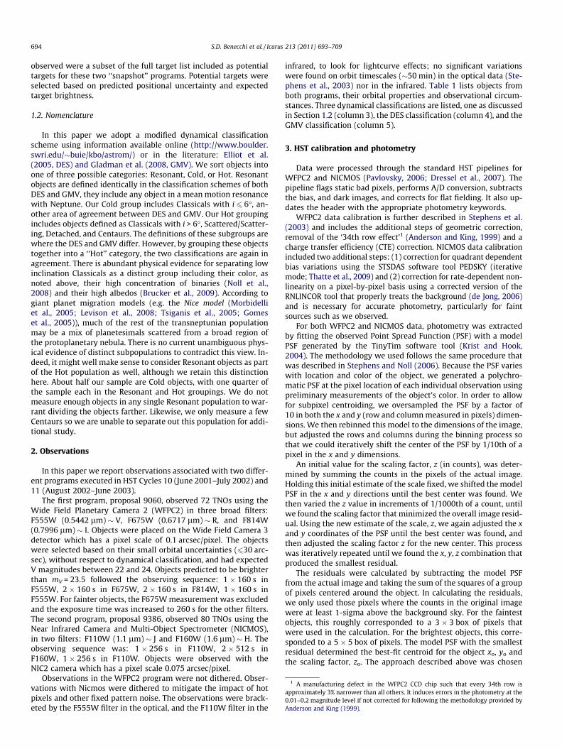
infrared, to look for lightcurve effects; no significant variationswere found on orbit timescales (�50 min) in the optical data (Ste-phens et al., 2003) nor in the infrared. Table 1 lists objects fromboth programs, their orbital properties and observational circum-stances. Three dynamical classifications are listed, one as discussedin Section 1.2 (column 3), the DES classification (column 4), and theGMV classification (column 5).
3. HST calibration and photometry
Data were processed through the standard HST pipelines forWFPC2 and NICMOS (Pavlovsky, 2006; Dressel et al., 2007). Thepipeline flags static bad pixels, performs A/D conversion, subtractsthe bias, and dark images, and corrects for flat fielding. It also up-dates the header with the appropriate photometry keywords.
WFPC2 data calibration is further described in Stephens et al.(2003) and includes the additional steps of geometric correction,removal of the ‘34th row effect’1 (Anderson and King, 1999) and acharge transfer efficiency (CTE) correction. NICMOS data calibrationincluded two additional steps: (1) correction for quadrant dependentbias variations using the STSDAS software tool PEDSKY (iterativemode; Thatte et al., 2009) and (2) correction for rate-dependent non-linearity on a pixel-by-pixel basis using a corrected version of theRNLINCOR tool that properly treats the background (de Jong, 2006)and is necessary for accurate photometry, particularly for faintsources such as we observed.
For both WFPC2 and NICMOS data, photometry was extractedby fitting the observed Point Spread Function (PSF) with a modelPSF generated by the TinyTim software tool (Krist and Hook,2004). The methodology we used follows the same procedure thatwas described in Stephens and Noll (2006). Because the PSF varieswith location and color of the object, we generated a polychro-matic PSF at the pixel location of each individual observation usingpreliminary measurements of the object’s color. In order to allowfor subpixel centroiding, we oversampled the PSF by a factor of10 in both the x and y (row and column measured in pixels) dimen-sions. We then rebinned this model to the dimensions of the image,but adjusted the rows and columns during the binning process sothat we could iteratively shift the center of the PSF by 1/10th of apixel in the x and y dimensions.
An initial value for the scaling factor, z (in counts), was deter-mined by summing the counts in the pixels of the actual image.Holding this initial estimate of the scale fixed, we shifted the modelPSF in the x and y directions until the best center was found. Wethen varied the z value in increments of 1/1000th of a count, untilwe found the scaling factor that minimized the overall image resid-ual. Using the new estimate of the scale, z, we again adjusted the xand y coordinates of the PSF until the best center was found, andthen adjusted the scaling factor z for the new center. This processwas iteratively repeated until we found the x, y, z combination thatproduced the smallest residual.
The residuals were calculated by subtracting the model PSFfrom the actual image and taking the sum of the squares of a groupof pixels centered around the object. In calculating the residuals,we only used those pixels where the counts in the original imagewere at least 1-sigma above the background sky. For the faintestobjects, this roughly corresponded to a 3 � 3 box of pixels thatwere used in the calculation. For the brightest objects, this corre-sponded to a 5 � 5 box of pixels. The model PSF with the smallestresidual determined the best-fit centroid for the object xo, yo andthe scaling factor, zo. The approach described above was chosen
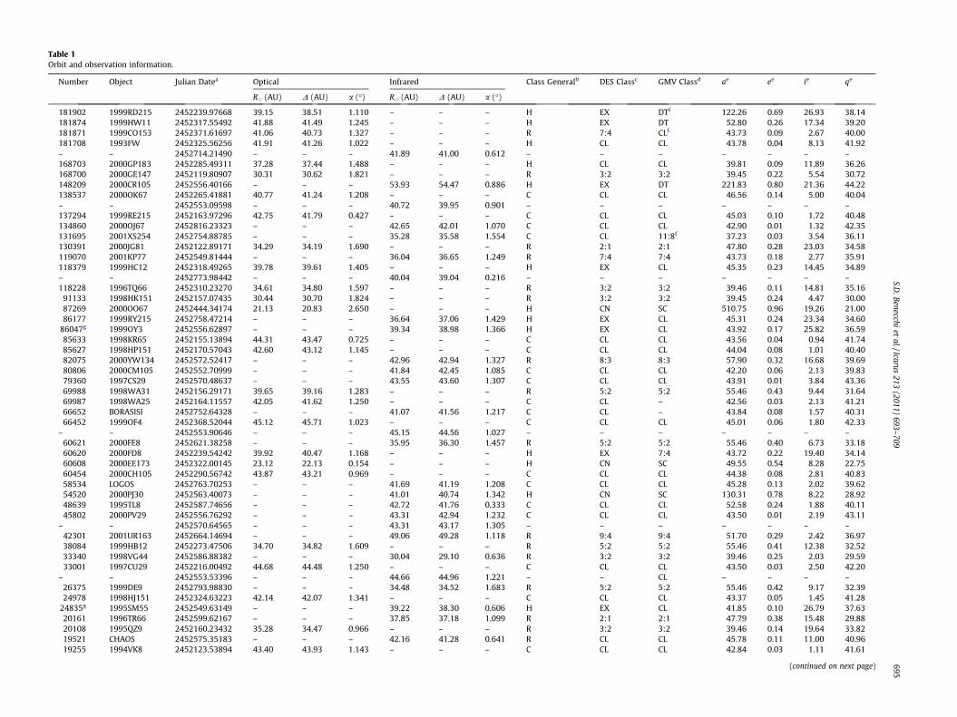
Table 1Orbit and observation information.
Number Object Julian Datea Optical Infrared Class Generalb DES Classc GMV Classd ae ee ie qe
R� (AU) D (AU) a (�) R� (AU) D (AU) a (�)
181902 1999RD215 2452239.97668 39.15 38.51 1.110 – – – H EX DTf 122.26 0.69 26.93 38.14181874 1999HW11 2452317.55492 41.88 41.49 1.245 – – – H EX DT 52.80 0.26 17.34 39.20181871 1999CO153 2452371.61697 41.06 40.73 1.327 – – – R 7:4 CLf 43.73 0.09 2.67 40.00181708 1993FW 2452325.56256 41.91 41.26 1.022 – – – H CL CL 43.78 0.04 8.13 41.92– – 2452714.21490 – – – 41.89 41.00 0.612 – – – – – – –168703 2000GP183 2452285.49311 37.28 37.44 1.488 – – – H CL CL 39.81 0.09 11.89 36.26168700 2000GE147 2452119.80907 30.31 30.62 1.821 – – – R 3:2 3:2 39.45 0.22 5.54 30.72148209 2000CR105 2452556.40166 – – – 53.93 54.47 0.886 H EX DT 221.83 0.80 21.36 44.22138537 2000OK67 2452265.41881 40.77 41.24 1.208 – – – C CL CL 46.56 0.14 5.00 40.04– – 2452553.09598 – – – 40.72 39.95 0.901 – – – – – – –137294 1999RE215 2452163.97296 42.75 41.79 0.427 – – – C CL CL 45.03 0.10 1.72 40.48134860 2000OJ67 2452816.23323 – – – 42.65 42.01 1.070 C CL CL 42.90 0.01 1.32 42.35131695 2001XS254 2452754.88785 – – – 35.28 35.58 1.554 C CL 11:8f 37.23 0.03 3.54 36.11130391 2000JG81 2452122.89171 34.29 34.19 1.690 – – – R 2:1 2:1 47.80 0.28 23.03 34.58119070 2001KP77 2452549.81444 – – – 36.04 36.65 1.249 R 7:4 7:4 43.73 0.18 2.77 35.91118379 1999HC12 2452318.49265 39.78 39.61 1.405 – – – H EX CL 45.35 0.23 14.45 34.89– – 2452773.98442 – – – 40.04 39.04 0.216 – – – – – – –118228 1996TQ66 2452310.23270 34.61 34.80 1.597 – – – R 3:2 3:2 39.46 0.11 14.81 35.16
91133 1998HK151 2452157.07435 30.44 30.70 1.824 – – – R 3:2 3:2 39.45 0.24 4.47 30.0087269 2000OO67 2452444.34174 21.13 20.83 2.650 – – – H CN SC 510.75 0.96 19.26 21.0086177 1999RY215 2452758.47214 – – – 36.64 37.06 1.429 H EX CL 45.31 0.24 23.34 34.60
86047g 1999OY3 2452556.62897 – – – 39.34 38.98 1.366 H EX CL 43.92 0.17 25.82 36.5985633 1998KR65 2452155.13894 44.31 43.47 0.725 – – – C CL CL 43.56 0.04 0.94 41.7485627 1998HP151 2452170.57043 42.60 43.12 1.145 – – – C CL CL 44.04 0.08 1.01 40.4082075 2000YW134 2452572.52417 – – – 42.96 42.94 1.327 R 8:3 8:3 57.90 0.32 16.68 39.6980806 2000CM105 2452552.70999 – – – 41.84 42.45 1.085 C CL CL 42.20 0.06 2.13 39.8379360 1997CS29 2452570.48637 – – – 43.55 43.60 1.307 C CL CL 43.91 0.01 3.84 43.3669988 1998WA31 2452156.29171 39.65 39.16 1.283 – – – R 5:2 5:2 55.46 0.43 9.44 31.6469987 1998WA25 2452164.11557 42.05 41.62 1.250 – – – C CL – 42.56 0.03 2.13 41.2166652 BORASISI 2452752.64328 – – – 41.07 41.56 1.217 C CL – 43.84 0.08 1.57 40.3166452 1999OF4 2452368.52044 45.12 45.71 1.023 – – – C CL CL 45.01 0.06 1.80 42.33
– – 2452553.90646 – – – 45.15 44.56 1.027 – – – – – – –60621 2000FE8 2452621.38258 – – – 35.95 36.30 1.457 R 5:2 5:2 55.46 0.40 6.73 33.1860620 2000FD8 2452239.54242 39.92 40.47 1.168 – – – H EX 7:4 43.72 0.22 19.40 34.1460608 2000EE173 2452322.00145 23.12 22.13 0.154 – – – H CN SC 49.55 0.54 8.28 22.7560454 2000CH105 2452290.56742 43.87 43.21 0.969 – – – C CL CL 44.38 0.08 2.81 40.8358534 LOGOS 2452763.70253 – – – 41.69 41.19 1.208 C CL CL 45.28 0.13 2.02 39.6254520 2000PJ30 2452563.40073 – – – 41.01 40.74 1.342 H CN SC 130.31 0.78 8.22 28.9248639 1995TL8 2452587.74656 – – – 42.72 41.76 0.333 C CL CL 52.58 0.24 1.88 40.1145802 2000PV29 2452556.76292 – – – 43.31 42.94 1.232 C CL CL 43.50 0.01 2.19 43.11
– – 2452570.64565 – – – 43.31 43.17 1.305 – – – – – – –42301 2001UR163 2452664.14694 – – – 49.06 49.28 1.118 R 9:4 9:4 51.70 0.29 2.42 36.9738084 1999HB12 2452273.47506 34.70 34.82 1.609 – – – R 5:2 5:2 55.46 0.41 12.38 32.5233340 1998VG44 2452586.88382 – – – 30.04 29.10 0.636 R 3:2 3:2 39.46 0.25 2.03 29.5933001 1997CU29 2452216.00492 44.68 44.48 1.250 – – – C CL CL 43.50 0.03 2.50 42.20
– – 2452553.53396 – – – 44.66 44.96 1.221 – – CL – – – –26375 1999DE9 2452793.98830 – – – 34.48 34.52 1.683 R 5:2 5:2 55.46 0.42 9.17 32.3924978 1998HJ151 2452324.63223 42.14 42.07 1.341 – – – C CL CL 43.37 0.05 1.45 41.28
24835g 1995SM55 2452549.63149 – – – 39.22 38.30 0.606 H EX CL 41.85 0.10 26.79 37.6320161 1996TR66 2452599.62167 – – – 37.85 37.18 1.099 R 2:1 2:1 47.79 0.38 15.48 29.8820108 1995QZ9 2452160.23432 35.28 34.47 0.966 – – – R 3:2 3:2 39.46 0.14 19.64 33.8219521 CHAOS 2452575.35183 – – – 42.16 41.28 0.641 R CL CL 45.78 0.11 11.00 40.9619255 1994VK8 2452123.53894 43.40 43.93 1.143 – – – C CL CL 42.84 0.03 1.11 41.61
(continued on next page)
S.D.Benecchi
etal./Icarus
213(2011)
693–709
695
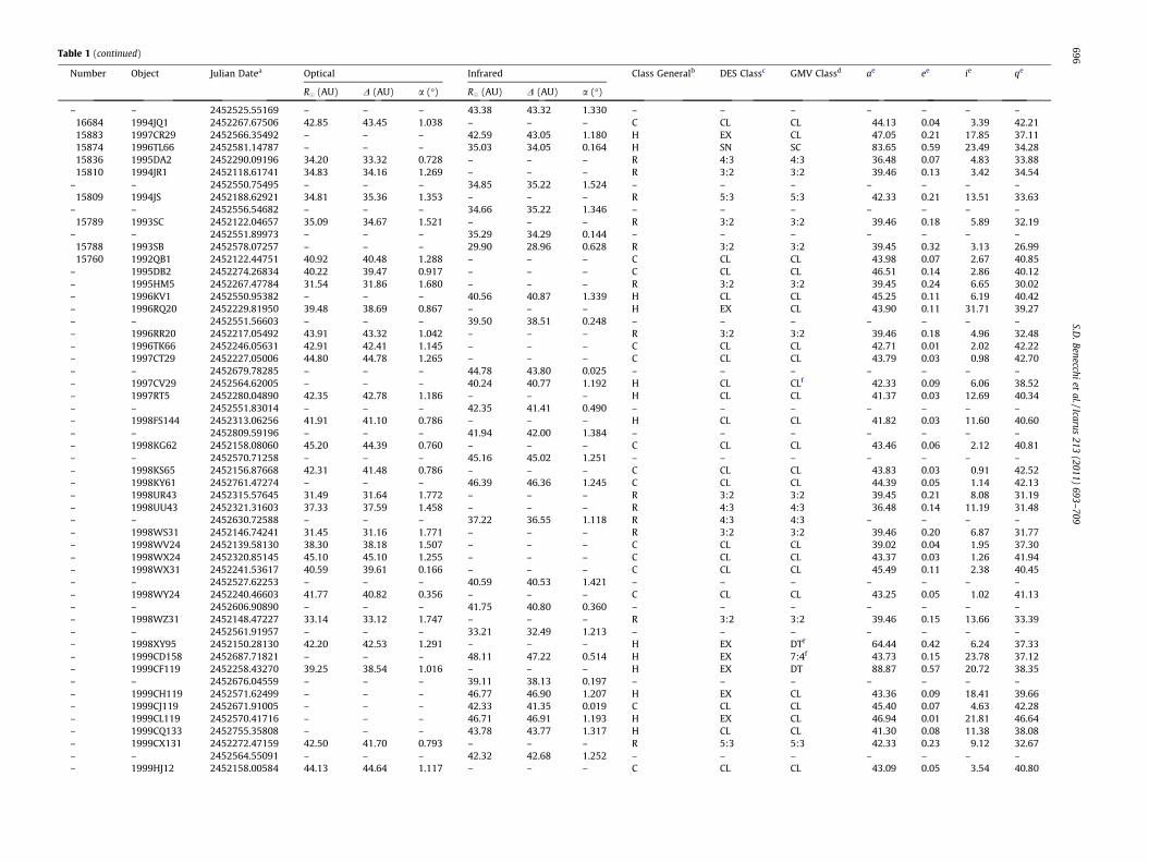
Table 1 (continued)
Number Object Julian Datea Optical Infrared Class Generalb DES Classc GMV Classd ae ee ie qe
R� (AU) D (AU) a (�) R� (AU) D (AU) a (�)
– – 2452525.55169 – – – 43.38 43.32 1.330 – – – – – – –16684 1994JQ1 2452267.67506 42.85 43.45 1.038 – – – C CL CL 44.13 0.04 3.39 42.2115883 1997CR29 2452566.35492 – – – 42.59 43.05 1.180 H EX CL 47.05 0.21 17.85 37.1115874 1996TL66 2452581.14787 – – – 35.03 34.05 0.164 H SN SC 83.65 0.59 23.49 34.2815836 1995DA2 2452290.09196 34.20 33.32 0.728 – – – R 4:3 4:3 36.48 0.07 4.83 33.8815810 1994JR1 2452118.61741 34.83 34.16 1.269 – – – R 3:2 3:2 39.46 0.13 3.42 34.54
– – 2452550.75495 – – – 34.85 35.22 1.524 – – – – – – –15809 1994JS 2452188.62921 34.81 35.36 1.353 – – – R 5:3 5:3 42.33 0.21 13.51 33.63
– – 2452556.54682 – – – 34.66 35.22 1.346 – – – – – – –15789 1993SC 2452122.04657 35.09 34.67 1.521 – – – R 3:2 3:2 39.46 0.18 5.89 32.19
– – 2452551.89973 – – – 35.29 34.29 0.144 – – – – – – –15788 1993SB 2452578.07257 – – – 29.90 28.96 0.628 R 3:2 3:2 39.45 0.32 3.13 26.9915760 1992QB1 2452122.44751 40.92 40.48 1.288 – – – C CL CL 43.98 0.07 2.67 40.85
– 1995DB2 2452274.26834 40.22 39.47 0.917 – – – C CL CL 46.51 0.14 2.86 40.12– 1995HM5 2452267.47784 31.54 31.86 1.680 – – – R 3:2 3:2 39.45 0.24 6.65 30.02– 1996KV1 2452550.95382 – – – 40.56 40.87 1.339 H CL CL 45.25 0.11 6.19 40.42– 1996RQ20 2452229.81950 39.48 38.69 0.867 – – – H EX CL 43.90 0.11 31.71 39.27– – 2452551.56603 – – – 39.50 38.51 0.248 – – – – – – –– 1996RR20 2452217.05492 43.91 43.32 1.042 – – – R 3:2 3:2 39.46 0.18 4.96 32.48– 1996TK66 2452246.05631 42.91 42.41 1.145 – – – C CL CL 42.71 0.01 2.02 42.22– 1997CT29 2452227.05006 44.80 44.78 1.265 – – – C CL CL 43.79 0.03 0.98 42.70– – 2452679.78285 – – – 44.78 43.80 0.025 – – – – – – –– 1997CV29 2452564.62005 – – – 40.24 40.77 1.192 H CL CLf 42.33 0.09 6.06 38.52– 1997RT5 2452280.04890 42.35 42.78 1.186 – – – H CL CL 41.37 0.03 12.69 40.34– – 2452551.83014 – – – 42.35 41.41 0.490 – – – – – – –– 1998FS144 2452313.06256 41.91 41.10 0.786 – – – H CL CL 41.82 0.03 11.60 40.60– – 2452809.59196 – – – 41.94 42.00 1.384 – – – – – – –– 1998KG62 2452158.08060 45.20 44.39 0.760 – – – C CL CL 43.46 0.06 2.12 40.81– – 2452570.71258 – – – 45.16 45.02 1.251 – – – – – – –– 1998KS65 2452156.87668 42.31 41.48 0.786 – – – C CL CL 43.83 0.03 0.91 42.52– 1998KY61 2452761.47274 – – – 46.39 46.36 1.245 C CL CL 44.39 0.05 1.14 42.13– 1998UR43 2452315.57645 31.49 31.64 1.772 – – – R 3:2 3:2 39.45 0.21 8.08 31.19– 1998UU43 2452321.31603 37.33 37.59 1.458 – – – R 4:3 4:3 36.48 0.14 11.19 31.48– – 2452630.72588 – – – 37.22 36.55 1.118 R 4:3 4:3 – – – –– 1998WS31 2452146.74241 31.45 31.16 1.771 – – – R 3:2 3:2 39.46 0.20 6.87 31.77– 1998WV24 2452139.58130 38.30 38.18 1.507 – – – C CL CL 39.02 0.04 1.95 37.30– 1998WX24 2452320.85145 45.10 45.10 1.255 – – – C CL CL 43.37 0.03 1.26 41.94– 1998WX31 2452241.53617 40.59 39.61 0.166 – – – C CL CL 45.49 0.11 2.38 40.45– – 2452527.62253 – – – 40.59 40.53 1.421 – – – – – – –– 1998WY24 2452240.46603 41.77 40.82 0.356 – – – C CL CL 43.25 0.05 1.02 41.13– – 2452606.90890 – – – 41.75 40.80 0.360 – – – – – – –– 1998WZ31 2452148.47227 33.14 33.12 1.747 – – – R 3:2 3:2 39.46 0.15 13.66 33.39– – 2452561.91957 – – – 33.21 32.49 1.213 – – – – – – –– 1998XY95 2452150.28130 42.20 42.53 1.291 – – – H EX DTf 64.44 0.42 6.24 37.33– 1999CD158 2452687.71821 – – – 48.11 47.22 0.514 H EX 7:4f 43.73 0.15 23.78 37.12– 1999CF119 2452258.43270 39.25 38.54 1.016 – – – H EX DT 88.87 0.57 20.72 38.35– – 2452676.04559 – – – 39.11 38.13 0.197 – – – – – – –– 1999CH119 2452571.62499 – – – 46.77 46.90 1.207 H EX CL 43.36 0.09 18.41 39.66– 1999CJ119 2452671.91005 – – – 42.33 41.35 0.019 C CL CL 45.40 0.07 4.63 42.28– 1999CL119 2452570.41716 – – – 46.71 46.91 1.193 H EX CL 46.94 0.01 21.81 46.64– 1999CQ133 2452755.35808 – – – 43.78 43.77 1.317 H CL CL 41.30 0.08 11.38 38.08– 1999CX131 2452272.47159 42.50 41.70 0.793 – – – R 5:3 5:3 42.33 0.23 9.12 32.67– – 2452564.55091 – – – 42.32 42.68 1.252 – – – – – – –– 1999HJ12 2452158.00584 44.13 44.64 1.117 – – – C CL CL 43.09 0.05 3.54 40.80
696S.D
.Benecchiet
al./Icarus213
(2011)693–
709
– – 2452527.57228 – – – 44.09 44.65 1.081 – – – – – – –– 1999OD4 2452562.77043 – – – 44.30 44.03 1.247 H EX CL 41.47 0.10 15.77 37.37– 1999OE4 2452369.58340 43.45 44.03 1.073 – – – C CL CL 45.41 0.05 1.39 43.24– – 2452497.61306 – – – 43.45 42.43 0.043 – – – – – – –– 1999OH4 2452762.47281 – – – 39.01 38.96 1.479 H EX CL 40.52 0.04 26.69 38.84– 1999OJ4 2452552.09267 – – – 38.18 37.57 1.194 C CL CL 38.08 0.02 2.58 37.41– 1999RC215 2452269.50075 43.29 43.20 1.298 – – – C CL – 44.09 0.06 2.42 41.44– – 2452589.81104 – – – 43.25 42.47 0.815 – – – – – – –– 1999RX214 2452267.96418 45.94 45.86 1.223 – – – C CL – 46.19 0.17 5.25 38.47– 1999TR11 2452167.32644 30.00 29.62 1.789 – – – R 3:2 – 39.45 0.22 17.05 30.79– 1999XY143 2452236.04797 43.58 42.65 0.441 – – – H CL CL 43.06 0.08 9.11 39.46– 2000AF255 2452587.09483 – – – 52.81 52.28 0.913 H EX DT 48.63 0.26 30.42 36.09– 2000CE105 2452160.66348 41.39 41.97 1.132 – – – C CL CL 43.94 0.06 1.23 41.14– – 2452705.32567 – – – 41.40 40.81 1.120 – – – – – – –– 2000CF105 2452694.65606 – – – 42.28 41.42 0.688 C CL CL 43.91 0.04 1.36 42.00– 2000CG105 2452288.56742 46.51 45.60 0.463 – – – H EX CL 46.38 0.04 29.38 44.57– – 2452757.29400 – – – 46.55 46.39 1.225 – – – – – – –– 2000CK105 2452277.41047 48.50 47.66 0.614 – – – R 3:2 3:2 39.45 0.23 9.68 30.43– – 2452570.55529 – – – 48.52 48.78 1.130 – – – – – – –– 2000CL104 2452290.50075 42.71 41.93 0.819 – – – C CL CL 44.48 0.08 1.36 40.74– – 2452793.91938 – – – 42.80 42.94 1.342 – – – – – – –– 2000CO105 2452294.36742 49.53 48.55 0.062 – – – H EX CL 47.12 0.15 20.76 40.19– – 2452695.65627 – – – 49.66 48.84 0.633 – – – – – – –– 2000CP104 2452313.52598 46.65 45.69 0.269 – – – H CL CL 44.33 0.10 8.12 40.10– – 2452810.85468 – – – 46.55 47.00 1.115 – – – – – – –– 2000CQ105 2452241.46881 50.28 49.98 1.074 – – – H EX DT 57.41 0.38 19.21 35.35– – 2452551.70847 – – – 49.98 50.60 0.900 – – – – – – –– 2000CQ114 2452280.62784 45.27 44.68 0.998 – – – C CL CL 46.15 0.12 2.20 40.69– – 2452796.51789 – – – 45.42 45.53 1.271 – – – – – – –– 2000FS53 2452118.13987 42.11 42.23 1.370 – – – C CL CL 43.12 0.04 1.93 41.47– 2000GV146 2452119.87668 41.76 41.94 1.368 – – – C CL CL 44.08 0.07 2.04 41.12– 2000KK4 2452118.07921 44.27 43.84 1.192 – – – H EX CL 41.33 0.09 18.21 37.75– 2000KL4 2452300.33640 40.18 40.63 1.242 – – – H EX CL 38.65 0.06 20.42 36.17– 2000OU69 2452557.29624 – – – 41.11 40.85 1.349 C CL CL 43.24 0.04 2.47 41.35– 2000PD30 2452368.58086 45.72 46.29 1.020 – – – C CL CL 46.60 0.02 5.75 45.68– – 2452766.54149 – – – 45.73 45.81 1.259 – – – – – – –– 2000PE30 2452556.69611 – – – 37.27 36.91 1.439 H EX DT 54.52 0.35 16.63 35.67– 2000PH30 2452562.83730 – – – 46.46 46.20 1.192 H EX DTf 76.94 0.50 6.77 38.36– 2001KD77 2452550.88490 – – – 35.34 35.83 1.409 R 3:2 3:2 39.46 0.12 2.41 34.91– 2001KY76 2452550.81563 – – – 38.73 39.18 1.309 R 3:2 3:2 39.45 0.24 1.64 30.15– 2001OG109 2452764.47274 – – – 43.04 42.96 1.339 C CL CL 43.56 0.02 2.10 42.77– 2001OK108 2452758.40157 – – – 42.26 42.25 1.365 C CL CL 42.99 0.02 1.41 41.99– 2001QC298 2452552.16159 – – – 40.57 39.73 0.781 H EX CL 46.32 0.13 31.54 40.38– 2001QX322 2452664.74218 – – – 39.11 39.49 1.326 H EX – 58.14 0.38 30.22 36.01– 2001XU254 2452755.55479 – – – 42.57 42.89 1.282 C CL CL 43.49 0.07 5.00 40.36
a Midtime of observation.b C = Classical with i 6 6�, H = Classical with i > 6� + Scattered/Scattering + Detached + Centaurs, R = Resonant.c CL = Classical, CN = Centaur, EX = Scattered extended, SN = Scattered near, n:m = resonance. Classifications from Elliot et al. (2005) modified to more closely align with, but not matching (Gladman et al., 2008) (Marc Buie
private communication).d GMV classifications: CL = Classical, SC = Scattered, DT = Detached, n:m = resonance.e Mean values based on a 10 My integration of the orbit of the object.f Tentative classification.g Haumea family object.
S.D.Benecchi
etal./Icarus
213(2011)
693–709
697
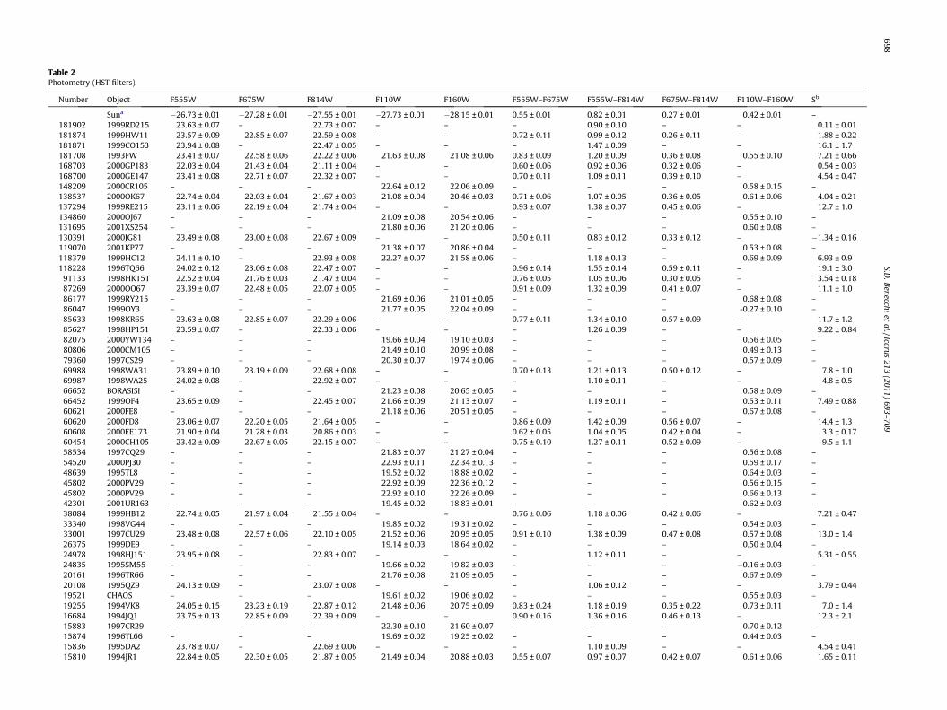
Table 2Photometry (HST filters).
Number Object F555W F675W F814W F110W F160W F555W–F675W F555W–F814W F675W–F814W F110W–F160W Sb
Suna �26.73 ± 0.01 �27.28 ± 0.01 �27.55 ± 0.01 �27.73 ± 0.01 �28.15 ± 0.01 0.55 ± 0.01 0.82 ± 0.01 0.27 ± 0.01 0.42 ± 0.01 –181902 1999RD215 23.63 ± 0.07 – 22.73 ± 0.07 – – – 0.90 ± 0.10 – – 0.11 ± 0.01181874 1999HW11 23.57 ± 0.09 22.85 ± 0.07 22.59 ± 0.08 – – 0.72 ± 0.11 0.99 ± 0.12 0.26 ± 0.11 – 1.88 ± 0.22181871 1999CO153 23.94 ± 0.08 – 22.47 ± 0.05 – – – 1.47 ± 0.09 – – 16.1 ± 1.7181708 1993FW 23.41 ± 0.07 22.58 ± 0.06 22.22 ± 0.06 21.63 ± 0.08 21.08 ± 0.06 0.83 ± 0.09 1.20 ± 0.09 0.36 ± 0.08 0.55 ± 0.10 7.21 ± 0.66168703 2000GP183 22.03 ± 0.04 21.43 ± 0.04 21.11 ± 0.04 – – 0.60 ± 0.06 0.92 ± 0.06 0.32 ± 0.06 – 0.54 ± 0.03168700 2000GE147 23.41 ± 0.08 22.71 ± 0.07 22.32 ± 0.07 – – 0.70 ± 0.11 1.09 ± 0.11 0.39 ± 0.10 – 4.54 ± 0.47148209 2000CR105 – – – 22.64 ± 0.12 22.06 ± 0.09 – – – 0.58 ± 0.15 –138537 2000OK67 22.74 ± 0.04 22.03 ± 0.04 21.67 ± 0.03 21.08 ± 0.04 20.46 ± 0.03 0.71 ± 0.06 1.07 ± 0.05 0.36 ± 0.05 0.61 ± 0.06 4.04 ± 0.21137294 1999RE215 23.11 ± 0.06 22.19 ± 0.04 21.74 ± 0.04 – – 0.93 ± 0.07 1.38 ± 0.07 0.45 ± 0.06 – 12.7 ± 1.0134860 2000OJ67 – – – 21.09 ± 0.08 20.54 ± 0.06 – – – 0.55 ± 0.10 –131695 2001XS254 – – – 21.80 ± 0.06 21.20 ± 0.06 – – – 0.60 ± 0.08 –130391 2000JG81 23.49 ± 0.08 23.00 ± 0.08 22.67 ± 0.09 – – 0.50 ± 0.11 0.83 ± 0.12 0.33 ± 0.12 – �1.34 ± 0.16119070 2001KP77 – – – 21.38 ± 0.07 20.86 ± 0.04 – – – 0.53 ± 0.08 –118379 1999HC12 24.11 ± 0.10 – 22.93 ± 0.08 22.27 ± 0.07 21.58 ± 0.06 – 1.18 ± 0.13 – 0.69 ± 0.09 6.93 ± 0.9118228 1996TQ66 24.02 ± 0.12 23.06 ± 0.08 22.47 ± 0.07 – – 0.96 ± 0.14 1.55 ± 0.14 0.59 ± 0.11 – 19.1 ± 3.0
91133 1998HK151 22.52 ± 0.04 21.76 ± 0.03 21.47 ± 0.04 – – 0.76 ± 0.05 1.05 ± 0.06 0.30 ± 0.05 – 3.54 ± 0.1887269 2000OO67 23.39 ± 0.07 22.48 ± 0.05 22.07 ± 0.05 – – 0.91 ± 0.09 1.32 ± 0.09 0.41 ± 0.07 – 11.1 ± 1.086177 1999RY215 – – – 21.69 ± 0.06 21.01 ± 0.05 – – – 0.68 ± 0.08 –86047 1999OY3 – – – 21.77 ± 0.05 22.04 ± 0.09 – – – -0.27 ± 0.10 –85633 1998KR65 23.63 ± 0.08 22.85 ± 0.07 22.29 ± 0.06 – – 0.77 ± 0.11 1.34 ± 0.10 0.57 ± 0.09 – 11.7 ± 1.285627 1998HP151 23.59 ± 0.07 – 22.33 ± 0.06 – – – 1.26 ± 0.09 – – 9.22 ± 0.8482075 2000YW134 – – – 19.66 ± 0.04 19.10 ± 0.03 – – – 0.56 ± 0.05 –80806 2000CM105 – – – 21.49 ± 0.10 20.99 ± 0.08 – – – 0.49 ± 0.13 –79360 1997CS29 – – – 20.30 ± 0.07 19.74 ± 0.06 – – – 0.57 ± 0.09 –69988 1998WA31 23.89 ± 0.10 23.19 ± 0.09 22.68 ± 0.08 – – 0.70 ± 0.13 1.21 ± 0.13 0.50 ± 0.12 – 7.8 ± 1.069987 1998WA25 24.02 ± 0.08 – 22.92 ± 0.07 – – – 1.10 ± 0.11 – – 4.8 ± 0.566652 BORASISI – – – 21.23 ± 0.08 20.65 ± 0.05 – – – 0.58 ± 0.09 –66452 1999OF4 23.65 ± 0.09 – 22.45 ± 0.07 21.66 ± 0.09 21.13 ± 0.07 – 1.19 ± 0.11 – 0.53 ± 0.11 7.49 ± 0.8860621 2000FE8 – – – 21.18 ± 0.06 20.51 ± 0.05 – – – 0.67 ± 0.08 –60620 2000FD8 23.06 ± 0.07 22.20 ± 0.05 21.64 ± 0.05 – – 0.86 ± 0.09 1.42 ± 0.09 0.56 ± 0.07 – 14.4 ± 1.360608 2000EE173 21.90 ± 0.04 21.28 ± 0.03 20.86 ± 0.03 – – 0.62 ± 0.05 1.04 ± 0.05 0.42 ± 0.04 – 3.3 ± 0.1760454 2000CH105 23.42 ± 0.09 22.67 ± 0.05 22.15 ± 0.07 – – 0.75 ± 0.10 1.27 ± 0.11 0.52 ± 0.09 – 9.5 ± 1.158534 1997CQ29 – – – 21.83 ± 0.07 21.27 ± 0.04 – – – 0.56 ± 0.08 –54520 2000PJ30 – – – 22.93 ± 0.11 22.34 ± 0.13 – – – 0.59 ± 0.17 –48639 1995TL8 – – – 19.52 ± 0.02 18.88 ± 0.02 – – – 0.64 ± 0.03 –45802 2000PV29 – – – 22.92 ± 0.09 22.36 ± 0.12 – – – 0.56 ± 0.15 –45802 2000PV29 – – – 22.92 ± 0.10 22.26 ± 0.09 – – – 0.66 ± 0.13 –42301 2001UR163 – – – 19.45 ± 0.02 18.83 ± 0.01 – – – 0.62 ± 0.03 –38084 1999HB12 22.74 ± 0.05 21.97 ± 0.04 21.55 ± 0.04 – – 0.76 ± 0.06 1.18 ± 0.06 0.42 ± 0.06 – 7.21 ± 0.4733340 1998VG44 – – – 19.85 ± 0.02 19.31 ± 0.02 – – – 0.54 ± 0.03 –33001 1997CU29 23.48 ± 0.08 22.57 ± 0.06 22.10 ± 0.05 21.52 ± 0.06 20.95 ± 0.05 0.91 ± 0.10 1.38 ± 0.09 0.47 ± 0.08 0.57 ± 0.08 13.0 ± 1.426375 1999DE9 – – – 19.14 ± 0.03 18.64 ± 0.02 – – – 0.50 ± 0.04 –24978 1998HJ151 23.95 ± 0.08 – 22.83 ± 0.07 – – – 1.12 ± 0.11 – – 5.31 ± 0.5524835 1995SM55 – – – 19.66 ± 0.02 19.82 ± 0.03 – – – �0.16 ± 0.03 –20161 1996TR66 – – – 21.76 ± 0.08 21.09 ± 0.05 – – – 0.67 ± 0.09 –20108 1995QZ9 24.13 ± 0.09 – 23.07 ± 0.08 – – – 1.06 ± 0.12 – – 3.79 ± 0.4419521 CHAOS – – – 19.61 ± 0.02 19.06 ± 0.02 – – – 0.55 ± 0.03 –19255 1994VK8 24.05 ± 0.15 23.23 ± 0.19 22.87 ± 0.12 21.48 ± 0.06 20.75 ± 0.09 0.83 ± 0.24 1.18 ± 0.19 0.35 ± 0.22 0.73 ± 0.11 7.0 ± 1.416684 1994JQ1 23.75 ± 0.13 22.85 ± 0.09 22.39 ± 0.09 – – 0.90 ± 0.16 1.36 ± 0.16 0.46 ± 0.13 – 12.3 ± 2.115883 1997CR29 – – – 22.30 ± 0.10 21.60 ± 0.07 – – – 0.70 ± 0.12 –15874 1996TL66 – – – 19.69 ± 0.02 19.25 ± 0.02 – – – 0.44 ± 0.03 –15836 1995DA2 23.78 ± 0.07 – 22.69 ± 0.06 – – – 1.10 ± 0.09 – – 4.54 ± 0.4115810 1994JR1 22.84 ± 0.05 22.30 ± 0.05 21.87 ± 0.05 21.49 ± 0.04 20.88 ± 0.03 0.55 ± 0.07 0.97 ± 0.07 0.42 ± 0.07 0.61 ± 0.06 1.65 ± 0.11
698S.D
.Benecchiet
al./Icarus213
(2011)693–
709
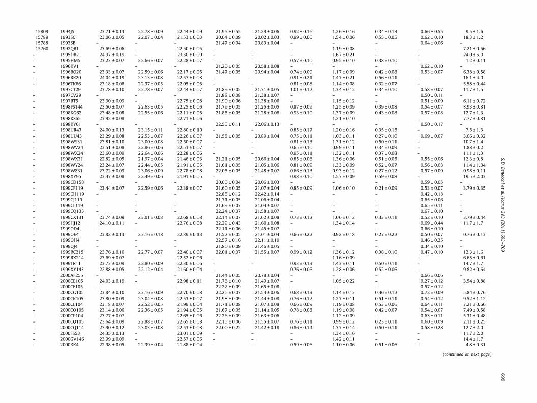
Table 2 (continued)
Number Object F555W F675W F814W F110W F160W F555W–F675W F555W–F814W F675W–F814W F110W–F160W Sb
15809 1994JS 23.71 ± 0.13 22.78 ± 0.09 22.44 ± 0.09 21.95 ± 0.55 21.29 ± 0.06 0.92 ± 0.16 1.26 ± 0.16 0.34 ± 0.13 0.66 ± 0.55 9.5 ± 1.615789 1993SC 23.06 ± 0.05 22.07 ± 0.04 21.53 ± 0.03 20.64 ± 0.09 20.02 ± 0.03 0.99 ± 0.06 1.54 ± 0.06 0.55 ± 0.05 0.62 ± 0.10 18.3 ± 1.215788 1993SB – – – 21.47 ± 0.04 20.83 ± 0.04 – – – 0.64 ± 0.06 –15760 1992QB1 23.69 ± 0.06 – 22.50 ± 0.05 – – – 1.19 ± 0.08 – – 7.21 ± 0.56
– 1995DB2 24.97 ± 0.19 – 23.30 ± 0.09 – – – 1.67 ± 0.21 – – 24.0 ± 6.0– 1995HM5 23.23 ± 0.07 22.66 ± 0.07 22.28 ± 0.07 – – 0.57 ± 0.10 0.95 ± 0.10 0.38 ± 0.10 – 1.2 ± 0.11– 1996KV1 – – – 21.20 ± 0.05 20.58 ± 0.08 – – – 0.62 ± 0.10 –– 1996RQ20 23.33 ± 0.07 22.59 ± 0.06 22.17 ± 0.05 21.47 ± 0.05 20.94 ± 0.04 0.74 ± 0.09 1.17 ± 0.09 0.42 ± 0.08 0.53 ± 0.07 6.38 ± 0.58– 1996RR20 24.04 ± 0.19 23.13 ± 0.08 22.57 ± 0.08 – – 0.91 ± 0.21 1.47 ± 0.21 0.56 ± 0.11 – 16.1 ± 4.0– 1996TK66 23.18 ± 0.06 22.37 ± 0.05 22.05 ± 0.05 – – 0.81 ± 0.08 1.14 ± 0.08 0.32 ± 0.07 – 5.58 ± 0.44– 1997CT29 23.78 ± 0.10 22.78 ± 0.07 22.44 ± 0.07 21.89 ± 0.05 21.31 ± 0.05 1.01 ± 0.12 1.34 ± 0.12 0.34 ± 0.10 0.58 ± 0.07 11.7 ± 1.5– 1997CV29 – – – 21.88 ± 0.08 21.38 ± 0.07 – – – 0.50 ± 0.11 –– 1997RT5 23.90 ± 0.09 – 22.75 ± 0.08 21.90 ± 0.06 21.38 ± 0.06 – 1.15 ± 0.12 – 0.51 ± 0.09 6.11 ± 0.72– 1998FS144 23.50 ± 0.07 22.63 ± 0.05 22.25 ± 0.06 21.79 ± 0.05 21.25 ± 0.05 0.87 ± 0.09 1.25 ± 0.09 0.39 ± 0.08 0.54 ± 0.07 8.93 ± 0.81– 1998KG62 23.48 ± 0.08 22.55 ± 0.06 22.11 ± 0.05 21.85 ± 0.05 21.28 ± 0.06 0.93 ± 0.10 1.37 ± 0.09 0.43 ± 0.08 0.57 ± 0.08 12.7 ± 1.3– 1998KS65 23.92 ± 0.08 – 22.71 ± 0.06 – – – 1.21 ± 0.10 – – 7.77 ± 0.81– 1998KY61 – – – 22.55 ± 0.11 22.06 ± 0.13 – – – 0.50 ± 0.17 –– 1998UR43 24.00 ± 0.13 23.15 ± 0.11 22.80 ± 0.10 – – 0.85 ± 0.17 1.20 ± 0.16 0.35 ± 0.15 – 7.5 ± 1.3– 1998UU43 23.29 ± 0.08 22.53 ± 0.07 22.26 ± 0.07 21.58 ± 0.05 20.89 ± 0.04 0.75 ± 0.11 1.03 ± 0.11 0.27 ± 0.10 0.69 ± 0.07 3.06 ± 0.32– 1998WS31 23.81 ± 0.10 23.00 ± 0.08 22.50 ± 0.07 – – 0.81 ± 0.13 1.31 ± 0.12 0.50 ± 0.11 – 10.7 ± 1.4– 1998WV24 23.51 ± 0.08 22.86 ± 0.06 22.53 ± 0.07 – – 0.65 ± 0.10 0.99 ± 0.11 0.34 ± 0.09 – 1.88 ± 0.2– 1998WX24 23.60 ± 0.09 22.64 ± 0.06 22.28 ± 0.06 – – 0.95 ± 0.11 1.32 ± 0.11 0.37 ± 0.08 – 11.1 ± 1.3– 1998WX31 22.82 ± 0.05 21.97 ± 0.04 21.46 ± 0.03 21.21 ± 0.05 20.66 ± 0.04 0.85 ± 0.06 1.36 ± 0.06 0.51 ± 0.05 0.55 ± 0.06 12.3 ± 0.8– 1998WY24 23.24 ± 0.07 22.44 ± 0.05 21.91 ± 0.05 21.61 ± 0.05 21.05 ± 0.06 0.81 ± 0.09 1.33 ± 0.09 0.52 ± 0.07 0.56 ± 0.08 11.4 ± 1.04– 1998WZ31 23.72 ± 0.09 23.06 ± 0.09 22.78 ± 0.08 22.05 ± 0.05 21.48 ± 0.07 0.66 ± 0.13 0.93 ± 0.12 0.27 ± 0.12 0.57 ± 0.09 0.98 ± 0.11– 1998XY95 23.47 ± 0.08 22.49 ± 0.06 21.91 ± 0.05 – – 0.98 ± 0.10 1.57 ± 0.09 0.59 ± 0.08 – 19.5 ± 2.03– 1999CD158 – – – 20.66 ± 0.04 20.06 ± 0.03 – – – 0.59 ± 0.05 –– 1999CF119 23.44 ± 0.07 22.59 ± 0.06 22.38 ± 0.07 21.60 ± 0.05 21.07 ± 0.04 0.85 ± 0.09 1.06 ± 0.10 0.21 ± 0.09 0.53 ± 0.07 3.79 ± 0.35– 1999CH119 – – – 22.85 ± 0.12 22.42 ± 0.14 – – – 0.42 ± 0.18 –– 1999CJ119 – – – 21.71 ± 0.05 21.06 ± 0.04 – – – 0.65 ± 0.06 –– 1999CL119 – – – 21.69 ± 0.07 21.04 ± 0.07 – – – 0.65 ± 0.11 –– 1999CQ133 – – – 22.24 ± 0.07 21.58 ± 0.07 – – – 0.67 ± 0.10 –– 1999CX131 23.74 ± 0.09 23.01 ± 0.08 22.68 ± 0.08 22.14 ± 0.07 21.62 ± 0.08 0.73 ± 0.12 1.06 ± 0.12 0.33 ± 0.11 0.52 ± 0.10 3.79 ± 0.44– 1999HJ12 24.10 ± 0.11 – 22.76 ± 0.08 22.29 ± 0.43 21.60 ± 0.08 – 1.34 ± 0.14 – 0.69 ± 0.44 11.7 ± 1.7– 1999OD4 – – – 22.11 ± 0.06 21.45 ± 0.07 – – – 0.66 ± 0.10 –– 1999OE4 23.82 ± 0.13 23.16 ± 0.18 22.89 ± 0.13 21.52 ± 0.05 21.01 ± 0.04 0.66 ± 0.22 0.92 ± 0.18 0.27 ± 0.22 0.50 ± 0.07 0.76 ± 0.13– 1999OH4 – – – 22.57 ± 0.16 22.11 ± 0.19 – – – 0.46 ± 0.25 –– 1999OJ4 – – – 21.80 ± 0.09 21.46 ± 0.05 – – – 0.34 ± 0.10 –– 1999RC215 23.76 ± 0.10 22.77 ± 0.07 22.40 ± 0.07 22.01 ± 0.07 21.55 ± 0.07 0.99 ± 0.12 1.36 ± 0.12 0.38 ± 0.10 0.47 ± 0.10 12.3 ± 1.6– 1999RX214 23.69 ± 0.07 – 22.52 ± 0.06 – – – 1.16 ± 0.09 – – 6.65 ± 0.61– 1999TR11 23.73 ± 0.09 22.80 ± 0.09 22.30 ± 0.06 – – 0.93 ± 0.13 1.43 ± 0.11 0.50 ± 0.11 – 14.7 ± 1.7– 1999XY143 22.88 ± 0.05 22.12 ± 0.04 21.60 ± 0.04 – – 0.76 ± 0.06 1.28 ± 0.06 0.52 ± 0.06 – 9.82 ± 0.64– 2000AF255 – – – 21.44 ± 0.05 20.78 ± 0.04 – – – 0.66 ± 0.06 –– 2000CE105 24.03 ± 0.19 – 22.98 ± 0.11 21.76 ± 0.10 21.49 ± 0.07 – 1.05 ± 0.22 – 0.27 ± 0.12 3.54 ± 0.88– 2000CF105 – – – 22.22 ± 0.09 21.65 ± 0.08 – – – 0.57 ± 0.12 –– 2000CG105 23.84 ± 0.10 23.16 ± 0.09 22.70 ± 0.08 22.26 ± 0.07 21.54 ± 0.06 0.68 ± 0.13 1.14 ± 0.13 0.46 ± 0.12 0.72 ± 0.09 5.84 ± 0.76– 2000CK105 23.80 ± 0.09 23.04 ± 0.08 22.53 ± 0.07 21.98 ± 0.09 21.44 ± 0.08 0.76 ± 0.12 1.27 ± 0.11 0.51 ± 0.11 0.54 ± 0.12 9.52 ± 1.12– 2000CL104 23.18 ± 0.07 22.52 ± 0.05 21.99 ± 0.04 21.71 ± 0.08 21.07 ± 0.08 0.66 ± 0.09 1.19 ± 0.08 0.53 ± 0.06 0.64 ± 0.11 7.21 ± 0.66– 2000CO105 23.14 ± 0.06 22.36 ± 0.05 21.94 ± 0.05 21.67 ± 0.05 21.14 ± 0.05 0.78 ± 0.08 1.19 ± 0.08 0.42 ± 0.07 0.54 ± 0.07 7.49 ± 0.58– 2000CP104 23.77 ± 0.07 – 22.65 ± 0.06 22.26 ± 0.09 21.63 ± 0.06 – 1.12 ± 0.09 – 0.63 ± 0.11 5.31 ± 0.48– 2000CQ105 23.64 ± 0.09 22.88 ± 0.07 22.65 ± 0.08 22.15 ± 0.06 21.55 ± 0.07 0.76 ± 0.11 0.99 ± 0.12 0.23 ± 0.11 0.60 ± 0.09 2.11 ± 0.25– 2000CQ114 23.90 ± 0.12 23.03 ± 0.08 22.53 ± 0.08 22.00 ± 0.22 21.42 ± 0.18 0.86 ± 0.14 1.37 ± 0.14 0.50 ± 0.11 0.58 ± 0.28 12.7 ± 2.0– 2000FS53 24.35 ± 0.13 – 23.01 ± 0.09 – – – 1.34 ± 0.16 – – 11.7 ± 2.0– 2000GV146 23.99 ± 0.09 – 22.57 ± 0.06 – – – 1.42 ± 0.11 – – 14.4 ± 1.7– 2000KK4 22.98 ± 0.05 22.39 ± 0.04 21.88 ± 0.04 – – 0.59 ± 0.06 1.10 ± 0.06 0.51 ± 0.06 – 4.8 ± 0.31
(continued on next page)
S.D.Benecchi
etal./Icarus
213(2011)
693–709
699
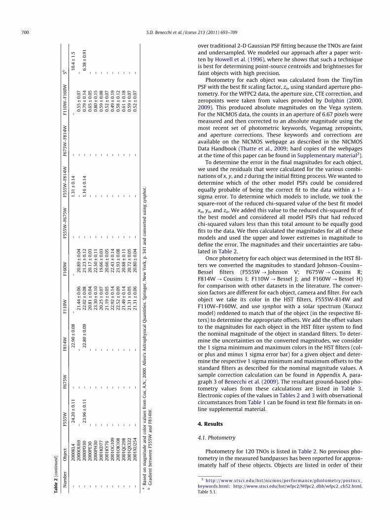
Tabl
e2
(con
tinu
ed)
Nu
mbe
rO
bjec
tF5
55W
F675
WF8
14W
F110
WF1
60W
F555
W–F
675W
F555
W–F
814W
F675
W–F
814W
F110
W–F
160W
Sb
–20
00K
L424
.20
±0.
11–
22.9
0±
0.08
––
–1.
31±
0.14
––
10.4
±1.
5–
2000
OU
69–
––
21.4
4±
0.06
20.8
9±
0.04
––
–0.
55±
0.07
––
2000
PD30
23.9
6±
0.11
–22
.80
±0.
0922
.02
±0.
0821
.23
±0.
12–
1.16
±0.
14–
0.79
±0.
146.
38±
0.91
–20
00PE
30–
––
20.8
1±
0.04
20.1
7±
0.03
––
–0.
65±
0.05
––
2000
PH30
––
–23
.30
±0.
1022
.50
±0.
11–
––
0.80
±0.
15–
–20
01K
D77
––
–20
.25
±0.
0719
.66
±0.
03–
––
0.59
±0.
08–
–20
01K
Y76
––
–21
.19
±0.
0520
.66
±0.
05–
––
0.52
±0.
07–
–20
01O
G10
9–
––
22.9
2±
0.14
22.4
3±
0.14
––
–0.
49±
0.19
––
2001
OK
108
––
–22
.52
±0.
0921
.93
±0.
08–
––
0.58
±0.
12–
–20
01Q
C29
8–
––
21.4
9±
0.14
20.8
8±
0.11
––
–0.
61±
0.18
––
2001
QX
322
––
–21
.31
±0.
0520
.72
±0.
05–
––
0.59
±0.
07–
–20
01X
U25
4–
––
21.3
1±
0.06
20.8
0±
0.04
––
–0.
52±
0.07
–
aB
ased
onm
agn
itu
dean
dco
lor
valu
esfr
omC
ox,A
.N.,
2000
.All
en’s
Ast
roph
ysic
alQ
uan
titi
es.S
prin
ger,
New
Yor
k,p.
341
and
con
vert
edu
sin
gsy
npho
t.b
Gra
dien
tbe
twee
nF5
55W
and
F814
W.
2 http://www.stsci.edu/hst/nicmos/performance/photometry/postncs_keywords.html; http://www.stsci.edu/hst/wfpc2/Wfpc2_dhb/wfpc2_ch52.html,Table 5.1.
700 S.D. Benecchi et al. / Icarus 213 (2011) 693–709
over traditional 2-D Gaussian PSF fitting because the TNOs are faintand undersampled. We modeled our approach after a paper writ-ten by Howell et al. (1996), where he shows that such a techniqueis best for determining point-source centroids and brightnesses forfaint objects with high precision.
Photometry for each object was calculated from the TinyTimPSF with the best fit scaling factor, zo, using standard aperture pho-tometry. For the WFPC2 data, the aperture size, CTE correction, andzeropoints were taken from values provided by Dolphin (2000,2009). This produced absolute magnitudes on the Vega system.For the NICMOS data, the counts in an aperture of 6.67 pixels weremeasured and then corrected to an absolute magnitude using themost recent set of photometric keywords, Vegamag zeropoints,and aperture corrections. These keywords and corrections areavailable on the NICMOS webpage as described in the NICMOSData Handbook (Thatte et al., 2009; hard copies of the webpagesat the time of this paper can be found in Supplementary material2).
To determine the error in the final magnitudes for each object,we used the residuals that were calculated for the various combi-nations of x, y, and z during the initial fitting process. We wanted todetermine which of the other model PSFs could be consideredequally probable of being the correct fit to the data within a 1-sigma error. To determine which models to include, we took thesquare-root of the reduced chi-squared value of the best fit modelxo, yo, and zo. We added this value to the reduced chi-squared fit ofthe best model and considered all model PSFs that had reducedchi-squared values less than this total amount to be equally goodfits to the data. We then calculated the magnitudes for all of thesemodels and used the upper and lower extremes in magnitude todefine the error. The magnitudes and their uncertainties are tabu-lated in Table 2.
Once photometry for each object was determined in the HST fil-ters we converted the magnitudes to standard Johnson–Cousins–Bessel filters (F555W ? Johnson V; F675W ? Cousins R;F814W ? Cousins I; F110W ? Bessel J; and F160W ? Bessel H)for comparison with other datasets in the literature. The conver-sion factors are different for each object, camera and filter. For eachobject we take its color in the HST filters, F555W-814W andF110W–F160W, and use synphot with a solar spectrum (Kuruczmodel) reddened to match that of the object (in the respective fil-ters) to determine the appropriate offsets. We add the offset valuesto the magnitudes for each object in the HST filter system to findthe nominal magnitude of the object in standard filters. To deter-mine the uncertainties on the converted magnitudes, we considerthe 1 sigma minimum and maximum colors in the HST filters (col-or plus and minus 1 sigma error bar) for a given object and deter-mine the respective 1 sigma minimum and maximum offsets to thestandard filters as described for the nominal magnitude values. Asample correction calculation can be found in Appendix A, para-graph 3 of Benecchi et al. (2009). The resultant ground-based pho-tometry values from these calculations are listed in Table 3.Electronic copies of the values in Tables 2 and 3 with observationalcircumstances from Table 1 can be found in text file formats in on-line supplemental material.
4. Results
4.1. Photometry
Photometry for 120 TNOs is listed in Table 2. No previous pho-tometry in the measured bandpasses has been reported for approx-imately half of these objects. Objects are listed in order of their
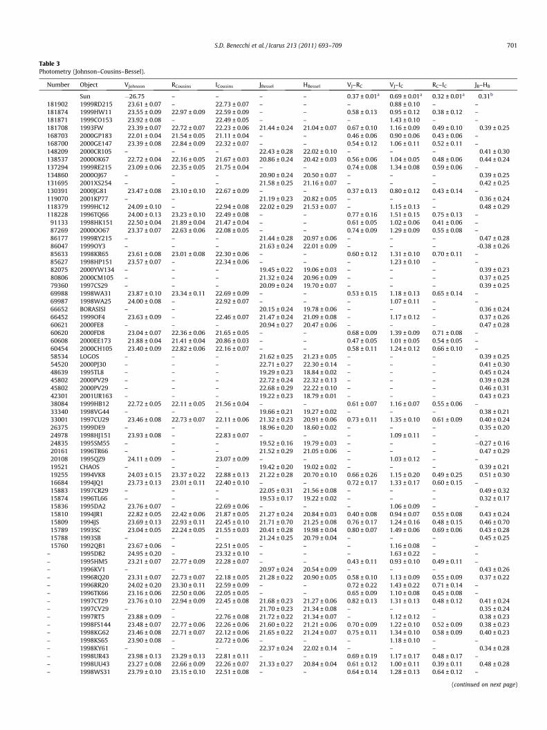
Table 3Photometry (Johnson–Cousins–Bessel).
Number Object VJohnson RCousins ICousins JBessel HBessel VJ–RC VJ–IC RC–IC JB–HB
Sun �26.75 – – – – 0.37 ± 0.01a 0.69 ± 0.01a 0.32 ± 0.01a 0.31b
181902 1999RD215 23.61 ± 0.07 – 22.73 ± 0.07 – – – 0.88 ± 0.10 – –181874 1999HW11 23.55 ± 0.09 22.97 ± 0.09 22.59 ± 0.09 – – 0.58 ± 0.13 0.95 ± 0.12 0.38 ± 0.12 –181871 1999CO153 23.92 ± 0.08 – 22.49 ± 0.05 – – – 1.43 ± 0.10 – –181708 1993FW 23.39 ± 0.07 22.72 ± 0.07 22.23 ± 0.06 21.44 ± 0.24 21.04 ± 0.07 0.67 ± 0.10 1.16 ± 0.09 0.49 ± 0.10 0.39 ± 0.25168703 2000GP183 22.01 ± 0.04 21.54 ± 0.05 21.11 ± 0.04 – – 0.46 ± 0.06 0.90 ± 0.06 0.43 ± 0.06 –168700 2000GE147 23.39 ± 0.08 22.84 ± 0.09 22.32 ± 0.07 – – 0.54 ± 0.12 1.06 ± 0.11 0.52 ± 0.11 –148209 2000CR105 – – – 22.43 ± 0.28 22.02 ± 0.10 – – – 0.41 ± 0.30138537 2000OK67 22.72 ± 0.04 22.16 ± 0.05 21.67 ± 0.03 20.86 ± 0.24 20.42 ± 0.03 0.56 ± 0.06 1.04 ± 0.05 0.48 ± 0.06 0.44 ± 0.24137294 1999RE215 23.09 ± 0.06 22.35 ± 0.05 21.75 ± 0.04 – – 0.74 ± 0.08 1.34 ± 0.08 0.59 ± 0.06 –134860 2000OJ67 – – – 20.90 ± 0.24 20.50 ± 0.07 – – – 0.39 ± 0.25131695 2001XS254 – – – 21.58 ± 0.25 21.16 ± 0.07 – – – 0.42 ± 0.25130391 2000JG81 23.47 ± 0.08 23.10 ± 0.10 22.67 ± 0.09 – – 0.37 ± 0.13 0.80 ± 0.12 0.43 ± 0.14 –119070 2001KP77 – – – 21.19 ± 0.23 20.82 ± 0.05 – – – 0.36 ± 0.24118379 1999HC12 24.09 ± 0.10 – 22.94 ± 0.08 22.02 ± 0.29 21.53 ± 0.07 – 1.15 ± 0.13 – 0.48 ± 0.29118228 1996TQ66 24.00 ± 0.13 23.23 ± 0.10 22.49 ± 0.08 – – 0.77 ± 0.16 1.51 ± 0.15 0.75 ± 0.13 –
91133 1998HK151 22.50 ± 0.04 21.89 ± 0.04 21.47 ± 0.04 – – 0.61 ± 0.05 1.02 ± 0.06 0.41 ± 0.06 –87269 2000OO67 23.37 ± 0.07 22.63 ± 0.06 22.08 ± 0.05 – – 0.74 ± 0.09 1.29 ± 0.09 0.55 ± 0.08 –86177 1999RY215 – – – 21.44 ± 0.28 20.97 ± 0.06 – – – 0.47 ± 0.2886047 1999OY3 – – – 21.63 ± 0.24 22.01 ± 0.09 – – – -0.38 ± 0.2685633 1998KR65 23.61 ± 0.08 23.01 ± 0.08 22.30 ± 0.06 – – 0.60 ± 0.12 1.31 ± 0.10 0.70 ± 0.11 –85627 1998HP151 23.57 ± 0.07 – 22.34 ± 0.06 – – – 1.23 ± 0.10 – –82075 2000YW134 – – – 19.45 ± 0.22 19.06 ± 0.03 – – – 0.39 ± 0.2380806 2000CM105 – – – 21.32 ± 0.24 20.96 ± 0.09 – – – 0.37 ± 0.2579360 1997CS29 – – – 20.09 ± 0.24 19.70 ± 0.07 – – – 0.39 ± 0.2569988 1998WA31 23.87 ± 0.10 23.34 ± 0.11 22.69 ± 0.09 – – 0.53 ± 0.15 1.18 ± 0.13 0.65 ± 0.14 –69987 1998WA25 24.00 ± 0.08 – 22.92 ± 0.07 – – – 1.07 ± 0.11 – –66652 BORASISI – – – 20.15 ± 0.24 19.78 ± 0.06 – – – 0.36 ± 0.2466452 1999OF4 23.63 ± 0.09 – 22.46 ± 0.07 21.47 ± 0.24 21.09 ± 0.08 – 1.17 ± 0.12 – 0.37 ± 0.2660621 2000FE8 – – – 20.94 ± 0.27 20.47 ± 0.06 – – – 0.47 ± 0.2860620 2000FD8 23.04 ± 0.07 22.36 ± 0.06 21.65 ± 0.05 – – 0.68 ± 0.09 1.39 ± 0.09 0.71 ± 0.08 –60608 2000EE173 21.88 ± 0.04 21.41 ± 0.04 20.86 ± 0.03 – – 0.47 ± 0.05 1.01 ± 0.05 0.54 ± 0.05 –60454 2000CH105 23.40 ± 0.09 22.82 ± 0.06 22.16 ± 0.07 – – 0.58 ± 0.11 1.24 ± 0.12 0.66 ± 0.10 –58534 LOGOS – – – 21.62 ± 0.25 21.23 ± 0.05 – – – 0.39 ± 0.2554520 2000PJ30 – – – 22.71 ± 0.27 22.30 ± 0.14 – – – 0.41 ± 0.3048639 1995TL8 – – – 19.29 ± 0.23 18.84 ± 0.02 – – – 0.45 ± 0.2445802 2000PV29 – – – 22.72 ± 0.24 22.32 ± 0.13 – – – 0.39 ± 0.2845802 2000PV29 – – – 22.68 ± 0.29 22.22 ± 0.10 – – – 0.46 ± 0.3142301 2001UR163 – – – 19.22 ± 0.23 18.79 ± 0.01 – – – 0.43 ± 0.2338084 1999HB12 22.72 ± 0.05 22.11 ± 0.05 21.56 ± 0.04 – – 0.61 ± 0.07 1.16 ± 0.07 0.55 ± 0.06 –33340 1998VG44 – – – 19.66 ± 0.21 19.27 ± 0.02 – – – 0.38 ± 0.2133001 1997CU29 23.46 ± 0.08 22.73 ± 0.07 22.11 ± 0.06 21.32 ± 0.23 20.91 ± 0.06 0.73 ± 0.11 1.35 ± 0.10 0.61 ± 0.09 0.40 ± 0.2426375 1999DE9 – – – 18.96 ± 0.20 18.60 ± 0.02 – – – 0.35 ± 0.2024978 1998HJ151 23.93 ± 0.08 – 22.83 ± 0.07 – – – 1.09 ± 0.11 – –24835 1995SM55 – – – 19.52 ± 0.16 19.79 ± 0.03 – – – �0.27 ± 0.1620161 1996TR66 – – – 21.52 ± 0.29 21.05 ± 0.06 – – – 0.47 ± 0.2920108 1995QZ9 24.11 ± 0.09 – 23.07 ± 0.09 – – – 1.03 ± 0.12 – –19521 CHAOS – – – 19.42 ± 0.20 19.02 ± 0.02 – – – 0.39 ± 0.2119255 1994VK8 24.03 ± 0.15 23.37 ± 0.22 22.88 ± 0.13 21.22 ± 0.28 20.70 ± 0.10 0.66 ± 0.26 1.15 ± 0.20 0.49 ± 0.25 0.51 ± 0.3016684 1994JQ1 23.73 ± 0.13 23.01 ± 0.11 22.40 ± 0.10 – – 0.72 ± 0.17 1.33 ± 0.17 0.60 ± 0.15 –15883 1997CR29 – – – 22.05 ± 0.31 21.56 ± 0.08 – – – 0.49 ± 0.3215874 1996TL66 – – – 19.53 ± 0.17 19.22 ± 0.02 – – – 0.32 ± 0.1715836 1995DA2 23.76 ± 0.07 – 22.69 ± 0.06 – – – 1.06 ± 0.09 – –15810 1994JR1 22.82 ± 0.05 22.42 ± 0.06 21.87 ± 0.05 21.27 ± 0.24 20.84 ± 0.03 0.40 ± 0.08 0.94 ± 0.07 0.55 ± 0.08 0.43 ± 0.2415809 1994JS 23.69 ± 0.13 22.93 ± 0.11 22.45 ± 0.10 21.71 ± 0.70 21.25 ± 0.08 0.76 ± 0.17 1.24 ± 0.16 0.48 ± 0.15 0.46 ± 0.7015789 1993SC 23.04 ± 0.05 22.24 ± 0.05 21.55 ± 0.03 20.41 ± 0.28 19.98 ± 0.04 0.80 ± 0.07 1.49 ± 0.06 0.69 ± 0.06 0.43 ± 0.2815788 1993SB – – – 21.24 ± 0.25 20.79 ± 0.04 – – – 0.45 ± 0.2515760 1992QB1 23.67 ± 0.06 – 22.51 ± 0.05 – – – 1.16 ± 0.08 – –
– 1995DB2 24.95 ± 0.20 – 23.32 ± 0.10 – – – 1.63 ± 0.22 – –– 1995HM5 23.21 ± 0.07 22.77 ± 0.09 22.28 ± 0.07 – – 0.43 ± 0.11 0.93 ± 0.10 0.49 ± 0.11 –– 1996KV1 – – – 20.97 ± 0.24 20.54 ± 0.09 – – – 0.43 ± 0.26– 1996RQ20 23.31 ± 0.07 22.73 ± 0.07 22.18 ± 0.05 21.28 ± 0.22 20.90 ± 0.05 0.58 ± 0.10 1.13 ± 0.09 0.55 ± 0.09 0.37 ± 0.22– 1996RR20 24.02 ± 0.20 23.30 ± 0.11 22.59 ± 0.09 – – 0.72 ± 0.22 1.43 ± 0.22 0.71 ± 0.14 –– 1996TK66 23.16 ± 0.06 22.50 ± 0.06 22.05 ± 0.05 – – 0.65 ± 0.09 1.10 ± 0.08 0.45 ± 0.08 –– 1997CT29 23.76 ± 0.10 22.94 ± 0.09 22.45 ± 0.08 21.68 ± 0.23 21.27 ± 0.06 0.82 ± 0.13 1.31 ± 0.13 0.48 ± 0.12 0.41 ± 0.24– 1997CV29 – – – 21.70 ± 0.23 21.34 ± 0.08 – – – 0.35 ± 0.24– 1997RT5 23.88 ± 0.09 – 22.76 ± 0.08 21.72 ± 0.22 21.34 ± 0.07 – 1.12 ± 0.12 – 0.38 ± 0.23– 1998FS144 23.48 ± 0.07 22.77 ± 0.06 22.26 ± 0.06 21.60 ± 0.22 21.21 ± 0.06 0.70 ± 0.09 1.22 ± 0.10 0.52 ± 0.09 0.38 ± 0.23– 1998KG62 23.46 ± 0.08 22.71 ± 0.07 22.12 ± 0.06 21.65 ± 0.22 21.24 ± 0.07 0.75 ± 0.11 1.34 ± 0.10 0.58 ± 0.09 0.40 ± 0.23– 1998KS65 23.90 ± 0.08 – 22.72 ± 0.06 – – – 1.18 ± 0.10 – –– 1998KY61 – – – 22.37 ± 0.24 22.02 ± 0.14 – – – 0.34 ± 0.28– 1998UR43 23.98 ± 0.13 23.29 ± 0.13 22.81 ± 0.11 – – 0.69 ± 0.19 1.17 ± 0.17 0.48 ± 0.17 –– 1998UU43 23.27 ± 0.08 22.66 ± 0.09 22.26 ± 0.07 21.33 ± 0.27 20.84 ± 0.04 0.61 ± 0.12 1.00 ± 0.11 0.39 ± 0.11 0.48 ± 0.28– 1998WS31 23.79 ± 0.10 23.15 ± 0.10 22.51 ± 0.08 – – 0.64 ± 0.14 1.28 ± 0.13 0.64 ± 0.12 –
(continued on next page)
S.D. Benecchi et al. / Icarus 213 (2011) 693–709 701
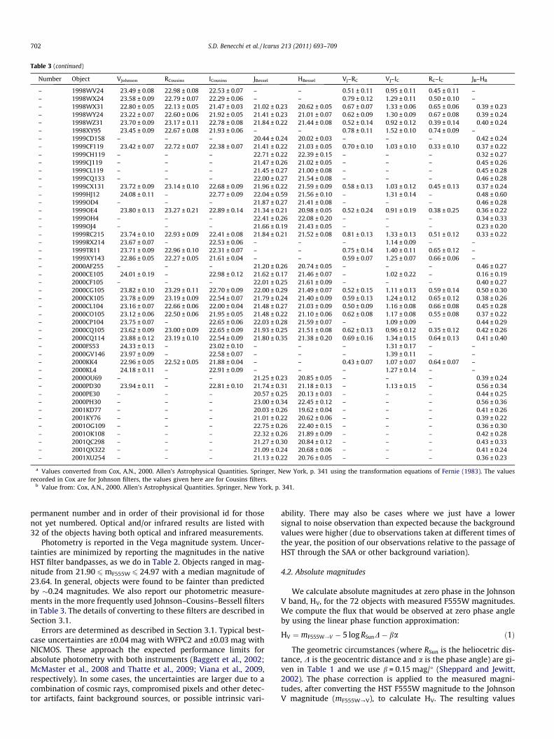
Table 3 (continued)
Number Object VJohnson RCousins ICousins JBessel HBessel VJ–RC VJ–IC RC–IC JB–HB
– 1998WV24 23.49 ± 0.08 22.98 ± 0.08 22.53 ± 0.07 – – 0.51 ± 0.11 0.95 ± 0.11 0.45 ± 0.11 –– 1998WX24 23.58 ± 0.09 22.79 ± 0.07 22.29 ± 0.06 – – 0.79 ± 0.12 1.29 ± 0.11 0.50 ± 0.10 –– 1998WX31 22.80 ± 0.05 22.13 ± 0.05 21.47 ± 0.03 21.02 ± 0.23 20.62 ± 0.05 0.67 ± 0.07 1.33 ± 0.06 0.65 ± 0.06 0.39 ± 0.23– 1998WY24 23.22 ± 0.07 22.60 ± 0.06 21.92 ± 0.05 21.41 ± 0.23 21.01 ± 0.07 0.62 ± 0.09 1.30 ± 0.09 0.67 ± 0.08 0.39 ± 0.24– 1998WZ31 23.70 ± 0.09 23.17 ± 0.11 22.78 ± 0.08 21.84 ± 0.22 21.44 ± 0.08 0.52 ± 0.14 0.92 ± 0.12 0.39 ± 0.14 0.40 ± 0.24– 1998XY95 23.45 ± 0.09 22.67 ± 0.08 21.93 ± 0.06 – – 0.78 ± 0.11 1.52 ± 0.10 0.74 ± 0.09 –– 1999CD158 – – – 20.44 ± 0.24 20.02 ± 0.03 – – – 0.42 ± 0.24– 1999CF119 23.42 ± 0.07 22.72 ± 0.07 22.38 ± 0.07 21.41 ± 0.22 21.03 ± 0.05 0.70 ± 0.10 1.03 ± 0.10 0.33 ± 0.10 0.37 ± 0.22– 1999CH119 – – – 22.71 ± 0.22 22.39 ± 0.15 – – – 0.32 ± 0.27– 1999CJ119 – – – 21.47 ± 0.26 21.02 ± 0.05 – – – 0.45 ± 0.26– 1999CL119 – – – 21.45 ± 0.27 21.00 ± 0.08 – – – 0.45 ± 0.28– 1999CQ133 – – – 22.00 ± 0.27 21.54 ± 0.08 – – – 0.46 ± 0.28– 1999CX131 23.72 ± 0.09 23.14 ± 0.10 22.68 ± 0.09 21.96 ± 0.22 21.59 ± 0.09 0.58 ± 0.13 1.03 ± 0.12 0.45 ± 0.13 0.37 ± 0.24– 1999HJ12 24.08 ± 0.11 – 22.77 ± 0.09 22.04 ± 0.59 21.56 ± 0.10 – 1.31 ± 0.14 – 0.48 ± 0.60– 1999OD4 – – – 21.87 ± 0.27 21.41 ± 0.08 – – – 0.46 ± 0.28– 1999OE4 23.80 ± 0.13 23.27 ± 0.21 22.89 ± 0.14 21.34 ± 0.21 20.98 ± 0.05 0.52 ± 0.24 0.91 ± 0.19 0.38 ± 0.25 0.36 ± 0.22– 1999OH4 – – – 22.41 ± 0.26 22.08 ± 0.20 – – – 0.34 ± 0.33– 1999OJ4 – – – 21.66 ± 0.19 21.43 ± 0.05 – – – 0.23 ± 0.20– 1999RC215 23.74 ± 0.10 22.93 ± 0.09 22.41 ± 0.08 21.84 ± 0.21 21.52 ± 0.08 0.81 ± 0.13 1.33 ± 0.13 0.51 ± 0.12 0.33 ± 0.22– 1999RX214 23.67 ± 0.07 – 22.53 ± 0.06 – – – 1.14 ± 0.09 – –– 1999TR11 23.71 ± 0.09 22.96 ± 0.10 22.31 ± 0.07 – – 0.75 ± 0.14 1.40 ± 0.11 0.65 ± 0.12 –– 1999XY143 22.86 ± 0.05 22.27 ± 0.05 21.61 ± 0.04 – – 0.59 ± 0.07 1.25 ± 0.07 0.66 ± 0.06 –– 2000AF255 – – – 21.20 ± 0.26 20.74 ± 0.05 – – – 0.46 ± 0.27– 2000CE105 24.01 ± 0.19 – 22.98 ± 0.12 21.62 ± 0.17 21.46 ± 0.07 – 1.02 ± 0.22 – 0.16 ± 0.19– 2000CF105 – – – 22.01 ± 0.25 21.61 ± 0.09 – – – 0.40 ± 0.27– 2000CG105 23.82 ± 0.10 23.29 ± 0.11 22.70 ± 0.09 22.00 ± 0.29 21.49 ± 0.07 0.52 ± 0.15 1.11 ± 0.13 0.59 ± 0.14 0.50 ± 0.30– 2000CK105 23.78 ± 0.09 23.19 ± 0.09 22.54 ± 0.07 21.79 ± 0.24 21.40 ± 0.09 0.59 ± 0.13 1.24 ± 0.12 0.65 ± 0.12 0.38 ± 0.26– 2000CL104 23.16 ± 0.07 22.66 ± 0.06 22.00 ± 0.04 21.48 ± 0.27 21.03 ± 0.09 0.50 ± 0.09 1.16 ± 0.08 0.66 ± 0.08 0.45 ± 0.28– 2000CO105 23.12 ± 0.06 22.50 ± 0.06 21.95 ± 0.05 21.48 ± 0.22 21.10 ± 0.06 0.62 ± 0.08 1.17 ± 0.08 0.55 ± 0.08 0.37 ± 0.22– 2000CP104 23.75 ± 0.07 – 22.65 ± 0.06 22.03 ± 0.28 21.59 ± 0.07 – 1.09 ± 0.09 – 0.44 ± 0.29– 2000CQ105 23.62 ± 0.09 23.00 ± 0.09 22.65 ± 0.09 21.93 ± 0.25 21.51 ± 0.08 0.62 ± 0.13 0.96 ± 0.12 0.35 ± 0.12 0.42 ± 0.26– 2000CQ114 23.88 ± 0.12 23.19 ± 0.10 22.54 ± 0.09 21.80 ± 0.35 21.38 ± 0.20 0.69 ± 0.16 1.34 ± 0.15 0.64 ± 0.13 0.41 ± 0.40– 2000FS53 24.33 ± 0.13 – 23.02 ± 0.10 – – – 1.31 ± 0.17 – –– 2000GV146 23.97 ± 0.09 – 22.58 ± 0.07 – – – 1.39 ± 0.11 – –– 2000KK4 22.96 ± 0.05 22.52 ± 0.05 21.88 ± 0.04 – – 0.43 ± 0.07 1.07 ± 0.07 0.64 ± 0.07 –– 2000KL4 24.18 ± 0.11 – 22.91 ± 0.09 – – – 1.27 ± 0.14 – –– 2000OU69 – – – 21.25 ± 0.23 20.85 ± 0.05 – – – 0.39 ± 0.24– 2000PD30 23.94 ± 0.11 – 22.81 ± 0.10 21.74 ± 0.31 21.18 ± 0.13 – 1.13 ± 0.15 – 0.56 ± 0.34– 2000PE30 – – – 20.57 ± 0.25 20.13 ± 0.03 – – – 0.44 ± 0.25– 2000PH30 – – – 23.00 ± 0.34 22.45 ± 0.12 – – – 0.56 ± 0.36– 2001KD77 – – – 20.03 ± 0.26 19.62 ± 0.04 – – – 0.41 ± 0.26– 2001KY76 – – – 21.01 ± 0.22 20.62 ± 0.06 – – – 0.39 ± 0.22– 2001OG109 – – – 22.75 ± 0.26 22.40 ± 0.15 – – – 0.36 ± 0.30– 2001OK108 – – – 22.32 ± 0.26 21.89 ± 0.09 – – – 0.42 ± 0.28– 2001QC298 – – – 21.27 ± 0.30 20.84 ± 0.12 – – – 0.43 ± 0.33– 2001QX322 – – – 21.09 ± 0.24 20.68 ± 0.06 – – – 0.41 ± 0.24– 2001XU254 – – – 21.13 ± 0.22 20.76 ± 0.05 – – – 0.36 ± 0.23
a Values converted from Cox, A.N., 2000. Allen’s Astrophysical Quantities. Springer, New York, p. 341 using the transformation equations of Fernie (1983). The valuesrecorded in Cox are for Johnson filters, the values given here are for Cousins filters.
b Value from: Cox, A.N., 2000. Allen’s Astrophysical Quantities. Springer, New York, p. 341.
702 S.D. Benecchi et al. / Icarus 213 (2011) 693–709
permanent number and in order of their provisional id for thosenot yet numbered. Optical and/or infrared results are listed with32 of the objects having both optical and infrared measurements.
Photometry is reported in the Vega magnitude system. Uncer-tainties are minimized by reporting the magnitudes in the nativeHST filter bandpasses, as we do in Table 2. Objects ranged in mag-nitude from 21.90 6mF555W 6 24.97 with a median magnitude of23.64. In general, objects were found to be fainter than predictedby �0.24 magnitudes. We also report our photometric measure-ments in the more frequently used Johnson–Cousins–Bessell filtersin Table 3. The details of converting to these filters are described inSection 3.1.
Errors are determined as described in Section 3.1. Typical best-case uncertainties are ±0.04 mag with WFPC2 and ±0.03 mag withNICMOS. These approach the expected performance limits forabsolute photometry with both instruments (Baggett et al., 2002;McMaster et al., 2008 and Thatte et al., 2009; Viana et al., 2009,respectively). In some cases, the uncertainties are larger due to acombination of cosmic rays, compromised pixels and other detec-tor artifacts, faint background sources, or possible intrinsic vari-
ability. There may also be cases where we just have a lowersignal to noise observation than expected because the backgroundvalues were higher (due to observations taken at different times ofthe year, the position of our observations relative to the passage ofHST through the SAA or other background variation).
4.2. Absolute magnitudes
We calculate absolute magnitudes at zero phase in the JohnsonV band, HV, for the 72 objects with measured F555W magnitudes.We compute the flux that would be observed at zero phase angleby using the linear phase function approximation:
HV ¼ mF555W!V � 5 log RSunD� ba ð1Þ
The geometric circumstances (where RSun is the heliocetric dis-tance, D is the geocentric distance and a is the phase angle) are gi-ven in Table 1 and we use b = 0.15 mag/� (Sheppard and Jewitt,2002). The phase correction is applied to the measured magni-tudes, after converting the HST F555W magnitude to the JohnsonV magnitude (mF555W?V), to calculate HV. The resulting values
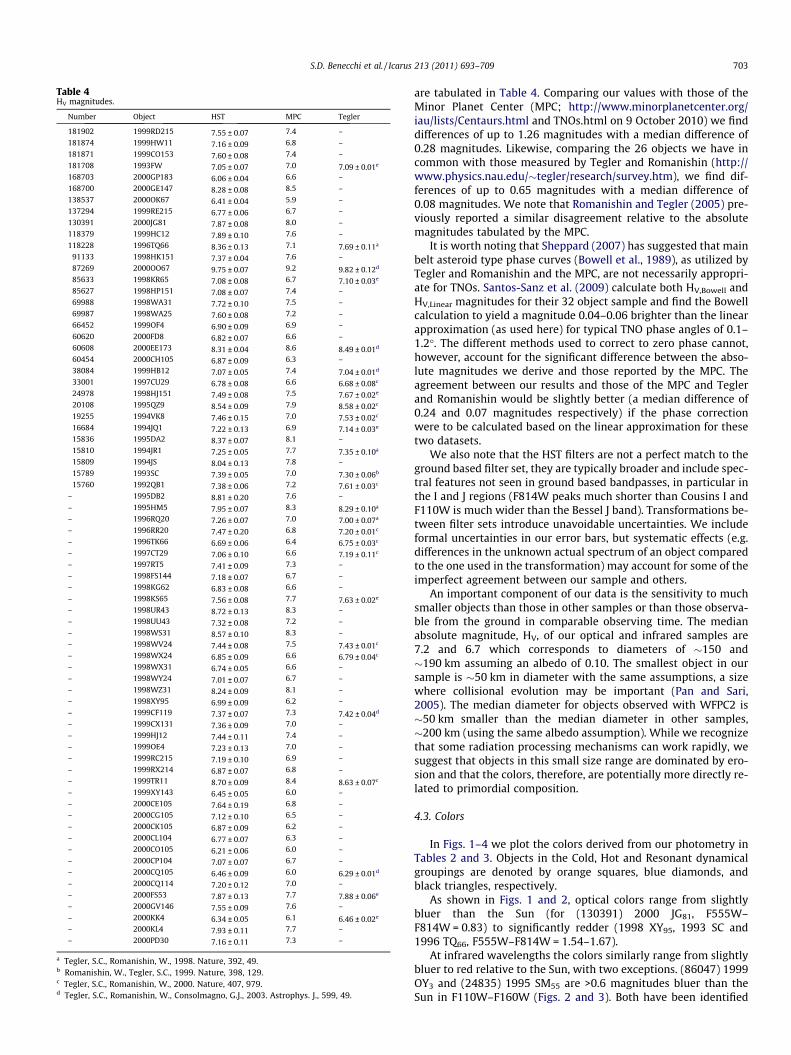
Table 4HV magnitudes.
Number Object HST MPC Tegler
181902 1999RD215 7.55 ± 0.07 7.4 –
181874 1999HW11 7.16 ± 0.09 6.8 –
181871 1999CO153 7.60 ± 0.08 7.4 –
181708 1993FW 7.05 ± 0.07 7.0 7.09 ± 0.01e
168703 2000GP183 6.06 ± 0.04 6.6 –
168700 2000GE147 8.28 ± 0.08 8.5 –
138537 2000OK67 6.41 ± 0.04 5.9 –
137294 1999RE215 6.77 ± 0.06 6.7 –
130391 2000JG81 7.87 ± 0.08 8.0 –
118379 1999HC12 7.89 ± 0.10 7.6 –
118228 1996TQ66 8.36 ± 0.13 7.1 7.69 ± 0.11a
91133 1998HK151 7.37 ± 0.04 7.6 –
87269 2000OO67 9.75 ± 0.07 9.2 9.82 ± 0.12d
85633 1998KR65 7.08 ± 0.08 6.7 7.10 ± 0.03e
85627 1998HP151 7.08 ± 0.07 7.4 –
69988 1998WA31 7.72 ± 0.10 7.5 –
69987 1998WA25 7.60 ± 0.08 7.2 –
66452 1999OF4 6.90 ± 0.09 6.9 –
60620 2000FD8 6.82 ± 0.07 6.6 –
60608 2000EE173 8.31 ± 0.04 8.6 8.49 ± 0.01d
60454 2000CH105 6.87 ± 0.09 6.3 –
38084 1999HB12 7.07 ± 0.05 7.4 7.04 ± 0.01d
33001 1997CU29 6.78 ± 0.08 6.6 6.68 ± 0.08c
24978 1998HJ151 7.49 ± 0.08 7.5 7.67 ± 0.02e
20108 1995QZ9 8.54 ± 0.09 7.9 8.58 ± 0.02c
19255 1994VK8 7.46 ± 0.15 7.0 7.53 ± 0.02c
16684 1994JQ1 7.22 ± 0.13 6.9 7.14 ± 0.03e
15836 1995DA2 8.37 ± 0.07 8.1 –
15810 1994JR1 7.25 ± 0.05 7.7 7.35 ± 0.10a
15809 1994JS 8.04 ± 0.13 7.8 –
15789 1993SC 7.39 ± 0.05 7.0 7.30 ± 0.06b
15760 1992QB1 7.38 ± 0.06 7.2 7.61 ± 0.03c
– 1995DB2 8.81 ± 0.20 7.6 –
– 1995HM5 7.95 ± 0.07 8.3 8.29 ± 0.10a
– 1996RQ20 7.26 ± 0.07 7.0 7.00 ± 0.07a
– 1996RR20 7.47 ± 0.20 6.8 7.20 ± 0.01c
– 1996TK66 6.69 ± 0.06 6.4 6.75 ± 0.03c
– 1997CT29 7.06 ± 0.10 6.6 7.19 ± 0.11c
– 1997RT5 7.41 ± 0.09 7.3 –
– 1998FS144 7.18 ± 0.07 6.7 –
– 1998KG62 6.83 ± 0.08 6.6 –
– 1998KS65 7.56 ± 0.08 7.7 7.63 ± 0.02e
– 1998UR43 8.72 ± 0.13 8.3 –
– 1998UU43 7.32 ± 0.08 7.2 –
– 1998WS31 8.57 ± 0.10 8.3 –
– 1998WV24 7.44 ± 0.08 7.5 7.43 ± 0.01c
– 1998WX24 6.85 ± 0.09 6.6 6.79 ± 0.04c
– 1998WX31 6.74 ± 0.05 6.6 –
– 1998WY24 7.01 ± 0.07 6.7 –
– 1998WZ31 8.24 ± 0.09 8.1 –
– 1998XY95 6.99 ± 0.09 6.2 –
– 1999CF119 7.37 ± 0.07 7.3 7.42 ± 0.04d
– 1999CX131 7.36 ± 0.09 7.0 –
– 1999HJ12 7.44 ± 0.11 7.4 –
– 1999OE4 7.23 ± 0.13 7.0 –
– 1999RC215 7.19 ± 0.10 6.9 –
– 1999RX214 6.87 ± 0.07 6.8 –
– 1999TR11 8.70 ± 0.09 8.4 8.63 ± 0.07c
– 1999XY143 6.45 ± 0.05 6.0 –
– 2000CE105 7.64 ± 0.19 6.8 –
– 2000CG105 7.12 ± 0.10 6.5 –
– 2000CK105 6.87 ± 0.09 6.2 –
– 2000CL104 6.77 ± 0.07 6.3 –
– 2000CO105 6.21 ± 0.06 6.0 –
– 2000CP104 7.07 ± 0.07 6.7 –
– 2000CQ105 6.46 ± 0.09 6.0 6.29 ± 0.01d
– 2000CQ114 7.20 ± 0.12 7.0 –
– 2000FS53 7.87 ± 0.13 7.7 7.88 ± 0.06e
– 2000GV146 7.55 ± 0.09 7.6 –
– 2000KK4 6.34 ± 0.05 6.1 6.46 ± 0.02e
– 2000KL4 7.93 ± 0.11 7.7 –
– 2000PD30 7.16 ± 0.11 7.3 –
a Tegler, S.C., Romanishin, W., 1998. Nature, 392, 49.b Romanishin, W., Tegler, S.C., 1999. Nature, 398, 129.c Tegler, S.C., Romanishin, W., 2000. Nature, 407, 979.d Tegler, S.C., Romanishin, W., Consolmagno, G.J., 2003. Astrophys. J., 599, 49.
S.D. Benecchi et al. / Icarus 213 (2011) 693–709 703
are tabulated in Table 4. Comparing our values with those of theMinor Planet Center (MPC; http://www.minorplanetcenter.org/iau/lists/Centaurs.html and TNOs.html on 9 October 2010) we finddifferences of up to 1.26 magnitudes with a median difference of0.28 magnitudes. Likewise, comparing the 26 objects we have incommon with those measured by Tegler and Romanishin (http://www.physics.nau.edu/�tegler/research/survey.htm), we find dif-ferences of up to 0.65 magnitudes with a median difference of0.08 magnitudes. We note that Romanishin and Tegler (2005) pre-viously reported a similar disagreement relative to the absolutemagnitudes tabulated by the MPC.
It is worth noting that Sheppard (2007) has suggested that mainbelt asteroid type phase curves (Bowell et al., 1989), as utilized byTegler and Romanishin and the MPC, are not necessarily appropri-ate for TNOs. Santos-Sanz et al. (2009) calculate both HV,Bowell andHV,Linear magnitudes for their 32 object sample and find the Bowellcalculation to yield a magnitude 0.04–0.06 brighter than the linearapproximation (as used here) for typical TNO phase angles of 0.1–1.2�. The different methods used to correct to zero phase cannot,however, account for the significant difference between the abso-lute magnitudes we derive and those reported by the MPC. Theagreement between our results and those of the MPC and Teglerand Romanishin would be slightly better (a median difference of0.24 and 0.07 magnitudes respectively) if the phase correctionwere to be calculated based on the linear approximation for thesetwo datasets.
We also note that the HST filters are not a perfect match to theground based filter set, they are typically broader and include spec-tral features not seen in ground based bandpasses, in particular inthe I and J regions (F814W peaks much shorter than Cousins I andF110W is much wider than the Bessel J band). Transformations be-tween filter sets introduce unavoidable uncertainties. We includeformal uncertainties in our error bars, but systematic effects (e.g.differences in the unknown actual spectrum of an object comparedto the one used in the transformation) may account for some of theimperfect agreement between our sample and others.
An important component of our data is the sensitivity to muchsmaller objects than those in other samples or than those observa-ble from the ground in comparable observing time. The medianabsolute magnitude, HV, of our optical and infrared samples are7.2 and 6.7 which corresponds to diameters of �150 and�190 km assuming an albedo of 0.10. The smallest object in oursample is �50 km in diameter with the same assumptions, a sizewhere collisional evolution may be important (Pan and Sari,2005). The median diameter for objects observed with WFPC2 is�50 km smaller than the median diameter in other samples,�200 km (using the same albedo assumption). While we recognizethat some radiation processing mechanisms can work rapidly, wesuggest that objects in this small size range are dominated by ero-sion and that the colors, therefore, are potentially more directly re-lated to primordial composition.
4.3. Colors
In Figs. 1–4 we plot the colors derived from our photometry inTables 2 and 3. Objects in the Cold, Hot and Resonant dynamicalgroupings are denoted by orange squares, blue diamonds, andblack triangles, respectively.
As shown in Figs. 1 and 2, optical colors range from slightlybluer than the Sun (for (130391) 2000 JG81, F555W–F814W = 0.83) to significantly redder (1998 XY95, 1993 SC and1996 TQ66, F555W–F814W = 1.54–1.67).
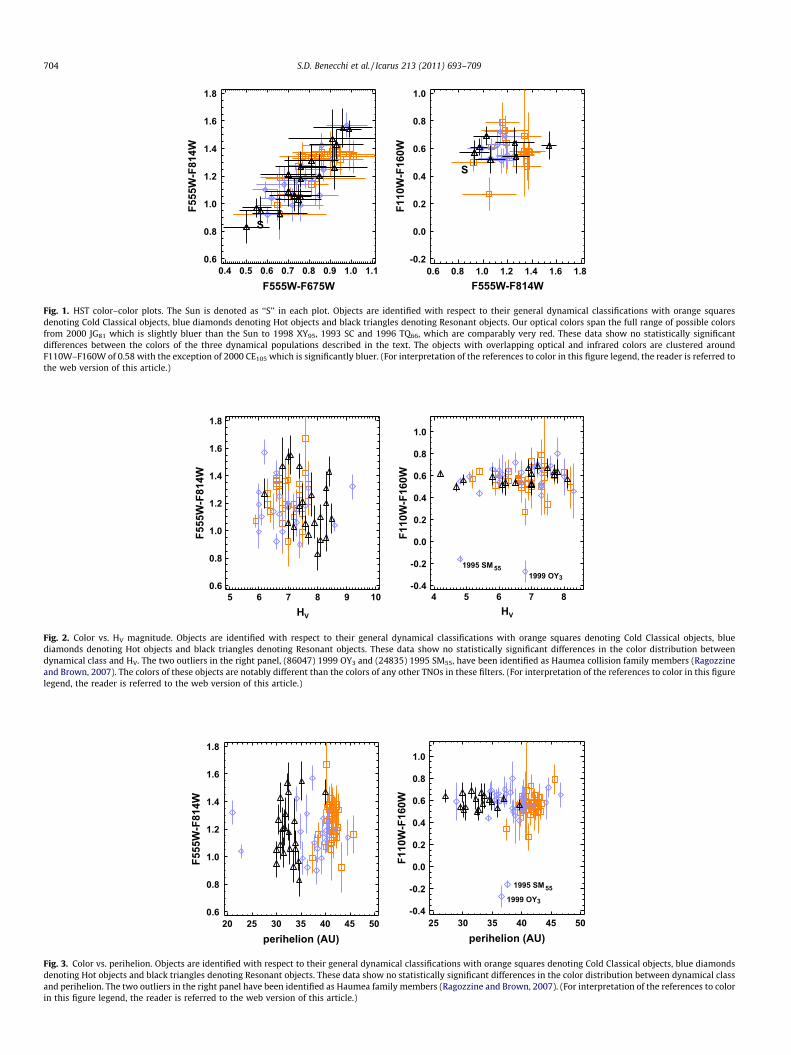
At infrared wavelengths the colors similarly range from slightlybluer to red relative to the Sun, with two exceptions. (86047) 1999OY3 and (24835) 1995 SM55 are >0.6 magnitudes bluer than theSun in F110W–F160W (Figs. 2 and 3). Both have been identified
0.4 0.5 0.6 0.7 0.8 0.9 1.0 1.1F555W-F675W
F555
W-F
814W
S
0.6
0.8
1.0
1.2
1.4
1.6
1.8
0.6 0.8 1.0 1.2 1.4 1.6 1.8F555W-F814W
F110
W-F
160W
S
-0.2
0.0
0.2
0.4
0.6
0.8
1.0
Fig. 1. HST color–color plots. The Sun is denoted as ‘‘S’’ in each plot. Objects are identified with respect to their general dynamical classifications with orange squaresdenoting Cold Classical objects, blue diamonds denoting Hot objects and black triangles denoting Resonant objects. Our optical colors span the full range of possible colorsfrom 2000 JG81 which is slightly bluer than the Sun to 1998 XY95, 1993 SC and 1996 TQ66, which are comparably very red. These data show no statistically significantdifferences between the colors of the three dynamical populations described in the text. The objects with overlapping optical and infrared colors are clustered aroundF110W–F160W of 0.58 with the exception of 2000 CE105 which is significantly bluer. (For interpretation of the references to color in this figure legend, the reader is referred tothe web version of this article.)
5 6 7 8 9 10
F555
W-F
814W
HV
0.6
0.8
1.0
1.2
1.4
1.6
1.8
4 5 6 7 8
F110
W-F
160W
HV
1995 SM 551999 OY3
-0.4
-0.2
0.0
0.2
0.4
0.6
0.8
1.0
Fig. 2. Color vs. HV magnitude. Objects are identified with respect to their general dynamical classifications with orange squares denoting Cold Classical objects, bluediamonds denoting Hot objects and black triangles denoting Resonant objects. These data show no statistically significant differences in the color distribution betweendynamical class and HV. The two outliers in the right panel, (86047) 1999 OY3 and (24835) 1995 SM55, have been identified as Haumea collision family members (Ragozzineand Brown, 2007). The colors of these objects are notably different than the colors of any other TNOs in these filters. (For interpretation of the references to color in this figurelegend, the reader is referred to the web version of this article.)
20 25 30 35 40 45 50perihelion (AU)
F555
W-F
814W
0.6
0.8
1.0
1.2
1.4
1.6
1.8
25 30 35 40 45 50perihelion (AU)
F110
W-F
160W
1995 SM 55
1999 OY3-0.4
-0.2
0.0
0.2
0.4
0.6
0.8
1.0
Fig. 3. Color vs. perihelion. Objects are identified with respect to their general dynamical classifications with orange squares denoting Cold Classical objects, blue diamondsdenoting Hot objects and black triangles denoting Resonant objects. These data show no statistically significant differences in the color distribution between dynamical classand perihelion. The two outliers in the right panel have been identified as Haumea family members (Ragozzine and Brown, 2007). (For interpretation of the references to colorin this figure legend, the reader is referred to the web version of this article.)
704 S.D. Benecchi et al. / Icarus 213 (2011) 693–709
0.2 0.4 0.6 0.8 1.0V-R
V-I
S
0.4
0.6
0.8
1.0
1.2
1.4
1.6
1.8
0.4 0.6 0.8 1.0 1.2 1.4 1.6 1.8V-I
J-H
S
-0.6
-0.4
-0.2
-0.0
0.2
0.4
0.6
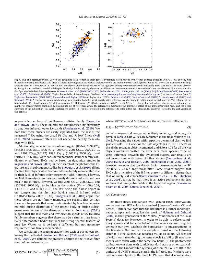
Fig. 4. HST and literature colors. Objects are identified with respect to their general dynamical classifications with orange squares denoting Cold Classical objects, bluediamonds denoting Hot objects and black triangles denoting Resonant objects, literature colors are identified with small symbols while HST colors are identified with largesymbols. The Sun is denoted as ‘‘S’’ in each plot. The objects on the lower left part of the right plot belong to the Haumea collision family. Error bars are on the order of 0.05–0.15 magnitudes and have been left off the plot for clarity. Fundamentally, there are no differences between the quantitative results of these two datasets. Literature colors forthis figure include the following datasets: Doressoundiram et al. (2001, 2005, 2007), Delsanti et al. (2001, 2006), Jewitt and Luu (2001), Trujillo and Brown (2002), Boehnhardtet al. (2002), Peixinho et al. (2004), Tegler, Romanishin, & Consolmagno database (http://www.physics.nau.edu/�tegler/research/survey.htm) inclusive of values from: ?,Tegler and Romanishin (2000, 2003), Romanishin and Tegler (1999) and Tegler et al. (2003), DeMeo et al. (2009), Santos-Sanz et al. (2009), ?), Snodgrass et al. (2010), andSheppard (2010). A copy of our compiled database, incorporating both this work and the cited references can be found in online supplemental material. The columns of thetable include: (1) object number, (2) MPC designation, (3) MPC name, (4) DES classification, (5) MPC HV, (6-23) three columns for each color: color, sigma on color, and thenumber of measurements combined, (24) combined list of references where the reference is defined by the first three letters of the first author’s last name and the 2 yearextension of the publication (this work is referenced as Ben11). (For interpretation of the references to color in this figure legend, the reader is referred to the web version ofthis article.)
S.D. Benecchi et al. / Icarus 213 (2011) 693–709 705
as probable members of the Haumea collision family (Ragozzineand Brown, 2007). These objects are characterized by extremelystrong near infrared water ice bands (Snodgrass et al., 2010). Wenote that these objects are easily separated from the rest of themeasured TNOs using the broad F110W and F160W filters (Nollet al., 2005). Narrower filters are not needed to identify these ob-jects with HST.
Additionally, we note that ten of our targets: (86047) 1999 OY3,(24835) 1995 SM55, 1996 RQ20, 1999 OH4, 2001 QC298, 2000 CG105,and 1999 CD158,(86177) 1999 RY215, (130391) 2000 JG81, and(20161) 1996 TR66, were considered potential Haumea family can-didates or diffused TNOs nearby based on dynamical studies inRagozzine and Brown (2007). In their search of the photometric lit-erature and in subsequent studies by Snodgrass et al. (2010) all butthe first two objects were discounted from family membership dueto their lack of infrared color agreement with Haumea. Likewise,we find these objects to have extremely different colors from Hau-mea in the infrared. However, we find 2001 QC298, 2000CG105, and(130391) 2000 JG81 to be blue in the optical (V–I = 1.00 ± 0.08,1.11 ± 0.13, and 0.80 ± 0.12), the last being the bluest object inour sample and the first also having neutral infrared colors(F110W–F160W = 0.61 ± 0.18). Snodgrass et al. (2010) argue thatthese objects are not family members, we suggest that perhapsthese are fragments that were contaminated by less blue, non-icematerial during disruption of the parent body or during subse-quent re-accretion of the disrupted material. Cook et al. (2011)suggest that the low mass and low ejection speeds of icy Haumeafamily members suggests that there may be a similar mass in par-tially differentiated bodies that lack the strong spectral features ofpure ice. Water ice is perhaps a sufficient but not necessaryrequirement for family membership.
We calculated the spectral gradient for each of our objects fol-lowing the method of Hainaut and Delsanti (2002) and Boehnhardtet al. (2002). We defined the gradient relative to the F555W filter(our defined reference) as:
SðF555W; F814WÞ ¼ 104 RðF814WÞ—RðF555WÞkF814W—kF555W
� �; ð2Þ
where R(F555W) and R(F814W) are the normalized reflectances,
RðkÞ ¼ 10�0:4½ðmk�mref Þ�ðmk;Sun�mref ;SunÞ�; ð3Þ
and mk = mF555W and mF814W, respectively and mk,Sun and mref,Sun aregiven in Table 2. Our values are tabulated in the final column of Ta-ble 2. Averaging the values with respect to dynamical class we findgradients of: 9.35 ± 4.55 for the Cold objects (i < 6�), 8.18 ± 5.89 forthe all the resonant objects combined, and 6.79 ± 4.72 for all the Hotobjects combined. Within the error bars, there appears to be nogreat difference between the dynamical classes. Our results arenot inconsistent with those of other studies (Santos-Sanz et al.,2009; Hainaut and Delsanti, 2002; Boehnhardt et al., 2002, 2003),however, we note that our dataset lacks measurements in the ‘‘B’’(or Blue, k � 4372 angstroms) filter. Some studies suggest thatTNO colors inclusive of the B filter present a different picture thanthat of solely VRI colors (Doressoundiram et al., 2007; Stephenset al., 2003). It may be that there is an active component on TNOsurfaces that is only observable in the B spectral region (Doressoun-diram et al., 2005; Santos-Sanz et al., 2009).
4.4. Comparisons
For more direct comparison with ground-based observationswe convert our HST colors to standard Johnson–Cousins VRI andBessel JH filters. We note that the literature is a rather inhomoge-neous sample and recognize the work of Hainaut and Delsanti(2002) in their generation of the MBOSS (Minor Bodies of the SolarSystem) database. However, in order to be able to reference pri-mary sources and to be confident of the values we are using, wegenerate our own database for comparison to measurements inthe literature. Our comparison sample is based on the followingcriteria: (1) the dataset has reported VRI or JH colors, (2) each setof colors was taken during the same epoch, i.e. VRI or JH measure-ments were taken within the same few hours, (3) the photometriccalibration was done with Landolt standard stars or other stars cal-ibrated to the Landolt filter system (Johnson BV, Cousins RI) in theoptical and UKIRT standard stars in the infrared, and (4) there were�20 or more objects in the sample. We note that it is imperative
706 S.D. Benecchi et al. / Icarus 213 (2011) 693–709
that colors be collected as close in time to each other to minimizelightcurve complications and that the filter network employed forphotometric calibration among different datasets is identical.
Published observations include measurements collected in Bes-sel, Johnson–Cousins and Mould filters. Each one of these filters hasa slightly different response at the wavelengths of interest and inparticular in the R and I bandpasses. Knowing which filter set isused is critical for proper combination of different datasets unlessthe same standard star network (or at least the same filter set) isreferenced by all. Bessel filters have effectively the same bandpass-es in the R and I wavelengths as Cousins filters, however the
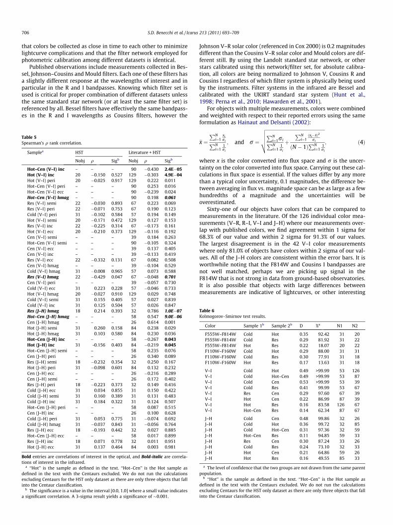
Table 5Spearman’s q rank correlation.
Samplea HST Literature + HST
Nobj q Sigb Nobj q Sigb
Hot–Cen (V–I) inc – – – 90 �0.430 2.4E�05Hot (V–I) inc 20 �0.150 0.527 129 �0.303 4.9E�04Hot (V–I) peri 20 �0.025 0.917 129 0.222 0.011Hot–Cen (V–I) peri – – – 90 0.253 0.016Hot–Cen (V–I) ecc – – – 90 �0.239 0.024Hot–Cen (V–I) hmag – – – 90 0.198 0.061Res (V–I) semi 22 �0.030 0.893 67 0.223 0.069Res (V–I) peri 22 �0.071 0.753 67 0.190 0.123Cold (V–I) peri 31 �0.102 0.584 57 0.194 0.149Hot (V–I) semi 20 �0.171 0.472 129 0.127 0.153Res (V–I) inc 22 �0.225 0.314 67 �0.173 0.161Hot (V–I) ecc 20 �0.210 0.373 129 �0.116 0.192Cen (V–I) semi – – – 39 0.184 0.263Hot–Cen (V–I) semi – – – 90 �0.105 0.324Cen (V–I) ecc – – – 39 0.137 0.405Cen (V–I) inc – – – 39 �0.133 0.419Res (V–I) ecc 22 �0.332 0.131 67 0.082 0.508Cen (V–I) hmag – – – 39 �0.104 0.529Cold (V–I) hmag 31 �0.008 0.965 57 0.073 0.588Res (V–I) hmag 22 �0.429 0.047 67 �0.048 0.701Cen (V–I) peri – – – 39 �0.057 0.730Cold (V–I) ecc 31 0.223 0.228 57 �0.046 0.733Hot (V–I) hmag 20 �0.027 0.910 129 0.029 0.748Cold (V–I) semi 31 0.155 0.405 57 0.027 0.839Cold (V–I) inc 31 0.125 0.504 57 0.026 0.847Res (J–H) hmag 18 0.214 0.393 32 0.786 1.0E�07Hot–Cen (J–H) hmag – – – 58 0.547 9.0E�06Cen (J–H) hmag – – – 26 0.614 0.001Hot (J–H) semi 31 0.260 0.158 84 0.238 0.029Hot (J–H) hmag 31 0.103 0.580 84 0.230 0.036Hot–Cen (J–H) inc – – – 58 �0.267 0.043Hot (J–H) inc 31 -0.156 0.403 84 �0.219 0.045Hot–Cen (J–H) semi – – – 58 0.235 0.076Cen (J–H) peri – – – 26 0.340 0.089Res (J–H) semi 18 �0.232 0.354 32 0.250 0.167Hot (J–H) peri 31 �0.098 0.601 84 0.132 0.232Cen (J–H) ecc – – – 26 �0.216 0.289Cen (J–H) semi – – – 26 0.172 0.402Res (J–H) peri 18 �0.223 0.373 32 0.149 0.416Cold (J–H) ecc 31 0.034 0.855 31 0.150 0.422Cold (J–H) semi 31 0.160 0.389 31 0.131 0.483Cold (J–H) inc 31 0.184 0.322 31 0.124 0.507Hot–Cen (J–H) peri – – – 58 0.087 0.515Cen (J–H) inc – – – 26 0.100 0.628Cold (J–H) peri 31 0.053 0.775 31 �0.074 0.692Cold (J–H) hmag 31 �0.037 0.843 31 �0.056 0.764Res (J–H) ecc 18 �0.193 0.442 32 0.027 0.885Hot–Cen (J–H) ecc – – – 58 0.017 0.899Res (J–H) inc 18 0.071 0.778 32 0.011 0.951Hot (J–H) ecc 31 0.137 0.464 84 0.003 0.981
Bold entries are correlations of interest in the optical, and Bold-italic are correla-tions of interest in the infrared.
a ‘‘Hot’’ is the sample as defined in the text. ‘‘Hot–Cen’’ is the Hot sample asdefined in the text with the Centaurs excluded. We do not run the calculationsexcluding Centaurs for the HST only dataset as there are only three objects that fallinto the Centaur classification.
b The significance is a value in the interval [0.0, 1.0] where a small value indicatesa significant correlation. A 3-sigma result yields a significance of �0.001.
Johnson V–R solar color (referenced in Cox 2000) is 0.2 magnitudesdifferent than the Cousins V–R solar color and Mould colors are dif-ferent still. By using the Landolt standard star network, or otherstars calibrated using this network/filter set, for absolute calibra-tion, all colors are being normalized to Johnson V, Cousins R andCousins I regardless of which filter system is physically being usedby the instruments. Filter systems in the infrared are Bessel andcalibrated with the UKIRT standard star system (Hunt et al.,1998; Perna et al., 2010; Hawarden et al., 2001).
For objects with multiple measurements, colors were combinedand weighted with respect to their reported errors using the sameformulation as Hainaut and Delsanti (2002):
�x ¼PN
i¼1xiriPN
i¼11ri
; and r ¼
ffiffiffiffiffiffiffiffiffiffiffiffiffiffiffiffiffiffiffiffiffiffiffiffiffiffiffiffiffiffiffiffiffiffiffiffiffiffiffiffiffiffiffiffiffiffiffiffiffiffiffiPNi¼1riPNi¼1
1ri
þPN
i¼1ðxi��xÞ2
ri
ðN � 1ÞPN
i¼11ri
vuuut ; ð4Þ
where x is the color converted into flux space and r is the uncer-tainty on the color converted into flux space. Carrying out these cal-culations in flux space is essential. If the values differ by any morethan a typical color uncertainty, 0.1 magnitudes, the difference be-tween averaging in flux vs. magnitude space can be as large as a fewhundredths of a magnitude and the uncertainties will beoverestimated.
Sixty-one of our objects have colors that can be compared tomeasurements in the literature. Of the 126 individual color mea-surements (V–R, R–I, V–I and J–H) where our measurements over-lap with published colors, we find agreement within 1 sigma for68.3% of our value and within 2 sigma for 91.3% of our values.The largest disagreement is in the 42 V–I color measurementswhere only 81.0% of objects have colors within 2 sigma of our val-ues. All of the J–H colors are consistent within the error bars. It isworthwhile noting that the F814W and Cousins I bandpasses arenot well matched, perhaps we are picking up signal in theF814W that is not strong in data from ground-based observatories.It is also possible that objects with large differences betweenmeasurements are indicative of lightcurves, or other interesting
Table 6Kolmogorov–Smirnov test results.
Color Sample 1b Sample 2b D %a N1 N2
F555W–F814W Cold Hot 0.35 92.42 31 20F555W–F814W Cold Res 0.29 81.92 31 22F555W–F814W Hot Res 0.22 18.07 20 22F110W–F160W Cold Hot 0.29 88.00 31 31F110W–F160W Cold Res 0.30 77.91 31 18F110W–F160W Hot Res 0.17 13.63 31 18
V–I Cold Hot 0.49 >99.99 53 126V–I Cold Hot–Cen 0.49 >99.99 53 87V–I Cold Cen 0.53 >99.99 53 39V–I Cold Res 0.41 99.99 53 67V–I Res Cen 0.29 97.60 67 39V–I Hot Cen 0.22 86.99 87 39V–I Hot Res 0.16 83.58 126 67V–I Hot–Cen Res 0.14 62.34 87 67
J–H Cold Cen 0.48 99.86 32 26J–H Cold Hot 0.36 99.72 32 85J–H Cold Hot–Cen 0.31 97.36 32 59J–H Hot–Cen Res 0.11 94.85 59 33J–H Res Cen 0.30 87.24 33 26J–H Cold Res 0.24 73.10 32 33J–H Hot Cen 0.21 64.86 59 26J–H Hot Res 0.16 49.55 85 33
a The level of confidence that the two groups are not drawn from the same parentpopulation.
b ‘‘Hot’’ is the sample as defined in the text. ‘‘Hot–Cen’’ is the Hot sample asdefined in the text with the Centaurs excluded. We do not run the calculationsexcluding Centaurs for the HST only dataset as there are only three objects that fallinto the Centaur classification.
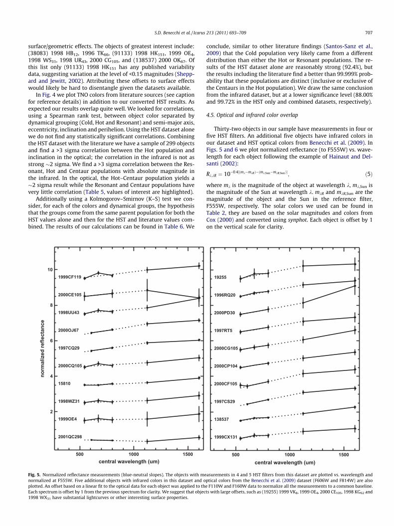
S.D. Benecchi et al. / Icarus 213 (2011) 693–709 707
surface/geometric effects. The objects of greatest interest include:(38083) 1998 HB12, 1996 TK66, (91133) 1998 HK151, 1999 OE4,1998 WS31, 1998 UR43, 2000 CG105, and (138537) 2000 OK67. Ofthis list only (91133) 1998 HK151 has any published variabilitydata, suggesting variation at the level of <0.15 magnitudes (Shepp-ard and Jewitt, 2002). Attributing these offsets to surface effectswould likely be hard to disentangle given the datasets available.
In Fig. 4 we plot TNO colors from literature sources (see captionfor reference details) in addition to our converted HST results. Asexpected our results overlap quite well. We looked for correlations,using a Spearman rank test, between object color separated bydynamical grouping (Cold, Hot and Resonant) and semi-major axis,eccentricity, inclination and perihelion. Using the HST dataset alonewe do not find any statistically significant correlations. Combiningthe HST dataset with the literature we have a sample of 299 objectsand find a >3 sigma correlation between the Hot population andinclination in the optical; the correlation in the infrared is not asstrong �2 sigma. We find a >3 sigma correlation between the Res-onant, Hot and Centaur populations with absolute magnitude inthe infrared. In the optical, the Hot–Centaur population yields a�2 sigma result while the Resonant and Centaur populations havevery little correlation (Table 5, values of interest are highlighted).
Additionally using a Kolmogorov–Smirnov (K–S) test we con-sider, for each of the colors and dynamical groups, the hypothesisthat the groups come from the same parent population for both theHST values alone and then for the HST and literature values com-bined. The results of our calculations can be found in Table 6. We
500 1000 1500central wavelength (um)
norm
aliz
ed re
flect
ance
2001QC298
1999OE4
1998WZ31
15810
2000CQ105
1997CQ29
2000OJ67
1998UU43
2000CE105
1999CF119
2
4
6
8
10
Fig. 5. Normalized reflectance measurements (blue-neutral slopes). The objects with menormalized at F555W. Five additional objects with infrared colors in this dataset and oplotted. An offset based on a linear fit to the optical data for each object was applied to thEach spectrum is offset by 1 from the previous spectrum for clarity. We suggest that objec1998 WX31 have substantial lightcurves or other interesting surface properties.
conclude, similar to other literature findings (Santos-Sanz et al.,2009) that the Cold population very likely came from a differentdistribution than either the Hot or Resonant populations. The re-sults of the HST dataset alone are reasonably strong (92.4%), butthe results including the literature find a better than 99.999% prob-ability that these populations are distinct (inclusive or exclusive ofthe Centaurs in the Hot population). We draw the same conclusionfrom the infrared dataset, but at a lower significance level (88.00%and 99.72% in the HST only and combined datasets, respectively).
4.5. Optical and infrared color overlap
Thirty-two objects in our sample have measurements in four orfive HST filters. An additional five objects have infrared colors inour dataset and HST optical colors from Benecchi et al. (2009). InFigs. 5 and 6 we plot normalized reflectance (to F555W) vs. wave-length for each object following the example of Hainaut and Del-santi (2002):
Rk;kR ¼ 10�0:4½ðmk�mkRÞ�ðmk;Sun�mkR;SunÞ�; ð5Þ
where mk is the magnitude of the object at wavelength k, mk,Sun isthe magnitude of the Sun at wavelength k. mkR and mkR,Sun are themagnitude of the object and the Sun in the reference filter,F555W, respectively. The solar colors we used can be found inTable 2, they are based on the solar magnitudes and colors fromCox (2000) and converted using synphot. Each object is offset by 1on the vertical scale for clarity.
500 1000 1500central wavelength (um)
1999CX131
138537
1997CS29
2000CF105
2000CP104
2000CG105
1997RT5
2000PD30
1996RQ20
19255
asurements in 4 and 5 HST filters from this dataset are plotted vs. wavelength andptical colors from the Benecchi et al. (2009) dataset (F606W and F814W) are alsoe F110W and F160W data to normalize all the measurements to a common baseline.ts with large offsets, such as (19255) 1999 VK8, 1999 OE4, 2000 CE105, 1998 KG62 and
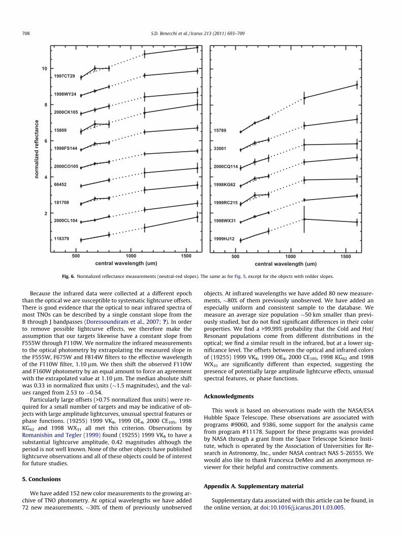
118379
2000CL104
181708
66452
2000CO105
1998FS144
15809
2000CK105
1998WY24
1997CT29
1999HJ12
1998WX31
1999RC215
1998KG62
2000CQ114
33001
15789
norm
aliz
ed re
flect
ance
2
4
6
8
10
500 1000 1500central wavelength (um)
500 1000 1500central wavelength (um)
Fig. 6. Normalized reflectance measurements (neutral-red slopes). The same as for Fig. 5, except for the objects with redder slopes.
708 S.D. Benecchi et al. / Icarus 213 (2011) 693–709
Because the infrared data were collected at a different epochthan the optical we are susceptible to systematic lightcurve offsets.There is good evidence that the optical to near infrared spectra ofmost TNOs can be described by a single constant slope from theB through J bandpasses (Doressoundiram et al., 2007; ?). In orderto remove possible lightcurve effects, we therefore make theassumption that our targets likewise have a constant slope fromF555W through F110W. We normalize the infrared measurementsto the optical photometry by extrapolating the measured slope inthe F555W, F675W and F814W filters to the effective wavelengthof the F110W filter, 1.10 lm. We then shift the observed F110Wand F160W photometry by an equal amount to force an agreementwith the extrapolated value at 1.10 lm. The median absolute shiftwas 0.33 in normalized flux units (�1.5 magnitudes), and the val-ues ranged from 2.53 to �0.54.
Particularly large offsets (>0.75 normalized flux units) were re-quired for a small number of targets and may be indicative of ob-jects with large amplitude lightcurves, unusual spectral features orphase functions. (19255) 1999 VK8, 1999 OE4, 2000 CE105, 1998KG62 and 1998 WX31 all met this criterion. Observations byRomanishin and Tegler (1999) found (19255) 1999 VK8 to have asubstantial lightcurve amplitude, 0.42 magnitudes although theperiod is not well known. None of the other objects have publishedlightcurve observations and all of these objects could be of interestfor future studies.
5. Conclusions
We have added 152 new color measurements to the growing ar-chive of TNO photometry. At optical wavelengths we have added72 new measurements, �30% of them of previously unobserved
objects. At infrared wavelengths we have added 80 new measure-ments, �80% of them previously unobserved. We have added anespecially uniform and consistent sample to the database. Wemeasure an average size population �50 km smaller than previ-ously studied, but do not find significant differences in their colorproperties. We find a >99.99% probability that the Cold and Hot/Resonant populations come from different distributions in theoptical; we find a similar result in the infrared, but at a lower sig-nificance level. The offsets between the optical and infrared colorsof (19255) 1999 VK8, 1999 OE4, 2000 CE105, 1998 KG62 and 1998WX31 are significantly different than expected, suggesting thepresence of potentially large amplitude lightcurve effects, unusualspectral features, or phase functions.
Acknowledgments
This work is based on observations made with the NASA/ESAHubble Space Telescope. These observations are associated withprograms #9060, and 9386, some support for the analysis camefrom program #11178. Support for these programs was providedby NASA through a grant from the Space Telescope Science Insti-tute, which is operated by the Association of Universities for Re-search in Astronomy, Inc., under NASA contract NAS 5-26555. Wewould also like to thank Francesca DeMeo and an anonymous re-viewer for their helpful and constructive comments.
Appendix A. Supplementary material
Supplementary data associated with this article can be found, inthe online version, at doi:10.1016/j.icarus.2011.03.005.
S.D. Benecchi et al. / Icarus 213 (2011) 693–709 709
References
Anderson, J., King, I.R., 1999. Astrometric and photometric corrections for the 34throw error in HST’s WFPC2 camera. Publ. Astron. Soc. Pacific 111, 1095–1098.
Baggett, S. et al., 2002. In: Mobasher, B. (Ed.), HST WFPC2 Data Handbook, Version4.0. STScI, Baltimore. <http://www.stsci.edu/hst/wfpc2/Wfpc2_dhb/WFPC2_longdhbcover.html>.
Benecchi, S.D., Noll, K.S., Grundy, W.M., Buie, M.W., Stephens, D.C., Levison, H.F.,2009. The correlated colors of transneptunian binaries. Icarus 200, 292–303.
Boehnhardt et al., 2002. ESO large program on physical studies of transneptunianobjects and Centaurs: Visible photometry – First results. Astron. Astrophys. 395,297–303.
Boehnhardt et al., 2003. Results from the ESO large program on transneptunianobjects and Centaurs. Earth 92, 145–156.
Bowell, E., Hapke, E.B., Domingue, D., Lumme, K., Peltoniemi, J., Harris, A.W., 1989.Application of photometric models to asteroids. In: Binzel, R.P., Gehrels, R.,Matthews, M.S. (Eds.), Asteroids II. Univ. of Arizona Press, Tucson, pp. 524–556.
Brucker, M.J., Grundy, W.M., Stansberry, J.A., Spencer, J.R., Sheppard, S.S., Chiang, E.I.,Buie, M.W., 2009. High albedos of low inclination Classical Kuiper belt objects.Icarus 201, 284–294.
Cook, J.C., Desch, S.J., Rubin, M. 2011. The black sheep of Haumea’s collisionalfamily. Lunar Planet. Sci. 42, 2503.
Cox, A.N., 2000. Allen’s Astrophysical Quantities. Springer, New York. pp. 341.Delsanti, A.C., Peixinho, N., Boehnhardt, H., Barucci, M.A., Merlin, F.,
Doressoundiram, A., Davies, J.K., 2006. Near-Infrared Color Properties ofKuiper Belt Objects and Centaurs: Final Results from the ESO Large Program.The Astronomical Journal 131, 1851–1863.
de Jong, R.S., 2006. Correcting the NICMOS count-rate dependent non-linearity.Instrument Science Report NICMOS 2006-003, 3-14.
Delsanti, A.C., Boehnhardt, H., Barrera, L., Meech, K.J., Sekiguchi, T., Hainaut, O.R.,2001. BVRI photometry of 27 Kuiper belt objects with ESO/very large telescope.Astron. Astrophys. 380, 347–358.
DeMeo, F.E., Fornasier, S., Barucci, M.A., Perna, D., Protopapa, S., Alvarez-Candal, A.,Delsanti, A.C., Doressoundiram, A., Merlin, F., de Bergh, C., 2009. Visible andnear-infrared colors of transneptunian objects and Centaurs from the secondESO large program. Astron. Astrophys. 493, 283–290.
Dolphin, A.E., 2000. The charge-transfer efficiency and calibration of WFPC2. Publ.Astron. Soc. Pacific 112, 1397–1410.
Dolphin, A.E., 2009. A revised characterization of the WFPC2 CTE loss. Publ. Astron.Soc. Pacific 121, 655–667.
Doressoundiram, A., Barucci, M.A., Romon, J., Veillet, C., 2001. Multicolorphotometry of trans-neptunian objects. Icarus 154, 277–286.
Doressoundiram, A., Peixinho, N., Doucet, C., Mousis, O., Barucci, M.A., Petit, J.M.,Veillet, C., 2005. The Meudon Multicolor Survey (2MS) of Centaurs and trans-neptunian objects: extended dataset and status on the correlations reported.Icarus 174, 90–104.
Doressoundiram, A., Peixinho, N., Moullet, A., Fornasier, S., Barucci, M.A., Beuzit, J.-L., Veillet, C., 2007. The Meudon Multicolor Survey (2MS) of Centaurs and Trans-Neptunian Objects: From Visible to Infrared Colors. The Astronomical Journal134, 2186–2199.
Doressoundiram, A., Boehnhardt, H., Tegler, S.C., Trujillo, C., 2008. Color propertiesand trends of the transneptunian objects. In: Barucci, M.A., Boehnhardt, H.,Cruikshank, D.P., Morbidelli, A. (Eds.), The Solar System Beyond Neptune. Univ.of Arizona Press, Tucson, pp. 91–104.
Dressel, L. et al., 2007. STIS Data Handbook, Version 5.0. STScI, Baltimore. <http://www.stsci.edu/hst/stis/documents/handbooks/currentDHB/STIS_longdhbcover.html>.
Elliot, J.L., et al., 2005. The deep ecliptic survey: A search for Kuiper belt objects andCentaurs. II. Dynamical classification, the Kuiper belt plane, and the corepopulation. Astron. J. 129, 1117–1162.
Fernie, 1983. Relationships between the Johnson and Kron–Cousins VRIphotometric systems. Astron. Soc. Pacific 95, 782–785.
Gladman, B., Marsden, B.G., Vanlaerhoven, C., 2008. Nomenclature in the outer solarsystem. In: Barucci, M.A., Boehnhardt, H., Cruikshank, D.P., Morbidelli, A., (Eds.),The Solar System Beyond Neptune. Univ. of Arizona Press, Tucson, pp. 43.
Gomes, R.S., Levison, H.F., Tsiganis, K., Morbidelli, A., 2005. Origin of the cataclysmicLate Heavy Bombardment period of the terrestrial planets. Nature 435, 466–469.
Gulbis, A.A.S., Elliot, J.L., Kane, J.F., 2006. The color of the Kuiper belt core. Icarus 183,168–178.
Hainaut, O.R., Delsanti, A.C., 2002. Colors of minor bodies in the outer Solar System.A statistical analysis. Astron. Astrophys. 389, 641–664.
Hawarden, T.G., Leggett, S.K., Letawsky, M.B., Ballantyne, D.R., Casali, M.M., 2001.JHK standard stars for large telescopes: The UKIRT fundamental and extendedlists. Monthly Notices Roy. Astron. Soc. 325, 563–574.
Howell, S.B., Koehn, B., Bowell, E., Hoffman, M., 1996. Detection and measurementof poorly sampled point sources imaged with 2-D array. Astron. J. 112, 1302–1311.
Hunt, L.K., Mannucci, F., Testi, L., Migliorini, S., Stanga, R.M., Baffa, C., Lisi, F., Vanzi,L., 1998. Northern JHK Standard Stars for Array Detectors. The AstronomicalJournal 115, 2594–2603.
Jewitt, D., Luu, J., 2001. Colors and spectra of Kuiper belt objects. Astron. J. 122,2099–2114.
Krist, J., Hook R. 2004. The Tiny Tim User’s Guide, Version 6.3. STScI, Baltimore.Levison, H.F., Morbidelli, A., Vanlaerhoven, C., Gomes, R.S., Tsiganis, K., 2008. Origin
of the structure of the Kuiper belt during a dynamical instability in the orbits ofUranus and Neptune. Icarus 196, 258–273.
McMaster, Biretta, et al. 2008, WFPC2 Instrument Handbook, Version 10.0. STScI,Baltimore.
Morbidelli, A., Levison, H.F., Tsiganis, K., Gomes, R.S., 2005. Chaotic capture ofJupiter’s Trojan asteroids in the early Solar System. Nature 435, 462–465.
Noll, K., Stephens, D., Grundy, W., Cruikshank, D., Romanishin, W., Tegler, S., 2005.Infrared photometry of Kuiper belt objects with NICMOS. Am. Astron. Soc. 37,746.
Noll, K.S., Grundy, W.M., Stephens, D.C., Levison, H.F., Kern, S.D., 2008. Evidence fortwo populations of classical transneptunian objects: The strong inclinationdependence of classical binaries. Icarus 194, 758–768.
Pan, M., Sari, R., 2005. Shaping the Kuiper belt size distribution by shattering largebut strengthless bodies. Icarus 173, 342–348.
Pavlovsky, C. 2006. ACS Data Handbook, Version 5.0. STScI, Baltimore.Peixinho, N., Doressoundiram, A., Delsanti, A.C., Boehnhardt, H., Barucci, M.A.,
Belskaya, I.N., 2003. Reopening the TNOs color controversy: Centaursbimodality and TNOs unimodality. Astron. Astrophys. 410, 29–32.
Peixinho, N., Boehnhardt, H., Belskaya, I.N., Doressoundiram, A., Barucci, M.A.,Delsanti, A.C., 2004. ESO large program on Centaurs and TNOs: Visible colors-final results. Icarus 170, 153–166.
Peixinho, N., Lacerda, P., Jewitt, D.C., 2008. Relation of the classical Kuiper beltobjects. Astron. J. 136, 1837–1845.
Perna, D., Barucci, M.A., Fornasier, S., DeMeo, F.E., Alvarez-Candal, A., Merlin,Frèdèric, D.E., Doressoundiram, A., de Bergh, C., 2010. Colors and taxonomy ofCentaurs and trans-Neptunian objects. Astronomy and Astrophysics 510, 53–59.
Ragozzine, D., Brown, M., 2007. Candidate members and age estimate of the familyof Kuiper belt object 2003 EL61. Astron. J. 134, 2160–2167.
Romanishin, W.J., Tegler, S.C., 1999. Rotation rates of Kuiper-belt objects from theirlight curves. Nature 398, 129–132.
Romanishin, W.J., Tegler, S.C., 2005. Accurate absolute magnitudes for Kuiper beltobjects and Centaurs. Icarus 179, 523–526.
Romanishin, W.J., Tegler, S.C., Consolmagno, G.J., 2010. Colors of inner disk classicalKuiper belt objects. Astron. J. 140, 29–33.
Santos-Sanz, P., Ortiz, J.L., Barrera, L., Boehnhardt, H., 2009. New BVRI photometryresults on Kuiper belt objects from the ESO VLT. Astron. Astrophys. 494, 693–706.
Sheppard, S.S., 2007. Light curves of dwarf Plutonian planets and other large Kuiperbelt objects: Their rotations, phase functions, and absolute magnitudes. Astron.J. 134, 787–798.
Sheppard, S.S., 2010. The colors of extreme outer Solar System objects. Astron. J.139, 1394–1405.
Sheppard, S.S., Jewitt, D., 2002. Time-resolved photometry of Kuiper belt objects:Rotations, shapes, and phase functions. Astron. J. 124, 1757–1775.
Snodgrass, C., Carry, B., Dumas, C., Hainaut, O.R., 2010. Characterisation of candidatemembers of (136108) Haumea’s family. Astron. Astrophys. 511, A72.
Stephens, D.C., Noll, K.S., 2006. Detection of six trans-neptunian binaries withNICMOS: A high fraction of binaries in the cold classical disk. Astron. J. 131,1142–1148.
Stephens, D.C., Noll, K.S., Grundy, W.M., Millis, R.L., Spencer, J.R., Buie, M.W., Tegler,S.C., Romanishin, W.J., Cruikshank, D.P., 2003. HST Photometry ofTransneptunian Objects. Earth, Moon and Planets 92, 251–260.
Tegler, S.C., Romanishin, W.J., 2000. Extremely red Kuiper-belt objects in near-circular orbits beyond 40 AU. Nature 407, 979–981.
Tegler, S.C., Romanishin, W.J., 2003. Resolution of the Kuiper belt object colorcontroversy: Two distinct color populations. Icarus 161, 181–191.
Tegler, S.C., Romanishin, W.J., Consolmagno, G.J., 2003. Color patterns in the Kuiperbelt: A possible primordial origin. Astrophys. J. 599, 49–52.
Tegler, S.C., Bauer, J.M., Romanishin, W., Peixinho, N., 2008. Colors of Centaurs. In:Barucci, M.A., Boehnhardt, H., Cruikshank, D.P., Morbidelli, A. (Eds.), The SolarSystem Beyond Neptune. Univ. of Arizona Press, Tucson, pp. 105–114.
Thatte, D., Dahlen, T., et al., 2009. NICMOS Data Handbook, Version 8.0. STScI,Baltimore. <http://www.stsci.edu/hst/nicmos/documents/handbooks/DataHandbookv8/>.
Trujillo, C., Brown, M.E., 2002. A correlation between inclination and color in theclassical Kuiper belt. Astrophys. J. 566, 125–128.
Tsiganis, K., Gomes, R.S., Morbidelli, A., Levison, H.F., 2005. Origin of the orbitalarchitecture of the giant planets of the Solar System. Nature 435, 459–461.
Viana, A., Wiklind, T., et al., 2009, NICMOS Instrument Handbook, Version 11.0.STScI, Baltimore. <http://www.stsci.edu/hst/nicmos/documents/handbooks/current_NEW/cover.html>.