Optical-resolution photoacoustic endomicroscopy in vivocoilab.caltech.edu/epub/2015/YangJM_2015_Biomedical Optics Express... · Optical-resolution photoacoustic endomicroscopy in

Optical-resolution photoacoustic endomicroscopy in vivo

Joon-Mo Yang,1,4 Chiye Li,1,4 Ruimin Chen,2,4 Bin Rao,1 Junjie Yao,1 Cheng-Hung Yeh,1 Amos Danielli,1,3 Konstantin Maslov,1 Qifa Zhou,2 K. Kirk Shung,2

and Lihong V. Wang1,* 1 Optical Imaging Laboratory, Department of Biomedical Engineering, Washington University in St. Louis, Campus

Box 1097, One Brookings Drive, St. Louis, Missouri 63130, USA 2NIH Ultrasonic Transducer Resource Center, Department of Biomedical Engineering, University of Southern

California, 1042 Downey Way, University Park, Los Angeles, California 90089, USA 3Currently with the Faculty of Engineering, Bar-Ilan University, Ramat Gan 5290002, Israel

4These authors contributed equally to this work *[email protected]

Abstract: Optical-resolution photoacoustic microscopy (OR-PAM) has become a major experimental tool of photoacoustic tomography, with unique imaging capabilities for various biological applications. However, conventional imaging systems are all table-top embodiments, which preclude their use in internal organs. In this study, by applying the OR-PAM concept to our recently developed endoscopic technique, called photoacoustic endoscopy (PAE), we created an optical-resolution photoacoustic endomicroscopy (OR-PAEM) system, which enables internal organ imaging with a much finer resolution than conventional acoustic-resolution PAE systems. OR-PAEM has potential preclinical and clinical applications using either endogenous or exogenous contrast agents.

©2015 Optical Society of America

OCIS codes: (170.0170) Medical optics and biotechnology; (170.3880) Medical and biological imaging; (170.3890) Medical optics instrumentation; (170.5120) Photoacoustic imaging; (170.2150) Endoscopic imaging; (170.0180) Microscopy.

References and links 1. D. Fukumura, D. G. Duda, L. L. Munn, and R. K. Jain, “Tumor microvasculature and microenvironment: novel

insights through intravital imaging in pre-clinical models,” Microcirculation 17(3), 206–225 (2010). 2. P. Amornphimoltham, A. Masedunskas, and R. Weigert, “Intravital microscopy as a tool to study drug delivery

in preclinical studies,” Adv. Drug Deliv. Rev. 63(1-2), 119–128 (2011). 3. M. R. Fein and M. Egeblad, “Caught in the act: revealing the metastatic process by live imaging,” Dis. Model.

Mech. 6(3), 580–593 (2013). 4. B. J. Vakoc, R. M. Lanning, J. A. Tyrrell, T. P. Padera, L. A. Bartlett, T. Stylianopoulos, L. L. Munn, G. J.

Tearney, D. Fukumura, R. K. Jain, and B. E. Bouma, “Three-dimensional microscopy of the tumor microenvironment in vivo using optical frequency domain imaging,” Nat. Med. 15(10), 1219–1223 (2009).

5. S. H. Yun, G. J. Tearney, B. J. Vakoc, M. Shishkov, W. Y. Oh, A. E. Desjardins, M. J. Suter, R. C. Chan, J. A. Evans, I. K. Jang, N. S. Nishioka, J. F. de Boer, and B. E. Bouma, “Comprehensive volumetric optical microscopy in vivo,” Nat. Med. 12(12), 1429–1433 (2007).

6. M. J. Gora, J. S. Sauk, R. W. Carruth, K. A. Gallagher, M. J. Suter, N. S. Nishioka, L. E. Kava, M. Rosenberg, B. E. Bouma, and G. J. Tearney, “Tethered capsule endomicroscopy enables less invasive imaging of gastrointestinal tract microstructure,” Nat. Med. 19(2), 238–240 (2013).

7. G. M. Tozer, S. M. Ameer-Beg, J. Baker, P. R. Barber, S. A. Hill, R. J. Hodgkiss, R. Locke, V. E. Prise, I. Wilson, and B. Vojnovic, “Intravital imaging of tumour vascular networks using multi-photon fluorescence microscopy,” Adv. Drug Deliv. Rev. 57(1), 135–152 (2005).

8. G. Egawa, S. Nakamizo, Y. Natsuaki, H. Doi, Y. Miyachi, and K. Kabashima, “Intravital analysis of vascular permeability in mice using two-photon microscopy,” Sci. Rep. 3, 1932 (2013).

9. M. G. Velasco and M. J. Levene, “In vivo two-photon microscopy of the hippocampus using glass plugs,” Biomed. Opt. Express 5(6), 1700–1708 (2014).

10. J. Xi, Y. Chen, Y. Zhang, K. Murari, M. J. Li, and X. Li, “Integrated multimodal endomicroscopy platform for simultaneous en face optical coherence and two-photon fluorescence imaging,” Opt. Lett. 37(3), 362–364 (2012).

#229350 - $15.00 USD Received 10 Dec 2014; revised 26 Jan 2015; accepted 28 Jan 2015; published 23 Feb 2015 (C) 2015 OSA 23 Feb 2015 | Vol. 23, No. 4 | DOI:10.1364/OE.23.00918 | OPTICS EXPRESS 918

11. R. Kiesslich, M. Goetz, M. Vieth, P. R. Galle, and M. F. Neurath, “Technology Insight: confocal laser endoscopy for in vivo diagnosis of colorectal cancer,” Nat. Clin. Pract. Oncol. 4(8), 480–490 (2007).

12. Y. Matsumoto, T. Nomoto, H. Cabral, Y. Matsumoto, S. Watanabe, R. J. Christie, K. Miyata, M. Oba, T. Ogura, Y. Yamasaki, N. Nishiyama, T. Yamasoba, and K. Kataoka, “Direct and instantaneous observation of intravenously injected substances using intravital confocal micro-videography,” Biomed. Opt. Express 1(4), 1209–1216 (2010).

13. P. Kim, E. Chung, H. Yamashita, K. E. Hung, A. Mizoguchi, R. Kucherlapati, D. Fukumura, R. K. Jain, and S. H. Yun, “In vivo wide-area cellular imaging by side-view endomicroscopy,” Nat. Methods 7(4), 303–305 (2010).

14. A. A. Oraevsky and A. A. Karabutov, “Optoacoustic Tomography,” in Biomedical Photonics Handbook, T. Vo-Dinh, ed. (CRC Press, New York, 2003).

15. S. Y. Emelianov, P.-C. Li, and M. O’Donnell, “Photoacoustics for molecular imaging and therapy,” Phys. Today 62(5), 34–39 (2009).

16. V. Ntziachristos and D. Razansky, “Molecular imaging by means of multispectral optoacoustic tomography (MSOT),” Chem. Rev. 110(5), 2783–2794 (2010).

17. P. Beard, “Biomedical photoacoustic imaging,” Interface Focus 1(4), 602–631 (2011). 18. L. V. Wang and S. Hu, “Photoacoustic tomography: in vivo imaging from organelles to organs,” Science

335(6075), 1458–1462 (2012). 19. H. F. Zhang, K. Maslov, G. Stoica, and L. V. Wang, “Functional photoacoustic microscopy for high-resolution

and noninvasive in vivo imaging,” Nat. Biotechnol. 24(7), 848–851 (2006). 20. K. Maslov, H. F. Zhang, S. Hu, and L. V. Wang, “Optical-resolution photoacoustic microscopy for in vivo

imaging of single capillaries,” Opt. Lett. 33(9), 929–931 (2008). 21. E. Z. Zhang, B. Povazay, J. Laufer, A. Alex, B. Hofer, B. Pedley, C. Glittenberg, B. Treeby, B. Cox, P. Beard,

and W. Drexler, “Multimodal photoacoustic and optical coherence tomography scanner using an all optical detection scheme for 3D morphological skin imaging,” Biomed. Opt. Express 2(8), 2202–2215 (2011).

22. J. Yao, K. I. Maslov, Y. Zhang, Y. Xia, and L. V. Wang, “Label-free oxygen-metabolic photoacoustic microscopy in vivo,” J. Biomed. Opt. 16(7), 076003 (2011).

23. J. Yao, C. H. Huang, L. Wang, J. M. Yang, L. Gao, K. I. Maslov, J. Zou, and L. V. Wang, “Wide-field fast-scanning photoacoustic microscopy based on a water-immersible MEMS scanning mirror,” J. Biomed. Opt. 17(8), 080505 (2012).

24. A. Krumholz, L. Wang, J. Yao, and L. V. Wang, “Functional photoacoustic microscopy of diabetic vasculature,” J. Biomed. Opt. 17(6), 060502 (2012).

25. I. N. Papadopoulos, O. Simandoux, S. Farahi, J. P. Huignard, E. Bossy, D. Psaltis, and C. Moser, “Optical-resolution photoacoustic microscopy by use of a multimode fiber,” Appl. Phys. Lett. 102(21), 211106 (2013).

26. L. Li, R. J. Zemp, G. Lungu, G. Stoica, and L. V. Wang, “Photoacoustic imaging of lacZ gene expression in vivo,” J. Biomed. Opt. 12(2), 020504 (2007).

27. J. Shah, S. Park, S. Aglyamov, T. Larson, L. Ma, K. Sokolov, K. Johnston, T. Milner, and S. Y. Emelianov, “Photoacoustic imaging and temperature measurement for photothermal cancer therapy,” J. Biomed. Opt. 13(3), 034024 (2008).

28. D. Razansky, M. Distel, C. Vinegoni, R. Ma, N. Perrimon, R. W. Köster, and V. Ntziachristos, “Multispectral opto-acoustic tomography of deep-seated fluorescent proteins in vivo,” Nat. Photonics 3(7), 412–417 (2009).

29. M. R. Chatni, J. Yao, A. Danielli, C. P. Favazza, K. I. Maslov, and L. V. Wang, “Functional photoacoustic microscopy of pH,” J. Biomed. Opt. 16(10), 100503 (2011).

30. Y. Wang and L. V. Wang, “Förster resonance energy transfer photoacoustic microscopy,” J. Biomed. Opt. 17(8), 086007 (2012).

31. J. Laufer, P. Johnson, E. Zhang, B. Treeby, B. Cox, B. Pedley, and P. Beard, “In vivo preclinical photoacoustic imaging of tumor vasculature development and therapy,” J. Biomed. Opt. 17(5), 056016 (2012).

32. J. M. Yang, K. Maslov, H. C. Yang, Q. Zhou, K. K. Shung, and L. V. Wang, “Photoacoustic endoscopy,” Opt. Lett. 34(10), 1591–1593 (2009).

33. J. M. Yang, K. Maslov, H. C. Yang, Q. Zhou, and L. V. Wang, “Endoscopic photoacoustic microscopy,” Proc. SPIE 7177, 71770N (2009).

34. J. M. Yang, C. Favazza, R. Chen, J. Yao, X. Cai, K. Maslov, Q. Zhou, K. K. Shung, and L. V. Wang, “Simultaneous functional photoacoustic and ultrasonic endoscopy of internal organs in vivo,” Nat. Med. 18(8), 1297–1302 (2012).

35. C. Li, J. M. Yang, R. Chen, Y. Zhang, Y. Xia, Q. Zhou, K. K. Shung, and L. V. Wang, “Photoacoustic endoscopic imaging study of melanoma tumor growth in a rat colorectum in vivo,” Proc. SPIE 8581, 85810D (2013).

36. C. Li, J. M. Yang, R. Chen, C.-H. Yeh, L. Zhu, K. Maslov, Q. Zhou, K. K. Shung, and L. V. Wang, “Urogenital photoacoustic endoscope,” Opt. Lett. 39(6), 1473–1476 (2014).

37. J. M. Yang, C. Li, R. Chen, Q. Zhou, K. K. Shung, and L. V. Wang, “Catheter-based photoacoustic endoscope,” J. Biomed. Opt. 19(6), 066001 (2014).

38. X. Bai, X. Gong, W. Hau, R. Lin, J. Zheng, C. Liu, C. Zeng, X. Zou, H. Zheng, and L. Song, “Intravascular optical-resolution photoacoustic tomography with a 1.1 mm diameter catheter,” PLoS ONE 9(3), e92463 (2014).

39. B. Dong, S. Chen, Z. Zhang, C. Sun, and H. F. Zhang, “Photoacoustic probe using a microring resonator ultrasonic sensor for endoscopic applications,” Opt. Lett. 39(15), 4372–4375 (2014).


40. J. M. Cannata, T. A. Ritter, W. H. Chen, R. H. Silverman, and K. K. Shung, “Design of efficient, broadband single-element (20-80 MHz) ultrasonic transducers for medical imaging applications,” IEEE Trans. Ultrason. Ferroelectr. Freq. Control 50(11), 1548–1557 (2003).

41. Laser Institute of America, American National Standard for Safe Use of Lasers, ANSI Z136.1–2007 (American National Standards Institute, Inc., New York, NY, 2007).

42. J. A. Jensen, “Field: A program for simulating ultrasound systems,” Med. Biol. Eng. Comput. 34, 351–353 (1996).

43. Y. Liu, C. Zhang, and L. V. Wang, “Effects of light scattering on optical-resolution photoacoustic microscopy,” J. Biomed. Opt. 17(12), 126014 (2012).

44. S. A. Prahl, “Optical absorption of hemoglobin,” http://omlc.org/spectra/hemoglobin/summary.html. 45. Q. Zhou, X. Xu, E. J. Gottlieb, L. Sun, J. M. Cannata, H. Ameri, M. S. Humayun, P. Han, and K. K. Shung,

“PMN-PT single crystal, high-frequency ultrasonic needle transducers for pulsed-wave Doppler application,” IEEE Trans. Ultrason. Ferroelectr. Freq. Control 54(3), 668–675 (2007).

46. G. Paltauf, R. Nuster, M. Haltmeier, and P. Burgholzer, “Photoacoustic tomography using a Mach-Zehnder interferometer as an acoustic line detector,” Appl. Opt. 46(16), 3352–3358 (2007).

47. E. Z. Zhang and P. C. Beard, “A miniature all-optical photoacoustic imaging probe,” Proc. SPIE 7899, 78991F (2011).

48. L. Wang, C. Zhang, and L. V. Wang, “Grueneisen relaxation photoacoustic microscopy,” Phys. Rev. Lett. 113(17), 174301 (2014).

1. Introduction

Intravital microscopy (IVM) techniques [1–13] have been opening new research and clinical avenues by providing unprecedented image information on biological processes in vivo. In addition to earlier approaches that imaged the body surfaces of small animals [1–4, 7–9], technical advances in miniaturized imaging devices have now enabled extending IVM to endomicroscopy [1, 5, 6, 10, 11, 13], which enables the imaging of internal organs. So far, two-photon microscopy [1–3, 7–10] and confocal microscopy [1–3, 11–13] have been the major technical platforms for this approach. However, in most cases, these techniques are based on complex labeling with fluorescent molecules, which could disturb delicate biological processes.

In this regard, photoacoustic tomography (PAT)-based IVM offers several unique imaging features [14–37]. For example, by choosing the appropriate laser illumination wavelength, many physiological and biological constituents can be differentiated, and also many types of functional parameters, such as the total hemoglobin concentration, oxygen saturation of hemoglobin, and microhemodynamic flow, can be imaged through an endogenous contrast mechanism [14–24]. Moreover, a variety of exogenous contrast agents and multi-functional molecular probes can be used to visualize specific structures or biomarkers [15–18, 26–31].

To realize optical-resolution photoacoustic (PA) IVM, an optical focusing unit must be embodied in a small imaging probe along with an ultrasound detection unit. So far, two groups have reported such endoscopic devices with optical focusing and demonstrated PA images with transverse resolutions of 19.6 µm and 15.7 µm, respectively [38, 39]. However, the images were all limited to phantom experiments because the imaging probes were not fully encapsulated, which is crucial for IVM applications, especially for internal organ imaging. In this study, by applying the optical-resolution photoacoustic microscopy (OR-PAM) concept [20–23] to our recently developed PA endoscopic technique [32–34], we successfully implemented the first fully encapsulated optical-resolution photoacoustic endomicroscopy (OR-PAEM) system and demonstrated its IVM capability through an in vivo animal experiment.

2. OR-PAEM system design and construction

2.1 OR-PAEM probe

Figure 1 shows the OR-PAEM probe [Figs. 1(a) and 1(b)] and associated system elements [Figs. 1(c)–1(l)]. For this endomicroscope, we utilized a previously developed stainless steel (SS) tubular housing-based probe encapsulation method [32–34] as the backbone of the imaging probe [Figs. 1(a) and 1(b)]. We also adopted the scanning mirror and built-in


micromotor-based mechanical scanning mechanism [Fig. 1(e)] [32–34] because they enable easy integration of the optical and acoustical components and also provide stable mechanical scanning without the nonuniform rotational distortion, which frequently occurs in flexible shaft-based endoscopes [37]. Here, we applied the confocal optical illumination and acoustic detection methods [32–34] for superior signal sensitivity. Further, to achieve optical-resolution PA imaging, we implemented a new structure for the optical illumination and acoustic detection unit [Fig. 1(d)].

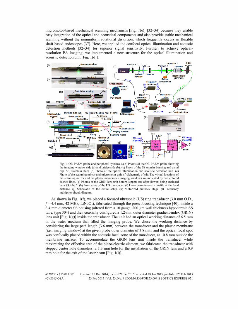
Fig. 1. OR-PAEM probe and peripheral systems. (a,b) Photos of the OR-PAEM probe showing the imaging window side (a) and bridge side (b). (c) Photo of the SS tubular housing and distal cap. SS, stainless steel. (d) Photo of the optical illumination and acoustic detection unit. (e) Photo of the scanning mirror and micromotor unit. (f) Schematic of (d). The virtual locations of the scanning mirror and the plastic membrane (imaging window) are indicated by two colored dashed lines. (g) Photos of the GRIN lens unit before (upper) and after (lower) being enclosed by a SS tube 2. (h) Front view of the US transducer. (i) Laser beam intensity profile at the focal distance. (j) Schematic of the entire setup. (k) Motorized pullback stage. (l) Frequency multiplier circuit diagram.

As shown in Fig. 1(f), we placed a focused ultrasonic (US) ring transducer (3.0 mm O.D., f = 4.4 mm, 42 MHz, LiNbO3), fabricated through the press-focusing technique [40], inside a 3.4 mm diameter SS housing (altered from a 10 gauge, 200 µm wall thickness hypodermic SS tube, type 304) and then coaxially configured a 1.2-mm outer diameter gradient-index (GRIN) lens unit [Fig. 1(g)] inside the transducer. The unit had an optical working distance of 6.5 mm in the water medium that filled the imaging probe. We chose the working distance by considering the large path length (3.6 mm) between the transducer and the plastic membrane (i.e., imaging window) at the given probe outer diameter of 3.8 mm, and the optical focal spot was confocally placed within the acoustic focal zone of the transducer, at ~0.8 mm outside the membrane surface. To accommodate the GRIN lens unit inside the transducer while maximizing the effective area of the piezo-electric element, we fabricated the transducer with stepped center hole diameters: a 1.3 mm hole for the installation of the GRIN lens and a 0.9 mm hole for the exit of the laser beam [Fig. 1(i)].


As shown in Fig. 1(g), the GRIN lens unit was enclosed in an SS tube (1.2 mm O.D., 1.0 mm I.D.; altered from a 17 gauge, 254 µm wall thickness hypodermic SS tube, type 304) and completely sealed with epoxy at both ends to avoid water permeation. To achieve the maximal optical numerical aperture (NA) at the given working distance, we utilized a custom ordered GRIN lens (0.20 pitch, GRINTECH GmbH) with a 0.5 mm outer diameter and 2.4 mm length. Inside the SS tube, the GRIN lens was coupled with a single-mode optical fiber (SM600, Thorlabs), which guided the laser beam from a light source. The distance between the optical fiber’s tip and the beam entrance surface of the GRIN lens was set at 0.8 mm. This distance and the pitch of the GRIN lens were determined from a ZEMAX simulation. Importantly, we chose the above shown [Fig. 1(g)], glass ferrule-based affixing method to assemble the GRIN lens and optical fiber, instead of directly attaching a GRIN lens [13] with a different pitch, because it is not desirable to have any glued interface along the beam path or an intermediately formed focused zone of the laser beam inside the GRIN lens, owing to the high laser energy flux with a high-pulse repetition rate. After completing the GRIN lens unit [Fig. 1(g)], we analyzed the output beam profile using a beam profiler (SP620U, OPHIR Beam Gauge) and measured the FWHM-based beam diameter to be ~9.2 µm [Fig. 1(i)] – this value yields a beam waist size (ѡ0) of 7.8 µm and an optical NA of ~0.022 under the assumption of a Gaussian beam.

In realizing the OR-PAEM probe, one of the most crucial processes was to provide acoustic matching for the inner cavity of the imaging probe to efficiently transmit generated PA waves to the US transducer. Unlike the flexible shaft-based proximal actuation mechanism [37], which delivers mechanical torque from an external source, the scanning mirror and built-in micromotor-based mechanical scanning mechanism advantageously solves the acoustic matching requirement because all the moving parts of the imaging probe are housed in an isolated space of the distal section [Fig. 1(a)]. To provide acoustic matching inside the probe, we implemented the probe so that liquid could be injected – in this study, we utilized deionized water as the matching medium because it exhibits both high optical transparency and low acoustic attenuation for high-frequency acoustic waves. As shown in Figs. 1(d) and 1(f), we installed a SS hypodermic tube (28 gauge, 76 µm wall thickness, ~2 cm length, type 304) at the base of the GRIN lens and transducer unit for water injection, and also installed another SS hypodermic tube (30 gauge, ~1 cm length, 102 µm wall thickness, type 304) at a side of the mechanical unit for water drainage [Fig. 1(e)], which will be explained later. The water injection SS tube is further extended by a ~50 cm long plastic tube (762 µm O.D., 254 µm I.D., Tygon) along the flexible body section. Thus, the flexible body section of the probe is comprised of the optical fiber (~2 m length), the water injection plastic tube (~50 cm length), the signal wire (38 AWG, 50 Ω, ~1 m length, New England Wire Technologies) of the transducer, the four electric wires of the micromotor (~2 m length), and an additional narrow diameter SS tubular stiffener (30 gauge, ~50 cm length) to reinforce the flexible body section. All of these components are then fully sheathed with a ~30 cm long polyethylene terephthalate (PET, Advanced Polymers) plastic tube (see section 1 in Fig. 1(b)), with the procedure described in section 2.4.

The overall structure of the probe and the water injection unit was similar to that of previous PAE probes [32–34]. However, we improved the overall mechanical performance and the water injection function by modifying the related designs slightly. To fabricate the endomicroscope, we utilized standard size medical grade hypodermic SS tubes purchased from either MicroGroup or McMaster-Carr, and utilized several different medical grade adhesives with different viscosities and curing times, such as M-31CL (Loctite), Loctite 4014 (Loctite), and DP-125 (3M). To form the imaging window of the endomicroscope [Fig. 1(a)], we utilized a PET heat shrink tube (140150CST, 3.56 mm average expanded diameter, 38 µm wall thickness, Advanced Polymers) because it exhibits good optical and acoustic transparency and also is relatively easy to glue compared to other plastic materials. We used an ordinary UV-curing optical adhesive (NOA68, Norland Products, purchased from


Thorlabs) to seal the gap between the tubular imaging window and the SS housing. To form the metal housing of the endomicroscope [Fig. 1(c)], we utilized 9 gauge (178 µm wall thickness) and 10 gauge (254 µm wall thickness for the imaging window section and 203 µm wall thickness for the mechanical unit adapter installed at the tip of the housing) SS hypodermic tubes (type 304). More detailed information on the mechanical parts of the imaging probe is available elsewhere [33].

2.2 Peripheral systems

For PA imaging, we developed peripheral systems as shown in Fig. 1(j). We utilized a Q-switched diode-pumped Nd:YAG laser (SPOT 10-200-532, Elforlight) that provided a 532-nm wavelength with a pulse duration of ~1 ns. A portion of the laser beam was selected by an aperture (1.3 mm diameter) and a variable neutral density (ND) filter (NDC-50C-4, Thorlabs), then focused into a 50-µm diameter pinhole (#59-261, Edmund) by a convex lens (f = 10 cm) for spatial filtering. After the filtration, the beam was collimated by a convex lens (f = 30 cm), further shaped by an aperture (4.0 mm diameter), and focused into the input of the endomicroscope’s optical fiber by a 10× objective lens. Finally, to generate PA waves, the beam was delivered to the target tissue via the optical fiber, the GRIN lens, and the scanning mirror. Once PA waves were generated, some of them were reflected by the same mirror, sent to the transducer, converted into electrical signals, amplified by an amplifier (5073PR, Panametrics), and digitally recorded by a data acquisition (DAQ) card (200 MHz, NI PCI-5124, National Instruments). Throughout the experiments, the output energy of laser beam at the GRIN lens aperture was regulated to be ~500 nJ/pulse by adjusting the ND filter, based on the readout power value provided by the optical power meter (PM20A, Thorlabs) shown in Fig. 1(j). Since we knew that the energy delivery efficiency from the output of aperture 2 to the output of the GRIN lens unit was about 35%, and 30% to the optical power meter, we could estimate the output power at the GRIN lens unit. Under the assumption of a Gaussian beam, this energy yields a surface fluence of ~44 mJ/cm2, which is about two times greater than the ANSI safety limit (20 mJ/cm2) for allowable skin laser fluence [41] but below the damage threshold (200 mJ/cm2) [41].

For this endomicroscope, we utilized the same type of micromotor (SBL015-06XXPG254; Namiki Precision) as employed in our previous endoscopic probes [32–34] because of its superior torque and scanning speed. Also, as before [32–34], we used the scanning mirror’s angular position-encoded TTL signals (254 pulses at ~1 kHz per one full mirror rotation) to synchronously trigger peripheral systems, such as the laser and the DAQ card [Fig. 1(j)]. However, because the optical beam diameter determines the transverse resolution of OR-PAEM, it is important to provide a sufficient A-line sampling density for each B-scan such that consecutive optical beams overlap. Therefore, we implemented another circuit that multiplies the original TTL frequency by eight times [Fig. 1(l)], i.e., 2032 pulses at ~8 kHz for one full mirror rotation. In other words, we performed OR-PAEM imaging with an A-line acquisition rate of ~8 kHz and a B-scan rate of 4 Hz, which is also the rotational speed of the scanning mirror; each B-scan consists of 2032 A-lines.

As discussed earlier [34], another advantage of the scanning mirror and built-in micromotor-based mechanical scanning mechanism is that it enables static mounting of the optical fiber and signal wires. Thus, it is possible to perform a pullback C-scan over a large interval without the aid of a sophisticated pullback system. In this study, we utilized a previously-constructed motorized pullback system [34] which includes a step motor and a linear motion guide actuator (KR2001A+200L0-0000, THK) with a stroke of ~14 cm [Fig. 1(k)]. To synchronously control the pullback pitch in accordance with the rotation of the scanning mirror, we utilized the TTL signals provided by the delay generator, in which a counter circuit was also installed to adjust the pullback pitch, as shown in Fig. 1(j).


2.3 Quantifying the US transducer’s acoustic performance and combining it with the GRIN lens unit

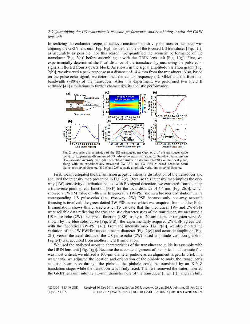
In realizing the endomicroscope, to achieve maximum sensitivity the most critical step was aligning the GRIN lens unit [Fig. 1(g)] inside the hole of the focused US transducer [Fig. 1(f)] as accurately as possible. For this reason, we quantified the acoustic performance of the transducer [Fig. 2(a)] before assembling it with the GRIN lens unit [Fig. 1(g)]. First, we experimentally determined the focal distance of the transducer by measuring the pulse-echo signals reflected from a quartz block. As shown in the signal amplitude variation graph [Fig. 2(b)], we observed a peak response at a distance of ~4.4 mm from the transducer. Also, based on the pulse-echo signal, we determined the center frequency (42 MHz) and the fractional bandwidth (~80%) of the transducer. After this experiment, we performed two Field II software [42] simulations to further characterize its acoustic performance.

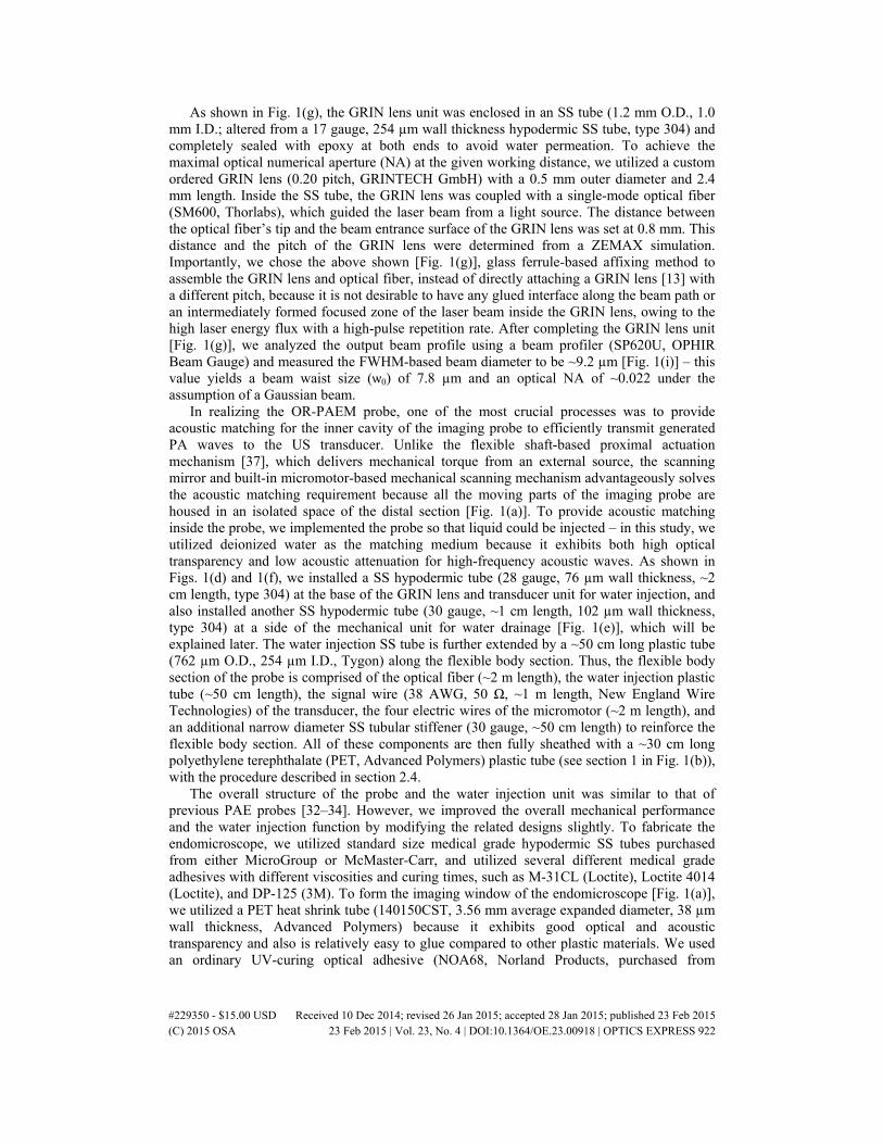
Fig. 2. Acoustic characteristics of the US transducer. (a) Geometry of the transducer (side view). (b) Experimentally measured US pulse-echo signal variation. (c) Simulated transmission (1W) acoustic intensity map. (d) Theoretical transverse 1W- and 2W-PSFs on the focal place, along with an experimentally measured 2W-LSF. (e) 1W FWHM-based acoustic beam diameter vs. axial distance. (f) 1W and 2W acoustic amplitude variations vs. axial distance.

First, we investigated the transmission acoustic intensity distribution of the transducer and acquired the intensity map presented in Fig. 2(c). Because this intensity map implies the one-way (1W) sensitivity distribution related with PA signal detection, we extracted from the map a transverse point spread function (PSF) for the focal distance of 4.4 mm [Fig. 2(d)], which showed a FWHM value of ~86 µm. In general, a 1W-PSF shows a broader distribution than a corresponding US pulse-echo (i.e., two-way: 2W) PSF because only one-way acoustic focusing is involved; the green dotted 2W-PSF curve, which was acquired from another Field II simulation, shows this characteristic. To validate that the theoretical 1W- and 2W-PSFs were reliable data reflecting the true acoustic characteristics of the transducer, we measured a US pulse-echo (2W) line spread function (LSF), using a ~20 µm diameter tungsten wire. As shown by the blue solid curve [Fig. 2(d)], the experimentally acquired 2W-LSF agrees well with the theoretical 2W-PSF [43]. From the intensity map [Fig. 2(c)], we also plotted the variation of the 1W FWHM acoustic beam diameter [Fig. 2(e)] and acoustic amplitude [Fig. 2(f)] versus the axial distance; the US pulse-echo (2W) based amplitude variation graph in Fig. 2(f) was acquired from another Field II simulation.

We used the analyzed acoustic characteristics of the transducer to guide its assembly with the GRIN lens unit [Fig. 1(g)]. Because the accurate alignment of the optical and acoustic foci was most critical, we utilized a 100-µm diameter pinhole as an alignment target. In brief, in a water tank, we adjusted the location and orientation of the pinhole to make the transducer’s acoustic beam pass through the pinhole; the pinhole could be translated by an X-Y-Z translation stage, while the transducer was firmly fixed. Then we removed the water, inserted the GRIN lens unit into the 1.3-mm diameter hole of the transducer [Fig. 1(f)], and carefully


aligned it so that the transmitted laser beam also passed through the pinhole. We performed the final alignment solely by manually positioning the GRIN lens unit while 5-minutes epoxy spread around the base of the GRIN lens and transducer unit [Fig. 1(f)] started to cure. A post-assembly measurement showed that the mismatch between the acoustic focus and optical focus was less than 32 µm in the transverse plane. As shown in Fig. 2(e), the transducer showed a somewhat constant maximal focal zone (i.e., a plateau) over a large range, from 3.8 mm to 5.3 mm; just outside these two positions, the acoustic intensity of the side lobes started to become greater than the half values of their maxima (i.e., –6 dB), widening the FWHM beam diameter steeply. The large depth of acoustic focus facilitated the longitudinal alignment of the laser beam and acoustic beam.

2.4 Pre-imaging procedure: providing acoustic matching and sheathing

As mentioned in section 2.1, we utilize deionized water as the matching medium of the inner cavity. However, it gradually corrodes the metallic components and degrades the glued points. Thus, the three key units shown in Figs. 1(c)–1(e) were designed to facilitate water injection before each experiment and drainage after each experiment. Originally we intended to inject water after combining the SS tubular housing of the probe [Fig. 1(c)] with the GRIN lens and transducer unit [Fig. 1(d)] as well as the mechanical unit [Fig. 1(e)], but before closing the cap shown in Fig. 1(c). However, we found that, although it is certainly possible, it takes a very long time and it is very difficult to inject water without bubbles (we performed an experiment including some bubbles; however, the image quality was poor). Thus, we switched the water injection procedure to a new method in which we assemble the three key units submerged in a clean water tank. Figure 3 shows the detailed procedure.

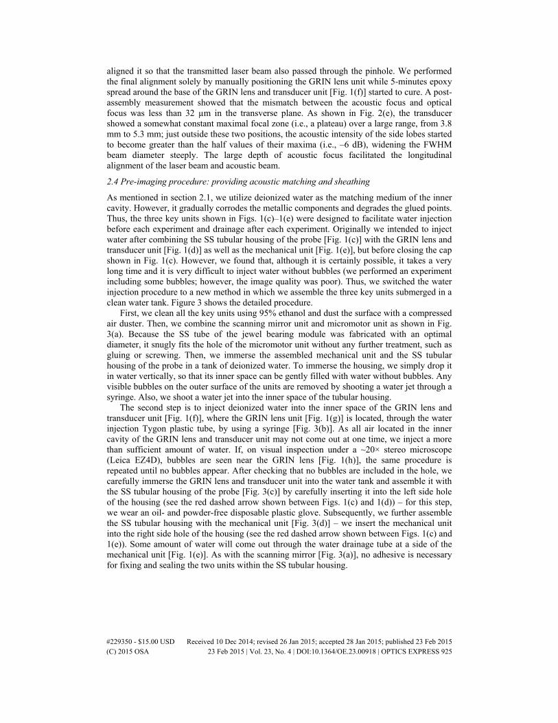
First, we clean all the key units using 95% ethanol and dust the surface with a compressed air duster. Then, we combine the scanning mirror unit and micromotor unit as shown in Fig. 3(a). Because the SS tube of the jewel bearing module was fabricated with an optimal diameter, it snugly fits the hole of the micromotor unit without any further treatment, such as gluing or screwing. Then, we immerse the assembled mechanical unit and the SS tubular housing of the probe in a tank of deionized water. To immerse the housing, we simply drop it in water vertically, so that its inner space can be gently filled with water without bubbles. Any visible bubbles on the outer surface of the units are removed by shooting a water jet through a syringe. Also, we shoot a water jet into the inner space of the tubular housing.

The second step is to inject deionized water into the inner space of the GRIN lens and transducer unit [Fig. 1(f)], where the GRIN lens unit [Fig. 1(g)] is located, through the water injection Tygon plastic tube, by using a syringe [Fig. 3(b)]. As all air located in the inner cavity of the GRIN lens and transducer unit may not come out at one time, we inject a more than sufficient amount of water. If, on visual inspection under a ~20× stereo microscope (Leica EZ4D), bubbles are seen near the GRIN lens [Fig. 1(h)], the same procedure is repeated until no bubbles appear. After checking that no bubbles are included in the hole, we carefully immerse the GRIN lens and transducer unit into the water tank and assemble it with the SS tubular housing of the probe [Fig. 3(c)] by carefully inserting it into the left side hole of the housing (see the red dashed arrow shown between Figs. 1(c) and 1(d)) – for this step, we wear an oil- and powder-free disposable plastic glove. Subsequently, we further assemble the SS tubular housing with the mechanical unit [Fig. 3(d)] – we insert the mechanical unit into the right side hole of the housing (see the red dashed arrow shown between Figs. 1(c) and 1(e)). Some amount of water will come out through the water drainage tube at a side of the mechanical unit [Fig. 1(e)]. As with the scanning mirror [Fig. 3(a)], no adhesive is necessary for fixing and sealing the two units within the SS tubular housing.


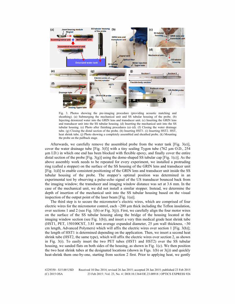
Fig. 3. Photos showing the pre-imaging procedure (providing acoustic matching and sheathing). (a) Submerging the mechanical unit and SS tubular housing of the probe. (b) Injecting deionized water into the GRIN lens and transducer unit. (c) Inserting the GRIN lens and transducer unit into the SS tubular housing. (d) Inserting the mechanical unit into the SS tubular housing. (e) Photo after finishing procedures (a)–(d). (f) Closing the water drainage tube. (g) Closing the distal section of the probe. (h) Inserting HST1. (i) Inserting HST2. HST, heat shrink tube. (j) Photo showing a completely assembled and sheathed probe. (k) Mounting the probe on the pullback stage.

Afterwards, we carefully remove the assembled probe from the water tank [Fig. 3(e)], cover the water drainage tube [Fig. 3(f)] with a tiny sealing Tygon tube (762 µm O.D., 254 µm I.D.) in which one end has been blocked with flexible epoxy, and finally cover the entire distal section of the probe [Fig. 3(g)] using the dome-shaped SS tubular cap [Fig. 1(c)]. As the above assembly work needs to be repeated for every experiment, we installed a protruding ring (called a stopper) on the surface of the SS housing of the GRIN lens and transducer unit [Fig. 1(d)] to enable consistent positioning of the GRIN lens and transducer unit inside the SS tubular housing of the probe. The stopper’s optimal position was determined in an experimental test by observing a pulse-echo signal of the US transducer bounced back from the imaging window; the transducer and imaging window distance was set at 3.6 mm. In the case of the mechanical unit, we did not install a similar stopper. Instead, we determine the depth of insertion of the mechanical unit into the SS tubular housing based on the visual inspection of the output point of the laser beam [Fig. 1(a)].

The third step is to secure the micromotor’s electric wires, which are comprised of four electric wires for the micromotor control, each ~200 µm thick including the Teflon insulation, over sections 1 and 2 (see Fig. 1(b) or Fig. 3(j)). First, we carefully align the four motor wires on the surface of the SS tubular housing along the bridge of the housing located at the imaging window section (see Fig. 1(b)), and insert a very thin medical grade heat shrink tube (HST1, PET, 150100CST, 3.81 mm average expanded diameter, 25 µm wall thickness, ~30 cm length, Advanced Polymers) which will affix the electric wires over section 1 [Fig. 3(h)]; the length of HST1 is determined depending on the application. Then, we insert a second heat shrink tube (HST2, the same type), which will affix the electric wires over section 2, as shown in Fig. 3(i). To easily insert the two PET tubes (HST1 and HST2) over the SS tubular housing, we sanded flats on both sides of the housing, as shown in Fig. 1(c). We then position the two heat shrink tubes at the designated locations (shown in Figs. 1(b) or 3(j)) and quickly heat-shrink them one-by-one, starting from section 2 first. Prior to applying heat, we gently


pull the electric wires straight. In shrinking the tubes, it is important to avoid deforming the imaging window, which is made of the same material, PET. Thus, prior to applying heat, we wrap the imaging window section using a small piece of wet cloth (~1 cm × 5 cm), apply heat, and immediately cool the heated area to avoid possible thermal damage to the components inside the probe. Figure 3(j) shows a photo of the probe sheathed with the two heat shrink tubes.

By assembling and sheathing the probe as explained, all the optical, acoustical, and mechanical components are completely isolated in the streamlined SS tubular housing and the medical grade PET tubes, which yields a total outer diameter of ~3.8 mm. We then clean the surface of the probe using ethanol and tape the probe onto the flat surface of the pullback stage, as shown in Fig. 3(k). To complete the entire assembly procedure, we usually spend about 40–60 minutes. Although repeating the presented procedure for each imaging session is undesirable, this underwater assembly and sheathing method yielded much better imaging results than the post-assembly water injection method mentioned above. After we finish an imaging experiment, we disassemble the three key units and put them into 95% ethanol to replace corrosive water with ethanol, which quickly evaporates. In our earlier work [34], we utilized Teflon tube for sheathing the flexible body section (see Fig. 3(j)), but the same PET for other sections. However, we switched to PET for all the sheathing of the probe because it can be easily removed (i.e., single-use) using a standard surgical blade (#11).

3. Quantification of system resolution and sensitivity

First, we imaged an optical phantom made of 3 µm diameter polystyrene black dyed microspheres (#605633, Polysciences) and gelatin (#G2500, Sigma–Aldrich) [Fig. 4(a)]. In the phantom, the concentrations of the microspheres and gelatin were 0.009% and 10% (w/v), respectively, when they were dissolved in water. Figure 4(b) is a light microscopic image (×100) of a drop of the mixture before it hardened. After spreading ultrasound gel on the surface of the phantom for acoustic matching [Fig. 4(a)], we positioned the endomicroscope, performed a pullback C-scan with a pitch of 1 µm, and recorded 2000 B-scan images during the helical motion of the scanning mirror. For this experiment, however, we did not use the TTL signals provided by the frequency multiplier [Fig. 1(j)] because the desired transverse step size of the scanning mirror was smaller than the theoretical transverse resolution value of ~9.2 µm. Thus, we utilized a 16-kHz TTL signal provided by a function generator for triggering the DAQ and laser system and also reduced the B-scan speed to 2 Hz, which resulted in an angular step size for the scanning mirror ¼ of the theoretical transverse resolution value.

In Fig. 4(c), we present a B-scan image acquired from the phantom (only a 90° angular region is displayed). As the microspheres were embedded randomly in the phantom, they generated sharp spike signals with different intensities according to depth. So, by plotting all A-line signals that included such spike signals over the entire data set [Fig. 4(d)], we were able to validate the targeted location of the optical focus and also estimate the sensitivity of the endomicroscope. From the graph, one can see that the signal sensitivities show a clear depth dependency following the diameter variation of the laser beam, and that the strongest signal appeared at the focal distance of the optical illumination (i.e., ~0.8 mm from the probe surface, as we intended), as shown by the artificially marked dashed curve. To estimate the radial resolution and signal-to-noise ratio (SNR), we selected a set of PA signals generated by a microsphere located at the focal distance from Fig. 4(d) and plotted them in Fig. 4(e). As shown in Fig. 4(f), from this specific microsphere, the radial resolution was estimated to be ~50 µm, and the SNR appeared to be approximately 29 dB; PA signals from other microspheres also yielded the same radial resolution value.


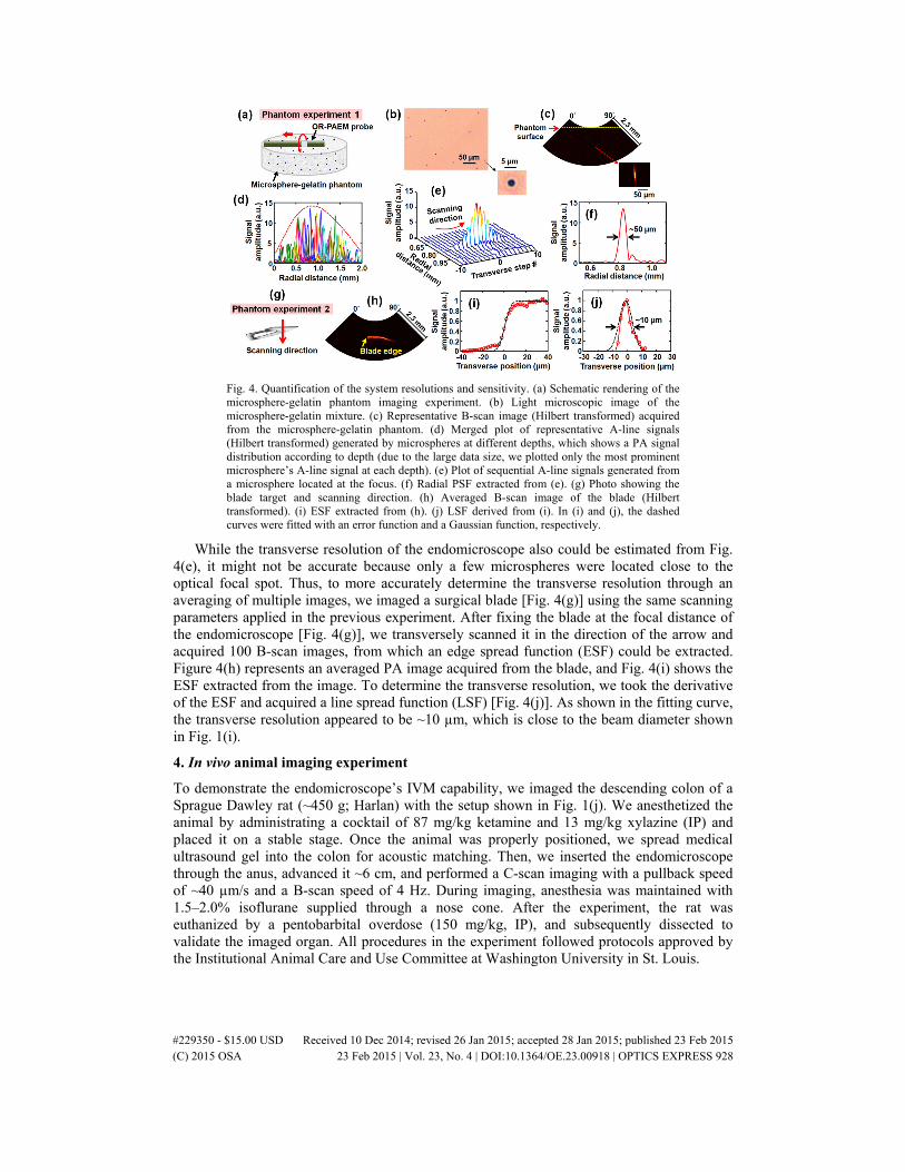
Fig. 4. Quantification of the system resolutions and sensitivity. (a) Schematic rendering of the microsphere-gelatin phantom imaging experiment. (b) Light microscopic image of the microsphere-gelatin mixture. (c) Representative B-scan image (Hilbert transformed) acquired from the microsphere-gelatin phantom. (d) Merged plot of representative A-line signals (Hilbert transformed) generated by microspheres at different depths, which shows a PA signal distribution according to depth (due to the large data size, we plotted only the most prominent microsphere’s A-line signal at each depth). (e) Plot of sequential A-line signals generated from a microsphere located at the focus. (f) Radial PSF extracted from (e). (g) Photo showing the blade target and scanning direction. (h) Averaged B-scan image of the blade (Hilbert transformed). (i) ESF extracted from (h). (j) LSF derived from (i). In (i) and (j), the dashed curves were fitted with an error function and a Gaussian function, respectively.

While the transverse resolution of the endomicroscope also could be estimated from Fig. 4(e), it might not be accurate because only a few microspheres were located close to the optical focal spot. Thus, to more accurately determine the transverse resolution through an averaging of multiple images, we imaged a surgical blade [Fig. 4(g)] using the same scanning parameters applied in the previous experiment. After fixing the blade at the focal distance of the endomicroscope [Fig. 4(g)], we transversely scanned it in the direction of the arrow and acquired 100 B-scan images, from which an edge spread function (ESF) could be extracted. Figure 4(h) represents an averaged PA image acquired from the blade, and Fig. 4(i) shows the ESF extracted from the image. To determine the transverse resolution, we took the derivative of the ESF and acquired a line spread function (LSF) [Fig. 4(j)]. As shown in the fitting curve, the transverse resolution appeared to be ~10 µm, which is close to the beam diameter shown in Fig. 1(i).

4. In vivo animal imaging experiment

To demonstrate the endomicroscope’s IVM capability, we imaged the descending colon of a Sprague Dawley rat (~450 g; Harlan) with the setup shown in Fig. 1(j). We anesthetized the animal by administrating a cocktail of 87 mg/kg ketamine and 13 mg/kg xylazine (IP) and placed it on a stable stage. Once the animal was properly positioned, we spread medical ultrasound gel into the colon for acoustic matching. Then, we inserted the endomicroscope through the anus, advanced it ~6 cm, and performed a C-scan imaging with a pullback speed of ~40 µm/s and a B-scan speed of 4 Hz. During imaging, anesthesia was maintained with 1.5–2.0% isoflurane supplied through a nose cone. After the experiment, the rat was euthanized by a pentobarbital overdose (150 mg/kg, IP), and subsequently dissected to validate the imaged organ. All procedures in the experiment followed protocols approved by the Institutional Animal Care and Use Committee at Washington University in St. Louis.


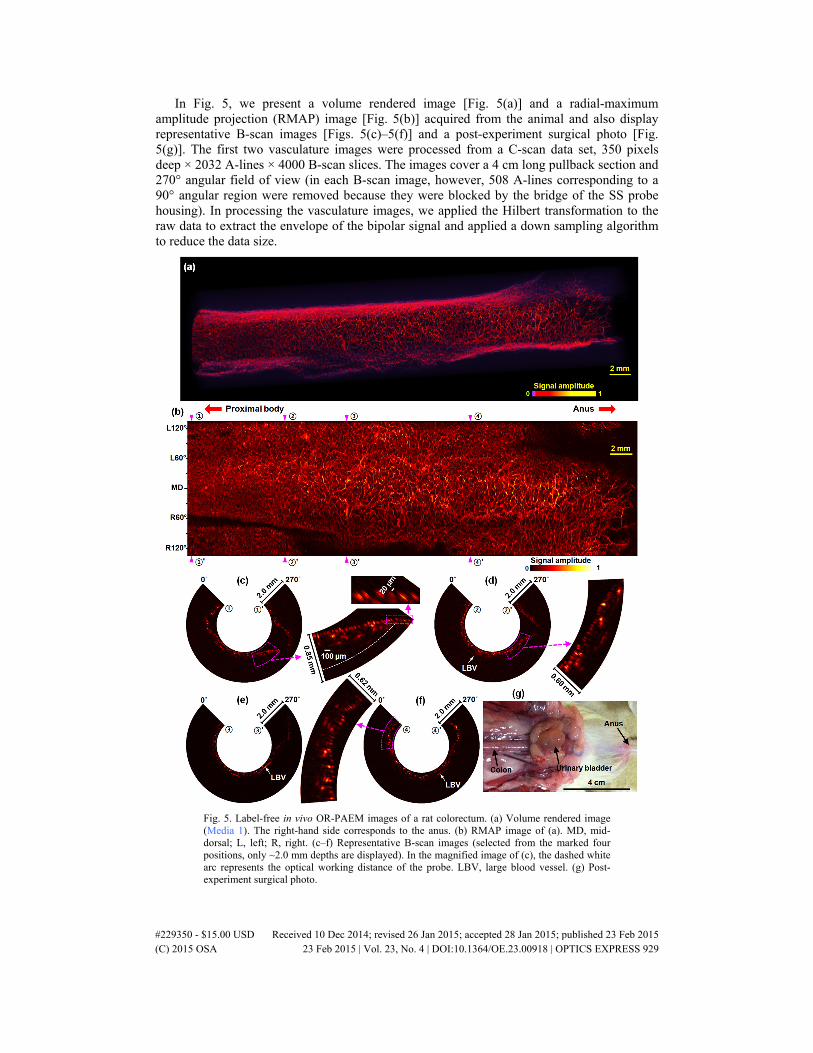
In Fig. 5, we present a volume rendered image [Fig. 5(a)] and a radial-maximum amplitude projection (RMAP) image [Fig. 5(b)] acquired from the animal and also display representative B-scan images [Figs. 5(c)–5(f)] and a post-experiment surgical photo [Fig. 5(g)]. The first two vasculature images were processed from a C-scan data set, 350 pixels deep × 2032 A-lines × 4000 B-scan slices. The images cover a 4 cm long pullback section and 270° angular field of view (in each B-scan image, however, 508 A-lines corresponding to a 90° angular region were removed because they were blocked by the bridge of the SS probe housing). In processing the vasculature images, we applied the Hilbert transformation to the raw data to extract the envelope of the bipolar signal and applied a down sampling algorithm to reduce the data size.

Fig. 5. Label-free in vivo OR-PAEM images of a rat colorectum. (a) Volume rendered image (Media 1). The right-hand side corresponds to the anus. (b) RMAP image of (a). MD, mid-dorsal; L, left; R, right. (c–f) Representative B-scan images (selected from the marked four positions, only ~2.0 mm depths are displayed). In the magnified image of (c), the dashed white arc represents the optical working distance of the probe. LBV, large blood vessel. (g) Post-experiment surgical photo.


http://www.opticsinfobase.org/boe/viewmedia.cfm?uri=boe-6-3-918-1

As shown in the RMAP image [Fig. 5(b)], the endomicroscope provided a much clearer view of the colorectal vasculature than the previous acoustic-resolution PA endoscopic images [32–37]; based on the estimation of apparent blood vessel diameters, approximately a 10-fold improvement in spatial resolution was achieved. Also, the capillaries distributed in the inner wall of the colorectum were clearly differentiated [Fig. 5(c)] with the full resolving power presented in Fig. 4. Due to motion artifacts and the large variation in colorectal wall distances [Fig. 5(c)], however, the apparent resolution in the RMAP image was slightly degraded during the composition of individual B-scan slices. Nevertheless, the prototype probe imaged the colorectal vasculature with an apparent resolution of less than 30 µm. To more clearly display the densely distributed lattice-like vascular networks [Fig. 5(b)], we present the volume-rendered image [Fig. 5(a)] as a multimedia (Media 1).

With the current sensitivity of the transducer and a laser power of 500 nJ, we were able to detect PA signals from a ~500 µm depth, which was enough to encompass the entire thickness of the colorectal wall (~400 µm) and visualize some of neighboring large blood vessels (LBVs) [Figs. 5(d)–5(f)] which are assumed to be the blood vessels connecting the colorectum and mesenteric tissue. The 500-nJ pulse energy was somewhat higher than the values typically utilized in OR-PAM systems. However, the laser beam diameter at the focal distance was also correspondingly larger; the low optical NA of 0.022 was also advantageous in maintaining the optical resolving power over a large depth range.

5. Summary and discussion

In this study, we showed the feasibility of PAT-based IVM for the first time by implementing a fully-encapsulated OR-PAEM probe and imaging the microvasculature of a rat colorectum. With an optical NA of 0.022, we achieved a transverse resolution as fine as 10 µm, the finest among reported optical-resolution endoscopic PA images [38, 39], and an SNR of 29 dB from a 3-µm diameter microsphere illuminated by a 500-nJ pulse energy in a beam 9.2 µm in diameter. As demonstrated in the in vivo experiment, the major benefit of OR-PAEM over existing IVM techniques [1–13] is that it enables high-resolution angiographic imaging without using a contrast agent. Although other groups have achieved comparable resolutions [38, 39], their image demonstrations were limited to only phantom experiments because their probes are not fully encapsulated. We achieved the first in vivo OR-PAEM imaging by combining the confocal focused-optical illumination and acoustic detection scheme with our established probe encapsulation and acoustic matching strategy [32–34], which is one of the most important technical elements.

Although the acoustic matching and probe sheathing method presented in section 2.4 is not simple and requires a long preparation time (40–60 minutes), we believe it could be a valuable technical basis for developing more advanced PA endoscopic systems. For example, the water injection strategy and associated system elements could be applied to using such an OR-PAEM probe with a medical balloon, which is frequently utilized for mitigating motion artifacts [5] in various clinical environments. One possible option for slightly reducing the long assembly time is to build the GRIN lens and transducer unit [Fig. 1(d)] without the gap within them [Fig. 1(f)], by which one can skip the long (~15 minutes) water injection time (i.e., the second step in section 2.4). However, as we discussed in our recent report [34], the entire acoustic matching and probe sheathing process could be completely avoided if the corrosive water-based matching medium could be replaced with an oil-based medium which could be retained in the probe perpetually. So far, we have tried a silicone oil-based medium. However, we found that, although silicone oil was superior in terms of optical transparency, it turned out to be inapplicable to the current probe configuration because the large travel distance (3.6 mm) from the membrane to the transducer caused large acoustic attenuation of high-frequency acoustic waves. Thus, high optical transparency and low acoustic attenuation must be considered as key requirements for PA endoscopy.


http://www.opticsinfobase.org/boe/viewmedia.cfm?uri=boe-6-3-918-1

To make the developed technique more broadly applicable, several additional technical advances should be achieved. The first is to embody a multi-wavelength OR-PAEM system. In this study, we demonstrated the vasculature imaging capability of the implemented endomicroscope by using a 532 nm laser wavelength. We chose the wavelength due to the availability of laser sources with a high pulse-repetition rate (~8 kHz). For in vivo vasculature imaging, however, other wavelengths, such as 542 nm and 576 nm, are known to be generally better in terms of the SNR of detected PA signals at a given pulse energy because oxy-hemoglobin shows high optical absorption at those wavelengths [44]. Also, one can choose other wavelengths for visualizing various functional information, such as the oxygen saturation of hemoglobin, or molecular information, such as the distribution of various contrast agents or molecular probes [15–18]. In general, PAT systems are developed for imaging objects over large depths. Thus, one can choose an optimal wavelength to increase the imaging depth. However, OR-PAM or OR-PAEM are not noted for their depth capability: their typical imaging depth is ~1 mm, and they are more affected by optical scattering. Thus, one can choose the wavelength according to the optical absorption peak of the contrast agent of interest, either endogenous or exogenous.

The second important task is to increase the sensitivity of the imaging probe. In this study, we achieved an adequate SNR with an optical energy of ~500 nJ/pulse, which yields a surface fluence of ~44 mJ/cm2, about two times greater than the ANSI safety limit (20 mJ/cm2) for allowable skin laser fluence [41]. Although this value is lower than the damage threshold of general tissue (200 mJ/cm2) [41], it would not be desirable to use for internal organ imaging, especially for clinical applications (currently there is no explicit and specific reference on the pulsed laser beam dose to use with PAT. However, we observed no damage with the typical fluence applied to human skin). We believe that the laser dose can be substantially reduced by employing more sensitive ultrasound detectors, such as lead magnesium niobate-lead titanate (PMN-PT)-based US transducer [45] or optical ultrasound detectors [39, 46, 47].

To use OR-PAEM as an even higher resolution IVM imaging tool, the third task is to increase the spatial resolution. Although we showed the feasibility of OR-PAEM imaging, the resolution benefit was limited to only the transverse direction, and the radial (depth) resolution was still limited by the acoustic parameters of the employed US transducer. Thus, in the in vivo rat colorectum imaging [Fig. 5], we were not able to clearly differentiate blood vessels in different layers of the colorectum. Consequently, increasing the radial resolution could be an interesting research subject. It is a well-known fact that achieving high-radial resolution with PAT is relatively difficult compared to other optical microscopy techniques, such as two-photon microscopy. However, a recent study reported by Wang et al. demonstrated that it could be feasible in OR-PAM [48]. In an in vitro condition, they achieved a 2.3 µm radial resolution. Also, one can increase the transverse resolution by increasing the optical NA, at the expense of the depth of focus, and optimize the working distance depending on target applications. To acquire high resolution PA images, however, the imaging speed should be increased together with resolution, because motion artifacts deteriorate the apparent resolution.

6. Conclusion

In this study, we implemented the first OR-PAEM system with a full IVM imaging capability and achieved a transverse resolution as low as 10 µm, the finest among reported optical-resolution endoscopic PA images, and an SNR of 29 dB for a 3-µm diameter microsphere illuminated by a 500-nJ pulse energy in a beam of 9.2 µm in diameter. Also, by using a 532-nm laser wavelength, we acquired the first in vivo OR-PAEM image from a rat colorectum and produced a three-dimensional vasculature image with an apparent resolution of less than 30 µm. As the system can be utilized in small animals and also can potentially accommodate many other multi-functional molecular probes, it could be a useful tool in many biological experiments, such as tumor and metabolic disease studies. Moreover, the OR-PAEM’s unique


label-free imaging capability would enhance IVM’s role in such clinical circumstances where the uses of contrast agents are undesired.

Acknowledgments

We thank Prof. James Ballard for his attentive reading of the manuscript. This work was sponsored in part by National Institutes of Health grants R01 CA157277, DP1 EB016986 (NIH Director’s Pioneer Award), P41-EB002182, and R01 CA186567 (NIH Director’s Transformative Research Award). L.W. has a financial interest in Microphotoacoustics, Inc. and Endra, Inc., which, however, did not support this work. K.M. has a financial interest in Microphotoacoustics, Inc.


Documents

Optical-resolution photoacoustic endomicroscopy in vivocoilab.caltech.edu/epub/2015/YangJM_2015_Biomedical Optics Express... · Optical-resolution photoacoustic endomicroscopy in