Optimal Experimental Design for Another's Analysis

Optimal Experimental Design for Another's AnalysisAuthor(s): Ruth Etzioni and Joseph B. KadaneSource: Journal of the American Statistical Association, Vol. 88, No. 424 (Dec., 1993), pp. 1404-1411Published by: American Statistical AssociationStable URL: http://www.jstor.org/stable/2291284 .

Accessed: 14/06/2014 09:51

Your use of the JSTOR archive indicates your acceptance of the Terms & Conditions of Use, available at .http://www.jstor.org/page/info/about/policies/terms.jsp

.JSTOR is a not-for-profit service that helps scholars, researchers, and students discover, use, and build upon a wide range ofcontent in a trusted digital archive. We use information technology and tools to increase productivity and facilitate new formsof scholarship. For more information about JSTOR, please contact [email protected].

.

American Statistical Association is collaborating with JSTOR to digitize, preserve and extend access to Journalof the American Statistical Association.

http://www.jstor.org

This content downloaded from 195.34.79.49 on Sat, 14 Jun 2014 09:51:32 AMAll use subject to JSTOR Terms and Conditions

http://www.jstor.org/action/showPublisher?publisherCode=astata

http://www.jstor.org/stable/2291284?origin=JSTOR-pdf

http://www.jstor.org/page/info/about/policies/terms.jsp


Optimal Experimental Design for Another's Analysis Ruth ETZIONI and Joseph B. KADANE *

We consider the optimal design of experiments in which estimation and design are performed by different parties. The parties are assumed to share similar goals, as reflected by a common loss function, but they may have different prior beliefs. After presenting a few motivating examples, we examine the problem of optimal sample size selection under a normal likelihood with constant cost per observation. We also consider the problem of optimal allocation for given overall sample sizes. We present results under both squared-error loss and a logarithmic utility, paying attention to the differences between one- and two-prior optimal designs. An asymmetric discrepancy measure features repeatedly in our development, and we question the extent of its role in optimal two-prior design. KEY WORDS: Adversarial design; Bayesian analysis; Conjugate prior; Optimal allocation; Posterior distribution; Predictive dis-

tribution.

1. INTRODUCTION

Dan and Edward will do an experiment together. Dan will choose the design, and Edward will choose an estimator. To simplify issues, assume that Dan and Edward share a loss function and normal likelihood with known precision and have different, but conjugate, prior distributions. Also, suppose that Dan knows Edward's prior beliefs. Under these circumstances, what is the best design for Dan to choose?

In practice, one often encounters experiments in which the data produced are evaluated by a decision maker other than the experimenter, with possibly differing prior beliefs. Kadane and Seidenfeld (1989) contrasted experiments to learn, which involve only one decision maker, with experiments to prove, which involve several decision makers. They cited the example of an inventor and proponent of a medical treatment who wished to design a study to convince a skeptical colleague that his treatment is more effective than the standard. Lindley and Singpurwalla (1991) considered the problem of a manufacturer who wished to perform an experiment to convince a consumer to accept his product. In a discussion of Bayesian approaches to clinical trials, Spie- gelhalter and Freedman (1988) emphasized that reviewers and consumers, rather than experimenters, ultimately determine whether new treatments are adopted in clinical practice. They argued that inferences should convince those evaluating medical trials, despite the prior opinions of those performing the trials. A further example is that of statistical inference in legal contexts, where the prosecution gathers information to convince an impartial or objective court of the liability of the defendant (see, for example, Kadane 1990).

The earliest reference we have found that acknowledges the possibility of using different priors for estimation and design is Tsutakawa (1972), who considered a bioassay problem. But Tsutakawa did not incorporate at the design stage the knowledge that once the data have been collected,

* Ruth Etzioni is Associate in Biostatistics, Fred Hutchinson Cancer Re- search Center, Seattle, WA 98104. Joseph B. Kadane is Leonard J. Savage Professor of Statistics and Social Sciences, Department of Statistics, Carnegie- Mellon University, Pittsburgh, PA 15213. The first author was supported by a National Institutes of Health Biostatistics training grant no. 5T32CA09168-17 while a senior fellow at the Department of Biostatistics, University of Washington while working on this article. The second author was supported by National Science Foundation Grants SES-8900025 and DMS-9005858 and Office of Naval Research Grant N00014-89-J- 1851. The authors thank Kathryn Chaloner, Madhumita Lodh, and Isabella Verdinelli for helpful conversations and early readings.

estimation will be conducted according to a different prior distribution. Burt (1990) and DasGupta and Studden (199 1) considered design in a Bayesian context against a set of prior distributions.

If the prior beliefs of the party evaluating the data are known by the experimenter, then the experimeter can use this information to develop an optimal design; that is, one that will minimize his expected loss. The resulting design can be very different from the optimal design under the assumption that the party evaluating the data share the prior beliefs of the experimenter. Such situations were described as adversarial by Jackson, Novick, and DeKeyrel (1980) and Lindley and Singpurwalla (1991). Jackson et al. were con- cerned with the computation of one decision maker's expectation of his adversary's posterior distribution, but they did not formally address the design question. Lindley and Singpurwalla did address the design problem of optimal sample size selection; they considered a two-action scenario that is truly adversarial in that the experimenter and the decision maker have different utility functions as well as different prior distributions.

Denote Dan's prior density on 0 by 7rd(O) and Edward's prior density by x,e(O). Corresponding posterior distributions are 7rd(O Ix) and ire(O Ix), where x represents the sample of n observations and 0 may be multidimensional. The goal of the study is to compute a, an estimate of 0. Because Edward is choosing the estimator, a is the Bayes estimate of 0 with respect to ire(O 1 x); if the loss incurred in estimating 0 by a is L(0, a), a minimizes Ewe(xl x)L(0, a). But because Dan is designing the experiment, the optimal design minimizes over all possible designs EPd(x)EPd(olx)L(0, a), where pd(x) is, according to Dan's prior beliefs, the marginal distribution of the sample. If the two prior distributions coincide (ire = ird), then the estimate a and both expectations are com- puted with respect to the common prior distribution. In fact, one can think of the two-prior problem as a one-prior problem, where the prior is i7rd, and Dan is attempting to design the sample optimally to estimate suboptimally.

This article examines two different design problems. First, we consider sample size selection for a normal likelihood. We assume conjugate prior distributions and constant cost,

? 1993 American Statistical Association Journal of the American Statistical Association

December 1993, Vol. 88, No. 424, Theory and Methods 1404



Etzioni and Kadane: Design for Another's Analysis 1405

c, per observation and explore two different forms for L(O, a). Section 2.1 considers squared-error loss, and Section 2.2 considers a logarithmic utility. We determine optimal sample sizes and derive conditions under which the optimal sample sizes exceed optimal sample sizes under only one prior distribution. The conditions are essentially inequalities on the quantity

T e- TO d)+ T2(d-e )2 (l)

Td

where /ii and Ti are prior means and precisions (i = e, d). Note that r = 0 when the two priors are the same and that r can be negative. Also, given Te, r is increasing in I ,Ud- I and decreasing in Td-

In Section 3 we consider the problem of optimal allocation of observations to k groups, given an overall sample size n. We give a general expression for the predictive expected loss to be minimized with respect to the proportion of observations in each group. We then extend results obtained in Sec- tion 2 to handle the multivariate case. A multivariate version of r is key in this development.

The designs we present are approximate in the sense that they assume that sample sizes may be real numbers rather than integers. In all the examples that we consider, the approximate designs can be rounded to the closest integer without significant increase in expected loss.

In Section 4 we summarize our findings and explore the extension of our results to different loss structures and further design problems.

2. DETERMINING OPTIMAL SAMPLE SIZES

First, consider sample size selection for a normal likelihood with known variance a2, and unknown mean 0. Without loss of generality, ai is taken to be equal to 1. Assume conjugate prior distributions-that is, iri (0) = N(Iit, 1 / Ti ) for i = d, e. The posterior distributions are

7ri (O I x-) = N x + i 1-, f for i=d,e, n + Ti n + Ti n + Ti

where x is the sample mean. Denote the posterior means and variances by 4i (x) and a .

2.1 Quadratic Loss

2.1.1 Optimal Sample Size. Under squared-error loss, the Bayes decision is the posterior mean. Thus Edward's estimate of 0 is ILe(X_); however, Dan's posterior distribution is N(,ud(A), Cd(x )). The posterior expected loss relevant for the sample size calculation is

EwEd(oIx)(0 _-y X))2

- Ewrd(oIx)(0 - Ad(X))2 + (,Ad(X) - Ae(x)) (2)

Thus Dan's posterior expected loss of Edward's optimal action is simply Dan's posterior expected loss of his own optimal action plus a positive penalty. Dan's predictive risk of sampling n observations is then given by the expectation of (2) with respect to a N( td, ( 1 / id) + ( 1 / n)) distribution and can be written as R(n) =cn + 1 /(n +i-e) +r/ [(n +ite)2I,

where r is defined in 1. Here cn is the sampling cost incurred by Dan; any setup costs are assumed to be independent of n. Although R(n) is defined so far only on the nonnegative integers n, it is useful analytically to consider it to be defined on the whole nonnegative real line.

When n = 0, R(n) reduces to Dan's prior expected loss of Edward's prior mean; that is, R(O) = ( 1 / -rd) + (Ad - AX -

The optimal sample size, n*, minimizes R(n) over n 2 0. Let y = V2( n + T,e). Then, equivalently, one may minimize

1VXr (Y) = Y + 1- + Vr2 (3)

over y 2 VTie, where r is defined in (1). If y minimizes g(y) over this region, then n * = (y - 1tfT,e)/ c minimizes R(n). This reexpression shows that although the original problem is expressed in terms of ,Ue, .Ld, Te, and Td, only r = V2r and

c= T, matter for finding n* = n Taking the first derivative of R(n), the first order condition

for n * reduces to solving a cubic equation on a subset of the positive real line. From the properties of cubic equations, one can infer the value of n*. Let y(r) denote the largest real root of the cubic y3 - y - = 0.

Theorem 1. If F > (-1/3Vi) and (-_/y2(F)) < Te

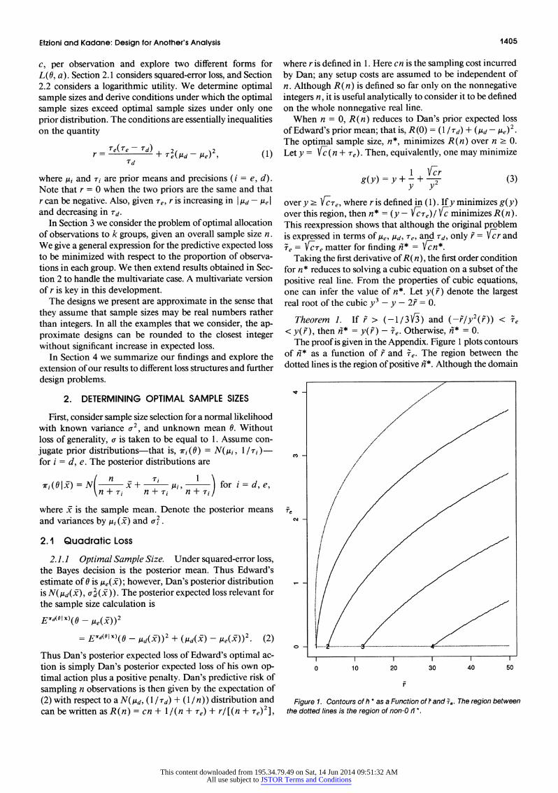
< y(f), then n* = y(F) - ) e. Otherwise, n1* = 0. The proof is given in the Appendix. Figure 1 plots contours

of n* as a function of F and Te. The region between the dotted lines is the region of positive n*. Although the domain

OV -

ciJ

I I I I I I

0 10 20 30 40 50

Figure 1. Contours of ih * as a Function of 7 and s.. The region between the dotted lines is the region of non-O fi*



1406 Journal of the American Statistical Association, December 1993

of r in Figure 1 extends to -1 /(31V/), the scale of r is so large that it appears that r extends only to 0. Several interesting aspects of the solution are revealed by this figure.

First, one can see the region in which the optimal value of n* is 0, toward the upper left of the figure. This corresponds to a region of large ITe (i.e., high prior precision on Edward's part) and small F(i.e., reasonable agreement between the two parties and high prior precision on Dan's part). The optimal sample size is also 0 when r is sufficiently negative; that is, when fd exceeds Te, Te is bounded away from 0, and the prior means are close. Under these circumstances, it may not be worth Dan's while to do the experiment. For example, in the extreme case of ageement between the two parties (r = 0), the prior precision, interpretable as a prior sample size, may be so high as to make sampling simply unnecessary. In this case, y(F) = y(O) = 1. From the theorem, if Te < 1, then n* = 1 - Te If ie ? 1, then n* = 0. Hence for Te > 1, it becomes optimal not to sample.

If Se iS fixed, then n-* increases with F. In other words, n* increases as the prior means diverge and/or Dan becomes less certain about his prior mean. This can be understood intuitively by viewing the two-prior problem as a one-prior problem in which Dan is attempting to sample optimally to estimate suboptimally. Edward's posterior mean is a sub- optimal estimate for Dan, but Dan can reduce his estimation penalty by bringing Edward's posterior mean close to his own. But doing so will require more observations, leading to higher sampling costs. For Dan, the crucial question is this: How many observations does he think he will need to bring the posterior means into reasonable agreement?

For fixed Te, the answer is a function of both the difference in prior means and Dan's prior precision. Certainly, prior means that are further apart will require more data to bring them together a posteriori. In addition, as Td gets smaller, Dan's predictive distribution becomes more diffuse about his prior mean; this increases the number of observations that he thinks he will need to bring Edward's posterior mean into reasonable agreement with his own. Hence the rela- tionship between r and n* in Figure 1. Note that Figure 1 cannot be used to inform about the behavior of n* as a function of r and Tie independently, as F is a function of Ee. In fact, F= Te{ (Te/Td)- 1 + (,ld -,e)2 }, so that as re , F 0, unless Td -)0 (or ( ,Ud

- e)2 00 ) at a rate greater than or equal to that of Te

The case Ie 0 is in fact of special interest, as many commonly used non-Bayesian inference rules coincide with Bayes estimates for a prior distribution with precision tending to 0. When Te - 0, F - 0 so long as I e- Ad I and Td are held fixed. By the preceding analysis, n-* -- 1, so n * -- 1 / Vc, which happens to be the optimal one-prior sample size under a flat prior. This suggests that if Edward's prior is diffuse, then Dan can well approximate the optimal sample size by designing as if he agreed with Edward.

2.1.2 Comparison With One-Prior Strategies. When Dan and Edward agree, the risk to Dan is R(n) = en + 1l/(n +r).If X < l/V9, then n* = (1/VP)--. Otherwise, n* = 0. In the two-prior problem, it is possible for one or both prior precisions to exceed the threshold 1 / i and to

still obtain a positive optimal sample size. In some cases the optimal two-prior sample size may be somewhat larger than the largest possible optimal sample size under one prior. For example, if c = .0625, then the optimal one-prior sample size is always less than or equal to 4, which corresponds to a prior precision of 0. But in the two-prior case, if I ,U- Pd I = 2, then n * is as high as 43 for Te = 6 and Trd = .01. Thus when ore is far from 0, two-prior sample sizes can be very different from the sample sizes that would be optimal for either prior distribution.

More formal statements about the difference between one- and two-prior optimal sample sizes can be made. Let ne*d

denote the optimal sample size for the problem in which 1re is used for estimation and Wd iS used for design ( ne*d = n* ). Then for fixed sampling costs, n*d 2 ne*,e if and only if r > 0. This is a direct consequence of the fact that y(r-) is nondecreasing in F (see the Appendix), and hence ne*,d is nondecreasing in r for fixed Te.

A special case of this result occurs when Dan and Edward have common prior means but different prior precisions. Suppose that Edward's prior is more precise than Dan's (Te

> Td). Then r is positive, and the optimal sample size for the experiment in which Edward estimates and Dan designs is greater than or equal to that for the experiment in which Edward both estimates and designs. The reverse is true when Dan's prior is more precise than Edward's. Note, however, that the condition -re > fTd is neither necessary nor sufficient for n * d to be greater than n *

2.2 The Loss Function -log(a)

Bernardo (1979) suggested the logarithmic utility function when the object of a study is to report the distribution of the parameter of interest (see also Lindley 1956). The development here is similar to that for squared-error loss. Edward's optimal decision is the a that minimizes -f 7re(I Lx)log(a) dO over the space of distributions on 0, and is given by a = ire( 61 X). The posterior expected loss relevant for the two- prior sample size calculation is -f Ird( 6 X)1)9log( ie(O 6X)) dO, and Dan's predictive expectation of this expression, plus sampling costs, can be written as

R(n) = cn + - log( 2

+ I

+ r

2 \fl+re/2 2(nl+T'e)

to be minimized over n. When n = 0,

2 ('Te ) 2 [Td+ ye]-

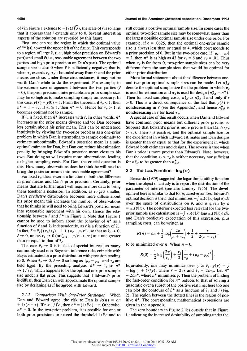
Equivalently, one may minimize over y 2 Te: g(y) = y -log y + (Fly), where F = 2cr and Te = 2Cre. Let n-* = 2cn*, where n * minimizes g. Then the problem of finding the first-order condition for n* reduces to that of solving a quadratic over a subset of the positive real line; here too one can plot the contours of n* as a function of Te and r (Fig. 2). The region between the dotted lines is the region of positive n*". The corresponding mathematical expressions are given in the Appendix.

The zero boundary in Figure 2 lies outside that in Figure 1, indicating the increased desirability of sampling under the




co

re

cIJ

0 10 20 30 40 50

Figure 2. Contours of n * as a function of h and ie: Logarithmic Utility. The region between the dotted lines is the region of non-O l*.

logarithmic loss. (But note the change in cost-normalization between squared-error loss and logarithmic loss.) Optimal sample sizes are higher under this loss structure than under quadratic loss, but they follow the same pattern for fixed fTe,

reaching their highest values when Dan's prior is relatively diffuse about a mean that conflicts with Edward's.

As -Te -- 0, the expected loss of not performing the experiment becomes infinite, while the optimal sample size and associated risk tend to a finite constant. Thus as Te tends to 0, it is always optimal for Dan to sample, and the optimal sample size is simply the one-prior sample size corresponding to Te = 0, namely 1/2c. Thus in this case too, Dan would do well to design in accordance with Edward's prior if Ed- ward's prior is diffuse.

Once again one can compare the optimal sample size when the two priors differ, to the optimal sample size under a common prior distribution, and the same result as in the quadratic loss case obtains. Fixing Edward's prior precision, n* > ne*, if and only if r> 0.

3. OPTIMAL ALLOCATION

This section examines the problem of optimal allocation of n observations to k groups, where n and k are given and the n observations y are independent and normally distrib- uted with common variance, which we take to be equal to 1 without loss of generality: y 10 N(XO, I).

Here 6 is a k vector of unknown group means, X is an n X k design matrix, and I is the identity matrix. In the one- way layout, X TX = diag { npi }; np, is the number of observations allocated to group i. Conjugate normal priors on 6 are 7ri (6) = N(gi, T`' ), i = d, e. The posterior distributions are normal with means i,t (y) = (Ti + XTX) A,( T1 + XTy), i = d, e, and precision matrices Ai = (T, + XTX), i = d, e. The goal is to solve for Dan's optimal allocations {pi } given that the estimate of 6 will be selected according to Edward's prior distribution. For instance, suppose (as in Smith and Verdinelli 1980) that the first group, with mean 01, corresponds to a control treatment, and Dan believes that the other treatment means are exchangeable, but not with the control. If Edward is skeptical and believes that all the groups are exchangeable, then gd = (M, A', Ai)

T

. , . . s~~~~~T T Td = diag{I-T, r', ... r', and Ae = (AL, A , 1) e

= diag IT, T, . * . IrJ

3.1 Quadratic Loss

Under the quadratic loss function L(6, a) = ( - a)T X (6 - a), Dan's posterior expected loss is

E 7rd(OIY)(6 - Ae( Y)) T(6 - ue(Y))

= tr(Ad ') + (.td(Y) - ge(Y)) T( Ad(Y) - Ae(Y))- (4)

Dan's predictive distribution on y is N(Xgd, I + XT-1l X T); the Appendix shows that Dan's predictive expectation of (4) is given by

R(n, p) = tr(Ae-1) + tr(Ae-7RA&-1), (5)

where R is a matrix version of r in (1): R = TeT-l(Te - Td) + Te(td - Ite)(Id - Ae)TTe. If Te = diag{r 1}, then Ae = diag { zi }, where zi = Ti + npi, and the optimization problem is to minimize g(z) = z (I/zi) + z (rii/z ) subject to the constraints z = z ri + n and zi ? Ti. This optimization problem is solved by setting equal to 0 the partial derivatives with respect to zi and X of the Lagrangian g(z) + X(E Zi -[ ri + n]) and then solving for zi 2 Ti and X. The values of z, and X thus obtained will be denoted X* and z*

In practice one may fix X equal to an initial value, Xo. Solve the equations obtained by equating the derivatives of the Lagrangian with respect to z, to 0. The solutions obtained will depend on X0 and are denoted z (X0). Then obtain an updated value for X by substituting the Z* (X o) into the equation obtained by equating the derivative of the Lagrangian with respect to X to 0. Iterate through these two steps until X converges. The computations are aided by the fact that for given X, the zi solutions are solutions to a cubic equation that is almost identical to that obtained in the optimal sample size problem. By similar arguments, one may derive conditions under which observations will be allocated to group i. These conditions are given in the Appendix, together with an argument that proves the existence and uniqueness of A*.

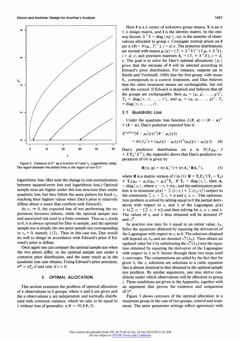
Figure 3 shows contours of the optimal allocation to a treatment group in the case of two groups, control and treatment. The prior parameter settings reflect agreement with




It -

CIT

l I I I l I

0 10 20 30 40 50

r22

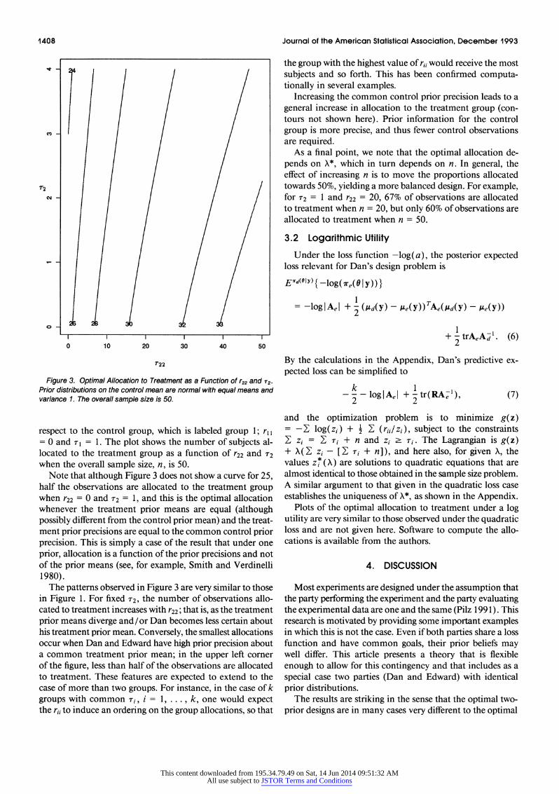
Figure 3. Optimal Allocation to Treatment as a Function of r22 and T2.

Prior distributions on the control mean are normal with equal means and variance 1. The overall sample size is 50.

respect to the control group, which is labeled group 1; r, I = 0 and -r1 = 1. The plot shows the number of subjects allocated to the treatment group as a function of r22 and T2 when the overall sample size, n, is 50.

Note that although Figure 3 does not show a curve for 25, half the observations are allocated to the treatment group when r22 = 0 and T2 = 1, and this is the optimal allocation whenever the treatment prior means are equal (although possibly different from the control prior mean) and the treatment prior precisions are equal to the common control prior precision. This is simply a case of the result that under one prior, allocation is a function of the prior precisions and not of the prior means (see, for example, Smith and Verdinelli 1980).

The patterns observed in Figure 3 are very similar to those in Figure 1. For fixed T2, the number of observations allocated to treatment increases with r22; that is, as the treatment prior means diverge and/or Dan becomes less certain about his treatment prior mean. Conversely, the smallest allocations occur when Dan and Edward have high prior precision about a common treatment prior mean; in the upper left corner of the figure, less than half of the observations are allocated to treatment. These features are expected to extend to the case of more than two groups. For instance, in the case of k groups with common Ti-, i = 1, . .., k, one would expect the rs1 to induce an ordering on the group allocations, so that

the group with the highest value of ri1 would receive the most subjects and so forth. This has been confirmed computa- tionally in several examples.

Increasing the common control prior precision leads to a general increase in allocation to the treatment group (contours not shown here). Prior information for the control group is more precise, and thus fewer control observations are required.

As a final point, we note that the optimal allocation depends on X*, which in turn depends on n. In general, the effect of increasing n is to move the proportions allocated towards 50%, yielding a more balanced design. For example, for r2 = 1 and r22 = 20, 67% of observations are allocated to treatment when n = 20, but only 60% of observations are allocated to treatment when n = 50.

3.2 Logarithmic Utility

Under the loss function -log(a), the posterior expected loss relevant for Dan's design problem is

E d( IY) { -lg(ire(O I Y))}

1 = -log Ael + - (/id(Y) - Ie(Y))TAe(Id(Y) - Ie(Y)) 2

+ trAeA-j1. (6) 2 ed

By the calculations in the Appendix, Dan's predictive expected loss can be simplified to

-2-loglAel + 2tr(RA-1), (7)

and the optimization problem is to minimize g(z) = -z log(zi) + 2 z (rii/zi), subject to the constraints

zi= i + n and zi 2 ri. The Lagrangian is g(z) + X( zi-[ - i + n]), and here also, for given X, the values z*(X) are solutions to quadratic equations that are almost identical to those obtained in the sample size problem. A similar argument to that given in the quadratic loss case establishes the uniqueness of X*, as shown in the Appendix.

Plots of the optimal allocation to treatment under a log utility are very similar to those observed under the quadratic loss and are not given here. Software to compute the allocations is available from the authors.

4. DISCUSSION

Most experiments are designed under the assumption that the party performing the experiment and the party evaluating the experimental data are one and the same (Pilz 199 1). This research is motivated by providing some important examples in which this is not the case. Even if both parties share a loss function and have common goals, their prior beliefs may well differ. This article presents a theory that is flexible enough to allow for this contingency and that includes as a special case two parties (Dan and Edward) with identical prior distributions.

The results are striking in the sense that the optimal two- prior designs are in many cases very diffierent to the optimal




one-prior designs. Optimal sample sizes (and allocations) are highest when Edward's prior is relatively peaked about a mean that contradicts Dan's prior mean, and they are lowest when Dan's prior is relatively peaked about a mean that agrees with Edward's. In the former case, the optimal sample sizes may greatly exceed the optimal one-prior sample sizes. The accompanying reduction in predictive risk leads us to conclude that in such extreme cases, if the person designing an experiment knows the prior distribution of the party evaluating the data, he would be wise to take it into account. For example, consider the case of squared-error loss with c = .0625. If Td = .01, re= 6, and lye - /dl = 2, then n* = 43, and Dan's corresponding predictive risk is 6.1. Given that Edward will be estimating, the predictive risk to Dan is 36 if he ignores Edward's prior opinion, and uses a sample size of 4 (one-prior optimum, corresponding to a prior precision of .01)-a six-fold increase! In practice, however, one would rarely expect to find such vague prior opinion on the part of the person designing (and paying for) the experiment. It is more common to have an estimation prior that is more diffuse than the design prior as in the legal and medical examples presented in Section 1. The results indicate that in these cases, optimal two-prior designs will not be too different from the optimal designs corresponding to the estimation prior; one would expect this to be true for other likelihoods as well.

This analysis leads to the question of whether the resulting designs are compromises in some sense, particularly for in- termediate values of the precision parameters. Lindley and Singpurwalla (1991) provided an example in which the optimal sample size in their adversarial problem falls between the two participants' optima, balancing the cost to the party performing the experiment of providing the data and the enthusiasm of the party evaluating the data for much of it. We have shown that in point estimation, the optimal two- prior sample size can exceed both one-prior sample sizes, but it may be interesting to examine conditions under which the optimal sample size falls between the individual optimal sample sizes.

Under a normal likelihood with known variance, is the extension from fixed sample sizes to sequential sampling as straightforward with two decision makers as with one decision maker? It is well known that with one decision maker having a normal likelihood with known variance, the optimal sequential sample size is equal to the optimal fixed sample size. But this is a result of the fact that in this case the posterior expected loss is independent of the sample data, at least for the loss functions considered in this article. With Dan and Edward, however, one must evaluate Dan's posterior expected loss of Edward's optimal action, which is not independent of the sample data. Thus the extension to sequential sampling seems to be nontrivial in the case of two decision makers.

Perhaps the most intriguing aspect of our development is the appearance of r as a critical quantity in the character- ization and evaluation of the optimal two-prior sample sizes, both in the univariate and in the multivariate cases. Can this quantity be interpreted as a measure of discrepancy between the two priors? Its asymmetry reflects the diffierent roles of

Dan and Edward in design and estimation, and it is certainly not a distance measure, but perhaps it might be calibrated to yield a meaningful measure of comparability of the prior distributions. An extension of this work would be to examine other likelihoods and loss functions to check whether r or some analog thereof plays a more extensive role than that already observed.

The work presented here is rich in potential extensions. For example, expressions (5) and (7) are quite general expressions in the sense that they hold for design matrices other than those implied by the one-way ANOVA and for nondiagonal prior covariance matrices. This suggests an extension to other design problems, such as linear regression. In the case of allocation problems, once the optimal allocation to k groups has been determined, it may be useful to consider the cost per observation, possibly different for different groups, and to solve for the optimal overall sample size n. The extension to other loss functions and likelihoods may not be straightforward, but we expect to see some similar results, and the work here should provide some useful guide- lines in these more-complex models.

We believe that experimental design is best modeled as a two-prior problem. We hope to see more two-prior designs in the future.

APPENDIX: PROOFS

Squared-Error Loss

Proof of Theorem 1. The cubic equation arises from differen- tiating g(y) with respect to y. By the properties of cubic equations (see, for example, Littlewood 1950), note that this equation has one real root if F< -(1 /3V3) or F> (1 /3V3), it has two real roots if r = -(1/3 Vi) or F = (1/31/i), and it has three real roots if - (1 /3 3) < r < (1 /3 3i). By studying the behavior of the function Y3 - y, one can ascertain whether the real roots of y3 - y = 2F = 0 are positive or negative. The function y3 - y decreases to -oo as y decreases to - oo, and it increases to oo as y increases to oo. It has a local maximum of (2/ 3 V3i) at y =-(1 / V3) and a local minimum of -(2/31V3) at y = 1/ V3i. Thus F <-(1 /3V3i) implies that y3 - y - 2F is nonnegative on y > 0. In this case g(y) is increasing in y for y > 0, and the optimal sample size is 0.

Similarly, if F > 0, then y3 -iy- 2F has only one positive root, which provides a local minimum, because g"(y) is nonnegative on y > 0 for F 2 0. Thus for F 2 0 there exists a unique, real,positive solution, y(F). The optimal sample size is (y(F) - e )/ c if y(Fr) > Te, and 0 otherwise. Note that F > 0 and y(F) > Te together imply that the second condition in the theorem is automatically satisfied.

Now consider the case -(1 (/ 31i) < F < 0, which has two positive roots. The smaller yields a local maximum; the larger yields a local minimum. The larger positive root is y(F). Is it sufficient to compare the values of re and y(F) when deciding on the optimal sample size? Because g(y) tends to -oo as y decreases to 0, it is not automatically true that g(y(F)) < g(Te) if y() > ie. In fact, for sufficiently small re, g(Te) may be less than g(y(F)). In this case the optimal sample size will be 0, not (y(F) - ie) /V7

For fixed F, and thus y(F), it is possible to obtain a closed-form expression for the values of ie such that g( fe) is less than g(y(F)). Clearly, if re is greater than or equal to y(Fr), then g(y) is increasing on [ fe, oo ), so that the optimal sample size is 0 in this case. Con- siderO0 < ie <y(F). There existsa t* such that ie t*~ g(ie) ? g(y(r)) n* = 0 and re > t* g(re) > g(yv(r)) n*




= (y(F) - ,e)/WI. Clearly, t* is a solution to the equation g(,e) = g(y(F)). This is a cubic equation in re, but it factors as (re - y(F))2(re + (r/y2(p))) = 0, indicating that the t* sought is t* = -[ly 2(r)] -

Conditions Necessary for Positive n*: -Log Loss

Under the loss function -log(a), the following result characterizes the optimal sample size n*. Let y(F) = (1 + V1 + 4F)/2. Let t*( F) be the solution of

t*- log(t*) + t* = g 2 ) if-4 < r < 0,

and t*( r) = 0 otherwise.

If F>-- and t*(F) < e<y(F), 4

then n* = y(r)- e; otherwise, n* = 0.

The reasoning here is similar to that under quadratic loss but somewhat more straightforward. This is due to the fact that y(F) is a solution to the quadratic equation 2 y - F = 0, which has roots (1 -) 2+4)2and(1 + I1+4F)/2.WhenF<-(1/4),the quadratic has no positive roots, and g(y) is increasing for positive y. When F> 0, there is only one positive root, and this provides a local minimum. When -(1/4) < F < 0, the quadratic has two positive roots. The smaller root is a local maximum; the larger is a local minimum. Because g(y) decreases to -oo as y tends to 0, there exists t*(F) for given r such that t*(F) E (0, (1- 1 + 4F)/2), and t* solves the equation

t*- log(t*) + g = g(l+ I +4)

Then

F, ' t* => g(,F,) ' g(Y(F)) =: nl* = O

and

re > t* * g(re) > g(y(F)) * * = y(F) -

The Multivariate Case: Quadratic Loss

Under the quadratic loss function L(O, y) = (0 - a) T( - a), the posterior expected loss relevant for the sample size calculation is

E d(O I Y)(O - Y)(y))(O - L(Y))

= tr(A-1) + (Itd(Y) - Ae(Y))T(Ad(Y) - Ae(Y))-

But (td(Y) - Ae(Y))T(Ad(Y) - ,e(Y)) can be expressed as

(Itd(Y) - Ae(Y))T(Ad(Y) - A (Y))

= (A-' - A-l )XT(X,Ad - y) + A 1Te(I(e - ttd). (A.1)

Using the symmetry of Ad, Ae, Td, and Te, and the fact that A`e - Aa1 = Aa- (Ad - Ae)Ae = Ad- (Td - Te)A -7, Dan's predictive expectation of (4) is

R(p) = tr(Ae-7[(A1 - Ae-l)XTX(T-lTe -I) + AeA-1])

+ tr(Ae-Te(Ate - td)(te -ATd)TTeAe-). (A.2)

This can be simplified using the following lemma.

Lemma. Let Z be an arbitrary conformable matrix. Then

tr Z[(Ad - -Ael)(XTX)(T-lTe -eI) + AeA

+ Te(siem-led)(ne -fld)lTeAei = tr(ZAe. R) + tr Z.

Proof Let S = tr(ZTe(ue - Ild)(I.le - ILdd)TTeAe). Then

tr(Z [(Ad-'l-A e-')(XTX)(Td-'Te -I) + AeAd-l]) + S

= tr(Z [Ad (XTXT -1Te _ XTX + Ae)1)

-tr(ZA `1XTX(T -,Te - I)) + S

= tr(Z [Ad-l(XTXT -1Te + Te)])

-tr(ZAe -(Ae - Te)(T -1Te - I)) + S

= tr(ZA -l(X TX + Td)Td ITe) - tr(ZTa ITe)

+ tr Z + tr(ZAe- R)

= tr(ZAa-TAdTa-TTe) - tr(ZTa-TTe) + tr Z + tr(ZAe-VR)

= tr Z + tr(ZAe -R).

This lemma is used with Z = Ae`1 in quadratic loss and with Z = I for -log d loss.

Conditions Necessary and Sufficient for Positive Allocation to Group i: Quadratic Loss

Given X > 0, let z(rij, X) denote the largest real root of the cubic, Xz3 - z - 2ri, = 0. If ri > -(1/3VX) and -(ri,/Xz2(X)) < Ti <z(ri,, X), then z* (X) = z(ri,, X); otherwise, Zi* (X) = Ti. This result is analogous to the univariate case.

Uniqueness of X

If X is negative, then the equation Xz3 - z - 2ri, = 0 does not have any positive roots for ri, > 0 and has a unique positive root, z(ri,, X), for negative ri,. But this root corresponds to a local maximum (in variable i) of the Lagrangian. Thus for X < 0, z* (X) = oo, and it suffices to consider only X 2 0. When X = 0, the problem reduces to a minimization of g(z) over the region { zi Ti 1 But note that ri, 2 -Ti so that g(z) 2 0 on this region [(Il/Zi) + (riilz2 ) 2 (Il/Zi) - (TiIZ2 ( llZi)(l- (TilZi)) 2 0]. Thus when X = 0, the optimal allocation to group i is infinite, and z 4(X) - T = oo. At the other extreme, when X = oo, we have z 4(X) - T < 0. This implies the existence of X satisfying

Z(XA) = Tri +n, (A.3)

which is the equation that results from equating to 0 the derivative of the Lagrangian with respect to X. This solution is in fact unique, as it is possible to show that for given R, z z (X) - T is decreasing in X for X > 0. We summarize the argument briefly as follows: For given ri, z(ri, X) is decreasing in X. Moreover, the region over which z4*(X) = z(ri, X) gets smaller as X increases, and the region over which z* (X) = ri gets larger as X increases. Consequently, z 4(X) decreases with X, and hence z z (X) - T decreases with

X. So X* is unique and positive and can be found quite easily, for instance, by a bisection algorithm.

The Multivariate Case: -Log Loss

Here the relevant posterior expected loss is a function of (/ld(Y) - Ae(Y))TAe(Ad(Y) - Ale(Y)). Using (A.1), Dan's predictive expectation of /.d(Y) - Sle(Y) is

EPd(Y)(,Ad(y) -Ae(Y)) = (I - A X TX)(Ae - AA

and the predictive variance-covariance matrix of ttd(Y) - Ite(Y) is

vPd(Y)(ZLd(y) - Ze(Y)) = (Ad1 - AeI)xTxTdilAd(Adi - Ae ).

Using a formula for the expected value of a quadratic form (Graybill 1976, p. 139), one can obtain the predictive expectation of (6). Some algebraic manipulation yields the following expression to be



Etzioni and Kadone: Design for Another's Analysis 1411

minimized over p,, i = 1, . . . k:

R(p) = -log I Ae I + 2 tr AeA d 2 e

+ I tr(A-j - A-l)XTX(T-lTe - I)

- - tr(le - ld) TeAe A e(Tee - ld) 2e

Compare this to (A.2). The preceding lemma yields (7).

Conditions Necessary for Positive Allocation to Group i: -Log Loss

Given X > 0, let wi = r1,/2, and let z(wi, X) = (1 + A1 + 4Xw )/2X. Let t*(wi, X) be the solution of

(Xt* - log(t*) + wi = g(l+ l I + 4Xw,)

if--I<w, <O, and t*(w,,X)=O 4X

otherwise. If w, > -(1/4X) and t*(w1, X) < r, < z(w1, X), then z (X) = z(w,, X); otherwise, z*(X) = T,

Here too, it suffices to consider only positive X by an argument similar to that given in the squared-error loss case. If X is negative, then XZ2 - Z- wi does not have any positive roots for w, > 0, and it is concave on { z, > Ti } for w, < 0. In fact, if X is negative, then z*(X) = oo. In the unconstrained problem (X = 0), we find also that z* (X) = oo, because wi 2 --ri/2. When X = +oo, z*(X) - T < 0, which proves the existence of a solution to (A.3) on the positive real line. The uniqueness argument mimics that for quadratic loss.

[Received February 1992. Revised October 1992.]

REFERENCES

Bernardo, J. M. (1979), "Expected Information as Expected Utility," The Annals of Statistics, 7, 686-690.

Burt, J. (1990), "Towards Agreement: Bayesian Experimental Design," Technical Report 90-41, Purdue University, Dept. of Statistics.

Chaloner, K., and Larntz, K. (1989), "Optimal Bayesian Design Applied to Logistic Regression Experiments," Journal of Statistical Planning and Inference, 21, 191-208.

DasGupta, A., and Studden, W. J. (1991), "Robust Experimental Designs in Normal Linear Models," The Annals of Statistics, 19, 1244-1256.

Graybill, F. A. (1983), Matrices with Applications in Statistics (2nd ed.), Belmont, CA: Wadsworth.

Jackson, P. H., Novick, M. R., and DeKeyrel, D. F. (1980), "Adversary Preposterior Analysis for Simple Parametric Models," in Bayesian Analysis in Econometrics and Statistics, ed. Arnold Zellner, Amsterdam: North- Holland, pp. 113-132.

Kadane, J. B. (1990), "Statistical Analysis of Adverse Impact on Employer Decisions," Journal oftheAmerican StatisticalAssociation, 85, 925-933.

Kadane, J. B., and Seidenfeld, T. (1989), "Randomization in a Bayesian Perspective," Journal of Statistical Planning and Inference, 25, 329-345.

Lindley, D. V. (1956), "On a Measure of Information Provided by an Ex- periment," Annals of Mathematical Statistics, 27, 986-1005.

Lindley, D. V., and Singpurwalla, N. (1991), "On the Evidence Needed to Reach Agreed Action Between Adversaries With Application to Accep- tance Sampling," Journal of the American Statistical Association, 86, 933-937.

Littlewood, D. E. (1950), A University Algebra, London: Heinemann. Pilz, J. (1991), Bayesian Estimation and Experimental Design in Linear

Models, Chichester, U.K.: John Wiley. Shannon, C. E. (1948), "A Mathematical Theory of Communication," Bell

System Technical Journal, 27, 379-423, 623-656. Smith, A. F. M., and Verdinelli, I. (1980), "A Note on Bayes Designs for

Inference Using a Hierarchical Linear Model," Biometrika, 67, 613-619. Spiegelhalter, D. J., and Freedman, L. S. (1988), "Bayesian Approaches to

Clinical Trials," in Bayesian Statistics 3, eds. J. M. Bernardo, M. H. DeGroot, D. V. Lindley, and A. F. M. Smith, Oxford, U.K.: Oxford University Press.

Tsutakawa, R. K. (1972), "Design of Experiment for Bioassay," Journal of the American Statistical Association, 67, 584-590.



Documents

Optimal Experimental Design for Another's Analysis