PAMM · Proc. Appl. Math. Mech. 16, 673 – 674 (2016) / DOI 10.1002/pamm.201610325

Optimal Experimental Design to Identify the Average Stress-StrainResponse in Short Fiber-Reinforced Plastics

Felix Ospald1,∗ and Roland Herzog1

1 TU Chemnitz, Faculty of Mathematics, 09107 Chemnitz, Germany

We show how to use optimal experimental design methods for the parameter identification of short fiber reinforced plastic(SFRP) materials. The experimental data is given by computer simulations of representative volume elements (RVE) of theSFRP material. The experiments are designed such that a minimal number of RVE simulations is required and that the modelresponse attains a minimal variance for a class of strains and fiber orientations.

c© 2016 Wiley-VCH Verlag GmbH & Co. KGaA, Weinheim

1 Modeling of SFRP Materials

The governing constitutive law of an SFRP material in the linear elastic case is derived by the so-called averaging procedureof Tucker [1] applied to the the constitutive law of a unidirectional composite (transversely anisotropic in the fiber direction):

Csfrp(c, A) : ε = c1ε+ c2 tr(ε) I + c3 (A tr(ε) + (A : ε) I) + c4(A ε+ εA) + c5 A : ε , (1)

where A is the second and A is the fourth moment of the fiber orientation distribution. In order to keep the dimensionalityof the problem reasonable, we compute A from the second moment A using the ORW3 closure [2]. The parameter vectorc := (c1, . . . , c5)T contains material constants, which depend on the material parameters of the fiber and matrix material, aswell as the volume fraction and aspect-ratio of the fibers.

2 Parameter Identification Problem

Given the average stresses σi := 〈σεi〉 ∈ Sym(3), i = 1, . . . , nexp of nexp experiments (RVE simulations), each performedwith the prescribed average strain εi and the moments of the fiber orientation distribution Ai the goal is to identify theparameter vector c in (1) which minimizes the sum of squared residuals

s(c) :=1

2

nexp∑i=1

‖Csfrp(c, Ai) : εi − σi‖2F −→ min . (2)

An optimal solution of this least-squares problem satisfies the normal equation

I c = JT y with I := JTJ ∈ R5×5.

I denotes the Fisher information matrix and J denotes the Jacobian of the residual in (2). y is a vector containing thevectorized experimental data σi. A priori it is not clear how to choose the design variables εi and Ai as well as the number ofexperiments nexp such that I becomes positive definite and, in a sense, as large as possible. Computing the complete stiffnessmatrix first and then identifying the parameters from there is possible (c.f. [3]), however this is a rather costly procedure.

3 Optimal Experimental Design Problem

Due to the discrete nature of computer experiments, the vector of experimental data y usually contains errors, which donot change if we perform exactly the same experiment again. However, the experimental setup (defined through the designvariables Ai, εi) determines the amplification of these errors in the determined parameters c. Since the sign and magnitude ofthese errors is a priori not known, we assume that each component of y contains random errors and that y follows a multivariateGaussian distribution y ∼ N (y, Σy) with mean value y and covariance Σy . The variance of the parameters is then given byΣc := σ2

y I−1. And the variance of the model response (evaluated and averaged over all possible rank one strains of unity

norm and rank one fiber orientation moments) is given by

Σy = σ2yW I

−1 with W =1

15

15 15 10 10 315 45 30 10 510 30 34 16 810 10 16 16 63 5 8 6 3

.

∗ Corresponding author: e-mail felix.ospald@mathematik.tu-chemnitz.de, phone +49 (0)371 531 33498, fax +49 (0)371 531 833498

c© 2016 Wiley-VCH Verlag GmbH & Co. KGaA, Weinheim

674 Section 15: Applied stochastics

Design I (nexp = 1, f(A1, ε1) = 3.050) Design II (nexp = 2, f(A1,A2, ε1, ε2) = 1.574)

A1 = diag(0.7545, 0.2455, 0) A1 = A2 = diag(1, 0, 0)

ε1 =

(0.1095 0.3644 −0.22240.3644 0.2551 −0.3601

−0.2224 −0.3601 0.5467

)ε1 =

(0.6105 −0.3953 0.2582

−0.3953 0.1630 −0.10780.2582 −0.1078 −0.3628

), ε2 =

(0.5990 −0.1589 0.3623

−0.1589 0.2584 0.13190.3623 0.1319 0.4745

)

Table 1: Table of optimal design solutions.

0 0.2 0.4 0.6 0.8 10

0.2

0.4

0.6

0.8

1

a1

a2

Design I

4

6

8

10

0 0.2 0.4 0.6 0.8 10

0.2

0.4

0.6

0.8

1

a1

a2

Design II

1.6

1.7

1.8

1.9

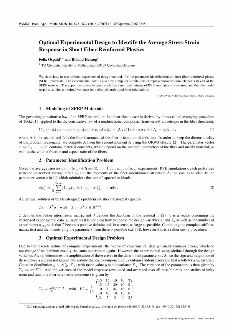
Fig. 1: Plot of the objective function for varying A1 = diag(a1, a2, a3) with a3 = 1 − a1 − a2 at fixed (optimal) ε1, ε2 and A2. Theoptimal solutions are shown as magenta bullet (•). The constraint a1 ≥ a2 ≥ a3 is shown as white triangle.

The goal of our optimal design is to minimize the mean variance of y (i.e., the trace of Σy) w.r.t. the design variables, i.e.,

minεi∈G,Ai∈H∀i=1,...,nexp

log(nexp tr(Σy)

)︸ ︷︷ ︸=:f(Ai,εi)

, where G := {ε ∈ Sym(3) : ‖ε‖F = 1} andH :=

{diag(a) : a ∈ R3, a1 ≥ a2 ≥ a3 ≥ 0, a1 + a2 + a3 = 1

}.

(3)

The mean variance of the model response is then given by 13nexp

exp(f(Ai, εi)), which is proportional to σ2y .

4 Numerical Results and Conclusions

The solutions of (3) for nexp = 1, 2 are given in Table 1. For Design I we have rank(A1) = 2, i.e., a planar fiber distributionturns out to be optimal. Design II requires two experiments with unidirectional fiber orientations (rank(Ai) = 1). The rank 1solutions are generally more favorable as they allow more densely packed fibers and more efficient/simple computations aswell as experimental setups (i.e., for tensile specimens). When we use the quadratic closure instead of the ORW3 closure noparameter identification is possible in case nexp = 1. For Design II the quadratic and ORW3 closure are equivalent.

The plot of the objective function for varying A1 = diag(a1, a2, a3) with a3 = 1 − a1 − a2 at fixed (optimal) ε1, ε2 andA2, shown in Figure 1, reveals the choices of A1 for which no parameter identification is possible due to a rank-deficientJacobian J . For Design I this is the case if one eigenvalue of A1 has a multiplicity of 2. For Design II, a variation of A1 hasonly small influence on the objective, so it can be chosen more or less arbitrarily. Looking at Figure 1 it seems that there aremultiple local minimizers. However, since we restricted the moments to the triangle a1 ≥ a2 ≥ a3, these symmetric solutionsdisappear and there is only one solution for A1 and A2. The optimal Ai imply certain symmetries for ε, which do not changethe objective. Therefore all optimal solutions are global optimal.

Further experiments revealed that Design II is a robust choice for the parameter identification. For nexp > 2 the designsare clustering (due the assumption of uncorrelated noise) and do not reduce the optimal objective function value any further.More details are available in the preprint [4], submitted to CMAME.

Acknowledgements This work was performed within the Federal Cluster of Excellence EXC 1075 “MERGE Technologies for Multifunc-tional Lightweight Structures” and supported by the German Research Foundation (DFG). Financial support is gratefully acknowledged.

References[1] C. Tucker and S. G. Advani, Journal of Rheology 31 (1987).[2] D. H. Chung and T. H. Kwon, Polymer Composites 22(5), 636–649 (2001).[3] A. Gusev, M. Heggli, H. Lusti, and P. Hine, Advanced Engineering Materials 4(12), 931–933 (2002).[4] R. Herzog and F. Ospald, Optimal experimental design for linear elastic model parameter identification of injection molded short

fiber-reinforced plastics, Tech. rep., TU Chemnitz, submitted.c© 2016 Wiley-VCH Verlag GmbH & Co. KGaA, Weinheim www.gamm-proceedings.com