Optimal Prime-Time Television Network Scheduling

Reddy, S.K., Aronson, J.E. & Stam, A.

IIASA Working Paper

WP-95-084

August 1995

Reddy SK, Aronson JE, & Stam A (1995). Optimal Prime­Time Television Network Scheduling. IIASA Working Paper. IIASA, Laxenburg, Austria: WP­95­084 Copyright © 1995 by the author(s). http://pure.iiasa.ac.at/id/eprint/4512/ 

Working Papers on work of the International Institute for Applied Systems Analysis receive only limited review. Views or 

opinions expressed herein do not necessarily represent those of the Institute, its National Member Organizations, or other organizations supporting the work. All rights reserved. Permission to make digital or hard copies of all or part of this work 

for personal or classroom use is granted without fee provided that copies are not made or distributed for profit or commercial advantage. All copies must bear this notice and the full citation on the first page. For other purposes, to republish, to post on servers or to redistribute to lists, permission must be sought by contacting repository@iiasa.ac.at 

Working Paper Optimal Prime-Time Television

Network Scheduling

Srinivas K. Reddy Jay E. Aronson Antonie Stam

WP-95-084 August 1995

IVIIASA International Institute for Applied Systems Analysis A-2361 Laxenburg Austria

kd: Telephone: +43 2236 807 Fax: +43 2236 71313 E-Mail: info@iiasa.ac.at

Optimal Prime-Time Television Network Scheduling

Srinivas K. Reddy Jay E. Aronson Antonie Stam

WP-95-084 August 1995

Working Papers are interim reports on work of the International Institute for Applied Systems Analysis and have received only limited review. Views or opinions expressed herein do not necessarily represent those of the Institute, its National Member Organizations, or other organizations supporting the work.

VllASA International Institute for Applied Systems Analysis A-2361 Laxenburg Austria

.L A.

..MI. Telephone: +43 2236 807 Fax: +43 2236 71313 E-Mail: infoQiiasa.ac.at

Foreword

Many practical decision problems have more than one aspect with a high complexity. Current decision support methodologies do not provide standard tools for handling such combined complexities. The present paper shows that it is really possible to find good approaches for such problems by treating the case of scheduling programs for a television network. In this scheduling problem one finds a combination of types of complexities which is quite common, namely, the basic process to be scheduled is complex, but also the preference structure is complex and the data related to the preference have to esti- mated. The paper demonstrates a balanced and practical approach for this combination of complexities. It is very likely that a similiar approach would work for several other problems.

OPTIMAL PRIME-TIME TELEVISION NETWORK SCHEDULING

Srinivas K. Reddyl

Jay E. Aronson2

Antonie Stam2y3

1: Department of Marketing, Terry College of Business

The University of Georgia, Athens, GA 30602, U.S.A.

2: Department of Management, Terry College of Business

The University of Georgia, Athens, GA 30602, U.S.A.

3: MDA Project, International Institute for Applied Systems Analysis

A-2361 Laxenburg, Austria

Optimal Prime-Time Television Network Scheduling

ABSTRACT

This paper introduces SPOT (Scheduling of Programs Optimally for Television), an analytical

model for optimal prime-time TV program scheduling. Due in part to the advent of new cable TV

channels. the competition for viewer ratings has intensified substantially in recent years, and the

revenues of the major networks have not kept pace with the costs of the programs. As profit margins

decrease, the networks seek to improve their viewer ratings with innovative scheduling strategies. Our

SPOT models for scheduling network programs combine predicted ratings for different combinations

of prime-time schedules with 3 novel, mixed-integer, generalized network flow, mathematical

programming model, which. when solved, provides an optimal schedule. In addition to historical

performance, subjective inputs from actual network managers were used as input to the network flow

optimization model. The optimization model is flexible. It can utilize the managers' input and

maximize profit (instead of ratings) by considering not only the revenue potential but also the costs

of the shows. Moreover, SPOT can describe the scheduling problem over any time period (e.g.. day,

week month, season), and designate certain shows to, and restrict them from. given time slots. The

methodology of SPOT is illustrated using data obtained from a cable network during the first quarter

of 1990. The optimization model produces solutions which would have generated an increase of

approximately 2 percent in overall profitability, representing over $12 million annually for a typical

network with an average Nielsen rating of 18. SPOT not only produces more profitable TV schedules

for this network, but also provides valuable general insights into the development of mixed

programming strategies for improving future schedules.

Optimal Prime-Time Television Network Scheduling

1. INTRODUCTION

In the last decade, the television indusuy in the U.S. has seen tremendous changes which have

dramatically affected its operations. Not too long ago, the three major networks (ABC, CBS and NE3C)

routinely captured over ninety percent of the viewing audience during prime-time, but in recent years

their combined share has decreased to about sixty percent of the viewers. Meanwhile, network

program costs escalated from about $200,000 for an hour of prime-time in 1971 to over $1 million

today, For example, in 1991 NE3C ordered the ninth season of Night Court at $1.5 million for each

of the 22 half-hour episodes for the 1991-1992 season. Hence. as costs have increased and

competition stiffened, the profitability of prime-time programming has declined.

The advertising revenues of the TV networks are linked directly to the size of the audience

delivered to the advertiser. The number of viewers of a show is measured using ratings provided by

the old Nielsen meters or the new Peoplemeters (Webster and Lichty 1991. p. 17). With billions of

dollars being spent on TV advemsing, and $9.6 billion spent on network TV advertising in 1989

alone, a swing of only one rating point translates into a loss or gain of millions of dollars in

advertising revenues for the network. The outlook in terms of the total viewing audience is not very

encouraging for the three major networks. as their average ratings are gradually shrinking. Krugman

and Rust (1987) expect this trend to continue, projecting the combined ratings of the major networks

to fall to about fifty-four percent by the year 2000.

In sum. the competitive ratings arena has essentially become a game where the gain of one

network could mean big losses for another '. There has never been a more urgent need to schedule

prime-time TV prognms carefully to maximize the network's ratings or profits. To complicate the

scheduling task, the success or failure of a given show not only depends on the contents,

characteristics. and cost of that show, but also on the show against wtuch it is placed.

' Ted Danzig, the Editor of Advertising Age in an interview on McNeil-Lehrer Newshour. September 1989.

Though little published information exists on the use of analytical models to aid scheduling

in the television industry, there has been some pioneering work in the management science literature

on scheduling models using ratings data by Gensch and Shaman (1980). Horen (1980) and Henry

and Rime (1984a. 1984b); and the research by Rust and Echambadi (1989), which uses individual

level viewing choice data. The current work attempts to extend this body of research by presenting

SPOT (Scheduling of Programs Optimally for Television), analytical models for optimal prime-time

TV program scheduling. These models combine predicted ratings with a novel, mixed-integer,

generalized network-based flow, mathematical programming model, to provide an optimal schedule.

Apart from the unique network flow-based model, SPOT is flexible in that it can utilize the managers'

expert inputs, and can maximize profit (instead of just TV ratings), by considering not only the

revenue potential, but also the costs of the shows. The models are illustrated using data obtained

from a cable network.

The remainder of the paper is organized as follows. In Section 2, we review the literature on

scheduling strategies and models. and summarize the contributions of our research. In Section 3, the

SPOT methodology is introduced and justified. including both regression-based and judgmental data

estimation, and the mathematical programming, network-based flow model used in SPOT to assign

shows to time slots. The results of applying SPOT to a cable TV network and a discussion of model

validation issues are presented in Section 4, followed by computational tests in Section 5 and potential

model extensions in Section 6. The paper ends with a summary and conclusions in Section 7.

2. LITERATURE REVIEW

2.1. Scheduling Strategies

Among the most commonly used scheduling strategies is the "lead-in" placement strategy

which relies on the strength of the preceding prognm to boost the ratings of a newly introduced, or a

weaker program, following it. Empirical evidence supporting such a strategy has been reported in the

pioneering work by Ehrenberg and Goodhardt (1969). Goodhardt and Ehrenberg (1969) and

Goodhardt, Ehrenberg and Collins (1975). Further evidence confirming the effectiveness of a lead-

in scheduling strategy has been found by Headen, Klompmaker and Rust (1979). Henry and Rime

(1984), Horen (1980), Tiedge and Ksobiech (1986) and Webster (1985). A variant of the lead-in

strategy considers the carry-over effects of sequences of more than two programs. The lead-in effect

of one program can be viewed as the "lead-out" effect of the previous program. Taking the lead-in

lead-out effects of three consecutive programs is often called a "hammocking" or "sandwiching"

strategy.

Ganu and Zohoori (1982) found that viewers appear willing to structure their lives around

television preferences, and that viewing behavior is sensitive to changes in the television schedule.

Their study identified the time at which the show is aired and the contents of the prognm as the most

important factors affecting TV viewers' behavior. Hence, a television station's program schedule has a

critical impact on the type and the size of the audience it attracts, and the task of designing an

effective schedule is a crucial component of a network programmer's responsibility. The i programmer must not only acquire an inventory of programs, but also design a weekly schedule

which places the available shows in the appropriate time slots in a manner which attracts as large an

audience as possible. Head (1985, p. 27) describes the task of scheduling the programs of a station,

cable or network as " ... a singularly difficult process." Read (1976, p. 72) refers to broadcast

television scheduling as an "arcane, crafty, and indeed. crucial" operation. With the increasingly

rapid changes that are shaping the indusuy, scheduling has become more crucial and challenging

today than at any time in the past.

It is not surprising that Michael Dann, a veteran network program executive and consultant,

stated that "... where a show is placed is infinitely more important than the content of the show." (New

York Times, February 26, 1989, p. 42). Therefore, it appears that optimal prime-time program

scheduling is a powerful and important means for networks to realize an acceptable profit level.

2 2 . Scheduling Models

There is little published evidence that formal and systematic approaches are used to guide this

process. Rather, network programmers often rely on heuristics and subjective judgments. The

program scheduling task as currently practiced appears to draw largely on past experience, instinct

and guesswork. Stipp and Schiavone (1990) report that to gather information about how to best

schedule their programs, NBC asks potential viewers whether they would watch a particular show if it

were aired at the same time slots as competitors' shows. This kind of scheduling research technique is

usually referred to as "competitives." The information from sample surveys and viewer

questionnaires is then used to implement a scheduling strategy aimed at attaining high ratings.

Analytical research on scheduling network programs includes the work based on aggregate

ratings data by Gensch and Shaman (1980). Horen (1980) and Henry and Rime (1984). and the

research by Rust and Echambadi (1989). using individual level viewing choice data. Gensch and

Shaman (1980) use a trigonometric time-series approach to predict ag,gegate audience viewing for

different days, times and seasons. The predicted audience values are then used to develop four

different network share models to apportion the total market share of the three major television

networks. Each of these network share models is based on specific assumptions about the suength of

program loyalties, and the manner in which TV viewers form viewing preferences. Even though their

model only takes into account the seasonality of the time-series data and does not consider the

content of the program itself, Gensch and Shaman's (1980) predictions are highly accurate. Based on

the findings of Gensch and Shaman (1980). Rust and Alpert (1984) hypothesize that television

viewing may be conceptualized as a two-stage choice process: in the first stage the individual decides

whether or not to watch TV, and in the second stage selects which program to watch.

Several approaches have been proposed to model this second stage of viewing choice

behavior at the individual level. Rust (1986) provides a comprehensive review of viewing choice

models. Using an economic utility approach. Lehrnann (1971) relates program type and production

quality to preference for television shows. Dannon (1976) uses both channel loyalty and program

type to predict individual viewing choice. Zufryden (1973) views program selection as a dynamic

process, and uses a linear learning model formulation in which the current choice behavior is a

function of previous viewing choice decisions.

To date, the most comprehensive individual viewing choice model proposed is Rust and

Alpert's (1984) audience flow model. This research uses Luce's (1959) choice axiom to estimate

utilities for television prognms based on segment-wise preferences for program type and audience

flow. "Audience flow" records include data regarding the status of the TV set, in addition to

infomation on whether the set is on or off at a gven time. whether the TV remains tuned to the same

channel during a given program. and whether the program is ongoing or just starting. Rust and

Alpen (1984) found the audience flow model very accurate in predicting individual viewing choices,

with correct predictions about 76 percent of the time.

Henry and Rinne (1984) investigate the effectiveness of several commonly used scheduling

strategies such as "blunting" and "counterprograrnming," and suggest several options for scheduling

programs during the week in relation to the competit i~n.~ However, the Henry and Rime study does

not provide a model or method that can be used to schedule television programs.

Rust and Echambadi (1989) develop a heuristic method for scheduling a television network's

programs. Their approach differs from the previous methods, in that they explicitly incorporate

individual viewing choice by extending the audience flow model developed by Rust and Alpert

(1984). Their heuristic. which maximizes the nerwork's share of audience. produces program

schedules, with substantially improved viewership over the original schedules. The flexibility of the

model permits one to use an objective function other than audience share, and consider managerial

constraints like slotting a particular show for a particular time or having certain programs appear only

after 9:OO p.m.

Gensch and Shaman (1980) strongly suggest that models whlch incorporate expert opinions

should be developed. The insights of practitioners in areas such as audience demographics, program

content and competition should be extremely critical in determining not only the accuracy but also

the successful implementation of those models.

Horen (1980) provides an explicit two-stage model to develop program schedules. This

model defines multiple, half-hour program segments. Longer shows are divided into "program-

' Horen (1980) defines the "counterprogramming" strategy as scheduling programs in a given time slot which are of a different type than the programs offered by the competing networks in that time slot. A network using this strategy would place a show that appeals to one specific audience (say. women between the ages of 18-45) against a competing network's program which is aimed at a different audience (for example. men between the ages of 45-60). "Blunting." is the opposite of counterprogramming. A network applying this strategy seeks to schedule "strength against strength." offering a program with similar or greater appeal to the same target audience as its competitor's program at a given time slot. Tiedge and Ksobiech (1987) found that in the past, counterp~ograrnming has been used more widely than blunting. Based on an analysis of prime-time programs in the period 1963-1984, they found that pure blunting was used only 1.4 percent of the time, while pure counterprogramrning accounted for over 60 percent of the scheduling strategies.

Page 6

parts," with ratings detailed for each program-pan. In the first stage, Horen (1980) uses past rating

information of the three major TV networks to predict ratings for each class of programs and each

prime time slot by means of linear regression. In the second stage, a mathematical programming

model is used to determine a potential schedule which maximizes the ratings.

However, a schedule which simply maximizes ratings may not be optimal for the network.

The costs of shows differ dramatically, and as a result, it is possible that inexpensive shows are highly

profitable, even though their ratings are lower than those of other more costly shows.3 In SPOT, we

take into account both the revenues and costs associated with each show, providing a more accurate

indicator of the show's contribution to the network's profit. LMoreover, SPOT will address the

hypothesis that by using historical data or ratings for the existing schedule, an expert can better

estimate how well a show will fare in each time slot. Judgmental estimates by experts may very well

be more accurate than those found through forecasting by regression.

The contribution of this paper is the introduction of a novel, flexible, network-based flow

model that analytically describes the difficult problem of scheduling of television programs

optimally. We demonstrate that this approach is superior to that proposed by Horen (1980) in terms

of computational effort and flexibility of the schedules. The flexibility of SPOT is demonstrated by

its ability to incorporate show costs and revenues, rather than simply ratings, to incorporate either

regression forecasts or expert judgments, the ability to assign certain shows to and restrict others from

specific time slots, and the ability to handle lead-in effects directly.

3. METHODOLOGY OF SPOT

3.1. ~Modeiing Framework

The modeling fnmework of SPOT is based in part on the work of Horen (1980). The basic

assumptions made in Horen's mathematical programming model are (1) other networks' schedules

' Several recent repons in the media suggest that some networks do use a suategy to maximize profit. The placement of a low cost news feanue 48 Hours by CBS against the immensely successful. but expensive The Cosby Show of NBC is a prime example. Other networks are trying similar strategies. illustrating that with escalating program cosw. maximizing ratings may no longer be optimal. ABC was the only one of the three major networks to earn a profit during 1991-92 season, even though it ranked h d based on Nielsen's ratings. Its success is mainly amibuted to a strategy of programming and scheduling shows to maximize profit rather than just ratings (Business Week April 20. 1992). Hence. it appexs useful to build a scheduling model which considers the profit potential of each show at my rime slot

remain fixed. and (2) the network's objective is to maximize its total expected ratings. Horen's model

is a generalization of the classical assignment model. but it is neither a pure network nor a generalized

network flow problem. Some of the shows last more than one program part (one half-hour),

necessitating the use of complicating constraints which require combinatorial problem solving

methods. Further. Horen does not explicitly address a variety of desired model features, such as.

having more show durations than the time slots allow, assigning of a particular show to a particular

time slot; assigning of a set of shows to a set of time slots; assigning of a sequence of shows to a set

of time slots and restricting shows from certain time slots. The lead-in effects are approximated by

linear costs to avoid a quadratic objective function.

Similar to Horen (1980). the modeling framework of SPOT consists of two stages. The first

stage uses either a regression model based on past profit data (from past ratings and costs of shows)

(for SPOT-REG), or a judgmental analysis (for SPOT-EC) to predict the potential performance of

each show at alternative time slots. Predictor variables in the regression model include show type,

duration of the show, relative attractiveness of the show, day and time the show is televised.

In SPOT-EC, the Analytic Hierarchy Process (AHP) is used to obtain the manager's

judgments or assessments of the relative importance of each of the critical variables. This results in

relative performance values for each combination of show and time slot, which in turn serve as a

prediction of how well a particular show would do at each particular time slot. In the process of

determining the judgmental forecasts, the manager has access to the past performance data of each

show.

The advantage of incorporating judgmental factors is that i t enables one to explicitly consider

qualitative and conceptual factors which may affect program ratings. It may be difficult o r

impossible to include such factors in a regression modeling framework. By offering the option of

using either regression or judgmental inputs, SPOT provides considerably greater flexibility than

previous modeling efforts. It also provides an opportunity to compare these two approaches, and, as

discussed in Section 4.2, determine which appears to give more accurate rating predictions. The

regression forecasting model and judgmental forecasting model are discussed in more detail in

Sections 3.3 and 3.3, respectively.

Page 8

The projections from either the SPOT-REG or the SPOT-EC analysis are then used as inputs

into the second stage of SPOT. In this stage, a generalized. mixed-integer. network-based flow model

is used to determine the optimal prognm schedule given the inputs from the first stage. The general

modeling process is outlined in Figure 1. The model components of stage 2 are discussed in detail in

Section 3.5.

................................. Figures 1 and 2 About Here

3.2. Data

The data used were provided by a major cable network, and represent actual programming

utilized by this network during the first quarter of 1990. For confidentiality, this cable network is not

identified and the data are disguised, but the numbers are representative. Each week during this

quarter (for 13 weeks), the network aired 26 different half-hour and hour-long shows in the 8-11

p.m. prime-time period, LMonday through Sunday. The data provide information on show

characteristics, each show's relative attractiveness to the network's audience, as measured by the

manager's judgment,' the cost of each show, each show's 'Tlr ratings, and the cost per thousand (CPM)

charged to the advertisers for commercial time during each show.

On average, during this quarter, there were I 0 half-hour shows, 1 6 hour shows of 6 show

types to fill the 42 half-hours of prime-time slots every week. Using the data, our regression model

was employed to predict net profit objective values for the allowable combinations of shows and time

slots. Based on our discussion with the Program Director, the following assumptions were made:

1. The model encompasses half-hour time slots from 8:00 p.m. to 1 I :00 p.m., over a l l seven

days of the week.

2. Shows have durations of one half-hour (I program-part) or one hour ( 2 program parts).

3. Two program-part shows may only start at 88:00,9:00 or 1O:OO p.m.

'The Program Director at the network was asked to evaluate each show that was telecast during the first qu;ata of 1990 in tams of its perceived attractiveness to the audience on 1 to 10 scale. with 10 being most attractive and 1 being least artractive. Eliciring evaluations post-hoc poses some potential concerns in terms of memory and accuracy. However. similar judgments have been used by Dacin and Smith (1994). Reddy, Holak and Bhar (1994) and Smith and Park (1992).

3. The seven best shows, as identified by the network manager, are one hour in length. and must be scheduled at 9:OO p.m., every night.'

5. Lead-in effects are negligible.

In consultation with the network managers. the shows are classified into six homogeneous

types. based on their general characteristics. These show types are identified by the following

symbols: A, H. L, N . P and S. The full description of these categories is not given to maintain

confidentiality. A typical week's schedule of the network during the first quarter of 1990 is presented

in Figure 2.

Before proceeding with the forecasting model used to predict viewer ratings, the general

relationships between the revenues during the first quarter of 1990 and sevenl key show

characteristics are presented graphically in Figure 3.

................................. Figure 3 About Here

Figure 3 indicates that for this cable network, the H and S type shows tend to perform the best

in generating revenues. Moreover. hour-long shows do substantially better than half-hour programs.

Tuesdays and Saturdays are the best days in terms of revenues. whle the 9:00 p.m. and 1O:OO p.m.

time slots tend to generate more revenues than other prime-time slots.

As discussed above. the SPOT profit forecasts can be estimated in two ways. Initially. we

present SPOT-REG. followed by an outline of SPOT-EC.

33. Regression Forecasts (SPOT-REG)

At the aggregate level. regression models have been used in the past in forecasting TV ratings.

Horen (1980) uses a linear regression model but did not explicitly incorporate characteristics of the

television shows. Henry and Rime (1984a) use a logit model to predict ratings with show

characteristics as predictors of ratings, but do not address the issue of optimal scheduling of television

' As 9.00 p.m. slot is the most desirable prime-time slot. the besr shows with the greatest audience appeal and potentially highest ratings are scheduled at this time slot. Seven shows were identified as fulfilling these requirements by the Program Director.

shows. Neither of these models dealt with the issue of cost of shows. We propose a richer. aggregate

forecasting model which not only explicitly incorporates the show characteristics, day and time

characteristics. but also managerial perceptions of the relative attractiveness of each of the television

shows.

1 where Yit is the rating of show i in time slot r , Ai is a measure of the relative perceived attractiveness

of show i of type 1, measured on a ten point scale, while S; . D: and are zero-one variables

which equal one if. and only if, show i is of type j, scheduled on day k (Monday through Sunday), in

time slot m (half-hour slot between 8 and lor30 p.m.), respectively. The binary variable R: equals

zero if, and only if, the duration of show i is one half-hour, and one if the show lasts one full hour,

and Eit is the residual term.

The time-series data on 26 shows over 13 weeks were pooled to estimate the model presented

here. Pooling of this data may be considered a problem if the shows may be considered a source of

heterogeneity. As we are using show and day and time characteristic variables in the model for the

differences, pooling is not a concern (Parsons and Vanden Abeele 1981). However, the Lagrange

Multiplier (LM) test (Breusch and Pagan 1979) indicates the presence of heteroskedasticity. As a

result, applying ordinary least squares (OLS) will produce unbiased but inefficient estimates (Belsley

1973), necessitating the use of the generalized least squares (GLS) procedure (Greene 1993; Draper

and Smith 1981; Montgomery and Peck 1982) to estimate the model. More details on the effects of

using different estimation procedures on the outcomes of the SPOT and Horen models are discussed

in Section 5.

The model estimates using both OLS and GLS are presented in Table 1. The explanatory

power of the model is good, as reflected by an adjusted R2 of 0.926 and 0.943 for OLS and GLS,

respectively. Perceived show attractiveness is positive and significant, indicating it to be strong

determinant of ratings and, in turn, on revenue. Show duration is also positive and significant. so that

one-hour shows generate significantly more revenue per half hour than half-hour shows. Overall, as

expected the GLS procedure provides a slightly better R2 and the parameter estimates have smaller

Page 1 1

standard errors. The current model is only a main effects model. and some intenction effects could

be added to improve the predictions. However, adding selected interaction terms to the model

improved the only margin all^.^ In other contexts. if the main effects do not predict well. it may be

necessary to include intenction terms selectively. This, and other model validation issues, will be

addressed in Section 5. Other enhancements could be made to the model, for instance by including

audience characteristics. The estimates from this model are used to project revenues for shows at

various time slots, and as inputs into the optimization component of SPOT-REG.

--------------------------------- Table 1 About Here

3.4. Judgmental Forecasts (SPOT-EC)

The utilization of management science models by managers is limited in practice. Alluding to

the lack of application of these models, Little (1970, B466) describes the practice as "... a pallid

picture of promise." identifyin2 the absence of communicarion between manager and model as the

key element for such lack of implementation. The attempt here, in developing a judgmental model, is

to involve the manager directly in the modeling process by asking for hisher expert inputs. Thus, the

manager is an integral part of the model. This is achieved by incorporating managers' judgments on

the relative importance of the various aspects of the TV shows (e.g.. show type, show attractiveness.

duration, time of day, day of the week, etc.), to generate forecasts which can supplement and validate

the regression forecasts discussed in the previous section. In addition to getting management directly

involved in the process. judgmental forecasts also reflect aspects of the decision problem which

cannot be captured by the quantitative information used in obtaining regression forecasts.

Judgmental estimates of the relative importance of assigning shows to certain time slots can be

obtained using any preference elicitation method, as long as the resulting importance measures are

based on a ratio scale. In SPOT-EC, the "absolute judgment" mode of the Expert Choice (1992)

software implementation of the Analytic Hierarchy Process (AHP) developed by Thomas Saaty

For example, of the 30 show type x day interactions. only 10 were s i f i cu l~ with an increase in the adjusted R* to .935 in the cue of OLS and to 0.946 in the case of GLS. Moreover, the addition of these interactions has caused a severe collinearity problem. As the main effects model has accounted for a substanrid variance, and due to the problems caused by multicollinearity, interaction terns were nor included.

(1980. 1986) is used for this purpose. The relative importance judgments can be based on revenue

and profit, but it is also possible to include other relevant factors. The AHP has recently emerged as

an extremely useful tool in analyzing complex business decision problems, and has proven

particularly helpful in determining priority scores and preference rankings of the decision

alternatives. Applications of the AHP in combination with optimization techniques include general

mathematical programming (Bard 1986; Harker 1986; Liberatore 1987; Stam and Kuula 1991), and

network analysis (Sinuany-Stem 1984). The AHP has also been applied successfully in marketing,

notably by Wind and Douglas (1981) and Wind and Saaty (1980).

For sevenl reasons, we have opted to use the absolute judgment approach of the AHP in

SPOT-EC, rather than the relative judgment mode, in order to avoid the rank reversal problem in the

AHP (Dyer 1990a, 1990b). because it facilitates an easier evaluation of large numbers of program

combinations, and because the analysis and evaluation of new shows is straightforward. Note that, in

contrast. it may be difficult to accurately predict profits or TV ratings for new shows using any

regression-based model, because no "hard" historical data exist on these shows. In the A H . analysis,

no such hard data are needed; only the manager's subjective judgments.

Therefore, the absolute judgment approach of the AHP appears to have potential advantages

over the regression based approach, and should certainly prove useful to the network program

scheduler as an additional decision support tool. Since SPOT-EC yields ratio scale results, these can

serve as the input - in the same way as regression estimates - into the network-based flow model

analysis, which, as described in Section 3.5, determines the optimal scheduling of shows to time slots.

........................................ Figure 4 and Table 2 About Here ........................................

In Figure 4, we show an AHP hierarchy with the five factors (criteria) that affect the profit

contribution of each program-time slot combination: show type, show attractiveness. day of the week,

time slot, and show duration. The numerical values in the figure reflect the relative importance

judgments of the criteria and of the different categories for each criterion made by the network

scheduling expert. In our case. the expert judged each of the five factors equally important in terms

of impact on profit. implying weights of 0.20. which need not be the case in general. Table 2

illusuates the ovenll relative importance of twelve different representative show assignments

(alternatives 01 through 12) to various time slots and days-of-the-week for our example. Once the

suucture of the scoring spreadsheet in Table 2 has been set up, it is easy for the manager to evaluate

any combination of show-time slot assignment, existing or new, by selecting the appropriate

categories of the five factors.

33. Generalized Network Flow model for TV Scheduling

We now discuss stage 2 of the SPOT methodology: the development of a mixed-integer,

generalized network flow model that accurately describes the 'I7 scheduling problem structure. A

network is a graphical representation of a flow problem. By defining the problem as a network, it can

be visualized and stated mathematically, facilitating model and problem analysis, efficient solution,

managerial understanding and more readily acceptance of the problem by non-analysts. In fact, pure

network flow problems can be solved up to 100 to 200 times faster by network programming

algorithm implementations than by standard linear programming ones (Aronson 1989). Generalized

network flow problems can be solved 10 to 20 times faster than by standard linear programming

methods. Mainly due to compact, graphical problem representation and optimization procedures,

network algorithms can solve much larger problems than can be solved by more general optimization

techniques.

We adopt the definition of integer, one half-hour "prognm-parts" for shows longer than one

half-hour (Horen 1980). A complication for atl TV scheduling models is that shows extend over

multiple, consecutive time slots, which destroys the pure network structure of the model. The

program-parts determine values of arc multipliers for our generalized network structure to enforce

these conditions. In addition, we introduce some simple side constraints to speed up the optimization

substantially. The simultaneous treatment in SPOT of both half-hour and hour or longer shows within

a network-based flow formulation is a novel modeling contribution.

The model is related to that of an assignment problem with some intermediate nodes and arcs

with multipliers. The supply-to-demand arcs indicate the scheduling of a single program-part show.

Page 14

In SPOT-REG, their arc objective values are the individual show's estimated net profit defined by

profit = revenue - cosr; in SPOT-EC. the individual show's estimated scores based on managerial

experience obtained through the AHP. If required, it is possible to use show ratings. The supplies to

intermediate node arcs indicate scheduling a multiple program-part show. Its multiplier equals the

number of half-hour program-parts of the show. The intermediate node to demand arcs split the

multiple program-parts of shows into the requisite. consecutive half-hour time slots. We next

introduce the notation and terminology necessary to describe the mathematical formulation of the

network flow problem.

Let N be the set of nodes and A the set of arcs consisting of ordered pairs of nodes (i, I), i, j E

N. The network is defined by [ N . A]. Let N: c N be the set of "to" nodes j E N for which (i. 1) E

A. and N; c N the set of "from' nodes i E N for which (i. j) E A. With each arc (i, j), we associate a

flow xij, a conuibution to the objective function per unit flow cij, a multiplier qj, a flow capacity uu.

and a lower bound of zero.

Furthermore, let K be the maximum number of program-parts of all shows under

consideration, denote the set of all supply nodes corresponding to K program part shows (k = 1 for

half-hour shows. k = 2 for hour shows. ere.). by sk, k = 1, ..., K; lk be the set of intermediate nodes for

time slots of k program-part durations. for k = 2, ..... K; and let demand node Tj represent the j-th

time slot to be filled for j = 1. ,,., J.

The time slot nodes are grouped into set T. The show nodes are supplies that have

requirements of +I, the intermediate nodes are transshipment nodes. and the time slot nodes are

demands with requirements of -1. To balance the network to enforce feasibility, if the number of

program-parts (P) exceeds the number of time slots to be filled (D), a dummy demand node (Td )

having requirement - (P - D) is added to the network. If D > P. then a dummy show. corresponding

to unknown television shows to be added into the line-up at a later date, with a requirement of D - P

program-parts is added. To match the shows with appropriate, consecutive time slots, a rime slot group

G~ is defined as a set of sets of consecutive time slots that may be filled by a show with a duration of

k prognm-parts. k = 2, ..., K. There is equal flow through each of the arcs in such a time-slot group.

which requires a simple side constraint set to be included in the problem.

The integer, generalized network-based flow SPOT TV scheduling model may be described

as:

K K

(I) Maximize z = z z cs X, + z z c i , , , xi,,, + z z z c , xi , ( 2 )

subject to:

x u E {O, 11, (i, j) E A. (9)

The first term of (2) represents the contribution to the objective of the half-hour shows; the

second term is for the half-hour show arcs linked to the dummy node; the third term is for the

multiple time slot shows. Constraints (3)-(7) are the conservation of flow consuaints. Constraint set

(8) tightens the linear programming relaxation. forcing equal flow on the arcs fmm intermediate to

time slot nodes. There are only I Gk I -1 such constraints for every set Gk. Constnint set (9) enforces

the binary condition on all arcs. Because the requirements of the supplies are all +I , the multipliers

are defined by show duration. and the demand node requirements are all -1, so that no explicit

Page 16

statement of arc flow capacities is needed; the model defaults to a 0. I (binary) problem. See Figure

5 for the graphical representation of an example problem.

Figure 5 About Here

The SPOT integer, generalized network flow model is a difficult, NP-hard (Nemhauser and

Woolsey 1988) combinatorial problem. However, if all shows and time slots have equal duration, o r

if certain other simplifications occur (e.g., all half hour shows are of the same type and quality), then

SPOT becomes an easily solved, pure assignment problem. Though this rarely occurs in practice, the

SPOT model describing the third quarter data of 1990 for the cable network was transformed into a

pure assignment problem. The SPOT model, when solved. provides an optimal schedule given the

profit projections based on either inputs from SPOT-FZEG or SPOT-EC. It is possible just to use TV

audience rating estimates. but, as previously noted, there is a weakness when show costs are not

included. High ratings for an expensive show may not be as desirable as lower ratings for a modestly

priced show in terms of the contribution to the overall net profitability of the television network.

Further, a schedule that maximizes net profit also maximizes ratings but not vice versa.

3.6. Lad-in Effects

Lead-in effects complicate the structure of the generalized network somewhat, introducing

either nonlinearities or approximations in the objective function as in Horen (1980), which leads to a

quadntic cost function. or by including additional, non-network side constraints. Let x u represent

the assignment of show i to a time slot or intermediate node j; let xpq represent the assignment of

show p to the next available time slot or intermediate node q ; and let cipj represent the pairwise

conuibution to the objective when show i starting in time slot j precedes show p in the next starting

time slot q . Then the quadratic term Cipj xu xpq must be included in the objective (2) for every

relevant pair of shows in every relevant pair of consecutive time slots. The model then becomes

related to the quadratic assignment problem (see Aronson 1986). However, the foLlowing set of side

constraints and additional linear objective function terms can be introduced to avoid creating a

nonlinear, integer programming problem:

- 5 O.S(xij + xpq ), al l relevant (i, j), (p . q) assignments, -!PI (10)

:ipj I xu + xpq - 1, all relevant (i, j), (p, q) assignments. (1 1)

zip, E (0, 1 ) . (12)

The linear term tip, zip, is added to the objective (2) for every relevant pair of shows in every

relevant pair of consecutive time slots. See Aronson and Klein (1989) and Klein and Aronson (1991)

for a similar modification to a model describing MIS development. Aronson and Klein (1989) and

Klein and Aronson (1991) implicitly bundle the constraints into precedence definitions in an implicit

enumeration method. Since we are interested in solving (1) - (9) directly for TV scheduling, (10) -

(12) can be used explicitly. As long as there are only a few pairs of shows for which lead-in is

important, these side constraints will prove effe~tive.~ If there are many, then data estimation for each

pair of shows in each time slot may prove difficult, if not impossible to perform.

Unul now, no one has attempted to explicitly define lead-in directly and accurately into their

scheduling models, probably due to its complexity. The novel approach of Aronson and Klein

(1989) and Klein and Aronson (1991). though not well known in the scheduling literature. produces

an exact, linear, but complex, characterization of lead-in effects.

4. RESULTS

Figure 5 illustrates the network-flow representation of our example problem, taken from the

weekly prime-time schedule for the first quarter of 1990 provided by the Program Director of the

cable television network. The existing set of shows and the network-based flow model defined in (I)

were used to determine optimal schedules for different objective functions.

Specialized methods can be developed for solving SPOT. However, typically more than 10%

of the SPOT model rows are non-network due to the presence of a mixture of one-hour and half-

hour shows (or other show lengths), it is ineffective to use an integer, generalized network with side

constraints code (see Aronson 1989). In several computational experiments, comparing the

specialized integer, generalized network with side constraints code developed by Adolphson (1989)

According to the Program Director of the cable network. only a limited number of pairs of shows' lead-in effects must be typically considered among othen because many of the revenue or ratings estimates would not be sufficiently accurate.

Page 18

with the computationally robust Linear INteractive. and Discrete Optimizer, HyperLINDO (Schrage

1991a, 1991b). we found that for the particular type of problem in our application, HyperLINDO

yielded faster and more accurate solutions, on average. None of the problems took over 2 seconds to

solve. Therefore, in our analysis we used HyperLINDO on an IBM PC compatible computer with an

Intel 80486 processor at 66 MHz. In our tern, we omitted lead-in effects. We used net profit OLS

(NO) and GLS (NG) estimates from the regression formula (1) to generate weekly SPOT models for

the first quarter of 1990. We further tested models with ratings generated from OLS (RO) and GLS

(RG) regression formulas. and an AHP / Expert Choice (EC) generated model. For each of these five

models, three progressively tighter cases are investigated: (1) restrict the time slots at 9:00 p.m. to

any of the hour-long shows; (2) restrict the time slots at 9:00 p.m. to only the seven best hour-long

shows on any given day; and (3) fix the schedule so that the seven best hour-long shows are

scheduled at 9:00 p.m. on their given days in the actual schedule for the first quarter of 1990. We

also substitute the Base or actual schedule solution into each objective function category, yielding the

objective value of the actual schedule. We shall call this Case 4.

For Case 1. the complete SPOT network model has a total of 76 nodes and 14 side

constraints. Of the 798 arcs or variables, only 644 arcs are used because only hour-long shows may

be scheduled at 9:00 p.m. By back substitution of the variables in the side constraints, the problem

size was reduced to 76 rows and 630 variables. of which 336 are explicitly declared as integer. For

Case 2, further arc elimination yielded a problem size of 76 rows and 469 columns (175 integer). For

Case 3, the problem size could be reduced further to 62 rows and 420 columns (120 integer).

4.1 SPOT-REG Results - Net Profit (NO and NG)

The weekly net profit of the actual Base solution appears in Table 3 for comparative

purposes. AU computational runs took less than two CPU seconds to solve. The objective values

found for all twenty cases, and the value of the Base schedule are shown in Table 3a. Table 3b

indicates the difference (degradation) from the optimal value.

......................... Table 3 About Here

From Table 3a. we see that the weekly operating cost, revenue and net profit for the Base

schedule are $3,180,000, $9,500,310 and $6,320.3 10 respectively.

The objective values of the net profit models (NO and NG) progressively degrade as the

models become more resuictive. Consider column 1 (NO), for the Net Profit SPOT models with

objective coefficients generated from OLS. The optimal NO solution (with a profit of $6,448,263)

only scheduled 4 of the best shows at 9:00 p.m., and none on their designated days as in the Base

schedule. When the restriction that only the best hour shows are allowed to be scheduled at 9:00 p.m.

(Case 2). still none of the best shows were scheduled on the same day as in the Base schedule. The

objective value of Case 2 dropped slightly from the optimal value of $6,448,263, by a mere $197 per

week (only $10,244 per yex) or 0.003%, to $6,448,066. In Case 3, for which the best shows are

locked into their respective days and rime slots, the objective value degrades by $21.288 or 0.330%,

to $6,426,975. m e Case 3 optimal solution is $1 19,799 or 1.858% better than Case 4, the Base

schedule using the regression coefficients. Finally, the optimal solution yields net profits that are

about 2% higher ($127,953) than the Base schedule.

The increase in net profit for Case 1 and Case 2 over the Base schedule may initially not

appex to be much of an improvement, but one should remember that this increase in profit is

obtained without incurring any additional costs. On an annual basis this increase translates to over

$12 million, in higher net profit for a big 3 network with a Nielsen rating of about 18 which is

substantial in an industry where the profit margins are dwindling due to increased competition.'

Similar SPOT regression models developed for the second and third quarter data for 1990 yielded

comparable results.

Interestingly, the optimal solution for the first quarter data props up weak second half-hour

time slots, especially in the 10:30 time slot, by always scheduling one hour shows at the 10:00 time

slot. In each of the Case 1-3 model solutions, all of the 10 half-hour shows were scheduled at 8:00

and 8:30 p.m. All of the Net Profit OLS (NO) schedules used Monday and Saturday as the evenings

to schedule one-hour shows at 8:00 p.m., boosting ratings at 8:30, while the NG schedules used the

a Cumulative profirs of the three major networks which were a healthy $800 million in 1984 shrunk to St00 million by 1988 (Auletta 199 1).

Page 20

one-hour shows on Thursday and Friday evenings. See Figure 6 for a revenue breakdown by time

slot and day.

................................. Figures 6 and 7 About Here

Inspecting past data. it was evident that the 10:30 p.m. slot is indeed weak. By scheduling a

half-hour show at 10:OO p.m., the audience is given an option to turn off the television or switch to

some other channel. By scheduling an hour-long show at 10:00 p.m., the network is able to hold on

to a larger portion of the audience. This is precisely the strategy that the Program Director followed

for the second and third quarters of 1990. The optimal solutions also verified the Program Director's

opinion about which seven of the shows were the best (most profitable) to air fmm 9:00 - 10:OO p.m.,

since the optimal Case 2 net pmfit solution for the NO model degraded by only $197 per week.

Compared with the Base schedule (Figure 2), the schedule obtained through SPOT (Figure 7)

improves the profit at the weaker time slot (10:00 p.m.) and on the weaker days (certainly for

Wednesday, Thursday and Friday). Further, the use of the 8:00 and 8:30 p.m. time slots for aIl the

half-hour shows indicates a trade-off between propping up the 10:30 time slots and maintaining

audience early in the evening. This redistribution of profit illustrates that the model maximizes the

schedule over the entire week. rather than concentrating on any particular time slot, or day.

Comparable results are obtained for the Net Profit GLS model (NG). When moving from the

optimum (Case 1) to Case 2, the objective value decreases by $1229 (.019%) per week, whereas the

decrease for Cases 3 and 4 are 0.364% and 1.730%. respectively. The percentage difference between

the Base Case solution for the NG model is somewhat less than that for the NO model, 1.348%

($86,378 per week). The number of the best shows that are scheduled at 9:00 p.m. for Case 1 is 2.

with none on their designated days, whlch is worse than the 4 shows scheduled for the NO schedule.

For NG Case 2, none of the best shows were scheduled on their designated days. The fact that

moving from Case 1 to Case 2 results in only a minimal decrease in the objective value for both the

NO and NG models indicates that the Program Director's opinion on which shows were the seven best

is fairly accurate.

For both the OLS and GLS Net Pmfit models. the increased profit over the Base solution

exceeds $600,000 per week, or over $6.2 million per year.

Page 2 1

1.3 SPOT-REG Results - Ratings (RO and RG)

We modified the regression formula (1) to produce weekly ratings estimates, on a half-hour

basis, to a SPOT model. The ratings models, RO for OLS and RG for GLS, were designed to

maximize the total weekly ratings for the network, considering one-half hour ratings values per time

slot, and were also solved by HyperLINDO. The results are reported in Tables 3a and 3b.

Interestingly, Cases 1 - 3 have the same objective value each for the RO and RG models; the objective

function value did not degrade as the problem became more resuictive. Thus, the 7 best shows yield

the highest ratings when restricted by time slot and by day. In a l l 6 models, the 10:OO p.m. time slot

contained only one-hour shows, again propping up the 10:30 time slot, but the days for which the

8:00 p.m. time slot contained one-hour shows varied, depending upon whether or not a %st' show

was available to boost the ratings. It should be noted that a ratings maximization approach is

equivalent to maximizing revenues, so that more options exist to boost weak half-hour time slots with

hour shows than in the case of maximizing net profit. The Base schedule regression objective value

degraded from that of the optimum ntings models (Case 1) by 0.679% for the RO model and

0.623% for the RG model. This translates to a ratings boost of over 0.6% per week (on avenge, for

every half-hour time slot) for simply shuffling the weekly prime-time line-up. The ratings models

also varied more widely than the net profit models. in terms of the evenings at which a one-hour show

was scheduled in the 8:00 p.m. time slot.

4.3 SPOT-EC Results - AHP / Expert Choice

The use of expert judgmental forecasts on the show portfolio for the first quarter of 1990 are

next examined. We set up the AHP I Expert Choice scoring method as described in Section 3.4. and

shown in Figure 4. The scores resulting from the preference analysis are used as objective function

coefficients of the SPOT-EC model. The optimal objective function value of 23.140 (in Table 3a)

represents the sum of AHP scores associated with show-time combinations selected in the optimal

schedule shown in Figure 8. Cases 2 and 3 yielded solutions for which the objective values were near-

optimal (see Tables 3a and 3b), When using the AHP / Expert Choice relative importance coefficients,

the Base solution (Case 4) had an objective value of 22.913 which was 0.981% worse than the

Page 22

optimum. However, the results for the AHP /Expert Choice (EC) model solutions are better than

those for the Net Profit OLS solutions, and comparable to those of the Net Profit GLS schedules. The

objective value percentage decrease from the optimum to the Base solution is a bit less than the net

profit GLS case. As for the NO and NG models, some improvement (about 1%) can be attained over

the Base schedule by simply rescheduling the existing line up. In Case 1. the EC models scheduled

one-hour shows at 8:00 p.m. on Wednesday and Friday; in Case 2 on Wednesday and Thursday; and

in Case 3 on Wednesday and Saturday.

Figure 8 About Here .........................

It is interesting that in Case 1, EC selected 5 out of the 7 best shows to be scheduled at 9:00

p.m.. with 1 on the same day as the Base solution. In comparison, the NO optimum selected only 4,

with none on their designated days; the NG Case 1 solution selected only 2 of the best shows, and

neither on their Base schedule day; RO used 2 and RG used 3 of the best shows at 9:00 p.m. in their

respective Case 1 solutions. Thus. we found that the EC solutions best reflected the Prognm Director's

preferences in the placement of the 7 best shows. This result is not surprising, in that the Program

Director's judgment was used in developing the objective function coefficients.

4.4 Comparison of SPOT Model Results

Summarizing the scheduling aspects of the various models, the identification and fixed

scheduling of the 7 best shows did not impact severely upon the objective value for the optimal

schedule obtained for each model. However. scheduling half-hour shows during the relatively weak

10:30 p.m. time slot does. The common factor of a l l models was that the optimal schedules did prop

up the relatively weak 10:30 p.m. time slots by scheduling only hour-long shows at 10:OO p.m. all

week. The Base schedule has half-hour shows during the Wednesday through Friday 10:OO and

10:30 p.m. time slots. and during the Monday and Wednesday 8:00 and 8:30 p.m. time slots.

Inspecting the various optimal schedules in detail, we found that for two days per week. all schedules

filled the 8:00 p.m. - 9:00 p.m. slot with a one-hour show, considering the 8:30 p.m. time slot a write-

off.

Page 23

The EC optimal schedule had more (5) of the best hour-long shows scheduled at 9:00 p.m.,

and one on its designated day, followed by the NO model with 4 at 9:Ml p.m.. none on its designated

day, while for NG these figures were 2 and 0. Though not a net profit optimizer, the EC model best

captured the Program Director's judgments about which he considered to be his best shows. In terms

of the two net profit models, the EC solution yielded objective values that were within 0.893% of the

optimum objective value for NO; and within 0.901% for NG, both comparable to the results of the

RO and RG ratings models.

It is also interesting to analyze how each model's optimal schedule and the Base schedule

compare when using the objective function measures of the other models. In Table 4a, we show a

cross comparison of the objective values corresponding to the six weekly SPOT models: Base, NO,

NG, RO, RG and EC. There is a row and column corresponding to each of the six models. In the first

column, we show the objective values of the Base schedule. For the remaining columns, the diagonal

element is the objective value to its optimal Case 1 SPOT schedule (corresponding to the least

restrictive models), shown in Table 3. In each column. of the first row, Base, we show the objective

value obtained when inserting the Base schedule directly into the column's model's objective function

(NO through EC), i.e., the value of the actual schedule, using the regression-generated coefficients.

The objective values in rows 2 through 6 are found by inserting the model row's optimal schedule

into the column's model. For example, inserting the optimal schedule found when solving the ratings

GLS (RG) model (row 5, column 5). into the objective function of the net profit GLS (NG) model

yields the value of 6,374,944 in row 5 , column 3

We validate the model by first considering the direct improvement of the weekly Net Profit

models over the Base (actual) schedule. As a baseline measure, we observe from Table 4a that the NO

objective with the Base solution is only $8,154 (0.129%) larger than the Base solution value of

$6,320,310. while for NG model, the value is less by only $24,427 (0.386%). Based on this small

variation, the generated objective function coefficients of the models are reasonable estimates.

Similar results hold for the ntings models. We cannot compare the base schedule data to AHP 1

Expert Choice model, but the confirmatory evidence presented earlier indicates consistency with the

Program Director's judgments.

Page 24

Furthermore, Table 4a shows that the Case 1 optimal solution to the NO model is $127,953

(2.024%) larger than that of the Base solution, while the optimal NO solution in the NG model yields

a weekly increase in objective value of 578,559 (1.243%). When considering the other situation, the

optimal NG solution was $86.378 (1.367%) larger than the Base schedule's weekly value, and

substituting it into the NO model, we obtain a weekly increase in net profit of $113,674 (1.799%).

Regardless of which of the two net profit optimal solutions we choose, we obtain a minimum increase

in weekly net profit of over 1.2% per week, simply by rescheduling the shows. The ratings and EC

model optima, when substituted into the Net Profit models, increase the weekly objective function

value by between 1.1 % to 1.4%. translating to between $1.5 and 53.6 million per year.

For the remainder of our comparisons in this section, we shall use the regression estimates for

the Base schedule. In Tables 3b and 4c, we show the improvement in the objective value over the

Base schedule. In all cases, the optimal solution increase ranges from just under 1%. to about 2%.

......................... Table 3 About Here

Consider the Net Profit OLS model. The net profit models are most sensitive to the different

optimal schedules. They do yield optimal ratings. However, the non-optimal ratings models do not

yield optimal net protits (or overalI revenue). That is to say, both net profit models. both ratings

models and the EC model schedules, when substituted into both of the ntings models (RO and RG)

yield optimal ntings values. However. each ratings model's optimal solution. when applied to both of

the net profit models (NO and NG) yield sub-optimal solutions for which the objective is still better

than that of the base schedule. For the EC model. the other optimal model schedules yield objective

values that are slightly worse (about 0.22 or 0.960%) than that of the base schedule (22.913). while

the optimum EC schedule is 0.991% or 0.227 better than that of the base schedule value of 23.140.

The optimal NO model value of $6,448,263 is $1 19,799 or 1.893% better than the value of

the weekly base schedule of $6,328,464. The NG optimal schedule produces change in the objective

value within 5% of the change due to using the optimal NO schedule. Even the two optimal ratings

and the AHP / Expert Choice schedules improve the net profit (NO) by between 0.996 and 1.289%

over the base schedule. Comparable results are obtained for the NG model.

Page 25

The results for the EC values are consistent with the Program Director's opinions and with the

results obtained from the net profit regression-based objective. The consistency of the solutions and

their objective values found by using both expertise and regression confirm the validity of the final

schedule and adds credence to the application of our network-based analytical approach.

5. COMPUTATIONAL STUDY

In this section, we study the extent to which the regression models are robust with respect to

variation in the data. Additionally, we analyze the impact of this variability on the results of the SPOT

and Horen optimization models, both in t e n s of net profit and computational performance. Weekly

fluctuations in the viewershp, as reflected by the ratings, offer a challenge to the programming

executive. Typically, over a quarter. our TV network has experienced a variation in ratings of about

five percent. Wide variation in ratings may influence the regression estimates, and as a consequence

may affect the results of the optimization. potentially leading to sub-optimal program schedules.

Another issue of interest is to investigate how the model estimates are affected by heteroskedasticity

in the data. To this purpose, we estimate all of the models using ordinary least squares (OLS) and

generalized least squares (GLS) procedures. GLS takes into account the presence of

heteroskedasticity, whle the simpler OLS is preferred if the data are homoskedastic.

As the actual variance in ratings during the Fall 1990 quarter was about five percent about the

mean show ratings, we conduct Monte-Carlo simulation experiments with 2, 5 , and 10 percent

variation in ratings, reflecting the low, moderate and high end of ratings fluctuations. Each data

condition is replicated 10 times. so that the total number of data sets generated is 30, the number of

regression models ro be estimated is 60 (30 OLS and 30 GLS models), and the number of

optimization runs is 120 (60 each for SPOT and Horen). Obviously, the typical fluctuations may be

different for other applications. Moreover, in general the fluctuations may differ by show, but we

chose ro vary the ratings uniformly across all shows. This simulation design wdl provide us with the

magnitude of effects and a general sense of direction due to variation in the ratings.

5.1 Parameter Estimates

The summary of OLS and GLS regression parameter estimates for different degrees of rating

variation is presented in Table 5. As one would expect, the predictive power of the model as reflected

Page 26

by the ~2 improves with lower variability in ratings. Models with only 2% variation have an ~2 of

about 96%. whch is about 3-12% higher. on avenge. than the 10% variation models. That the

explanatory power of GLS models appears to be slightly worje than the OLS models. Very few o f

the OLS and GLS parameter estimates differed substantially, as indicated by the root mean squared

difference computed for each set of estimates.

...................................... Tables 5, 6a and 6b About Here ......................................

The OLS and GLS estimates were used as input into SPOT and Horen's model. Three key

performance measures of output from SPOT and Horen's model are monitored -- computational

performance, as measured by CPU time and number of pivots: and solution quality, as measured by

predicted net profit (or ratings).' Table 6a provides the mean performance measures and their

standard deviations. for SPOT and Horen model, when optimizing for net profit. Table 6b provides

the corresponding resulrs when optimizing for ratings. Obviously, as both SPOT and Horen's model

solve to optirnaiity, these methods will always yield identical predicted net profit (ratings) figures

when using the same objective function values. However, the results presented in Table 6 suggest that

in all cases, SPOT outperforms Horen's model in terms of solution time and pivot count. The average

improvement of SPOT over Horen ranges from 2548% in CPU solution time, and from 37-5356 in

pivot count.

3-2 Effects on iModel Choice

Analysis of variance was used to ascertain whether the optimization model (SPOT and Horen),

the estimation procedure (OLS and GLS) and the variance in ratings (2%. 5%. and 10%) significantly

affect the three key measures of performance. Tables 7a and 7b provide the ANOVA results when

optimizing for net profit and ratings, respectively. The main effects of estimation method and

variance in ratings have a significant effect on the optimal objective value, be it ratings or net profit,

with a slightly lower objective value when using GLS estimates, and slightly higher with increased

variance in ratings. There also appears to be a significant interaction effect of estimation and variance

Solution CPU time and Pivot count are srandard measures found in the litentllre to indicate the comparative effectiveness of the model and the efficiency of the method used to solve them.

Page 27

on the net profit. However, this effect was insignificant in the case of ratings. In the case of net profit,

significant main effects of estimation and model are evidenced on the solution time and pivot count.

The results in Table 7a and 7b confirm that SPOT consistently outperforms Horen's model on these

measures. Using GLS estimates consistently produce faster optimization. Variance in ratings fail to

have any significant impact on solution time or pivot count. None of the interaction effects are

significant.

.................................... Tables 7a and 7b About Here ....................................

Summarizing the most interesting finding of this part of our simulations. the computational

performance of SPOT is systematically k n e r than that of Horen's model, both in terms of CPU

solution time and the number of pivots needed to optimize the prime time network program

schedule.

5.3 Solution Quality

In Table 8, we compare the improvement in solution quality, within the framework of our

simulation experiment. between the Base schedule and the optimal schedule recommended by SPOT.

Comparing the net profit figures in Table 8, we see that the schedules recommended by SPOT would

have yielded significant improvements (p < .O1 level) in profit to the cable network). The mean

improvement is over 2%. with larger improvements as the variance in ratings increases. An

improvement of 2% amounts to an increase in profit of over $12 million on an annual basis for a

typical network with an average Nielsen nting of 18.

........................ Table 8 About Here

5.4 Qualitative Comparison of Simulation Results

In Section 5.3. we establish that SPOT'S computational performance is consistently k n e r

than Horen's. As would Ix expected. their optimal values are not different if the models use the same

objective function values. However, it is interesting to know whether the schedules produced by the

models differ sigmficantly. We examine this issue by means of three measures of similarity: first,

similarity in terms of scheduling the hour and half-hour shows; second, we verifL whether similar

Page 28

show types (A, H. N. S, P etc.) are allocated in the same rime slot by both methods: third, we check if a

specific show (Al, or P2 etc.) is allocated to the same time slot is used. This last measure provides the

closeness of the match between the schedules.

This qualitative examination shows that the schedules produced by both models are very

similar when optimizing for net profit. On the first two measure, there is a 100% correspondence

between the schedules produced by both models. None of the schedules allocate half-hour shows

after 9 p.m., and no differences in the scheduling of show type are evident. Typically, the differences

in schedule are in terms of the particular shows of a given show type that are allocated to the time

slot. For example, if SPOT schedules the half-hour shows PI and P2 (of show type P) on Wednesday

at 8.30 p.m. and Monday at 8.30 p.m., respectively, Horen's model might assign PI to ~Monday at

8.30 p.m. and P2 to Wednesday at 8.30 p.m. A close examination of such patterns suggests that in all

instances, the switching is between shows that are "equivalent" in terms of cost, perceived

attractiveness, and duration. Even so, between 20 to 26 out of 26 possible time slots (77% to 100%)

are identically allocated by both models.

The optimal ratings schedules differ more than the net profit schedules. Although the

allocation of half-hour and hour-long shows is identical in all cases, matches at the show type level

are found in only 4 to 9 out of 26 possible time slots (15 to 35%). and in 0 to 4 out of 26 time slots

at the specific show level. It appears that schedules generating the same weekly ratings can be quite

different.

6. MODEL EXTENSIONS

One of SPOT'S attractive features is that it can readily be customized and adapted to a wide

variety of real-life applications. Here, we summarize some extensions, generalizations and

simplifications that are relevant and useful in practice. The general model can easily accommodate

shows of any duration. It can cover complete or portions of days, weeks, months, quarters, seasons,

and even years, by defining the node and arc sets accordingly. When appropriate, the model can be

simplified by omitting nodes and arcs, leading to more efficient solution. For example, when specific

time slots must contain shows of a specific length, arcs linking shows with different program-parts to

them may be omined because such assignments are prohibited. as for the 9:00 to 10:OO p.m. time

slots in our test case. Funhermore, when shows with a unique number of program-parts must be

assigned to certain time slots. the corresponding multiple time slot demand nodes may be omiaed by

placing their demand requirements directly on their corresponding intermediate nodes. When certain

shows are restricted to certain sets of time slots, the arcs linking them to other time slots, and the arcs

linking other shows to these time slots are omined, along with the appropriate sets of intermediate

nodes. When considering a full day schedule, some shows may be restricted to certain sets of time

slots (early evening, late evening, erc.), depending on the target market population. Accordingly,

unneeded arcs and nodes may be omitted.

In terms of the tactical and operational use of SPOT models, additional restrictions can be

accommodated by augmenting the constraint set of the formulation. These resuictions can include

blocks of shows that must be chosen or not, due to contractual agreements. the assignment of blocks

of shows to several consecutive blocks of time slots, and the restriction of shows to be assigned. or not

to be assigned in designated sequences, because of content and time of day. In all these cases, the

basic network model structure is unchanged.

Other applications of the model include scheduling movies on (cable) movie channels, non

prime-time TV scheduling, the use of the model by independent and small networks for local

programming, and the scheduling of news segments within a newscast where the "benefit" or rate of

return varies over time as the currency and impact of the story changes. Likewise, the sequencing

and scheduling of guests on a talk show or acts on a variety show may be accomplished by SPOT

using the expertise of the scheduler.

Expanded and more general model variations could include multi-week, dynamic network-

based models (Aronson 1989); dynamic whole season models with mid-season replacements;

consideration of summer replacements versus re-runs; handling more shows than time slots; insertion

of specials to replace existing shows; and occasional variation of the line-up (temporary and

permanent show/time slot reassignments). Future directions could include the development of

specialized algorithms and implementations that utilize the structure of the model efficiently and the

use of the model in a Decision Support System with a visual representation of the SPOT model and its

Page 30

solution. Future research should concentrate on advanced model variations that include the

development of a competitive equilibrium model, and the incorporation of precedence rules and their

effects.

7. SUMMARY AND CONCLUSIONS

Scheduling the inventory and proposed purchase of TV programs is a major task of

programming executives at television networks and stations. These managers often accomplish this

arduous task with a combination of common sense, intuition and experience. Scheduling, therefore,

is often considered an art. Proper scheduling can make or break a network or TV station in terms of

its overall profitability. Effective scheduling is therefore crucial to a network's long-term survival.

Recent research efforts (Gensch and Shaman 1980; Horen 1980; Rust and Echambadi 1989) have

added more scientific rigor to the scheduling task. The attempt here is to further discussion in this

direction by incorporating more "science" into the decision making process. It is realized that the

"art" of scheduling is essential, and the SPOT model acts as a synergistic tool in evaluating the quality

of the decisions made. SPOT assists the manager in the evaluation of alternative scheduling suategies,

and in gaining greater insight into the potential outcomes and strategies, thus helping make more

informed and effective decisions.

SPOT utilizes historical data to project potential performance of shows at various time slots

based on show, day and time characteristics. An integral part of the model is the incorporation of

expert judgment in show evaluations. The regression forecasting model can act as a catalyst in

building the judgmental evaluations, but the judgmental factors are not limited to quantitative

considerations. The input into the optimization pomon of the SPOT model are provided either by

forecasting or by the AHP model.

SPOT allows the programming executive to perform sensitivity analysis on existing and

proposed schedules by examining the effects of juggling the line-up via model modification. More

importantly, SPOT allows the programming executive to move away from relying purely on historical

and estimated show ratings, and instead move toward considering network profitability. In general,

the model implicitly accommodates the fact that the cost of a show depends on the expected ratings

from its time siot(s), which directly affects net profit. because ratings, as well as revenues and costs

(and thus net profit) vary depending on when the show is scheduled. Through the use of net profit,

SPOT recogmzes the marginal value of rescheduling a low cost show from a low revenue time slot to

a high revenue time slot.

Using the generalized network-based model component of SPOT to describe the problem of

TV scheduling is novel, and its structure in itself represents a contribution to the field of TV program

scheduling. The model yields better solutions than existing ones, utilizes the expertise of the Program

Director, and can be extended in a number of ways. Further, the objective is flexible, and can

accommodate a number of alternative measures such as revenues, net profits, rating points. or some

ranking indicating the quality of assignments in determining the total program schedule. By utilizing

the SPOT conceptual model, a television network can develop more effective schedules and hence

maintain a competitive advantage in its programming.

Page 32

REFERENCES

Adolphson. D. (1989). "Documentation for the Integer Genenlized Network Code AGNSS - IGN." Brigham Young University. Provo. liT, September 12. 1989.

Aronson, J. E. (1986), "The Multiperiod Assignment Problem: A Multicommodity Network Flow ,Model and Specialized Branch and Bound Algorithm," European Journal of Operational Research. 23. 3. 367-381.

Aronson, J. E. (1989). "A Suwey of Dynamic Network Flows." Annalr of Operations Research, 20. 1-66.

Aronson. J. E. and Klein. G. (1989), "A Clustering Algorithm for Computer-Assisted Process Organization," Decision Sciences. 20 (4) (Fall). 730-745.

Auletta, K. (1991). Three Blind Mice, Random House, New York, NY.

Bard, J. F. (1986). "A Multiobjective Methodology for Selecting Subsystems Automation Options." Management Science. 32 (12). 1628- 1641.

Belsley, David A. (1973). "On the Determination of Systematic Parameter Variation in the Linear Regression model," Annals of Economic and Social Measurement, 2 (October), 487-94.

Breusch, T.. and A. Pagan (1979). "A Simple Test for Heteroscedasticity and Random Coefficient Variation," Econometrica, 47, 1287-1294.

Business Week (1992). "Why the Losing Nenvork is Still a Winner," Apnl 20,98-99.

Dacin, P. A., and Smith, D. C. (1994). "The Effect of Brand Portfolio Characteristics on Consumer Evaluations of Brand Extensions," Journal of Marketing Research, 3 1 (May), 229-242.

Darmon, R. Y. (1976). "Determinants of TV Viewing," Journal of Advertising Research, 16 (December), 17-24.

Draper, N. R. and Smith, H. (1981). Applied Regression Analysis. Wiley, New York, NY.

Dyer, J. S. (1990a), "Remarks on the Analytic Hierarchy Process," Management Science. 36 (3). 249-258.

Dyer. J. S. (1990b) "A Clarification of 'Remarks on the Analytic Hierarchy Process,"' Management Science, 36 (3). 274-275.

Ehrenberg, A. S. C. and Goodhardt, G. J. (1969). "Practical Applications of the Duplication of Viewing Law," Journal of the Marketing Research Society, 11 (1). 6-24.

Expert Choice (1992). User Manual. Version 8.0, Decision Support Software, Pittsburgh, PA.

Gantz. W. and Zohoori. A. R. (1982). "The Impact of Television Schedule Changes on Audience Viewing Behaviors," Journalism Quarterly, 59 (Summer), 265-272.

Gensch. D. and Shaman, P. (1980). "Models of Competitive Television Ratings." Journal of Marketing Research, 17 (August), 307-3 15.

Goodhardt. G. J. and Ehrenberg. A. S. C. (1969), "Duplication of Television Viewing Between and Within Channels," Journal of Marketing Research. 6, 169- 178.

Goodhardt, G. J., Ehrenberg, A. S. C. and Collins, M. A. (1975), The Television Audience: Parrerns of Viewing, Saxon House, Wesmead. England.

Greene, W. H. (1993), Economerric Analysis, Macmillan, New York. NY

Harker, P. T. (1986), "The Use of Expen Judgments in Predicting Interregional migration Patterns: An Analytic Hierarchy Approach," Geographical Analysis, 18 (I), 62-80.

Head, S. W. (1985), "A Framework for Programming Strategies," in BroadcasrlCable Programming: Srraregies and Pracrices (Second Edin'on), Eastman, S. T., Head. S. W. and Klein, L. (Eds.). Wadsworth, Belmont, C.1, pp. 3-38.

Headen, R. S., Klompmaker, J. E. and Rust, R. T. (1979), "The Duplication of Viewing Law and Television Media Scheduling Evaluation," Journal of Markering Research, 16, 333-340.

Henry, M. D. and Rime, H. J. (1984a). "Predicting Program Shares in New Time Slots." Journal of Advertising Research, 24 (2). 9-17.

Henry, M. D. and Rime, H. J. (1984b). "Offensive versus Defensive TV Programming Strategies," Journal of Adverrising Research, 24 (3), 45-56.

Horen, J. H. (1980). "Scheduling of Network Television Programs," Management Science, 26 (4). 354-370.

Klein. G. and Aronson, J. E. (1991). "Optimal Clustering: A Model and Method," Naval Research Logistics. 38, 447461.

Krugman. D. M. and Rust, R. T. (1987). "The Impact of Cable Penemtion on Network Viewing," Journal of Advernsing Research, 27 (4). 9- 13.

Lehmruxl, D. R. (1971). "Television Show Preference: Application of a Choice Model," Journal of Marketing Research, 8 (I), 47-55.

Liberatore, M. J. (1987). "An Extension of the Analytic Hienrchy Process for Industrial R&D Project Selection and Resource Allocation." IEEE Tramacrions on Engineering Management, EM34 (1). 12-18.

Little, J. D. C. (1970). "Models and Managers: The Concept of a Decision CaIculus," Management Science, 16 (8), B466-485.

Luce. R. D. (1959), Individual Choice Behavior, Wiley, New York, NY.

Montgomery, D. C. And Peck, E. A. (1982). Introduction to Linear Regression Analysis, Wiley, New York. NY.

Nemhauser, G. L. and Woolsey, L. A. (1988), Integer and Combinatorial Oprimization. Wiley, New York, NY.

Parsons, Leonard J. and Piet Vanden Abeele (1981). "Analysis of Sales Call Effectiveness," Journal of Marketing Research, 18 (February), 107-13.

Read, W. H. (1976), America's Mass Media ,Merchanrs, Johns Hopkins University Press, Baltimore, MD.

Reddy, S. K.. Holak, S. L., and Bhat. S. (1994), "To Extend or Not to Extend: Success Determinants of Line Extensions," Journal of Marketing Research. 31 (May). 243-262.

Rust, R. T. (1986). Adverrising Media Models: A Practical Guide, Lexington Books, Lexington, MA.

Rust, R. T.. and Alpert, M (1984). "An Audience Row Model of Television Viewing Choice." Marketing Science, 3 (2). 1 13-124.

Rust, R. T. and Echambadi, N. V. (1989), "Scheduling Network Television Prognms: A Heuristic Audience Row Approach to lMaximizing Audience Share." Journal of Adverrising, 18 (2), 11-18.

Saaty, T. L. (1980), The Analytic Hierarchy Process, iMcGraw-Hill, New York, NY.

Saaty, T. L. (1986), Decision Making for Leaders: The Analytical Hierarchy Process for Decisions in a Complex World. RWS Publications, Pittsburgh, PA.

Schnge, L. (1991a), User's Manual for Linear, Inreger, and Quadraric Programming with LINDO, Release 5.0, The Scientific Press, San Francisco, CA.

Schrage. L. (1991b), LINDO, An Optimization Modeling Sysrem, The Scientific Press, San Francisco, CA.

Sinuany-Stem, 2. (1984). "A Network Optimization Model for Budget Allocation in a Multi-Campus University," Journal of the Operational Research Society, 35 (a), 749-757.

Smith, Daniel C. and C. Whan Park (1992), "The Effects of Brand Extensions on Market Share and Advertising Efficiency," Journal of Marketing Research, 29 (August), 296-3 13.

SPSS (1990), SPSS - Statistical Package for the Social Sciences, SPSS, Inc., Chicago, IL.

Stam, A. and Kuula, M. (1991), "Selecting a Flexible Manufacturing System Using Multipie Criteria Analysis," Inrernational Journal of Production Research, 29 (4). 803-820.

Stipp, H. and Schiavone, N. (1990), "Research at a Commercial Television Network: NBC 1990," Marketing Research, (September), 3-10.

Tiedge, J. T. and Ksobiech, K. J. (1986), "The 'Lead-In' Strategy for Prime-Time TV: Does It Increase the Audience?" Journal of Communication, 36 (Summer), 51-63.

Tiedge, J. T. and Ksobiech, K. J. (1987), "Counterprogramming Prime-Time Network Television," Journal of Broadcasting & Elecrronic Media, 3 1 (1). 4 1-55.

Webster, J. G. (1985), "Prognm Audience Duplication: A Study of Television Inheritance Effects," Journal of Broadcasting & Electronic Media. 29 (2), 121-133.

Webster, J. G. and Lichty, L. W. (199!), Ratings Analysis: Theory and Practice, Lawrence Erlbaurn Associates. Hillsdale. NJ.

Page 35

Wind, Y. and Douglas. S. (1981), "International Portfolio Analysis and Strategy: The Challenge of the 80s." Journal of' lnrernarional Business Studies, 12 (2), 69-82.

Wind, Y. and Saaty. T. L. (1980). "Marketing ..\pplications o f the Analytic Hierarchy Process," Management Science, 26 (7). 641-658.

Zufryden, F. S. (1973). "Media Scheduling: A Stochastic Dynamic ,Model Approach," ~Managemenr Science, 19 (8), 1395- 1406.

Table 1

Parameter Estimates of the Regression Model

Perceived Attractiveness

Duration

Show Type A

S

N

H

P

Day Monday

Tuesday

Wednesday

Thursday

Friday

Saturday

Time of Day

8 p.m.

8.30 p.m.

9 p.m.

10 p.m.

011s Estimates 0.1 13 (0.003)***

0.131 (0.015)***

Intercept 0.241 (0.035)***

Adjusted ~2 .926

Sample Size 338

Standard errors of the estimates in parentheses. *** Significant at p < .001 level. ** Significant at p < .O1 level. * Significant at p < .05 level. ns Not significant.

Table 2

AHP Results of a Sample of Potential Show Placements

Alternat ive S h o w Day of the Time Show Attract iveness Total Type Week Duration Rating

01 S Monday 8:00 p.m. Half Hour 7 0.530

02 S Sunday 1O:OO p.m. Full Hour 5 0.555

03 N Tuesday 5:30 p.m. Half Hour 4 0.462

04 N Saturday 9:00 p.m. Full Hour 7 0.685

05 A Wehaday 10:OO p.m. Half Hour 6 0.4 13

06 A Friday 10:30 p.m. Half Hour 6 0.326

07 H Tuesday S:OO p.m. Half Hour 5 0.529

08 H Saturday 8:30 p.m. Half Hour 5 0.443

09 P Monday 10:OO p.m. Half Hour 3 0.4 16

10 P Thursday 9:00 p.m. Full Hour 4 0.555

11 L Wednesday S:00 p.m. Full Hour 3 0.525

12 L Friday IO:00 p.m. Full Hour ? 0.577

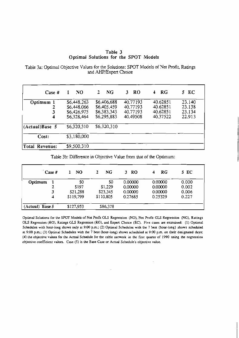
Table 3 Optimal Solutions for the SPOT Models

Table 3a: Optimal Objective Values for the Solutions: SPOT Models of Net Profit, Ratings and AHPExpert Choice

Case # 1 NO 2 NG 3 RO 4 RG 5 EC

Optimum 1 $6,448,263 $6,406,688 40.77 193 40.6285 1 23.140 2 $6,448,066 $6,405,459 40.77193 40.6285 1 23.138 3 $6,426,975 $6,3 83,343 40.77 193 40.6285 1 23.134 4 $6,328,464 $6,295,883 40.49508 40.37522 22.91 3

(Actua1)Base 5 $6,320,3 10 $6,320,3 10

Cost: $3,180,000

Total Revenue: $9,500,3 10

Table 3b: Difference in Objective Value from that of the Optimum:

Case # 1 NO 2 NG 3 RO 4 RG 5 EC

Optimum 1 SO $0 0.00000 0.00000 0.000 2 $197 $1,229 0.00000 0.00000 0.002 3 $2 1,288 523,345 0.00000 0.00000 0.006 4 $1 19.799 $1 10.805 0.27685 0.25329 0.227

(Actual) Base 5 $127,953 $86,378

Optimal Solutions for the SPOT Models of Net Profit OLS Regression (NO). Net Rofit GLS Regression (NG). Ratings OLS Regression (RO). Ratings GLS Regression (RG), and Expen Choice (EC). Five c v e s are examined: (1) Oprimal Schedules with hour-long shows only at 9:00 p.m.; (2) Optimal Schedules with the 7 best (hour-long) shows scheduled at 9:00 p.m.; (3) Optimal Schedules with the 7 best (hour-long) shows scheduled at 9:00 p.m. on their designated days; (4) the objective values for the Actual Schedule for the cable network in the first quarter of 1990 using the regression objecrive coefficient values. C u e (5) is the Base Case or Actual Schedule's objecrive value.

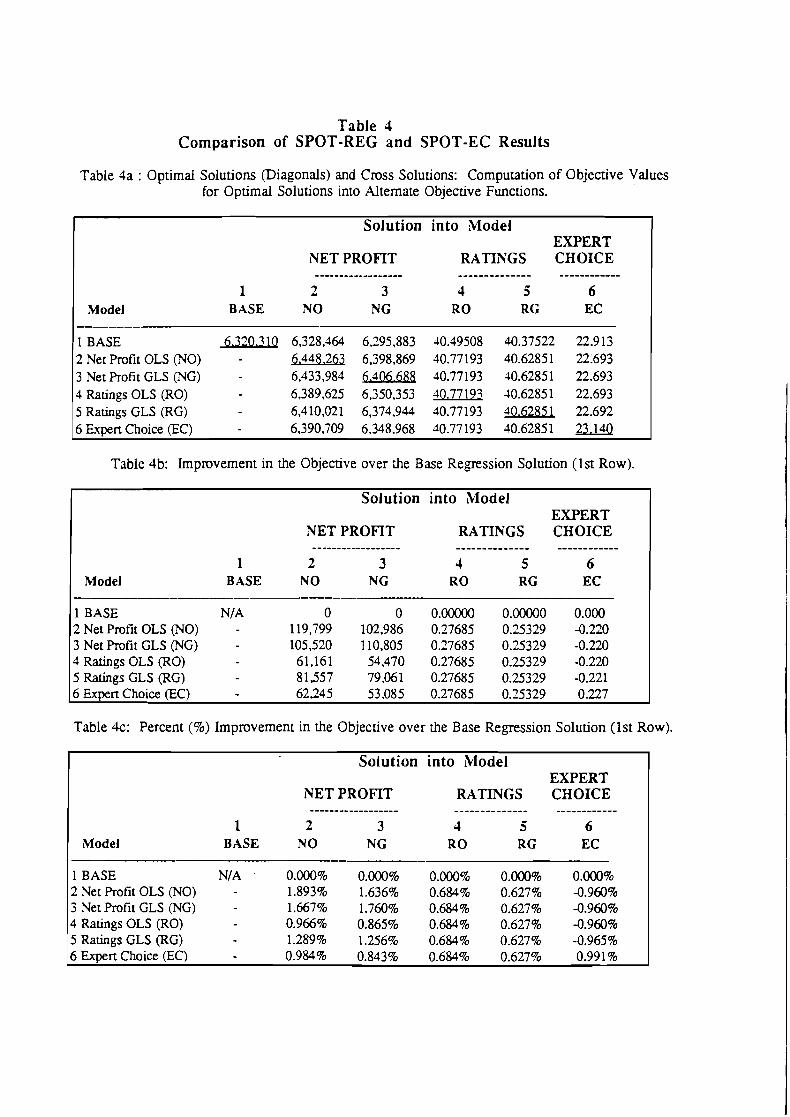
Table 4 Comparison of SPOT-REG and SPOT-EC Results

Table 4a : Optimal Solutions (Diagonals) and Cross Solutions: Computation of Objective Values for Optimal Solutions into Alternate Objective Functions.

Solution into Model EXPERT

NET PROFIT RATINGS CHOICE ------------------ -------------- ------------

1 2 3 4 5 6 Model BASE NO NG RO RG EC

- 1 BASE 6.320.3 1Q 6,328,464 6,295,883 40.49508 40.37522 22.9 13 2 Net Profit OLS (NO) 6.448.263 6,398,869 40.77193 40.62851 22.693 3 Net Profit GLS (NG) 6.433.984 6406.688 40.77193 40.62851 22.693 4 Ratings OLS (RO) 6,389,625 6.350.353 10.77193 40.62851 22.693 5 Ratings GLS (RG) 6,410,021 6,374,944 40.77193 10.6285 1 22.692 6 Expert Choice (EC) 6,390,709 6,348,968 10.77 193 40.6285 1 23.140

Table 4b: Improvement in the Objective over the Base Regression Solution (1st Row).

Solution into Model EXPERT

NET PROFIT RATINGS CHOICE ------------------ -------------- ------------

1 2 3 4 5 6 Model BASE NO NG RO RG EC

-- - 1 BASE N/ A 0 0 0.00000 0.00000 0.000 2 Net Profit OLS (NO) 119,799 102,986 0.27685 0.25329 -0.220 3 Net Profit GLS (NG) 105,520 110,805 0.27685 0.25329 -0.220 4 Ratings OLS (RO) 61,161 54,470 0.27685 0.25329 -0.220 5 Ratings GLS (RG) 81557 79.061 0.27685 0.25329 -0.221 6 Expert Choice (EC) 62245 53,085 0.27685 0.35329 0.227

Table 4c: Percent (9%) Improvement in the Objective over the Base Regression Solution (1st Row).

Solution into model EXPERT

NET PROFIT RATINGS CHOICE ------------------ -------------- ------------

1 2 3 4 5 6 Model BASE NO NG RO RG EC

- ---- 1 BASE N / A 0.000% 0.000% 0.000% 0.000% 0.000% 2 Net Profit OLS (NO) 1.893% 1.636% 0.684% 0.627% -0.960% 3 Net Profit GLS (NG) 1.667% 1.760% 0.684% 0.627% -0.960% 4 Ratings OLS (RO) 0.966% 0.865% 0.684% 0.627% -0.960% 5 Ratings GLS (RG) 1.289% 1.256% 0.684% 0.627% -0.965% 6 Expert Choice (EC) 0.984% 0.843% 0.684% 0.627% 0.991 %

Table 5

Mean Parameter Estimates of the Regression Model

GLS- 2%

OLS- 5%

OLS- 10%

GLS- 10%

MEAN MEAN RMSD* MEAN MEAN RMSD MEAN MEAN RMSD

Perc. Attract. Duration

Mon Tue wed nu Fri Sat

Intercept

R~ Adj. R'

* RMSD = Root Mean Squared Difference of the estimated coefficients, across the 10 replications

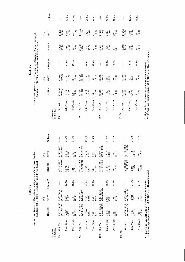
?; ID' - =- -, - -- -, o,z 0 -7- -= - N- - c- YlG a'. " 2 3- r-= 2 5 0 5 7~ ZZ 5: 2 5 =? "m :? =;

7 - 7- -- -- 7 -- -- 7- 2z r z 7- -- -- - d

3 - - -

-- ";; -- -?s 23 2s m s 7 7. -3 &7_ - N Z :o - 7.2

3 - 7 'a- z 52- sg P N- -5; ;; " (?t. - S? 3- 74 ;5 z - 7-: T- z'o 7 7.: ' ;x :% ID- -- 2E 'a- -- Nu 'a- -- Nu 'a- -i N-

'a- &% ' a . VI = <% - - 7.2 'a-

'a- 0 S? *. g :f-? T 2 ID-

- 2 a 0

:

?&? ,s g OD. 7. 'a-

?$ -- $ 2 o;* a m 7 % ID-

- > .- A 0

2

wz g: $3 =. 2 <a - 2s 2: g 8. 7N

'a- z

3 > .- 8

- NOD - - - - - N i

= - a m ?- N -. - : - i= - - - - - V]

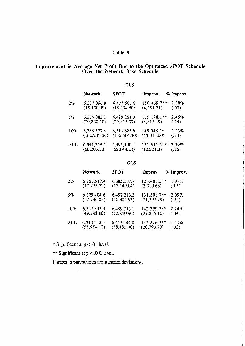
Table 8

Improvement in Average Net Profit Due to the Optimized SPOT Schedule Over the Network Base Schedule

OLS

Network SPOT Improv. % Improv.

ALL 6,341,759.2 6,493,100.4 15 1,341.2** 2.39% (60,203.50) (62.044.20) (10,221.3) (. 16)

GLS

Network SPOT Improv. 9% Improv.

ALL 6,310,218.4 6,442,444.8 132,226.3** 2.10% (56,954.10) (58,185.40) (20.793.70) (.33)

* Significant at p < .O1 level.

** Significant at p < .001 level.

Fi,oures in parentheses are standard deviations.

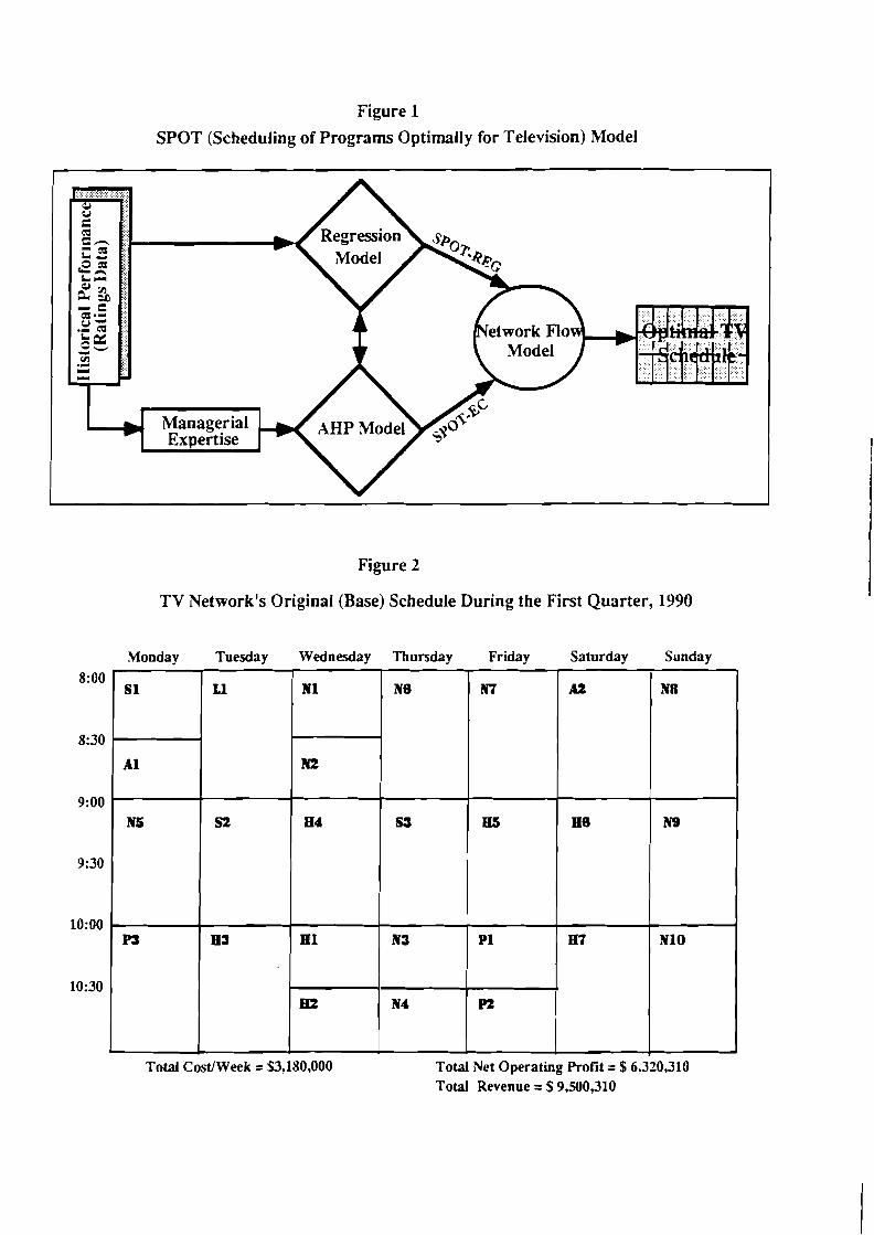
Figure 1

SPOT (Scheduling of Programs Optimally for Television) Model

Figure 2

TV Network's Original (Base) Schedule During the First Quarter, 1990

ep

gz 2 Q

La a4 & $ I E Q .- . -.)

Monday Tuesday Wednesday Thursday Friday Saturday Sunday

i:.

j: ';

; !j iij :..

Z .;

Total Net Operating Profit = $6,320,310 Total Revenue = $9,500,310

. Managerial Expertise

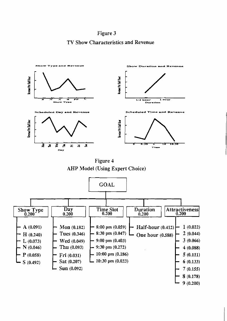
Figure 3

TV Show Characteristics and Revenue

Sho- Typo rnd R e r o m u o Show Duraclon and Revenue

Scheduled Day rnd Revenue Scheduled Time and Revenue

Figure 4 AHP Model (Using Expert Choice)

I

1 I I I Attractiveness

0.200 Show Type

0.200 Day 0.300

Time Slot 0.200

Duration 0.200

- 1 (0.022) - 2 (0.044) - 3 (0.066)

- 4 (0.088) - 5 (0.111)

- 6 (0.133) - 7 (0.155)

- A (0.091)

- H (0.240) - L (0.073) - N (0.046)

- P (0.058)

- S (0.492) - Sun (0.092)

- 8:00 pm (0.059) - lMon (0.182) - Tues (0.346)

- Wed (0.049) - Thu (0.093)

- Fri (0.031) - Sat (0.207)

- Half-hour (0.412) - 8:30 pm (0-047) - one hour ( 0 2 s ) - 9:00 pm (0.403) - 9:30 pm (0.272) - 10:OO pm (0.186) - 10:30 pm (0.033)

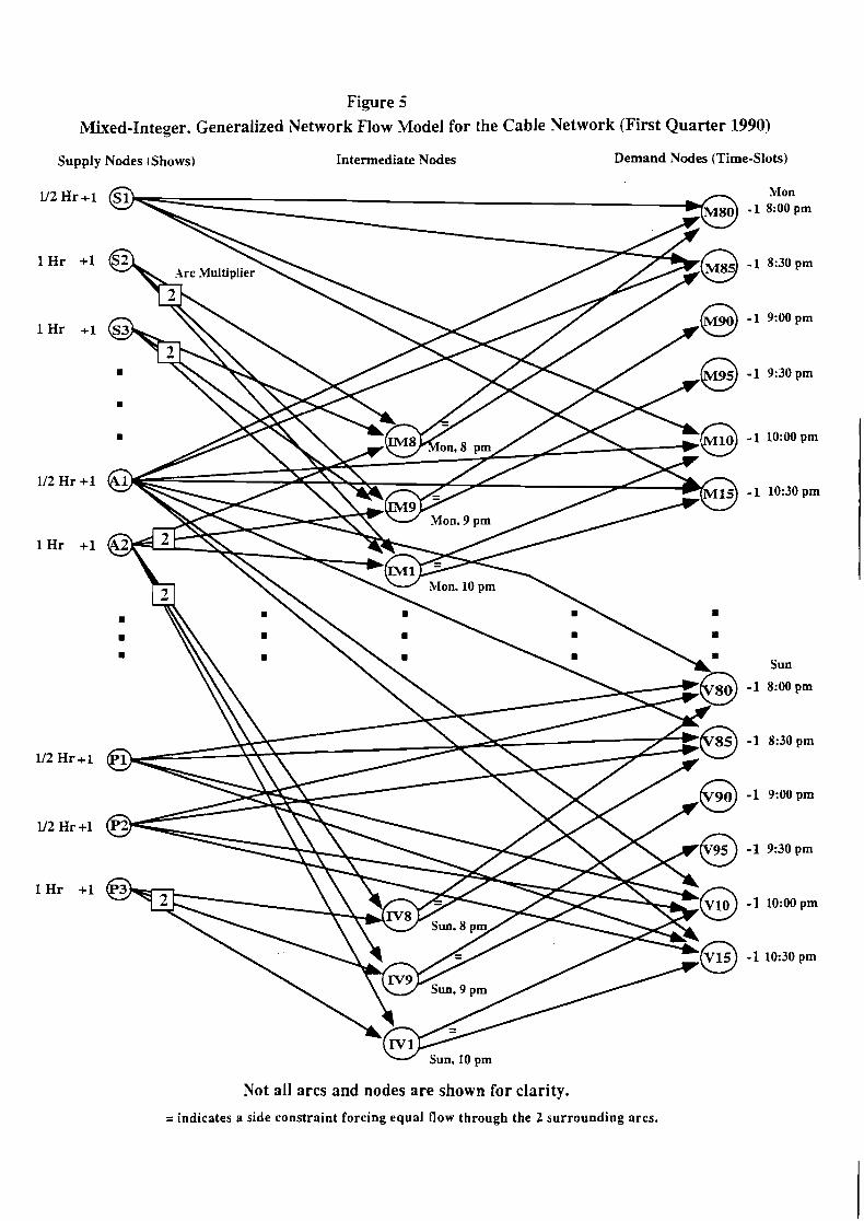
Figure 5

ÿ mixed-Integer. Generalized Network Flow %lode1 for the Cable Network (First Quarter 1990)

Supply Nodes (Shows) Intermediate Nodes Demand Nodes (Time-Slots)

Sun

8:00 prn

Sun, 10 pm

Not all arcs and nodes are shown for clarity. = indicates a side constraint forcing equal flow through the 2 surrounding arcs.

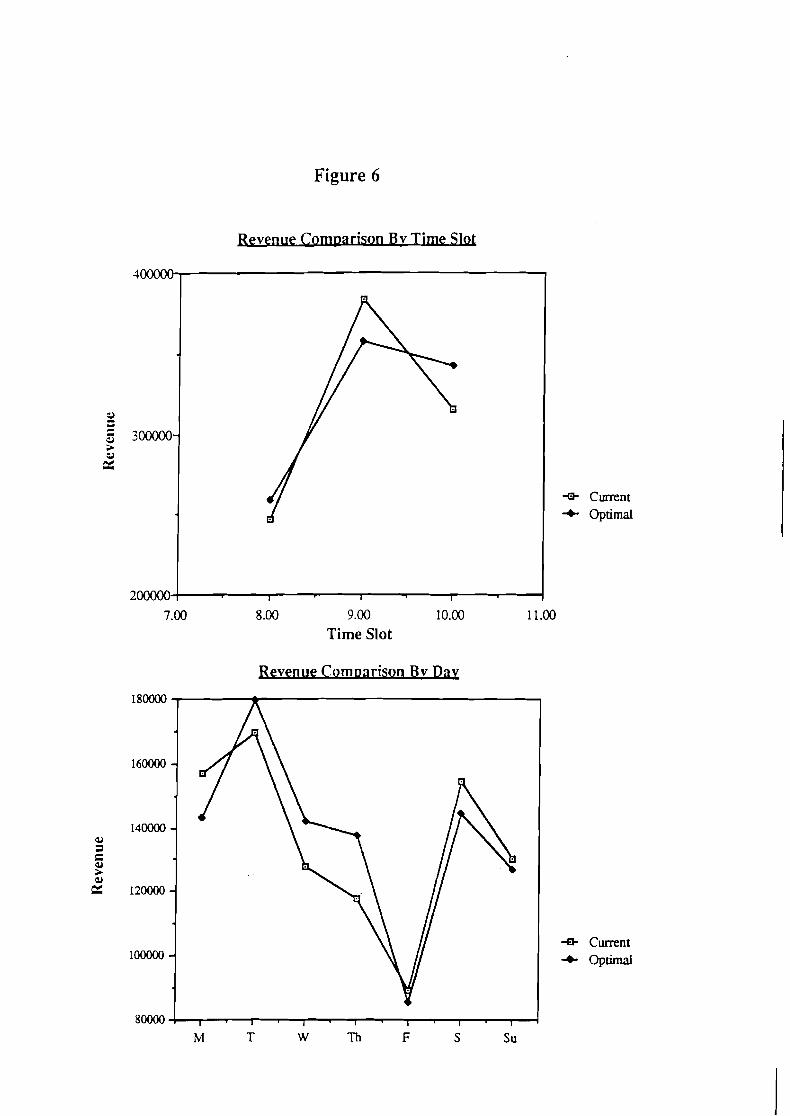
Figure 6

&venue Corngar~son Bv Time Slot

+it- Current + Optimal

7.00 8.00 9.00 10.00 11.00

Time Slot

Bevenue Com~arison Bv Dav

* Current * Optimal

Figure 7

SPOT Optimal Schedule iNet ProlitlOLS) ror First Quarter 1990 (Case 1)

Total CosWeek = $3,180,000

* Indicates a 'best' show at 9:00 pm.

Figure 8

Total Net Operating Profit = S 6 , 4 8 2 6 3 Total Revenue = 5 9,628263

SPOT Optimal Schedule (AHPIExpert Choice) for First Quarter 1990 (Case 1)

Tohl CosWeek = 53.180.000 Objective Value = 23.14 Tohl Net Operating Profit = S 6,390,709 Tohl Revenue = S 9,570,709

Indicates a 'best' show at 9:00 pm.