Seediscussions,stats,andauthorprofilesforthispublicationat:https://www.researchgate.net/publication/31376145

OptimalSensorDeploymentforWirelessSurveillanceSensorNetworksbyaHybridSteady-StateGenetic...

ArticleinIEICETransactionsonCommunications·November2008

DOI:10.1093/ietcom/e91-b.11.3534·Source:OAI

CITATIONS

23

READS

342

5authors,including:

Si-HoCha

ChungwoonUniversity

54PUBLICATIONS194CITATIONS

SEEPROFILE

MinhoJo

KoreaUniversity

91PUBLICATIONS871CITATIONS

SEEPROFILE

AllcontentfollowingthispagewasuploadedbyMinhoJoon17July2017.

Theuserhasrequestedenhancementofthedownloadedfile.

3534IEICE TRANS. COMMUN., VOL.E91–B, NO.11 NOVEMBER 2008

PAPER Special Section on Emerging Technologies for Practical Ubiquitous and Sensor Networks

Optimal Sensor Deployment for Wireless Surveillance SensorNetworks by a Hybrid Steady-State Genetic Algorithm

Jae-Hyun SEO†, Yong-Hyuk KIM†, Hwang-Bin RYOU†, Nonmembers, Si-Ho CHA††,and Minho JO†††a), Members

SUMMARY An important objective of surveillance sensor networks isto effectively monitor the environment, and detect, localize, and classifytargets of interest. The optimal sensor placement enables us to minimizemanpower and time, to acquire accurate information on target situation andmovement, and to rapidly change tactics in the dynamic field. Most ofprevious researches regarding the sensor deployment have been conductedwithout considering practical input factors. Thus in this paper, we applymore real-world input factors such as sensor capabilities, terrain features,target identification, and direction of target movements to the sensor place-ment problem. We propose a novel and efficient hybrid steady-state ge-netic algorithm giving low computational overhead as well as optimal sen-sor placement for enhancing surveillance capability to monitor and locatetarget vehicles. The proposed algorithm introduces new two-dimensionalgeographic crossover and mutation. By using a new simulator adopting theproposed genetic algorithm developed in this paper, we demonstrate suc-cessful applications to the wireless real-world surveillance sensor place-ment problem giving very high detection and classification rates, 97.5%and 87.4%, respectively.key words: wireless sensor networks, surveillance sensor deployment, hy-brid steady-state genetic algorithm

1. Introduction

Wireless sensor networks (WSNs) are utilized to monitorthe areas where traditional networks could not be used.WSNs have been widely implemented in practice suchas disaster intervention, habitat monitoring, microclimateresearch, surveillance, emergency search-and-rescue andmedical care, as sensor capability has improved [1], [2].Currently, surveillance operations require an automated sen-sor deployment system. Especially, an automated sensor al-location and management system [3] is vital to a ground op-eration that monitors the movement of targets. We are muchinterested in the improvement of sensor capability as well asoptimal sensor placement. The optimal sensor emplacementenables us to minimize manpower and time, to acquire accu-rate information on target movement, and to rapidly changetactics in the dynamic field. Therefore, the optimally fittedsensor emplacement allows for us to have a good awarenessof targets.

Manuscript received March 1, 2008.Manuscript revised June 3, 2008.†The authors are with the Department of Computer Science

and Engineering, Kwangwoon University, Korea.††The author is with the Department of Information and Com-

munication Engineering, Sejong University, Korea.†††The author is with Graduate School of Information Manage-

ment and Security, Korea University, Korea.a) E-mail: minhojo@korea.ac.kr

DOI: 10.1093/ietcom/e91–b.11.3534

In general, the position of sensors affects coverage,communication costs, and resource management of surveil-lance sensor networks. Thus we are required to place a sen-sor in the best location. Nevertheless, we randomly deploythe sensors to monitor and locate the target vehicles. Thisrandom deployment may cause sensors to be centralized orto be surrounded by terrain features. It will decrease theprobability of detection and classification of target move-ment. Most of previous literatures regarding the sensor de-ployment have focused their research on theoretical pointswithout considering practical input factors. Thus in this pa-per, we apply more real-world input factors such as sensorcapabilities, terrain features, target identification, and direc-tion of target movements to the wireless surveillance sensorplacement problem.

In addition to the more practical problem-solving con-tribution of this paper, we propose a novel hybrid steady-state genetic algorithm (GA) to solve the practical sensordeployment problem with more complex real-world inputfactors. The optimal sensor placement is a problem of max-imizing coverage and minimizing the number of sensors. Itis a kind of the Minimum Set Cover (MSC) problem. MSCis an NP-hard problem. We here propose a hybrid steady-state GA to find the high-quality solutions of the wirelesssurveillance sensor deployment and apply it to a practicalcase study. The proposed genetic algorithm to solve thereal-world sensor deployment introduces 2-dimensional ge-ographic crossovers and mutations, and local optimizationwhich are unique features. In this paper, the experimentaldata was obtained from a real surveillance situation.

The remainder of this paper is organized as follows:Sect. 2 explains previous studies for the optimal sensor em-placement. Section 3 defines the real-world problem han-dled in this paper. In Sect. 4, we propose a hybrid steady-state genetic algorithm for the optimal sensor deployment.Section 5 describes the environments of experiment and an-alyzes the results of simulation. The paper ends with con-clusions in Sect. 6.

2. Related Work

There have been a number of other studies for the optimalsensor deployment.

Lamm [4], [5] developed sensor employment rules ona system engineering framework using statistical tools suchas Response Surface Methodology (RSM) [6]. Lamm used a

Copyright c© 2008 The Institute of Electronics, Information and Communication Engineers

SEO et al.: OPTIMAL SENSOR DEPLOYMENT FOR WIRELESS SURVEILLANCE SENSOR NETWORKS BY A HYBRID STEADY-STATE GENETIC ALGORITHM3535

computer simulation to test experimental designs. The com-puter simulation uses MapInfo Professional and MapBasicsoftware programs based on the geographic information sys-tem. The major steps of the RSM experiment are as follows.The initial step includes the design for the RSM experimentbefore sensor deployment. The next step is to test whetherthe experiment model is linear or not. The final step is todevelop initial sensor emplacement rules considering trade-off with multi-objectives and to refine them as the steps areiterated. This test requires a lot of time and moreover it isdifficult to conduct elaborate experiments.

Virtual force algorithm (VFA) of Zou et al. [7] em-ployed the repulsive and attractive forces so as to enlargethe coverage for the target region. In VFA, a cluster-headgathers the location information of every sensor. Every sen-sor has a force on it influenced by other sensors, obstacles,and preferential areas. The experiment of VFA shows thatmore sensors should be emplaced around the obstacles thanin the preferential areas. However, the cost of sensor deviceswill be drastically increased because more and more sensorsare needed as the target area is expanded. It will be requiredhow to decrease the number of sensors.

Wang et al. [8] could meet the grid-quorum that a high-density grid sends advertisements along its row and a low-density grid sends requests along its column. They couldachieve better fairness as describing the cascaded move-ment. A direct long movement could be decomposed intomultiple short movements. The accomplished fairness couldmake it possible to relocate sensors evenly. The sensor re-location maximizes coverage and shows higher detectionrates.

Sharp et al. [9] made an experiment on the pursuer-evader problem. The problem is that the evader moves ran-domly in the sensing field and the pursuer tries to capturethe evader by the information from the static wireless sensornetwork. The experiment contributed to building the basicsensor emplacement system significantly.

There were two genetic approaches. Xu et al. [10] pro-posed in 2006 a genetic algorithm to optimize sensor place-ment and to minimize the number of sensors. Zhao et al.showed energy efficient heterogeneous sensor deploymentusing a general genetic algorithm in 2007 [11]. The keyoperators of the algorithms are order-mapped crossover andsimple inversion mutation. And it is difficult to apply themto the real-world because of lack of real-world input factormodeling. They don’t consider the real-world input factorssuch as sensor capabilities, terrain features, target identi-fication, and direction of target movements for the sensorplacement problem which are included in our problem solv-ing. Because our proposed hybrid steady-state genetic algo-rithm uses 2-dimensional geographical crossover and mu-tation while Xu et al. and Zhao et al.’s genetic algorithmsdo not use them, we cannot compare performance results ofboth algorithms and ours.

3. Problem Definition

Sensor capabilities, terrain features, target identification, thedirection of target movements, and more factors are essen-tial to the real-world sensor placement. It is crucial to con-sider how the input factors will affect the target detection.Therefore, we introduce the sensor network elements andperformance evaluation function, and denote input variablesin this section.

3.1 Problem Statement

A seismic sensor can detect vibrations caused by the move-ment of vehicles or human beings. An acoustic sensor candetect acoustic signatures caused by the movement of ve-hicles or human beings. FLIR (Forward-Looking InfraredRadar) is a device that senses infrared radiation. An attri-tion sensor is used to destroy sensors which belong to theother party. A wheeled vehicle is a vehicle that moves onwheels and usually has a container for transporting thingsor people such as trucks. A tracked vehicle is a vehicle thatruns on tracks instead of wheels such as trains.

In our experiment, the targets are classified intowheeled vehicles and tracked vehicles. The terrain featuresconsist of rivers, trees, hills, towns, and open fields. Seis-mic, acoustic, FLIR, and attrition sensors are used for ourexperiment.

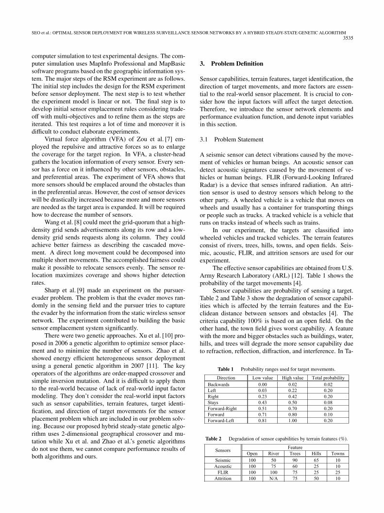
The effective sensor capabilities are obtained from U.S.Army Research Laboratory (ARL) [12]. Table 1 shows theprobability of the target movements [4].

Sensor capabilities are probability of sensing a target.Table 2 and Table 3 show the degradation of sensor capabil-ities which is affected by the terrain features and the Eu-clidean distance between sensors and obstacles [4]. Thecriteria capability 100% is based on an open field. On theother hand, the town field gives worst capability. A featurewith the more and bigger obstacles such as buildings, water,hills, and trees will degrade the more sensor capability dueto refraction, reflection, diffraction, and interference. In Ta-

Table 1 Probability ranges used for target movements.

Table 2 Degradation of sensor capabilities by terrain features (%).

3536IEICE TRANS. COMMUN., VOL.E91–B, NO.11 NOVEMBER 2008

Table 3 Degradation of sensor capabilities by natural logarithmfunction.

Table 4 Notation of input variables and evaluation function.

ble 2, notice that degradation is significant for the featureslike river, trees, hills, and towns.

In Table 3, effective detection rates (Power of Detec-tion, POD) converted by the natural logarithm function, areprovided. C1 and C2 are constant to compute degradation ofsensor capability and D1 (m) and D2 (m) are detection rangeof sensors.

3.2 Input Variables and Evaluation Function

Input variables and evaluation function are defined in Ta-ble 4. Every target moves passing through a grid cell of area5 km × 5 km. The direction of target movements in a gridis defined by a probability given in Table 1 and Formula(2). The frequency of target movements is chosen at ran-dom. Multiple target movements can occur simultaneously

in a grid.We compute the number of undetected targets by the

function. Then, we calculate the detection rate and the cor-rect classification rate as provided in Formula (7). Detectionmeans that sensors sense a target successfully. Classificationaccounts for the case of classifying a type of target success-fully among the detected targets. We consider the dynamicinput variables for our problem, such as target movement di-rection (p) in Tables 1 and 4 and breakdown of sensors de-stroyed (detected) by the attrition sensors of the other partyin Formula (2) and (4).

The following are equations describing the evaluationfunction to test our sensor employment capability. Formula(1) sets the detection rate for each cell based on the dis-tance between the center of each cell and sensors. Formula(2) shows probability ranges used for targets and the coor-dinates of the moved sensor are given by Formula (3). For-mula (4) and Formula (5) present the process of getting thenumbers of detected targets (Cdetect), correctly classified tar-get vehicles (Cclass), and our sensors detected by the attri-tion sensors of the other party (Cattrition), all of which are tobe parameters of simulation.

S (x) =

{POD × R if 0 ≤ x ≤ D1(log (x) ×C1 + C2

) × R if D1 ≤ x ≤ D2(1)

(x, y) =

⎧⎪⎪⎪⎪⎪⎪⎪⎪⎪⎪⎪⎪⎪⎨⎪⎪⎪⎪⎪⎪⎪⎪⎪⎪⎪⎪⎪⎩

(0,−1) if 0 ≤ p ≤ 0.02(−1, 0) if 0.03 ≤ p ≤ 0.22(1, 0) if 0.23 ≤ p ≤ 0.42(0, 0) if 0.43 ≤ p ≤ 0.5(1, 1) if 0.52 ≤ p ≤ 0.7(0, 1) if 0.71 ≤ p ≤ 0.8(−1, 1) if 0.81 ≤ p ≤ 1

(2)

(a, b) = (α, β) + (x, y) (3)

Hl =

{1 if r ∈ R, r < e0 otherwise

Ik =

{1 if r ≤ e,Hl = 10 otherwise

Fi =

{1 if p ∈ R, p < t, Ik = 00 otherwise

G j =

{1 if c ≤ 0.95, Fi = 10 otherwise

(4)

In Formula (4) and Formula (5), i denotes the numberof detected vehicles, j accounts for the number of classifiedvehicles, and l and k stand for the number of our sensors de-tected and destroyed, respectively by the other party. Ik tellswhether or not our sensor is destroyed by the other party’sattrition sensor. Thus Ik will influence the number of de-tecting target vehicles, Fi. If the number of instances of Ik

= 1 increases, the number of detecting target vehicles, Fi

decreases (i.e., the case of Fi = 1 occurs less).

Cdetect =

Wtgt∑i=1

Fi +

Ttgt∑i=1

Fi

SEO et al.: OPTIMAL SENSOR DEPLOYMENT FOR WIRELESS SURVEILLANCE SENSOR NETWORKS BY A HYBRID STEADY-STATE GENETIC ALGORITHM3537

Cclass =

Wtgt∑j=1

G j +

Ttgt∑j=1

G j (5)

Cattrition =

Wtgt∑k=1

Ik +

Ttgt∑k=1

Ik

U =(Wtgt + Ttgt

)−Cdetect (6)

D = 1 − U(Wtgt + Ttgt

) ,C = Cclass

Cdetect(7)

When the target vehicles move passing through thearea, we compute the number of undetected targets by ap-plying Formulas (2), (3), (4), and (5). Finally, we computethe detection rate and the correct classification rate by For-mula (7). Notice that Cattrition is not for equations but onlyfor monitoring the number of our sensors destroyed by theother party. The number of our sensors destroyed by attri-tion sensors is already reflected in Formula (4).

4. The Proposed Genetic Algorithm

In this section, our hybrid steady-state genetic algorithm isproposed, and the principal operators to optimize sensor em-placement are illustrated.

4.1 Hybrid Steady-State GA

Genetic algorithms (GAs) were first proposed by Holland[13]. GAs are a class of probabilistic optimization algo-rithms and inspired by the biological evolution process.GAs model the concept of natural selection and genetic in-heritance.

Our hybrid steady-state GA is the mixture of thesteady-state GA and the hybrid GA. The generational GAsreplace the whole or a part of solutions with new offspringper each generation. Meanwhile, the steady-state GA re-places just one solution with a new offspring per each gen-eration. We classify GAs into hybrid or pure ones accordingto whether or not local optimization is applied. The hybridGA uses local optimization for improvement of offspringproduced by crossover.

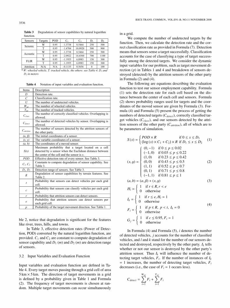
Figure 1 shows the flow diagram of our hybrid steady-state GA. The steps of the proposed GA are described in thefollowing.

1. Step 1 generates population based on a random deploy-ment.

2. Step 2 is the selection of Parent 1 and Parent 2.3. Step 3 is the process of the crossover which creates an

offspring by the genes’ recombination of Parent 1 andParent 2.

4. Step 4 is the process of the mutation that varies eachgene of the offspring by some probability. Then wemake simulation for evaluating the offspring and getthe information of detection rate and classification one.

5. Step 5 is the process of the local optimization. The op-erator moves each sensor to the best adjacent position

Fig. 1 A flow diagram of the proposed hybrid steady-state GA.

by trying to move the sensor to the eight neighbor cells.6. Step 6 is the process of the replacement that replaces

with the final offspring a solution of the population.7. All steps will be iterated until the stop condition is sat-

isfied. The stop condition is set up to the number ofgenerations.

4.2 Crossovers and Mutations

We apply two different crossover operations and two mu-tation operations in the proposed hybrid steady-state GA.The two crossover operations are block crossover and tablemarriage crossover and the two mutation operations includeswap mutation and attractive/repulsive (AR) mutation.

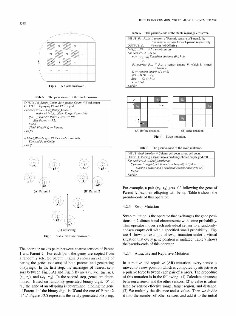
4.2.1 Block Crossover

Anderson et al. [14] suggested a block uniform crossover ona two-dimensional matrix chromosome that tessellated thechromosome into i× j blocks; the gene in the block is copiedfrom a uniformly selected parent. In this paper, we do notuse a random property because in our preliminary test it didseldom give any effects on the performance. Figure 2 showsthe block crossover, a modified version of the original blockuniform crossover. Table 5 shows the pseudo-code of thismodified operator.

4.2.2 Stable Marriage Crossover

A stable marriage problem [15] has two finite sets: the setof men and that of women. It is designed for finding stablematching which is just a one-to-one mapping between bothsexes. In this paper, we apply the stable marriage problem toa new crossover operator named stable marriage crossover.

3538IEICE TRANS. COMMUN., VOL.E91–B, NO.11 NOVEMBER 2008

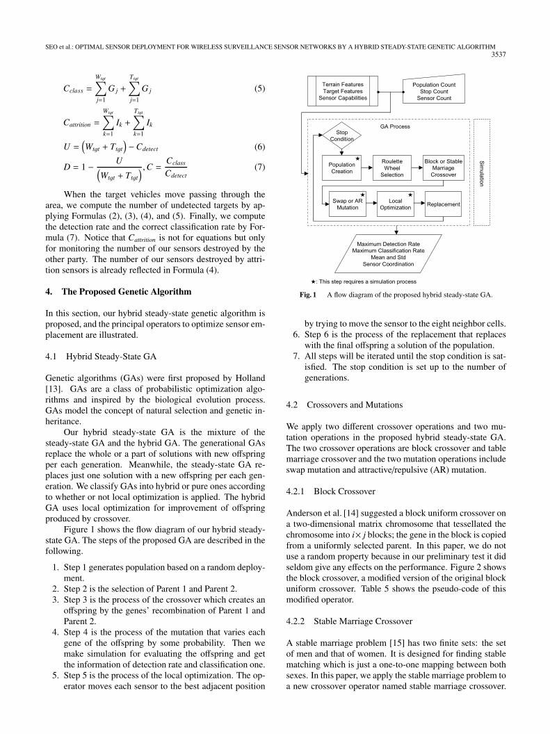
Fig. 2 A block crossover.

Table 5 The pseudo-code of the block crossover.

Fig. 3 Stable marriage crossover.

The operator makes pairs between nearest sensors of Parent1 and Parent 2. For each pair, the genes are copied froma randomly selected parent. Figure 3 shows an example ofparing the genes (sensors) of both parents and generatingoffsprings. In the first step, the marriages of nearest sen-sors between Fig. 3(A) and Fig. 3(B) are (x1, x2), (y1, y2),(z1, z2), and (w1, w2). In the second step, genes are deter-mined. Based on randomly generated binary digit, ‘0’ or‘1,’ the gene of an offspring is determined: cloning the geneof Parent 1 if the binary digit is ‘0’and the one of Parent 2if ‘1.’ Figure 3(C) represents the newly generated offspring.

Table 6 The pseudo-code of the stable marriage crossover.

Fig. 4 Swap mutation.

Table 7 The pseudo-code of the swap mutation.

For example, a pair (x1, x2) gets ‘0,’ following the gene ofParent 1, i.e., their offspring will be x1. Table 6 shows thepseudo-code of this operator.

4.2.3 Swap Mutation

Swap mutation is the operator that exchanges the gene posi-tions on 2-dimensional chromosome with some probability.This operator moves each individual sensor to a randomly-chosen empty cell with a specified small probability. Fig-ure 4 shows an example of swap mutation under a virtualsituation that every gene position is mutated. Table 7 showsthe pseudo-code of this operator.

4.2.4 Attractive and Repulsive Mutation

In attractive and repulsive (AR) mutation, every sensor ismoved to a new position which is computed by attractive orrepulsive force between each pair of sensors. The procedureof this mutation is in the following. (1) Calculate distancesbetween a sensor and the other sensors. (2) α value is calcu-lated by sensor effective range, target region, and distance.(3) We multiply the distance and α value. Then we divideit into the number of other sensors and add it to the initial

SEO et al.: OPTIMAL SENSOR DEPLOYMENT FOR WIRELESS SURVEILLANCE SENSOR NETWORKS BY A HYBRID STEADY-STATE GENETIC ALGORITHM3539

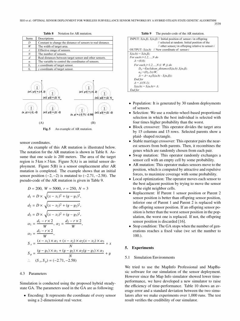
Table 8 Notation for AR mutation.

Fig. 5 An example of AR mutation.

sensor coordinates.An example of this AR mutation is illustrated below.

The notation for the AR mutation is shown in Table 8. As-sume that one scale is 200 meters. The area of the targetregion is 5 km × 5 km. Figure 5(A) is an initial sensor de-ployment. Figure 5(B) is a sensor emplacement after ARmutation is completed. The example shows that an initialsensor position (−2,−2) is mutated to (−2.71,−2.58). Thepseudo-code of the AR mutation is given in Table 9.

D = 200, W = 5000, r = 250, N = 3

d1 = D ×√

(x − x1)2 + (y − y1)2,

d2 = D ×√

(x − x2)2 + (y − y2)2,

d3 = D ×√

(x − x3)2 + (y − y3)2,

α1 =d1 − r × 2

W, α2 =

d2 − r × 2W

,

α3 =d3 − r × 2

W,

S x =(x − x1) × α1 + (x − x2) × α2(x − x3) × α3

N+ x

S y =(y − y1) × α1 + (y − y2) × α2(y − y3) × α3

N+ y

∴ (S x, S y) = (−2.71,−2.58)

4.3 Parameters

Simulation is conducted using the proposed hybrid steady-state GA. The parameters used in the GA are as following:

• Encoding: It represents the coordinate of every sensorusing a 2-dimensional real vector.

Table 9 The pseudo-code of the AR mutation.

• Population: It is generated by 30 random deploymentsof sensors.• Selection: We use a roulette-wheel-based proportional

selection in which the best individual is selected withfour times higher probability than the worst.• Block crossover: This operator divides the target area

by 15 columns and 15 rows. Selected parents show aplaid- shaped rectangle.• Stable marriage crossover: This operator pairs the near-

est sensors from both parents. Then, it recombines thegenes which are randomly chosen from each pair.• Swap mutation: This operator randomly exchanges a

sensor cell with an empty cell by some probability.• AR mutation: This operator makes sensors move to the

position, which is computed by attractive and repulsiveforces, to maximize coverage with some probability.• Local optimization: The operator moves each sensor to

the best adjacent position by trying to move the sensorto the eight neighbor cells.• Replacement: If Parent 1 sensor position or Parent 2

sensor position is better than offspring sensor position,inferior one of Parent 1 and Parent 2 is replaced withthe offspring sensor position. If an offspring sensor po-sition is better than the worst sensor position in the pop-ulation, the worst one is replaced. If not, the offspringsensor position is discarded [16].• Stop condition: The GA stops when the number of gen-

erations reaches a fixed value (we set the number to100.).

5. Experiments

5.1 Simulation Environments

We tried to use the MapInfo Professional and MapBa-sic software for our simulation of the sensor deployment.However since the Map Info simulator showed lower time-performance, we have developed a new simulator to raisethe efficiency of time-performance. Table 10 shows an av-erage error and a standard deviation between the two simu-lators after we make experiments over 1,000 runs. The testresult verifies the credibility of our simulator.

3540IEICE TRANS. COMMUN., VOL.E91–B, NO.11 NOVEMBER 2008

Table 10 Comparison of an average error between MapInfo simulatorand our simulator.

Table 11 Simulation environment.

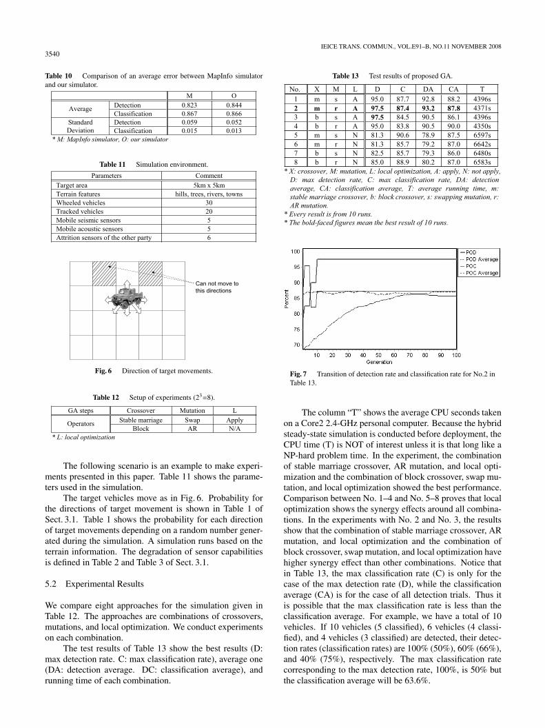
Fig. 6 Direction of target movements.

Table 12 Setup of experiments (23=8).

The following scenario is an example to make experi-ments presented in this paper. Table 11 shows the parame-ters used in the simulation.

The target vehicles move as in Fig. 6. Probability forthe directions of target movement is shown in Table 1 ofSect. 3.1. Table 1 shows the probability for each directionof target movements depending on a random number gener-ated during the simulation. A simulation runs based on theterrain information. The degradation of sensor capabilitiesis defined in Table 2 and Table 3 of Sect. 3.1.

5.2 Experimental Results

We compare eight approaches for the simulation given inTable 12. The approaches are combinations of crossovers,mutations, and local optimization. We conduct experimentson each combination.

The test results of Table 13 show the best results (D:max detection rate. C: max classification rate), average one(DA: detection average. DC: classification average), andrunning time of each combination.

Table 13 Test results of proposed GA.

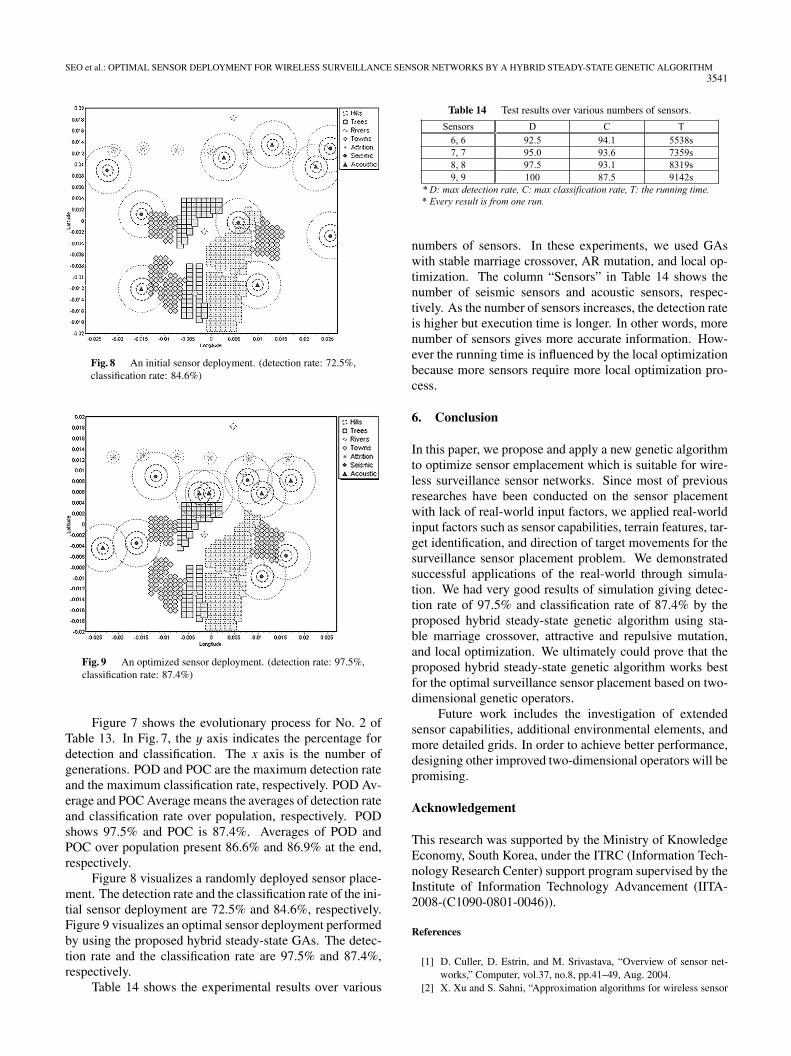
Fig. 7 Transition of detection rate and classification rate for No.2 inTable 13.

The column “T” shows the average CPU seconds takenon a Core2 2.4-GHz personal computer. Because the hybridsteady-state simulation is conducted before deployment, theCPU time (T) is NOT of interest unless it is that long like aNP-hard problem time. In the experiment, the combinationof stable marriage crossover, AR mutation, and local opti-mization and the combination of block crossover, swap mu-tation, and local optimization showed the best performance.Comparison between No. 1–4 and No. 5–8 proves that localoptimization shows the synergy effects around all combina-tions. In the experiments with No. 2 and No. 3, the resultsshow that the combination of stable marriage crossover, ARmutation, and local optimization and the combination ofblock crossover, swap mutation, and local optimization havehigher synergy effect than other combinations. Notice thatin Table 13, the max classification rate (C) is only for thecase of the max detection rate (D), while the classificationaverage (CA) is for the case of all detection trials. Thus itis possible that the max classification rate is less than theclassification average. For example, we have a total of 10vehicles. If 10 vehicles (5 classified), 6 vehicles (4 classi-fied), and 4 vehicles (3 classified) are detected, their detec-tion rates (classification rates) are 100% (50%), 60% (66%),and 40% (75%), respectively. The max classification ratecorresponding to the max detection rate, 100%, is 50% butthe classification average will be 63.6%.

SEO et al.: OPTIMAL SENSOR DEPLOYMENT FOR WIRELESS SURVEILLANCE SENSOR NETWORKS BY A HYBRID STEADY-STATE GENETIC ALGORITHM3541

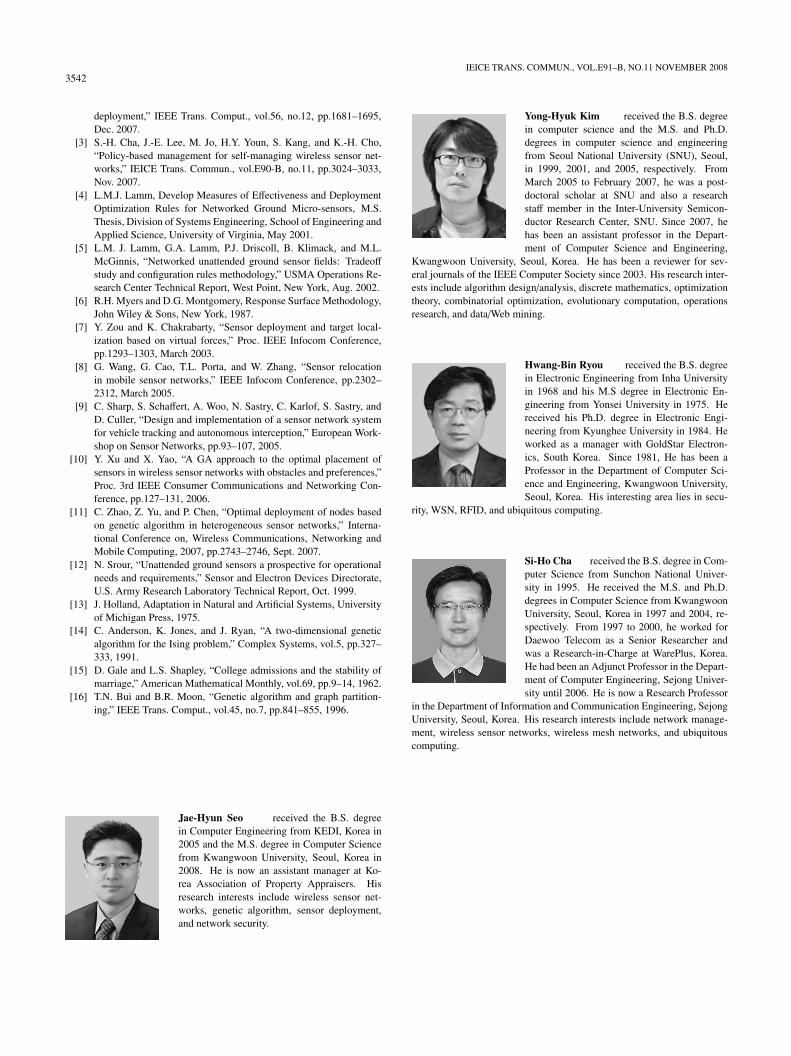
Fig. 8 An initial sensor deployment. (detection rate: 72.5%,classification rate: 84.6%)

Fig. 9 An optimized sensor deployment. (detection rate: 97.5%,classification rate: 87.4%)

Figure 7 shows the evolutionary process for No. 2 ofTable 13. In Fig. 7, the y axis indicates the percentage fordetection and classification. The x axis is the number ofgenerations. POD and POC are the maximum detection rateand the maximum classification rate, respectively. POD Av-erage and POC Average means the averages of detection rateand classification rate over population, respectively. PODshows 97.5% and POC is 87.4%. Averages of POD andPOC over population present 86.6% and 86.9% at the end,respectively.

Figure 8 visualizes a randomly deployed sensor place-ment. The detection rate and the classification rate of the ini-tial sensor deployment are 72.5% and 84.6%, respectively.Figure 9 visualizes an optimal sensor deployment performedby using the proposed hybrid steady-state GAs. The detec-tion rate and the classification rate are 97.5% and 87.4%,respectively.

Table 14 shows the experimental results over various

Table 14 Test results over various numbers of sensors.

numbers of sensors. In these experiments, we used GAswith stable marriage crossover, AR mutation, and local op-timization. The column “Sensors” in Table 14 shows thenumber of seismic sensors and acoustic sensors, respec-tively. As the number of sensors increases, the detection rateis higher but execution time is longer. In other words, morenumber of sensors gives more accurate information. How-ever the running time is influenced by the local optimizationbecause more sensors require more local optimization pro-cess.

6. Conclusion

In this paper, we propose and apply a new genetic algorithmto optimize sensor emplacement which is suitable for wire-less surveillance sensor networks. Since most of previousresearches have been conducted on the sensor placementwith lack of real-world input factors, we applied real-worldinput factors such as sensor capabilities, terrain features, tar-get identification, and direction of target movements for thesurveillance sensor placement problem. We demonstratedsuccessful applications of the real-world through simula-tion. We had very good results of simulation giving detec-tion rate of 97.5% and classification rate of 87.4% by theproposed hybrid steady-state genetic algorithm using sta-ble marriage crossover, attractive and repulsive mutation,and local optimization. We ultimately could prove that theproposed hybrid steady-state genetic algorithm works bestfor the optimal surveillance sensor placement based on two-dimensional genetic operators.

Future work includes the investigation of extendedsensor capabilities, additional environmental elements, andmore detailed grids. In order to achieve better performance,designing other improved two-dimensional operators will bepromising.

Acknowledgement

This research was supported by the Ministry of KnowledgeEconomy, South Korea, under the ITRC (Information Tech-nology Research Center) support program supervised by theInstitute of Information Technology Advancement (IITA-2008-(C1090-0801-0046)).

References

[1] D. Culler, D. Estrin, and M. Srivastava, “Overview of sensor net-works,” Computer, vol.37, no.8, pp.41–49, Aug. 2004.

[2] X. Xu and S. Sahni, “Approximation algorithms for wireless sensor

3542IEICE TRANS. COMMUN., VOL.E91–B, NO.11 NOVEMBER 2008

deployment,” IEEE Trans. Comput., vol.56, no.12, pp.1681–1695,Dec. 2007.

[3] S.-H. Cha, J.-E. Lee, M. Jo, H.Y. Youn, S. Kang, and K.-H. Cho,“Policy-based management for self-managing wireless sensor net-works,” IEICE Trans. Commun., vol.E90-B, no.11, pp.3024–3033,Nov. 2007.

[4] L.M.J. Lamm, Develop Measures of Effectiveness and DeploymentOptimization Rules for Networked Ground Micro-sensors, M.S.Thesis, Division of Systems Engineering, School of Engineering andApplied Science, University of Virginia, May 2001.

[5] L.M. J. Lamm, G.A. Lamm, P.J. Driscoll, B. Klimack, and M.L.McGinnis, “Networked unattended ground sensor fields: Tradeoffstudy and configuration rules methodology,” USMA Operations Re-search Center Technical Report, West Point, New York, Aug. 2002.

[6] R.H. Myers and D.G. Montgomery, Response Surface Methodology,John Wiley & Sons, New York, 1987.

[7] Y. Zou and K. Chakrabarty, “Sensor deployment and target local-ization based on virtual forces,” Proc. IEEE Infocom Conference,pp.1293–1303, March 2003.

[8] G. Wang, G. Cao, T.L. Porta, and W. Zhang, “Sensor relocationin mobile sensor networks,” IEEE Infocom Conference, pp.2302–2312, March 2005.

[9] C. Sharp, S. Schaffert, A. Woo, N. Sastry, C. Karlof, S. Sastry, andD. Culler, “Design and implementation of a sensor network systemfor vehicle tracking and autonomous interception,” European Work-shop on Sensor Networks, pp.93–107, 2005.

[10] Y. Xu and X. Yao, “A GA approach to the optimal placement ofsensors in wireless sensor networks with obstacles and preferences,”Proc. 3rd IEEE Consumer Communications and Networking Con-ference, pp.127–131, 2006.

[11] C. Zhao, Z. Yu, and P. Chen, “Optimal deployment of nodes basedon genetic algorithm in heterogeneous sensor networks,” Interna-tional Conference on, Wireless Communications, Networking andMobile Computing, 2007, pp.2743–2746, Sept. 2007.

[12] N. Srour, “Unattended ground sensors a prospective for operationalneeds and requirements,” Sensor and Electron Devices Directorate,U.S. Army Research Laboratory Technical Report, Oct. 1999.

[13] J. Holland, Adaptation in Natural and Artificial Systems, Universityof Michigan Press, 1975.

[14] C. Anderson, K. Jones, and J. Ryan, “A two-dimensional geneticalgorithm for the Ising problem,” Complex Systems, vol.5, pp.327–333, 1991.

[15] D. Gale and L.S. Shapley, “College admissions and the stability ofmarriage,” American Mathematical Monthly, vol.69, pp.9–14, 1962.

[16] T.N. Bui and B.R. Moon, “Genetic algorithm and graph partition-ing,” IEEE Trans. Comput., vol.45, no.7, pp.841–855, 1996.

Jae-Hyun Seo received the B.S. degreein Computer Engineering from KEDI, Korea in2005 and the M.S. degree in Computer Sciencefrom Kwangwoon University, Seoul, Korea in2008. He is now an assistant manager at Ko-rea Association of Property Appraisers. Hisresearch interests include wireless sensor net-works, genetic algorithm, sensor deployment,and network security.

Yong-Hyuk Kim received the B.S. degreein computer science and the M.S. and Ph.D.degrees in computer science and engineeringfrom Seoul National University (SNU), Seoul,in 1999, 2001, and 2005, respectively. FromMarch 2005 to February 2007, he was a post-doctoral scholar at SNU and also a researchstaff member in the Inter-University Semicon-ductor Research Center, SNU. Since 2007, hehas been an assistant professor in the Depart-ment of Computer Science and Engineering,

Kwangwoon University, Seoul, Korea. He has been a reviewer for sev-eral journals of the IEEE Computer Society since 2003. His research inter-ests include algorithm design/analysis, discrete mathematics, optimizationtheory, combinatorial optimization, evolutionary computation, operationsresearch, and data/Web mining.

Hwang-Bin Ryou received the B.S. degreein Electronic Engineering from Inha Universityin 1968 and his M.S degree in Electronic En-gineering from Yonsei University in 1975. Hereceived his Ph.D. degree in Electronic Engi-neering from Kyunghee University in 1984. Heworked as a manager with GoldStar Electron-ics, South Korea. Since 1981, He has been aProfessor in the Department of Computer Sci-ence and Engineering, Kwangwoon University,Seoul, Korea. His interesting area lies in secu-

rity, WSN, RFID, and ubiquitous computing.

Si-Ho Cha received the B.S. degree in Com-puter Science from Sunchon National Univer-sity in 1995. He received the M.S. and Ph.D.degrees in Computer Science from KwangwoonUniversity, Seoul, Korea in 1997 and 2004, re-spectively. From 1997 to 2000, he worked forDaewoo Telecom as a Senior Researcher andwas a Research-in-Charge at WarePlus, Korea.He had been an Adjunct Professor in the Depart-ment of Computer Engineering, Sejong Univer-sity until 2006. He is now a Research Professor

in the Department of Information and Communication Engineering, SejongUniversity, Seoul, Korea. His research interests include network manage-ment, wireless sensor networks, wireless mesh networks, and ubiquitouscomputing.

SEO et al.: OPTIMAL SENSOR DEPLOYMENT FOR WIRELESS SURVEILLANCE SENSOR NETWORKS BY A HYBRID STEADY-STATE GENETIC ALGORITHM3543

Minho Jo received B.S. degree in IndustrialEngineering, Chosun Univ., South Korea and hisPh.D. in Department of Industrial and SystemsEngineering, Lehigh University, Bethlehem, PA,USA in 1994. He worked as a staff researcherwith Samsung Electronics, South Korea and wasprofessor of School of Ubiquitous Computingand Systems, Sejong Cyber University, Seoul,South Korea. He is now a Research Professorof Graduate School of Information Managementand Security, Korea Univ., Seoul, South Korea.

Prof. Jo is Executive Director of Korean Society for Internet Information(KSII) and Board of Trustees of Institute of Electronics Engineers of Ko-rea (IEEK). He is Editor-in-Chief and Chair of the Steering Committee ofKSII Transactions on Internet and Information Systems, General Chair ofInternational Ubiquitous Conference, and Co-chair of International Con-ference on Ubiquitous Convergence Technology. Dr. Jo is Editor of Jour-nal of Wireless Communications and Mobile Computing, and AssociateEditor of Journal of Security and Communication Networks published byWiley and Sons, respectively. He is Associate Editor of Journal of Com-puter Systems, Networks, and Communications published by Hindawi. Heserves as Chairman of IEEE/ACM WiMax/WiBro Services and QoS Man-agement Symposium, IWCMC 2008. He is Technical Program Committeeof IEEE ICC 2008, 2009 and IEEE GLOBECOM 2008, 2009, respectively.His interesting area lies in wireless ad-hoc sensor networks and wirelessmesh networks, RFID, security in communication networks, machine in-telligence in communications, and pervasive computing/networking.

View publication statsView publication stats