Option Valuation

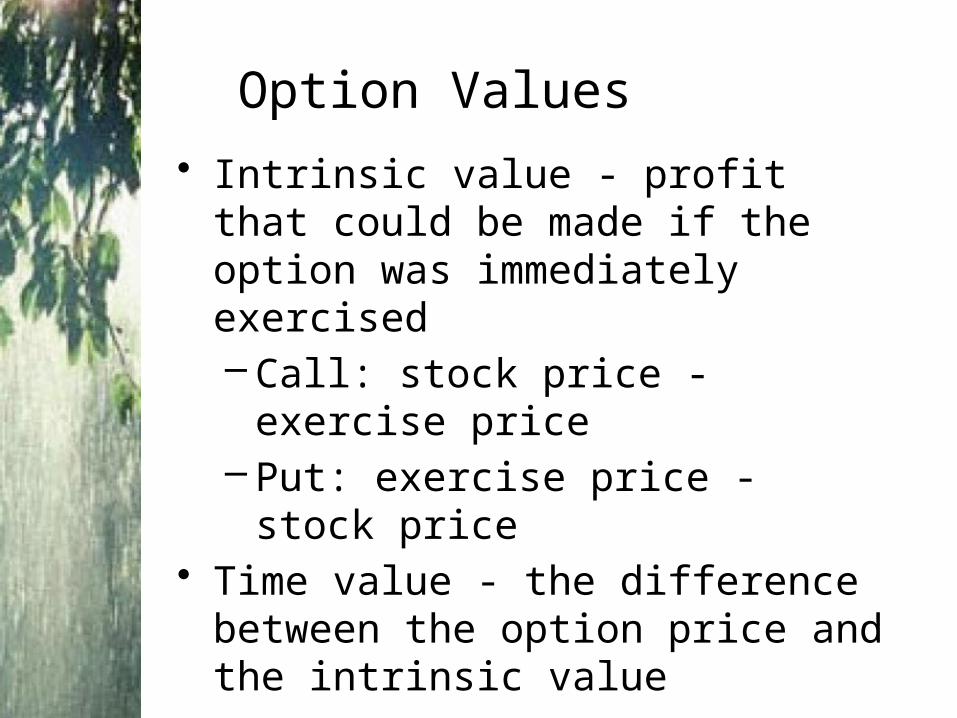
• Intrinsic value - profit that could be made if the option was immediately exercised– Call: stock price - exercise price– Put: exercise price - stock price

• Time value - the difference between the option price and the intrinsic value

Option Values

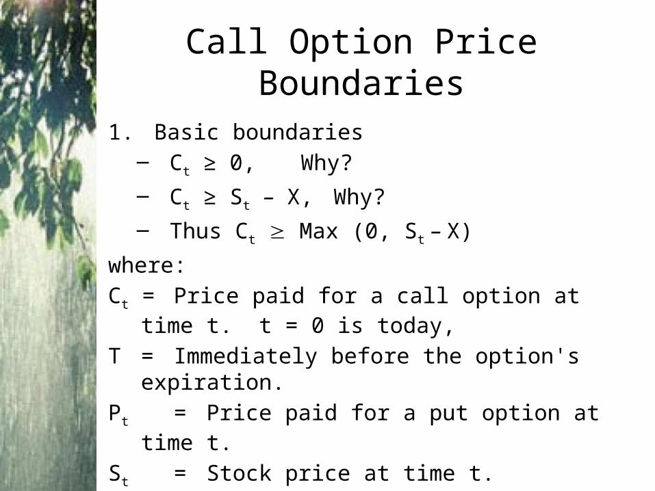
Call Option Price Boundaries

1. Basic boundaries – Ct ≥ 0, Why?

– Ct ≥ St – X, Why?

– Thus Ct Max (0, St – X)

where:

Ct = Price paid for a call option at time t. t = 0 is today,

T = Immediately before the option's expiration.

Pt = Price paid for a put option at time t.

St = Stock price at time t.

X = Exercise or Strike Price (X or E)

Call Option Price Boundaries

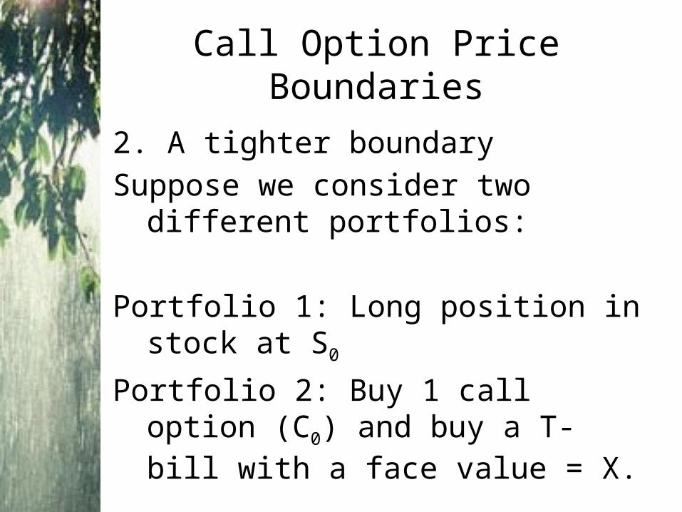
2. A tighter boundary

Suppose we consider two different portfolios:

Portfolio 1: Long position in stock at S0

Portfolio 2: Buy 1 call option (C0) and buy a T-bill with a face value = X.

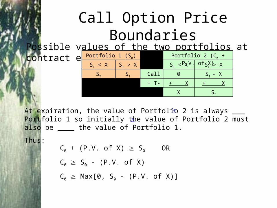
Call Option Price BoundariesPossible values of the two portfolios at contract expiration:

STX

+ X+ X+ T-Bill

ST - X0CallSTST

ST > XST < XST > XST < X

Portfolio 2 (C0 + P.V. of X)Portfolio 1 (S0)

At expiration, the value of Portfolio 2 is always ___ Portfolio 1 so initially the value of Portfolio 2 must also be ____ the value of Portfolio 1.

Thus:

C0 + (P.V. of X) S0 OR

C0 S0 - (P.V. of X)

C0 Max[0, S0 - (P.V. of X)]

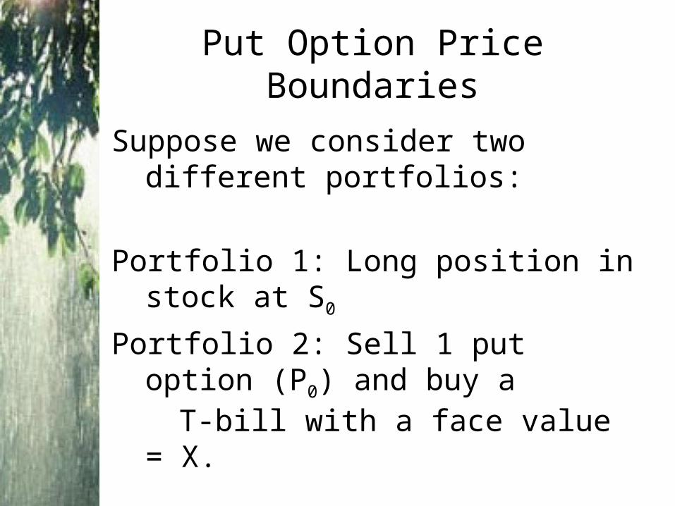
Put Option Price Boundaries

Suppose we consider two different portfolios:

Portfolio 1: Long position in stock at S0

Portfolio 2: Sell 1 put option (P0) and buy a

T-bill with a face value = X.

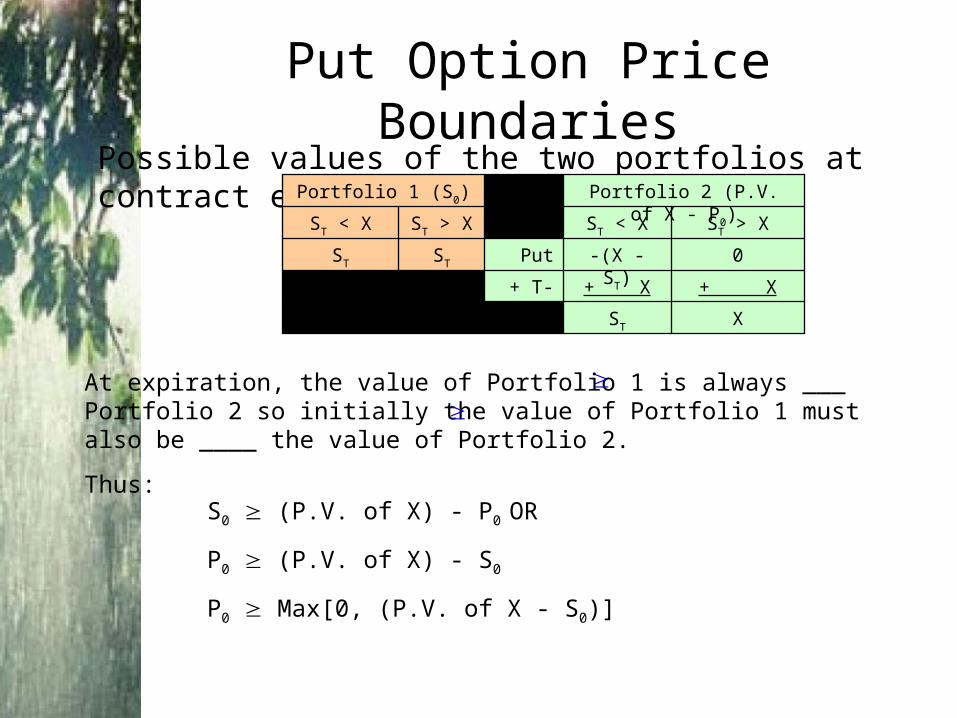
Put Option Price BoundariesPossible values of the two portfolios at contract expiration:

XST

+ X+ X+ T-Bill

0-(X - ST)PutSTST

ST > XST < XST > XST < X

Portfolio 2 (P.V. of X - P0)Portfolio 1 (S0)

At expiration, the value of Portfolio 1 is always ___ Portfolio 2 so initially the value of Portfolio 1 must also be ____ the value of Portfolio 2.

Thus:

S0 (P.V. of X) - P0 OR

P0 (P.V. of X) - S0

P0 Max[0, (P.V. of X - S0)]

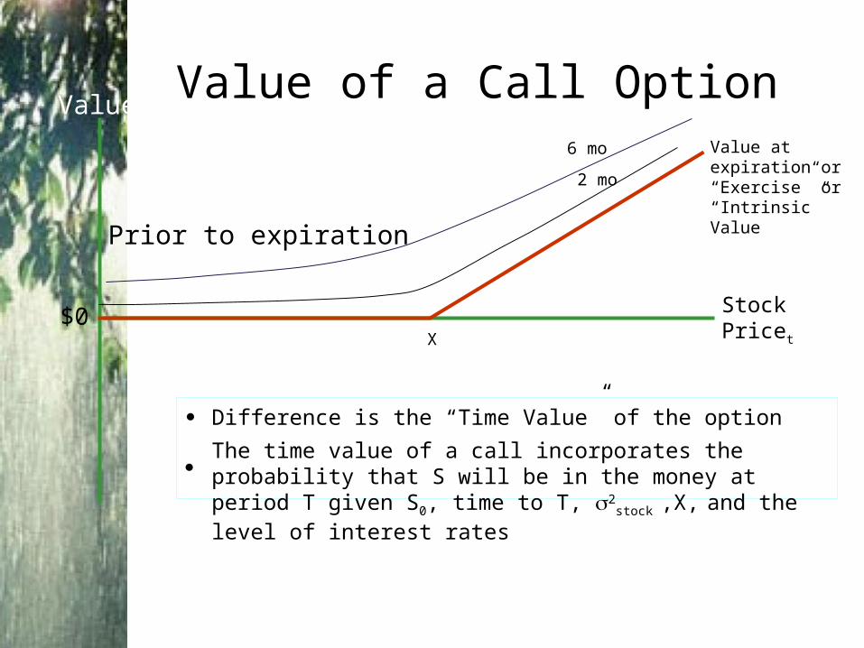
Value of a Call Option

X

Stock Pricet

Value

$0

Prior to expiration

Value at expiration or “Exercise” or “Intrinsic” Value

6 mo

2 mo

Difference is the “Time Value” of the option

The time value of a call incorporates the probability that S will be in the money at period T given S0, time to T, 2

stock ,X, and the level of interest rates

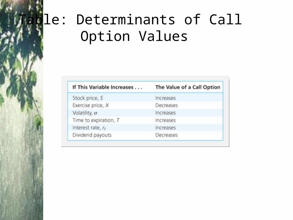
Table: Determinants of Call Option Values

Restrictions on Option Value: Call

• Call value cannot be negative. The option payoff is zero at worst, and highly positive at best.

• Call value cannot exceed the stock value.

• Lower bound = adjusted intrinsic value:C > S0 - PV (X) - PV (D)

(D=dividend)

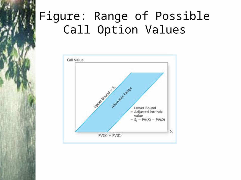
Figure: Range of Possible Call Option Values

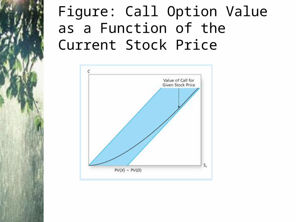
Figure: Call Option Value as a Function of the Current Stock Price

Early Exercise: Calls• The right to exercise an American

call early is valueless as long as the stock pays no dividends until the option expires.

• The value of American and European calls is therefore identical.

• The call gains value as the stock price rises. Since the price can rise infinitely, the call is “worth more alive than dead.”

Early Exercise: Puts

• American puts are worth more than European puts, all else equal.

• The possibility of early exercise has value because:– The value of the stock cannot fall below

zero.– Once the firm is bankrupt, it is optimal

to exercise the American put immediately because of the time value of money.

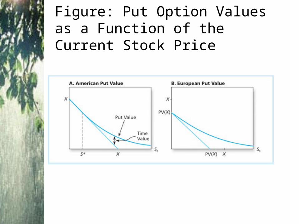
Figure: Put Option Values as a Function of the Current Stock Price

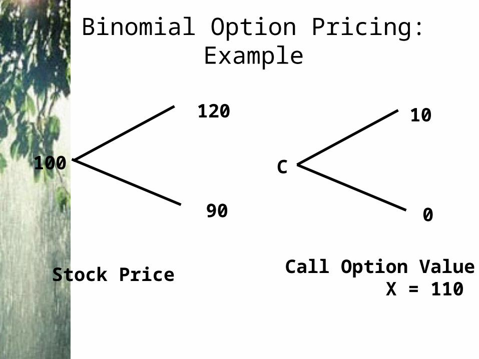
100

120

90

Stock Price

C

10

0

Call Option Value X = 110

Binomial Option Pricing: Example

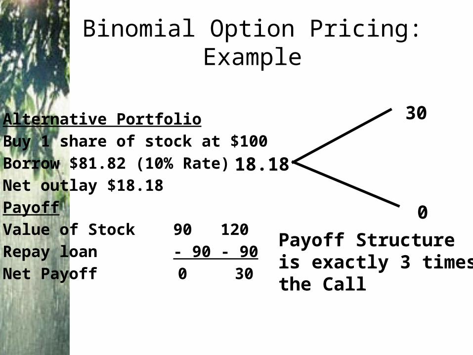
Alternative Portfolio

Buy 1 share of stock at $100

Borrow $81.82 (10% Rate)

Net outlay $18.18

Payoff

Value of Stock 90 120

Repay loan - 90 - 90

Net Payoff 0 30

18.18

30

0

Payoff Structureis exactly 3 timesthe Call

Binomial Option Pricing: Example

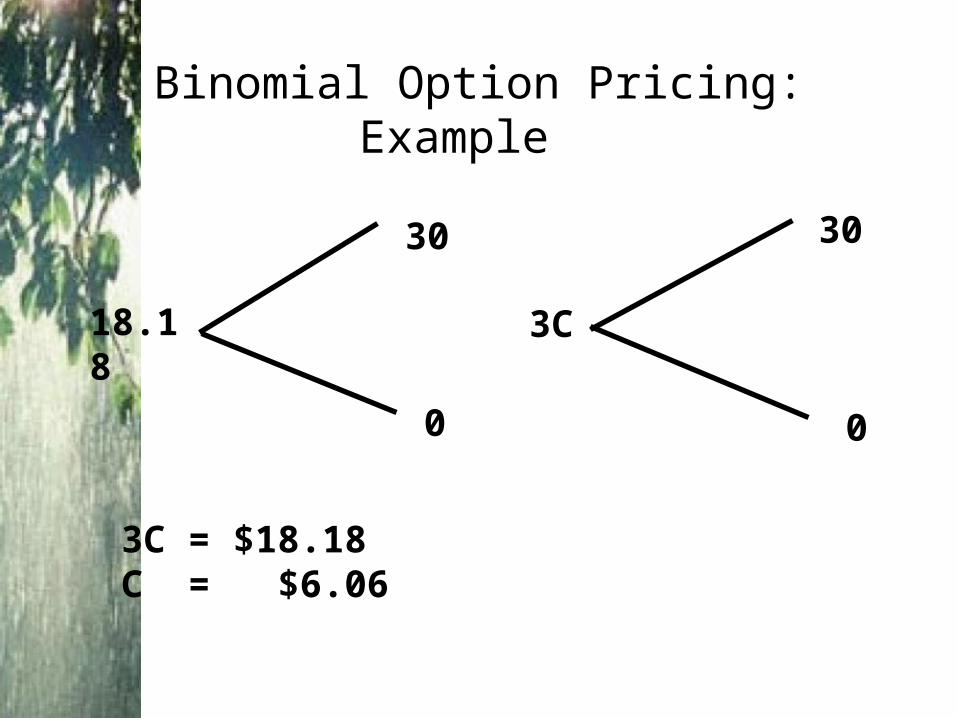
18.18

30

0

3C

30

0

3C = $18.18C = $6.06

Binomial Option Pricing: Example

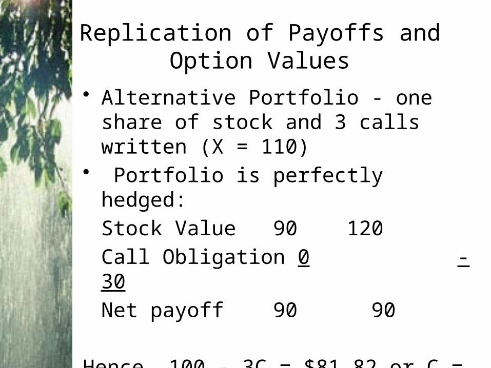
• Alternative Portfolio - one share of stock and 3 calls written (X = 110)

• Portfolio is perfectly hedged:

Stock Value 90 120

Call Obligation 0 -30

Net payoff 90 90

Hence 100 - 3C = $81.82 or C = $6.06

Replication of Payoffs and Option Values

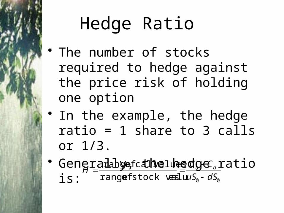
Hedge Ratio

• The number of stocks required to hedge against the price risk of holding one option

• In the example, the hedge ratio = 1 share to 3 calls or 1/3.

• Generally, the hedge ratio is:

00esstock valu of range

valuescall of range

dSuS

CCH du

• Assume that we can break the year into three intervals.

• For each interval the stock could increase by 20% or decrease by 10%.

• Assume the stock is initially selling at $100.

Expanding to Consider Three Intervals

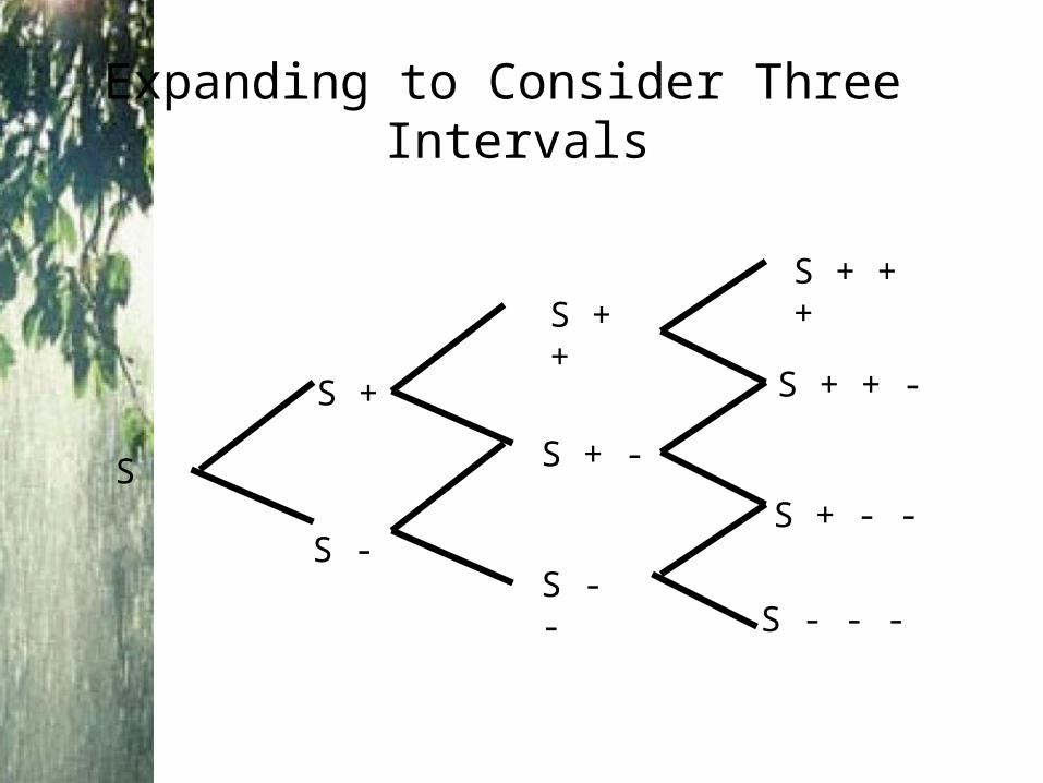
S

S +

S + +

S -S - -

S + -

S + + +

S + + -

S + - -

S - - -

Expanding to Consider Three Intervals

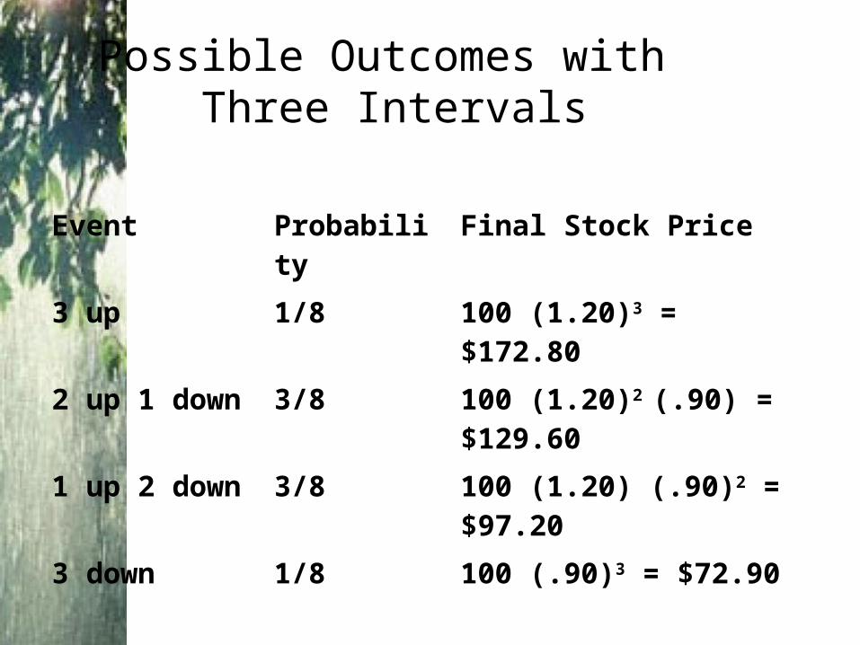
Possible Outcomes with Three Intervals

Event Probability Final Stock Price

3 up 1/8 100 (1.20)3 = $172.80

2 up 1 down 3/8 100 (1.20)2 (.90) = $129.60

1 up 2 down 3/8 100 (1.20) (.90)2 = $97.20

3 down 1/8 100 (.90)3 = $72.90

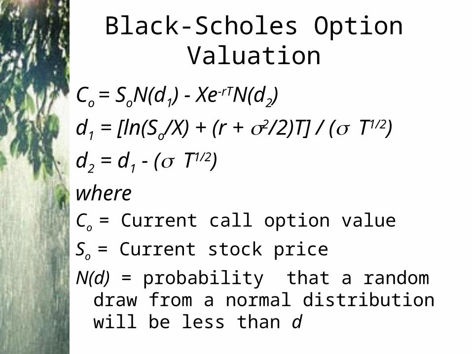
Co = SoN(d1) - Xe-rTN(d2)

d1 = [ln(So/X) + (r + 2/2)T] / (T1/2)

d2 = d1 - (T1/2)

whereCo = Current call option value

So = Current stock price

N(d) = probability that a random draw from a normal distribution will be less than d

Black-Scholes Option Valuation

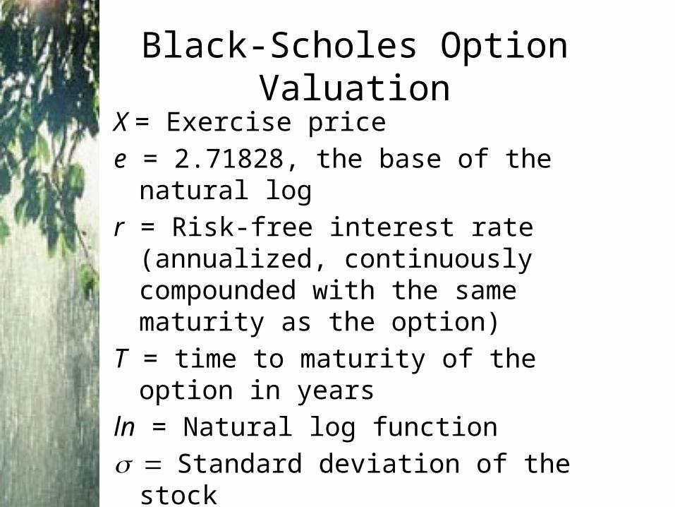
X = Exercise price

e = 2.71828, the base of the natural log

r = Risk-free interest rate (annualized, continuously compounded with the same maturity as the option)

T = time to maturity of the option in years

ln = Natural log function

Standard deviation of the stock

Black-Scholes Option Valuation

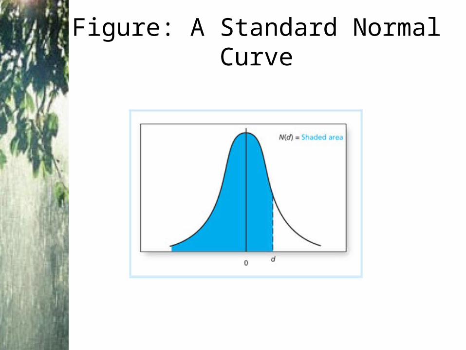
Figure: A Standard Normal Curve

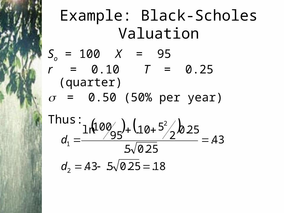
So = 100 X = 95r = 0.10 T = 0.25 (quarter)= 0.50 (50% per year)

Thus:

Example: Black-Scholes Valuation

18.25.05.43.

43.25.05.

25.02510.95

100ln

2

2

1

d

d

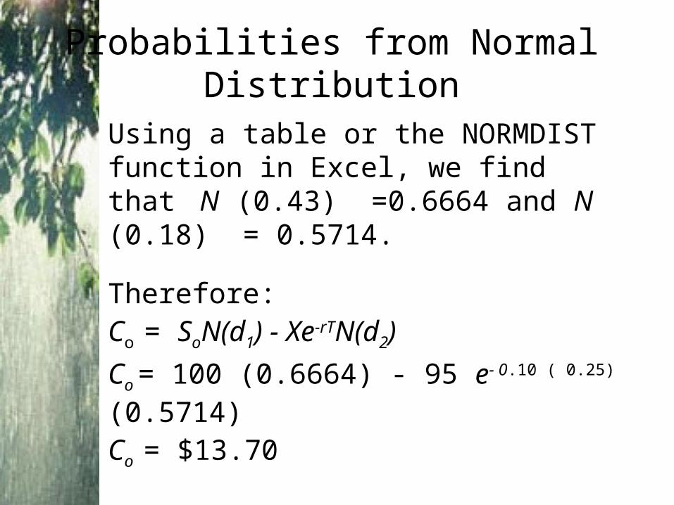
Using a table or the NORMDIST function in Excel, we find that N (0.43) =0.6664 and N (0.18) = 0.5714.

Therefore:Co = SoN(d1) - Xe-rTN(d2)

Co = 100 (0.6664) - 95 e- 0.10 ( 0.25) (0.5714)

Co = $13.70

Probabilities from Normal Distribution

Implied Volatility• Implied volatility is volatility for the

stock implied by the option price.• Using Black-Scholes and the actual

price of the option, solve for volatility.• Is the implied volatility consistent with

the stock?

Call Option Value

Black-Scholes Model with Dividends

• The Black Scholes call option formula applies to stocks that do not pay dividends.

• What if dividends ARE paid?• One approach is to replace the stock

price with a dividend adjusted stock price

Replace S0 with S0 - PV (Dividends)

Example: Black-Scholes Put Valuation

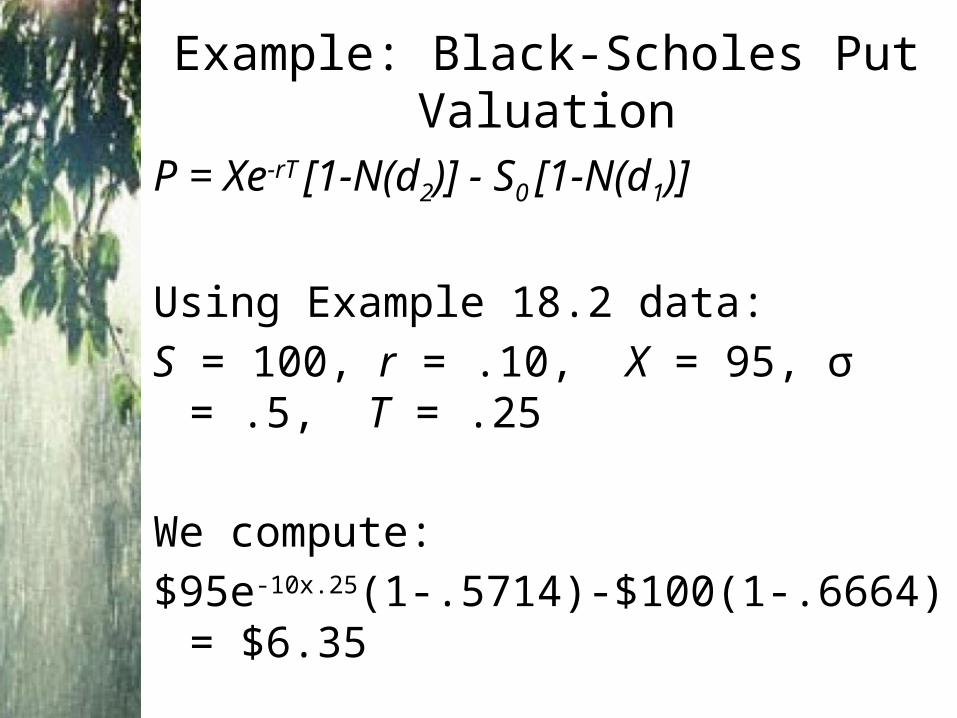
P = Xe-rT [1-N(d2)] - S0 [1-N(d1)]

Using Example 18.2 data:

S = 100, r = .10, X = 95, σ = .5, T = .25

We compute:

$95e-10x.25(1-.5714)-$100(1-.6664) = $6.35

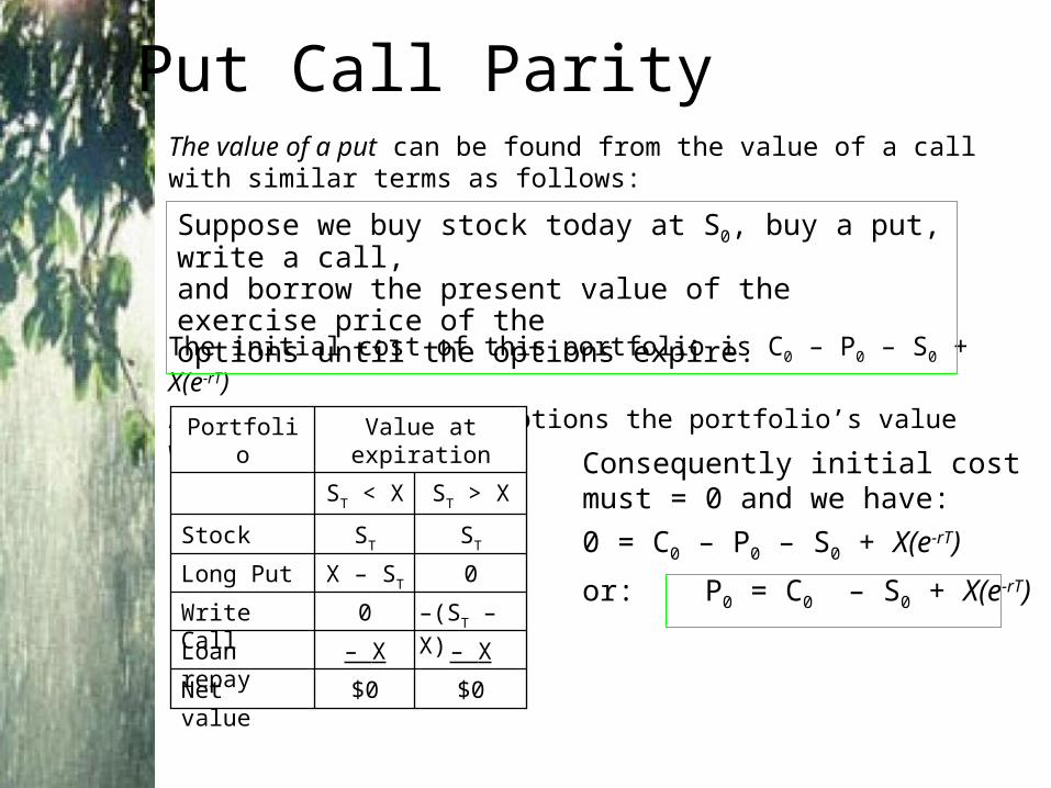
Put Call ParityThe value of a put can be found from the value of a call with similar terms as follows:

The initial cost of this portfolio is C0 – P0 – S0 + X(e-rT)

At expiration of the options the portfolio’s value will be

$0$0Net value

– X– XLoan repay

–(ST – X)0Write Call

0X – STLong Put

STSTStock

ST > XST < X

Value at expirationPortfolio Consequently initial cost must = 0

and we have:

0 = C0 – P0 – S0 + X(e-rT)

or: P0 = C0 – S0 + X(e-rT)

Suppose we buy stock today at S0, buy a put, write a call, and borrow the present value of the exercise price of the options until the options expire.

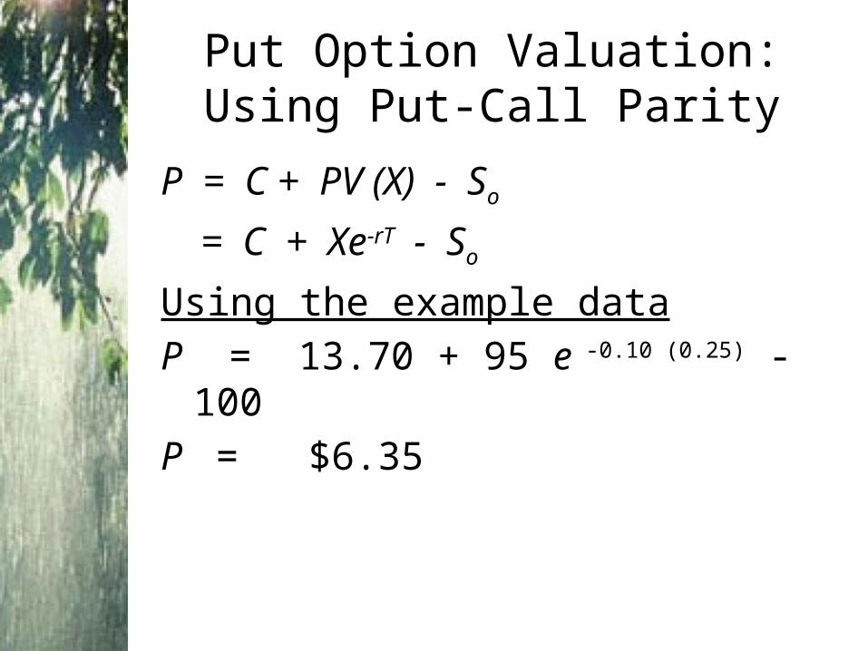
P = C + PV (X) - So

= C + Xe-rT - So

Using the example data

P = 13.70 + 95 e -0.10 (0.25) - 100

P = $6.35

Put Option Valuation: Using Put-Call Parity

Empirical Evidence on Option Pricing

• The Black-Scholes formula performs worst for options on stocks with high dividend payouts.

• The implied volatility of all options on a given stock with the same expiration date should be equal.– Empirical test show that implied

volatility actually falls as exercise price increases.

– This may be due to fears of a market crash.

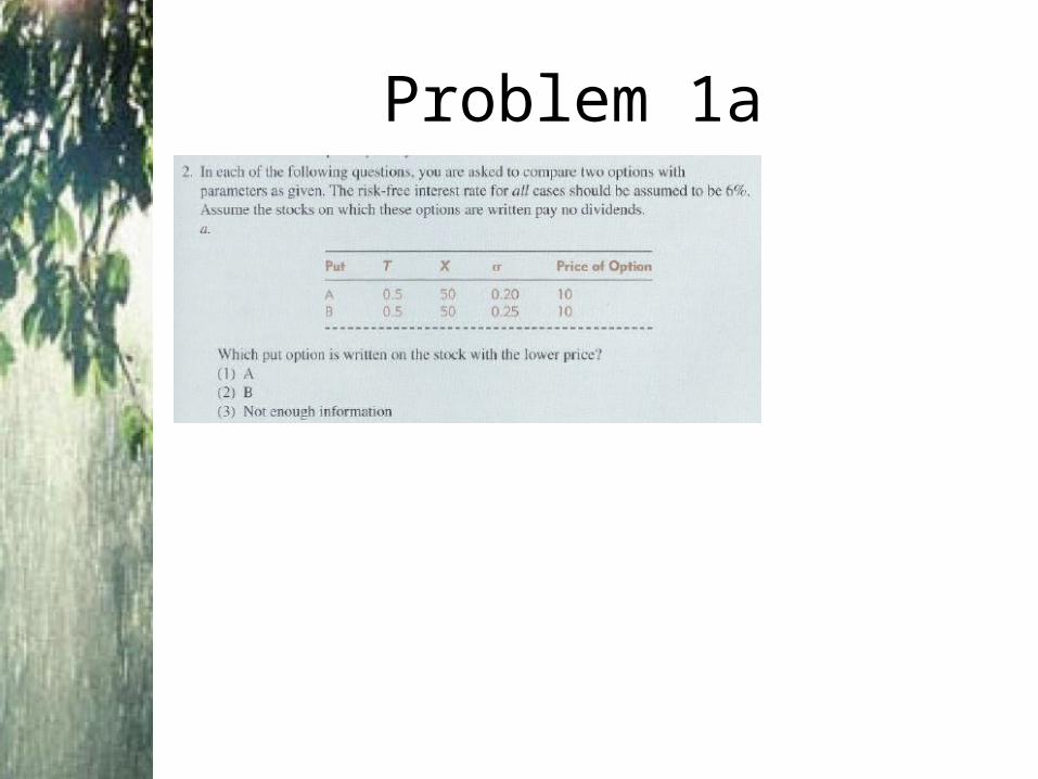
Problem 1a

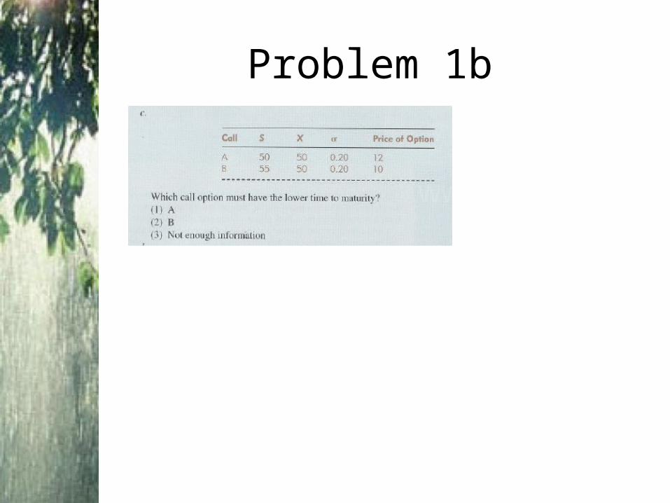
Problem 1b

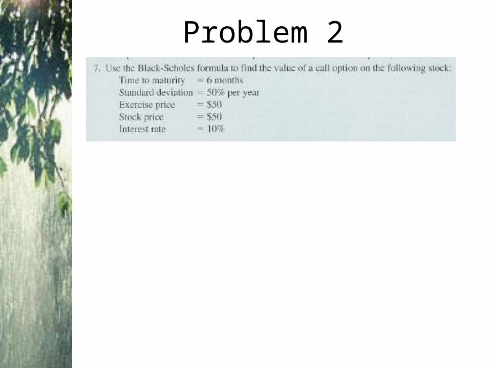
Problem 2

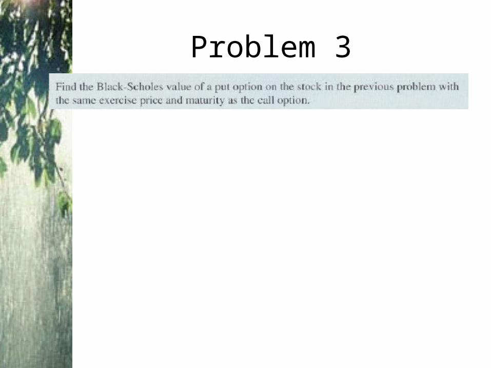
Problem 3