ORF 245 Fundamentals of StatisticsChapter 7

Confidence Intervals

Robert Vanderbei

Fall 2015

Slides last edited on December 10, 2015

http://www.princeton.edu/∼rvdb

Election Polling

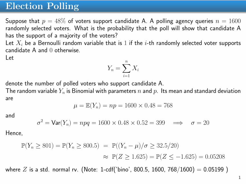
Suppose that p = 48% of voters support candidate A. A polling agency queries n = 1600randomly selected voters. What is the probability that the poll will show that candidate Ahas the support of a majority of the voters?Let Xi be a Bernoulli random variable that is 1 if the i-th randomly selected voter supportscandidate A and 0 otherwise.Let

Yn =n∑

i=1

Xi

denote the number of polled voters who support candidate A.The random variable Yn is Binomial with parameters n and p. Its mean and standard deviationare

µ = E(Yn) = np = 1600× 0.48 = 768

andσ2 = Var(Yn) = npq = 1600× 0.48× 0.52 = 399 =⇒ σ = 20

Hence,

P(Yn ≥ 801) = P(Yn ≥ 800.5) = P((Yn − µ)/σ ≥ 32.5/20)

≈ P(Z ≥ 1.625) = P(Z ≤ −1.625) = 0.05208

where Z is a std. normal rv. (Note: 1-cdf(’bino’, 800.5, 1600, 768/1600) = 0.05199 )1

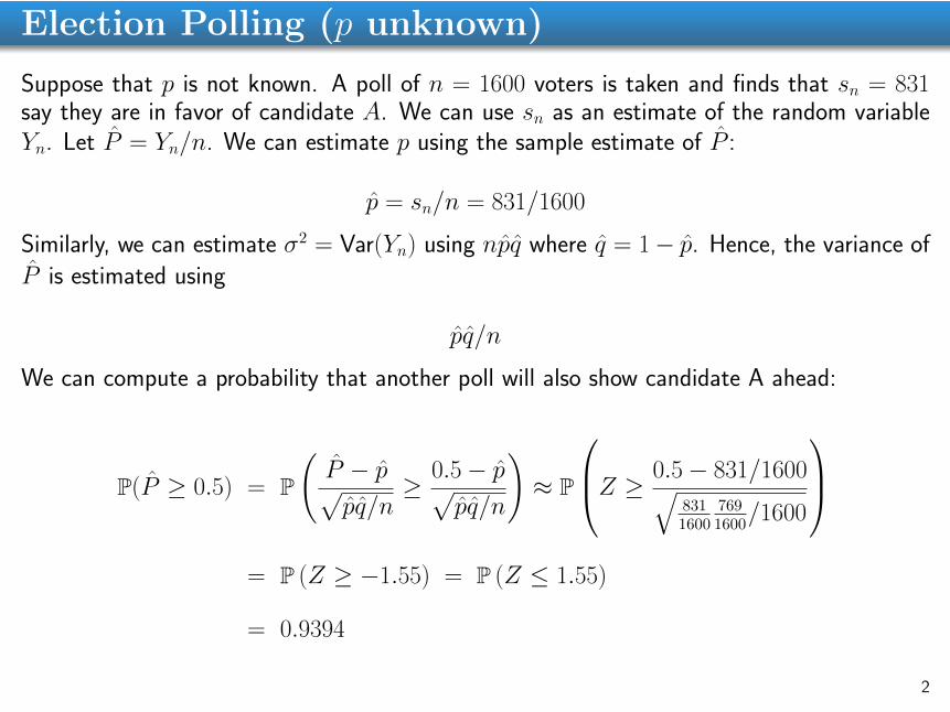
Election Polling (p unknown)

Suppose that p is not known. A poll of n = 1600 voters is taken and finds that sn = 831say they are in favor of candidate A. We can use sn as an estimate of the random variableYn. Let P̂ = Yn/n. We can estimate p using the sample estimate of P̂ :

p̂ = sn/n = 831/1600

Similarly, we can estimate σ2 = Var(Yn) using np̂q̂ where q̂ = 1− p̂. Hence, the variance ofP̂ is estimated using

p̂q̂/n

We can compute a probability that another poll will also show candidate A ahead:

P(P̂ ≥ 0.5) = P

(P̂ − p̂√p̂q̂/n

≥ 0.5− p̂√p̂q̂/n

)≈ P

Z ≥ 0.5− 831/1600√8311600

7691600

/1600

= P (Z ≥ −1.55) = P (Z ≤ 1.55)

= 0.9394

2

Election Polling – Confidence Interval

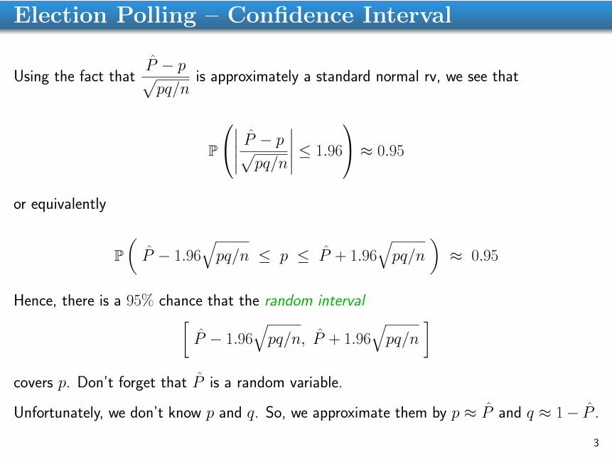
Using the fact thatP̂ − p√pq/n

is approximately a standard normal rv, we see that

P

∣∣∣∣∣ P̂ − p√pq/n

∣∣∣∣∣ ≤ 1.96

≈ 0.95

or equivalently

P(P̂ − 1.96

√pq/n ≤ p ≤ P̂ + 1.96

√pq/n

)≈ 0.95

Hence, there is a 95% chance that the random interval[P̂ − 1.96

√pq/n, P̂ + 1.96

√pq/n

]covers p. Don’t forget that P̂ is a random variable.

Unfortunately, we don’t know p and q. So, we approximate them by p ≈ P̂ and q ≈ 1− P̂ .

3

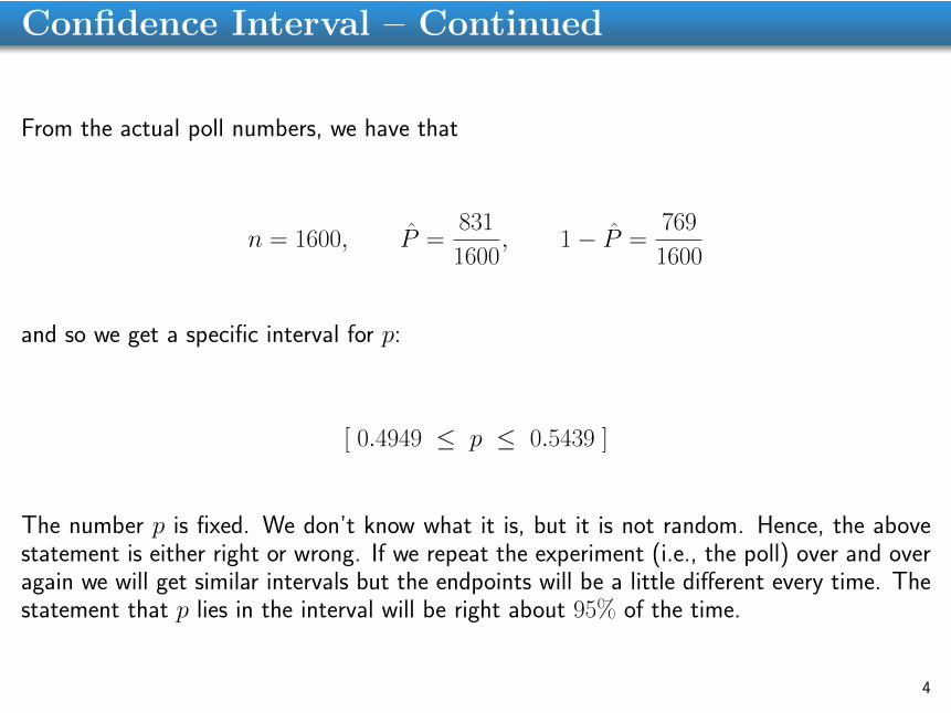
Confidence Interval – Continued

From the actual poll numbers, we have that

n = 1600, P̂ =831

1600, 1− P̂ =

769

1600

and so we get a specific interval for p:

[ 0.4949 ≤ p ≤ 0.5439 ]

The number p is fixed. We don’t know what it is, but it is not random. Hence, the abovestatement is either right or wrong. If we repeat the experiment (i.e., the poll) over and overagain we will get similar intervals but the endpoints will be a little different every time. Thestatement that p lies in the interval will be right about 95% of the time.

4

Confidence Intervals – Picking n

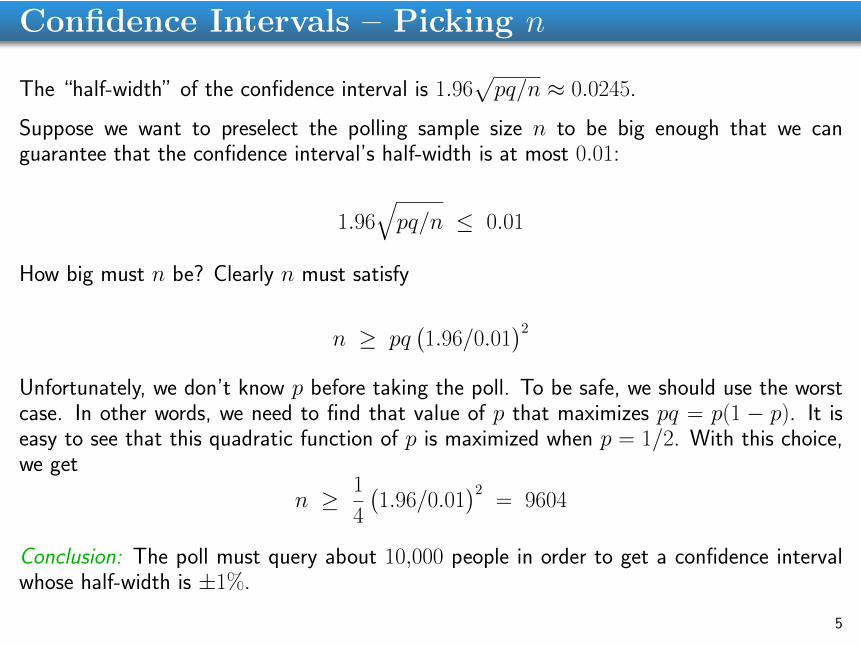
The “half-width” of the confidence interval is 1.96√pq/n ≈ 0.0245.

Suppose we want to preselect the polling sample size n to be big enough that we canguarantee that the confidence interval’s half-width is at most 0.01:

1.96√pq/n ≤ 0.01

How big must n be? Clearly n must satisfy

n ≥ pq(1.96/0.01

)2Unfortunately, we don’t know p before taking the poll. To be safe, we should use the worstcase. In other words, we need to find that value of p that maximizes pq = p(1 − p). It iseasy to see that this quadratic function of p is maximized when p = 1/2. With this choice,we get

n ≥ 1

4

(1.96/0.01

)2= 9604

Conclusion: The poll must query about 10,000 people in order to get a confidence intervalwhose half-width is ±1%.

5

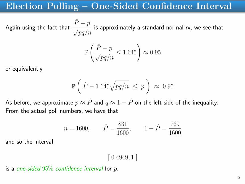
Election Polling – One-Sided Confidence Interval

Again using the fact thatP̂ − p√pq/n

is approximately a standard normal rv, we see that

P

(P̂ − p√pq/n

≤ 1.645

)≈ 0.95

or equivalently

P(P̂ − 1.645

√pq/n ≤ p

)≈ 0.95

As before, we approximate p ≈ P̂ and q ≈ 1− P̂ on the left side of the inequality.

From the actual poll numbers, we have that

n = 1600, P̂ =831

1600, 1− P̂ =

769

1600

and so the interval

[ 0.4949, 1 ]

is a one-sided 95% confidence interval for p.

6

A “Better” Confidence Interval

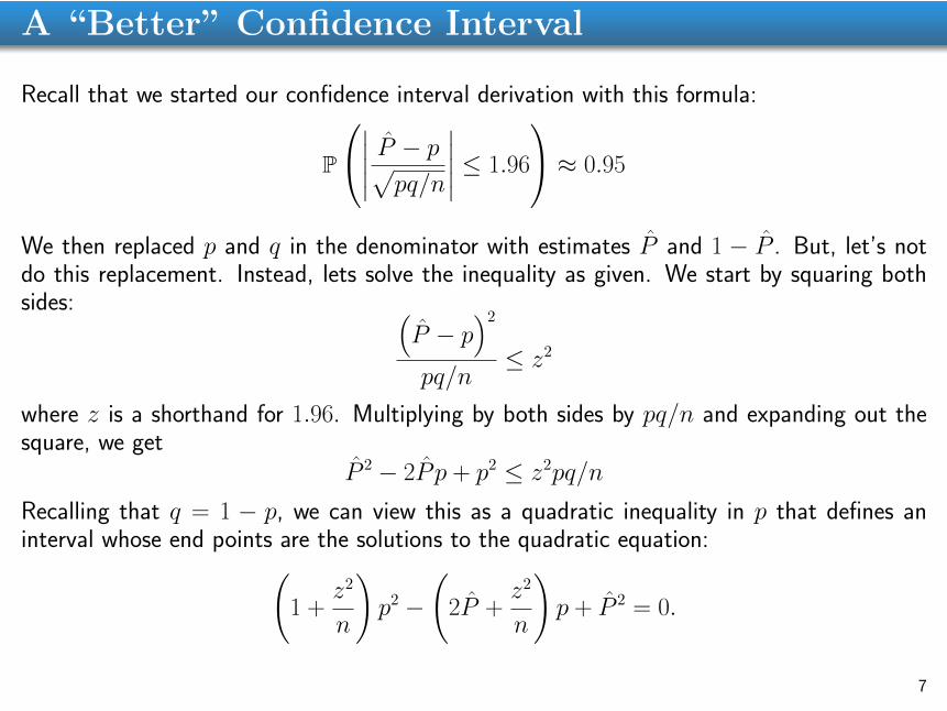
Recall that we started our confidence interval derivation with this formula:

P

∣∣∣∣∣ P̂ − p√pq/n

∣∣∣∣∣ ≤ 1.96

≈ 0.95

We then replaced p and q in the denominator with estimates P̂ and 1 − P̂ . But, let’s notdo this replacement. Instead, lets solve the inequality as given. We start by squaring bothsides: (

P̂ − p)2

pq/n≤ z2

where z is a shorthand for 1.96. Multiplying by both sides by pq/n and expanding out thesquare, we get

P̂ 2 − 2P̂ p + p2 ≤ z2pq/n

Recalling that q = 1 − p, we can view this as a quadratic inequality in p that defines aninterval whose end points are the solutions to the quadratic equation:(

1 +z2

n

)p2 −

(2P̂ +

z2

n

)p + P̂ 2 = 0.

7

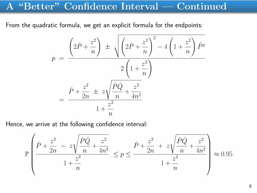
A “Better” Confidence Interval — Continued

From the quadratic formula, we get an explicit formula for the endpoints:

p =

(2P̂ +

z2

n

)±

√√√√(2P̂ +z2

n

)2

− 4

(1 +

z2

n

)P̂ 2

2

(1 +

z2

n

)

=P̂ +

z2

2n± z

√P̂ Q̂

n+

z2

4n2

1 +z2

n

Hence, we arrive at the following confidence interval:

P

P̂ +

z2

2n− z

√P̂ Q̂

n+

z2

4n2

1 +z2

n

≤ p ≤P̂ +

z2

2n+ z

√P̂ Q̂

n+

z2

4n2

1 +z2

n

≈ 0.95

8

Confidence Intervals

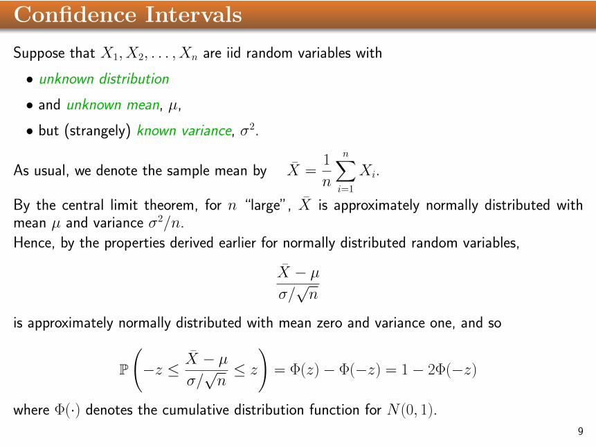
Suppose that X1, X2, . . . , Xn are iid random variables with

• unknown distribution

• and unknown mean, µ,

• but (strangely) known variance, σ2.

As usual, we denote the sample mean by X̄ =1

n

n∑i=1

Xi.

By the central limit theorem, for n “large”, X̄ is approximately normally distributed withmean µ and variance σ2/n.

Hence, by the properties derived earlier for normally distributed random variables,

X̄ − µσ/√n

is approximately normally distributed with mean zero and variance one, and so

P

(−z ≤ X̄ − µ

σ/√n≤ z

)= Φ(z)− Φ(−z) = 1− 2Φ(−z)

where Φ(·) denotes the cumulative distribution function for N(0, 1).

9

Confidence Intervals – Continued

For z = 1.96, we have Φ(−z) = 0.025 and therefore

P

(−1.96 ≤ X̄ − µ

σ/√n≤ 1.96

)= 0.95

The inequalities inside P(·) can be rearranged to read

P(X̄ − 1.96σ/

√n ≤ µ ≤ X̄ + 1.96σ/

√n)

= 0.95

In words, we say that there is a 95% chance that the true mean lies within 1.96 standarddeviations of the sample mean.

Since 1.96 is close to 2, it is common practice to report the X̄± 2σ/√n interval as the 95%

confidence interval.

10

Confidence Intervals – Continued

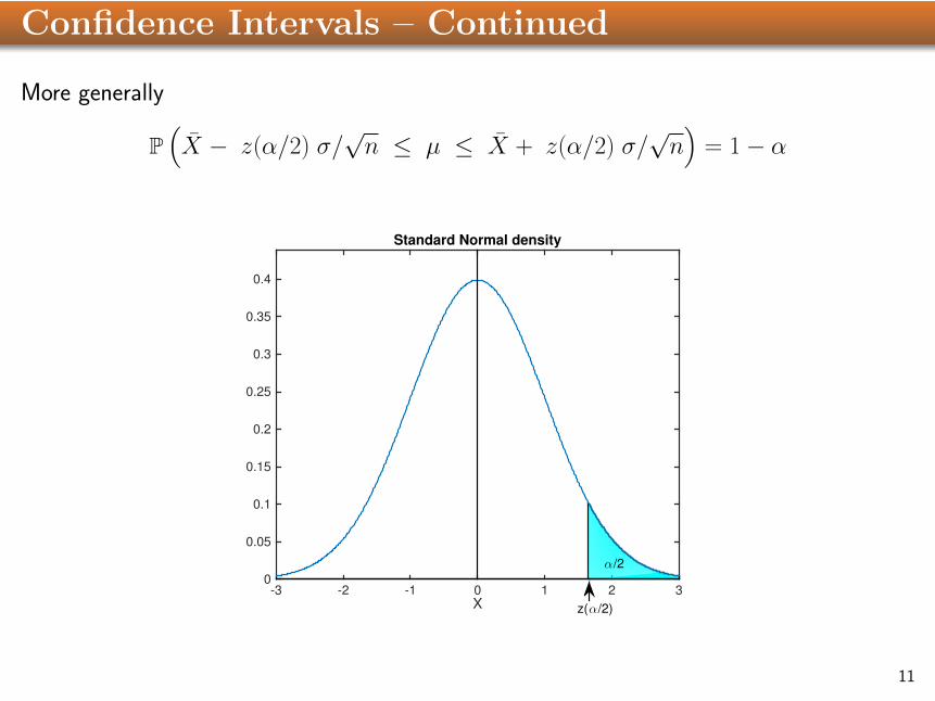
More generally

P(X̄ − z(α/2) σ/

√n ≤ µ ≤ X̄ + z(α/2) σ/

√n)

= 1− α

X-3 -2 -1 0 1 2 3

0

0.05

0.1

0.15

0.2

0.25

0.3

0.35

0.4

α/2

z(α/2)

Standard Normal density

11

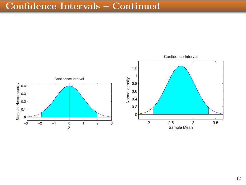
Confidence Intervals – Continued

−3 −2 −1 0 1 2 3

0

0.1

0.2

0.3

0.4

X

Sta

nd

ard

No

rma

l d

en

sity

Confidence Interval

2 2.5 3 3.5

0

0.2

0.4

0.6

0.8

1

1.2

Sample MeanN

orm

al density

Confidence Interval

12

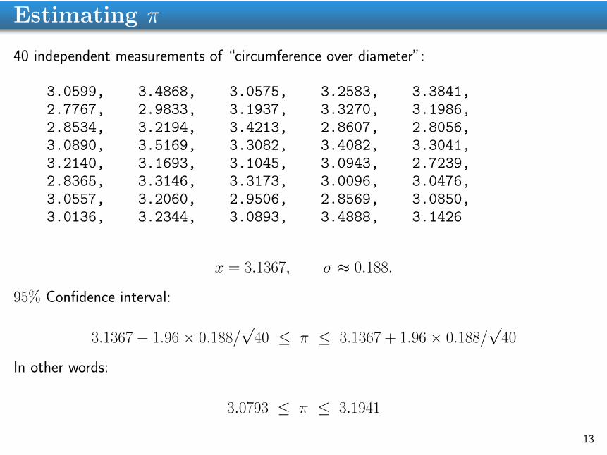
Estimating π

40 independent measurements of “circumference over diameter”:

3.0599, 3.4868, 3.0575, 3.2583, 3.3841,2.7767, 2.9833, 3.1937, 3.3270, 3.1986,2.8534, 3.2194, 3.4213, 2.8607, 2.8056,3.0890, 3.5169, 3.3082, 3.4082, 3.3041,3.2140, 3.1693, 3.1045, 3.0943, 2.7239,2.8365, 3.3146, 3.3173, 3.0096, 3.0476,3.0557, 3.2060, 2.9506, 2.8569, 3.0850,3.0136, 3.2344, 3.0893, 3.4888, 3.1426

x̄ = 3.1367, σ ≈ 0.188.

95% Confidence interval:

3.1367− 1.96× 0.188/√

40 ≤ π ≤ 3.1367 + 1.96× 0.188/√

40

In other words:

3.0793 ≤ π ≤ 3.1941

13

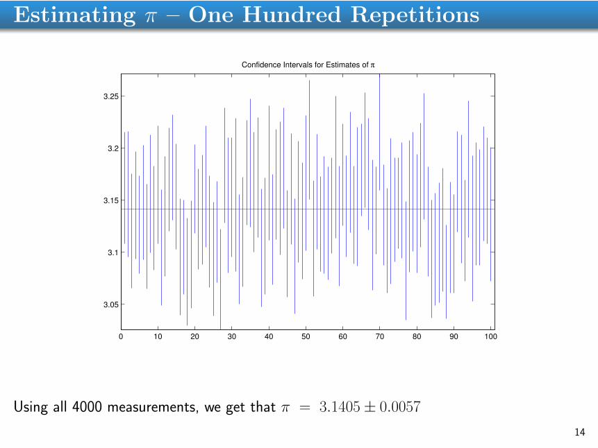
Estimating π – One Hundred Repetitions

0 10 20 30 40 50 60 70 80 90 100

3.05

3.1

3.15

3.2

3.25

Confidence Intervals for Estimates of π

Using all 4000 measurements, we get that π = 3.1405± 0.0057

14

Confidence Intervals – Unknown Variance

Usually the variance, σ2, is not known.In such cases, we approximate the variance by the sample variance

σ2 ≈ S2 =1

n− 1

n∑i=1

(Xi − X̄

)2The random variable

T =X̄ − µS/√n

has a t-distribution with parameter n.Hence, if we pick z so that F (z) = P(T ≤ z) = 0.975, then

P

(−z ≤ X̄ − µ

S/√n≤ z

)= F (z)− F (−z) = 0.95

And, therefore a 95% confidence interval for µ can be written as

P(X̄ − zS/

√n ≤ µ ≤ X̄ + zS/

√n)

= 0.95

Of course, the constant z depends on n. Values can be found in Table 4 of the textbook orusing Matlab’s tinv function. For large values of n, z ≈ 1.96.

15

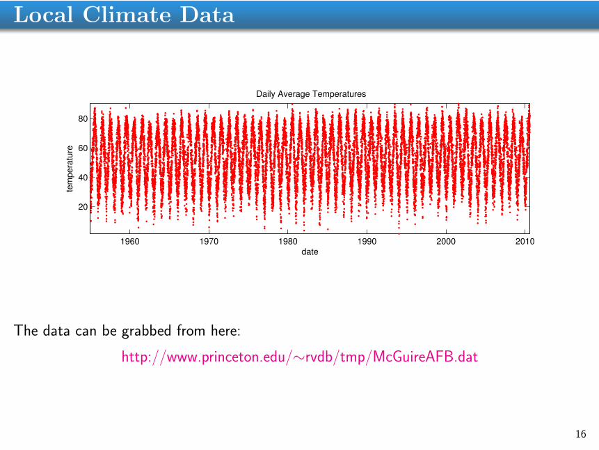
Local Climate Data

1960 1970 1980 1990 2000 2010

20

40

60

80

date

tem

pe

ratu

re

Daily Average Temperatures

The data can be grabbed from here:

http://www.princeton.edu/∼rvdb/tmp/McGuireAFB.dat

16

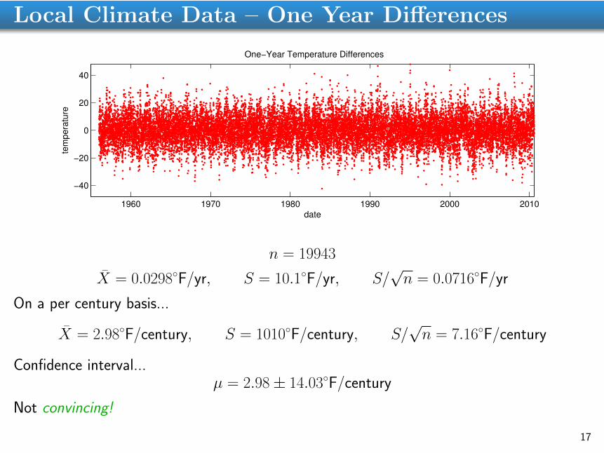
Local Climate Data – One Year Differences

1960 1970 1980 1990 2000 2010

−40

−20

0

20

40

date

tem

pera

ture

One−Year Temperature Differences

n = 19943

X̄ = 0.0298◦F/yr, S = 10.1◦F/yr, S/√n = 0.0716◦F/yr

On a per century basis...

X̄ = 2.98◦F/century, S = 1010◦F/century, S/√n = 7.16◦F/century

Confidence interval...µ = 2.98± 14.03◦F/century

Not convincing!

17

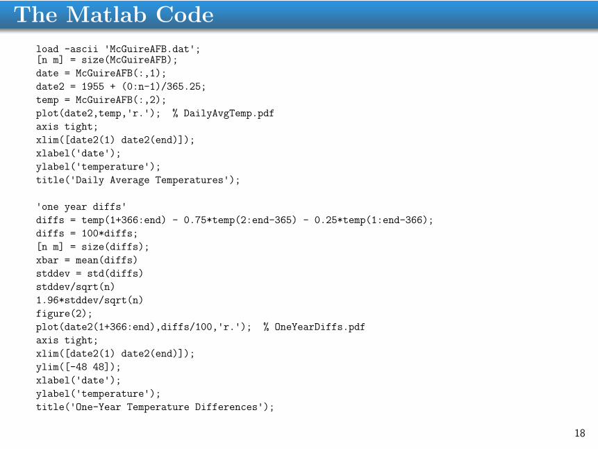
The Matlab Code

load -ascii 'McGuireAFB.dat';[n m] = size(McGuireAFB);

date = McGuireAFB(:,1);

date2 = 1955 + (0:n-1)/365.25;

temp = McGuireAFB(:,2);

plot(date2,temp,'r.'); % DailyAvgTemp.pdf

axis tight;

xlim([date2(1) date2(end)]);

xlabel('date');ylabel('temperature');title('Daily Average Temperatures');

'one year diffs'diffs = temp(1+366:end) - 0.75*temp(2:end-365) - 0.25*temp(1:end-366);

diffs = 100*diffs;

[n m] = size(diffs);

xbar = mean(diffs)

stddev = std(diffs)

stddev/sqrt(n)

1.96*stddev/sqrt(n)

figure(2);

plot(date2(1+366:end),diffs/100,'r.'); % OneYearDiffs.pdf

axis tight;

xlim([date2(1) date2(end)]);

ylim([-48 48]);

xlabel('date');ylabel('temperature');title('One-Year Temperature Differences');

18

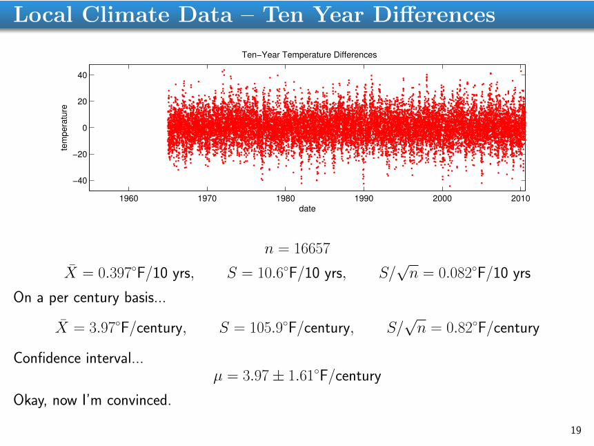
Local Climate Data – Ten Year Differences

1960 1970 1980 1990 2000 2010

−40

−20

0

20

40

date

tem

pe

ratu

reTen−Year Temperature Differences

n = 16657

X̄ = 0.397◦F/10 yrs, S = 10.6◦F/10 yrs, S/√n = 0.082◦F/10 yrs

On a per century basis...

X̄ = 3.97◦F/century, S = 105.9◦F/century, S/√n = 0.82◦F/century

Confidence interval...µ = 3.97± 1.61◦F/century

Okay, now I’m convinced.

19

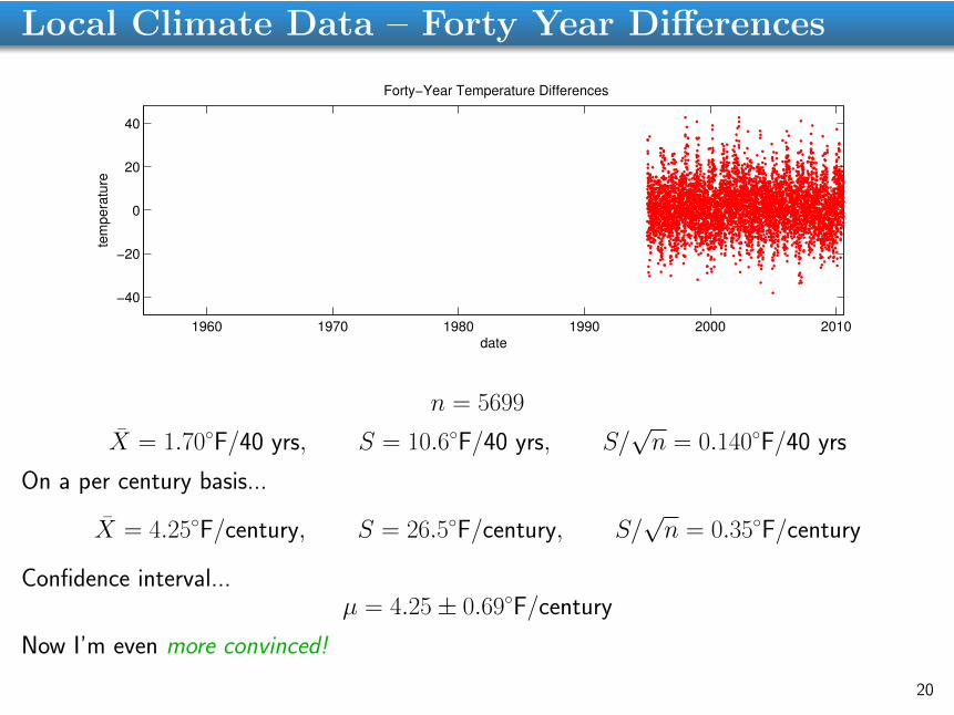
Local Climate Data – Forty Year Differences

1960 1970 1980 1990 2000 2010

−40

−20

0

20

40

date

tem

pera

ture

Forty−Year Temperature Differences

n = 5699

X̄ = 1.70◦F/40 yrs, S = 10.6◦F/40 yrs, S/√n = 0.140◦F/40 yrs

On a per century basis...

X̄ = 4.25◦F/century, S = 26.5◦F/century, S/√n = 0.35◦F/century

Confidence interval...µ = 4.25± 0.69◦F/century

Now I’m even more convinced!

20