Papadrakakis - Dynamic Relaxation

COMPUTER METHODS IN APPLIED MECHANICS AND ENGINEERING 25 (1981) 3548

@ NORTH-HOLLAND PUBLISHING COMPANY

A METHOD FOR THE AUTOMATIC EVALUATION OF THE DYNAMIC RELAXATION PARAMETERS

M. PAPADRAKAKIS

Institute of Structural Analysis and Aseismic Research, National Technical University, Athens, Greece

Received 26 November 1979 Revised manuscript received 6 March 1980

Dynamic relaxation, a vector iteration method which belongs to the family of methods under the title of three-term recursive formulae, is described with viscous and kinetic damping. An automatic procedure is developed for the evaluation of the iteration parameters, thus avoiding any trial run or any eigenvalue analysis of the modified stiffness matrix. Starting values for the maximum eigenvalue could be obtained from the Gershgorin bound, and for the minimum eigenvalue any positive number less than the estimated maximum eigenvalue. The method is applied to geometrically and material nonlinear problems, and comparisons are made with an improved conjugate gradient method and a direct stiffness method.

0. Introduction

Dynamic relaxation (DR) is based on the fact that a system undergoing dampted vibration, excited by a constant force, ultimately comes to rest in the displaced position of static equilibrium of the system under the action of the force.

In the majority of DR applications, in order to evaluate the iteration parameters, a trial run with zero damping is required until a periodic response of the total kinetic energy is observed. This procedure has the disadvantage of the uncertainty involved in knowing a priori the required running time with zero damping in order to develop a periodic response. Sometimes the number of iterations for the trial run needed to develop a periodic response exceeded the number of iterations required for the solution itself [l]. The only paper known to the writer where an on-going process was used for the estimation of the iteration parameters was that presented by Lynch et al. [2]. Starting with a rough estimate for the damping parameter, when a check on the curvatures of the deflection vector norm indicated an overdampted or an underdampted behavior, a change in the parameter was made. This process was used for linear plane stress problems only, and conclusions were uncertain to the extent that large adjust- ments could take the parameters beyond their optimum values and give inferior convergence to that of analyses using constant parameters.

In this paper a more general approach for the automatic evaluation of the DR parameters is developed which can guarantee convergence for almost any arbitrary initial estimate of the minimum and maximum eigenvalue of the modified stiffness matrix. The concept of kinetic damping is also examined with the same automated process as in the case of viscous damping. Numerical results for geometrically nonlinear structures and for path dependent problems are

36 M. Papadrakakis, A method for the automatic evaluation of the dynamic relaxation parameters

presented and comparisons are made with a conjugate gradient method and also a direct stiffness method for which the Newton-Raphson iteration technique is used.

1. Theoretical approach of DR

1 .l. Formulation of the iterative procedure

Let the system of equations for which a solution is sought be given by Kx = F with the solution x * = K-‘F. In order to achieve this solution by DR, the original equation is transformed into an equation of motion by introducing point masses and viscous damping forces at the nodes

M~+c~+KX=F, (1)

where M and C are the mass and damping diagonal matrices, respectively, and dots indicate differentiation with respect to time.

In the present analysis both mass and damping matrices are assumed to be proportional to the main diagonal terms of K: M = pD and C = CD. Eq. (1) is then integrated for displacement response under the load F until the system achieves a steady state equilibrium. With centred finite differences in time (1) may be discretized as

x *k+1’2 = (2 - ch/p)/(2 + ch/p)ik-l’* + (2h/p)/(2+ ch/p)D-‘[F - Kxk], (2)

where superscripts indicate time stations and h is the time step. Using the standard central finite difference for the relationship between displacements and velocities, the equation for x kC1 becomes

x k+l = Xk + j&+1/*. (3)

Eqs. (2) and (3) represent the iterative process of DR which may be classified as belonging to a general category of iterative methods, namely the ‘three-term recursive formulae’ [3].

1.2. Evaluation of the optimum iteration parameters

Lynch et al. transformed the iterative process into a standard eigenvalue problem for error vectors and examined quantitatively the convergence of the method. Under this approach the relationship between successive error vectors is given by

E lctl = [PI - yB]rk - aek-‘, (4)

where p = (2 - ch/p)/(2 + ch/p) + 1, y = (2h*/p)/(2 + chip), and B = D-‘K is the modified stiffness matrix. If the parameter A gives the rate at which the error vector decays with each iterative step, then

l k+’ = /Q,

where l k = xk -x*.

(5)

M. Papadrakakis, A method for the automatic evaluation of the dynamic relaxation parameters 37

Substitution of eq. (5) into eq. (4) gives

]](A LR - 'bRP + a)/(bRY)]l++ = 0, (6)

with (Y = /3 - 1. If Ag denotes one of the it eigenvalues of B, given by [AJ -B]e = o, then from eq. (6) comes the relation

GR - (p - ~/AJJ)A~R + cx = 0. (7)

For (p - yAs)/2 < & the roots of eq. (7) are complex; the modulus of ADR is independent of As and is given by

lADR ] = 6 = V(2 - ch/p)/(2 + chip).

For @ - yAB)/2 = fi the roots are real and equal, and

(8)

c2h2/p2 = ABh2/p(4 - ABh*/p). (9)

For (p - yAs)/2 > < the modulus of the larger of the two real unequal roots is given by

IJ~R(= ' 2 + chip [)2-n,h2/p[+ ,/y-?+$$I. (10)

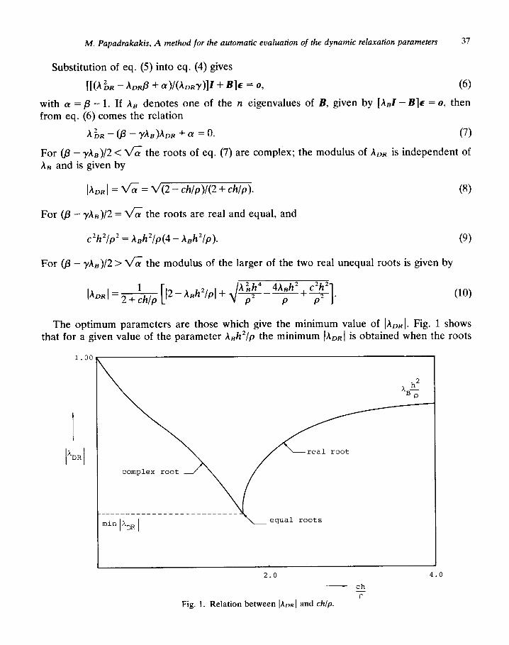
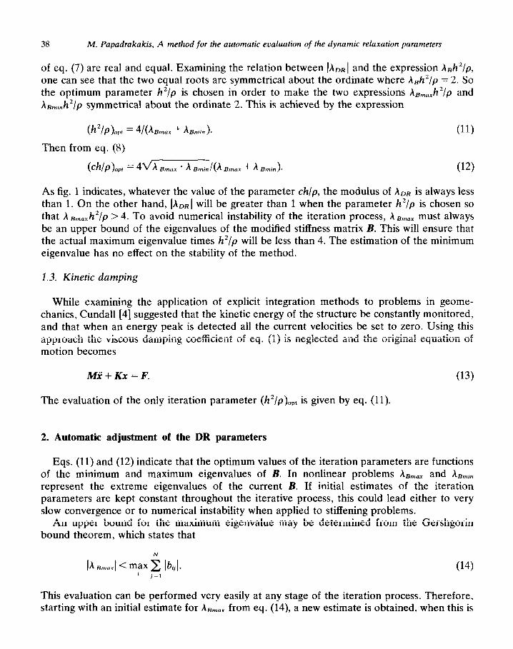
The optimum parameters are those which give the minimum value of ]hDR]. Fig. 1 shows that for a given value of the parameter ABh2/p the minimum ]hDR( is obtained when the roots

2.0 4.0

- ch

7 Fig. 1. Relation between IALIR 1 and chip.

38 h4. Papadrakakis, A method for the automatic evaluation of the dynamic relaxation parameters

of eq. (7) are real and equal. Examining the relation between [&I and the expression h,h2/p,

one can see that the two equal roots are symmetrical about the ordinate where h,h’/p = 2. So the optimum parameter h*/p is chosen in order to make the two expressions hsmaxh2/p and As,inh*/p symmetrical about the ordinate 2. This is achieved by the expression

(h2/p)opr = ~/(AB,,,+ Asmin ).

Then from eq. (8)

(11)

(chl&,t = 4dA ~max - A mninl(A ~max + A ~mm). (12)

As fig. 1 indicates, whatever the value of the parameter ch/p, the modulus of ADR is always less than 1. On the other hand, lADRI will be greater than 1 when the parameter h*/p is chosen so that A Bmaxh2/p > 4. To avoid numerical instability of the iteration process, ABmax must always be an upper bound of the eigenvalues of the modified stiffness matrix B. This will ensure that the actual maximum eigenvalue times h*/p will be less than 4. The estimation of the minimum eigenvalue has no effect on the stability of the method.

1.3. Kinetic damping

While examining the application of explicit integration methods to problems in geomechanics, Cundall [4] suggested that the kinetic energy of the structure be constantly monitored, and that when an energy peak is detected all the current velocities be set to zero. Using this approach the viscous damping coefficient of eq. (1) is neglected and the original equation of motion becomes

Mi+Kx =F. (13)

The evaluation of the only iteration parameter (h2/p)opt is given by eq. (11).

2. Automatic adjustment of the DR parameters

Eqs. (11) and (12) indicate that the optimum values of the iteration parameters are functions of the minimum and maximum eigenvalues of B. In nonlinear problems As,,, and Asmin represent the extreme eigenvalues of the current B. If initial estimates of the iteration parameters are kept constant throughout the iterative process, this could lead either to very slow convergence or to numerical instability when applied to stiffening problems.

An upper bound for the maximum eigenvalue may be determined from the Gershgorin bound theorem, which states that

IABmaxl<m;x~ Ibijl* (14) j=l

This evaluation can be performed very easily at any stage of the iteration process. Therefore, starting with an initial estimate for ABmax from eq. (14), a new estimate is obtained, when this is


necessary, either from eq. (14) with the current values of the matrix components bij or by increasing the previous estimate of ABmax by a certain amount according to the degree of nonlinearity of the problem. This adjustment may well be performed when a check on the curvatures of the residual vector norm or the velocity vector norm indicates the beginning of a numerical instability.

After establishing an upper bound for the maximum eigenvalue, an approximation to the minimum eigenvalue may be established as follows: Eq. (5) may be written in terms of successive correction vectors as

x k+l - Xk = A (x” _ Xk-l). (15)

A series of approximations to the dominant eigenvalue is then obtained by calculating the quotient

When the quantity given by eq. (16) has converged to almost constant value, it means that the dominant eigenvalue corresponds to the minimum eigenvalue which is given by the solution of eq. (7) with respect to hg:

hs = -(A ;R -ADRP +~)I@DRY). (17)

The above estimate of ABmin may then be used in eqs. (11) and (12) to evaluate the current optimum iteration parameters.

Current and optimum convergence rates Rutishauser [5] introduced the following convergence quotient for the Chebyshev methods:

e --O = (G - G)/(C + 62, (18)

where A,,, and Amin are upper and lower bounds of the eigenvalues of the modified stiffness matrix. The above expression is the same as that given in eq. (8) for the modulus of ADR. The optimum convergence rate is given by the value of the parameter w :

0 = -ln[(G - G)/(G + G)]. (19)

On the other hand, the expression -ln(A,R), with A DR obtained from eq. (16) is a measure of the current convergence rate of the iteration process. Thus, the value

0 = -ln(bR)/@

is an estimate of the ratio of current to optimal convergence rates. An update of the iteration


parameters is performed when A, has converged to a relative constant value and Q is subject to the condition 0 < 0 < 1.

3. Applications

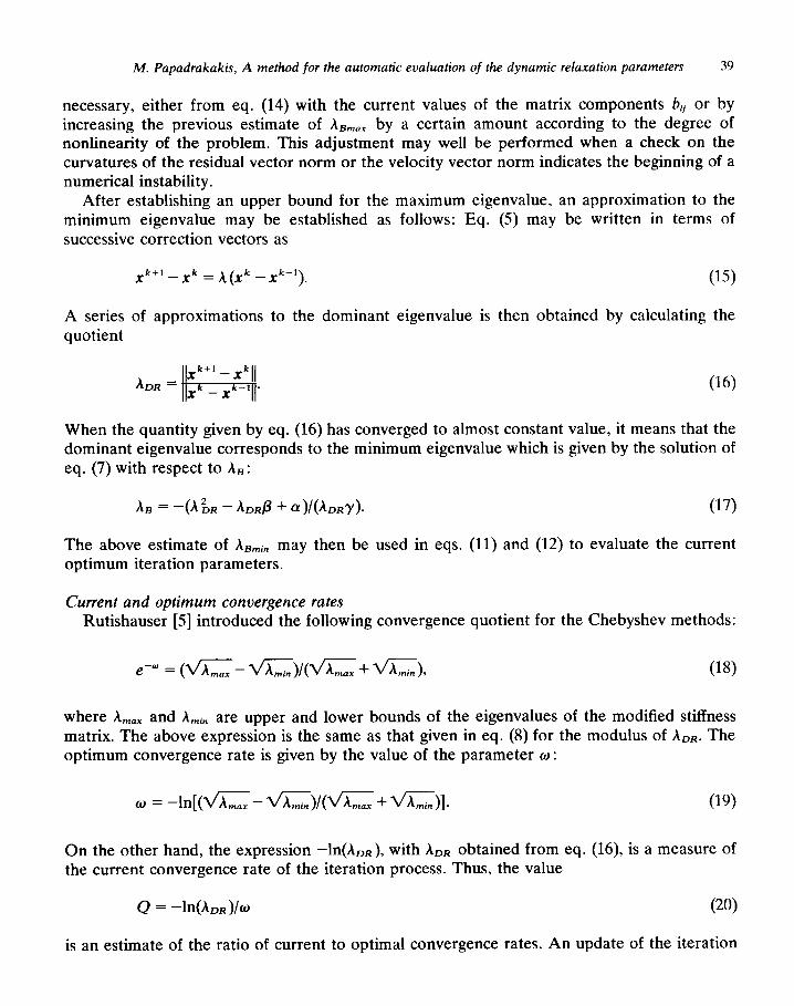
In order to demonstrate and compare the solution techniques, a pinjointed truss and three cable assemblies will be considered using finite element spatial idealizations. The pure iterative methods of dynamic relaxation and conjugate gradient perform the iterations from the original position to the final deflected position using the following equilibrium equations which cor- respond to an intermediate position:

i [2(x,, +x, -xc, -&A] + F,, = Rxq, I

i[gyt y, + YP - y, - Y,> 1

+ Fw = &7~

i[g(z,+r,-Zq-z,)]+F,,=R,,, I

(21)

where X,, Y,, Z, and x,, y,, z, are the initial coordinates and the displacements, respectively, of node p. The current length L can be expressed as

The final equilibrium position is attained when the residuals R become zero. The direct stiffness methods incorporate a Lagrangian formulation in which the elastic and

geometric stiffness matrices are considered [6].

:=‘\I / \ /P

’ ‘\ /

.\ \, ‘\ / /’ iSi

-X ‘\ _‘Lc ‘y’ /

I c ./

--- initial position

intermediate position

-'-'- final position

Fig. 2. Elements in space meeting at node q.


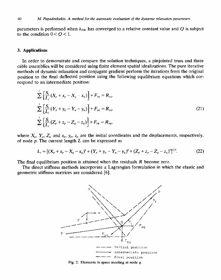
Table 1. Methods used for comparison

Abbreviated name Description of the method

DR DR with constant estimates for hBmox and hsrnin throughout the iteration process

DRAUT DR with automatic evaluation of the iteration

parameters

DRK DR with kinetic damping

CG The conjugate gradient method with the regula falsi- bisection algorithm for the one dimensional search

[71 NTRA Direct stiffness method with Newton-Raphson and a

semibandwidth storage scheme NTRAJE As NTRA with a compact storage scheme [8]

-

Table 2. Eigenvalue analysis of examples 1 and 2

Example 1

Initial configuration

Final configuration

Minimum Eigenvalue

O.l077E-01

O.l168E-01

Maximum Eigenvalue

2.1958

2.2123

Condition number

204

190

Initial Example 2 configuration 0.27368-03 2.1505 7860

Final

configuration O.l189E-02 2.2586 1900

In applying the various iterative methods to each example, iterations were continued until either the Euclidean norm of the residuals satisfies the error tolerance criterion E, IIRkII I E (RNORM criterion), or \l~“ll/ll~ll I E (QUOT criterion) where F is the current load vector. Table 1 shows the methods used and their abbreviated names. The vector iteration methods are diagonally scaled. The letters UNSC after the abbreviated name means an unscaled version of the method. In such cases B is reduced to the stiffness matrix and the mass and damping matrices are modified to M = pI and C = cl, respectively. In all test problems presented the effects of change of geometry are taken into account. The ultimate load-carrying capacity of examples 3 and 4 with combined geometric and material nonlinearities are also examined. All computer programs have been written in a similar way so as to permit reliable comparisons to be made. The computational work has been carried out on the CDC 7600 computer.

Example 1 A three-storey pin-jointed frame was analysed for a horizontal load at its uppermost node. From table 3 it may be seen that the number of iterations have been comparatively little

affected by different initial estimates of A,,, and Amin.


Table 3. Studies of example 1 with DRAUT (RNORM Table 4. Comparative study of example 1

criterion, E = O.lE-07) (RNORM criterion, E = O.lE-07)

Number of Initial Initial Convergence

iterations hmin mllx A tolerence for &JR Method

DR DRAUT DRK

Number of iterations Time (set)

166 0.182 98 0.129

180 0.190

127 1.0 2.22 O.lE-01

144 0.02 2.22 O.lE-01 128 0.02 2.22 O.lE-03 123 0.02 1.80 O.lE-01

121 0.1 1.80 O.lE-02

119 0.1 2.40 O.lE-02

98 0.1 2.22 O.lE-02

128 0.001 2.22 O.lE-02

Example 2 A counterstressed dual cable structure, which has also been analysed previously [9], [lo] has

been used as the second test problem. The evaluated minimum eigenvalue during the course of the iterative process is not always a

correct approximation of the actual current minimum eigenvalue. This could be explained by the fact that the initial estimate for the maximum eigenvalue differs from the actual current one. These differences could be quite substantial without deteriorating the convergence rate of the method to the same extent. From table 5 it may be seen that smaller initial estimates for A max produced better convergence rates because an underdamped behaviour is developed which accelerated the convergence in the early stages.

From table 6 it may be seen that DRAUT is faster than the other vector methods but considerably slower than the direct stiffness methods. This happens because this example has the minimum possible bandwith with a small number of zero elements inside the bandwidth.

Table 5. Studies of example 2 with DRAUT (RNORM

criterion, E = O.lE-05)

Number of Initial Initial Convergence iterations A m*n A rnllX tolerence for ADR

888 0.1 2.8736 O.lE-03 941 10.0 2.8736 O.lE-03 607 0.01 2.8736 O.lE-03 530 0.1 2.60 O.lE-02 688 0.1 2.60 O.lE-03 511 0.1 2.60 O.lE-04 533 0.1 1.80 O.lE-04 532 0.1 1.70 O.lE-04 569 0.1 1.50 O.lE-04 654 0.1 1.20 O.lE-04 560 0.1 1.00 O.lE-04


Table 6. Comparative study of example 2 (RNORM criterion, E = O.lE- 07)

Method DRAUT DRK CG NTRA NTRAJE

Time

(set) 0.725 0.916 0.905 0.105 0.145

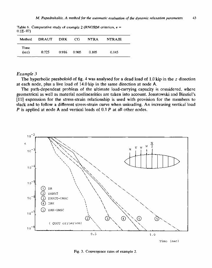
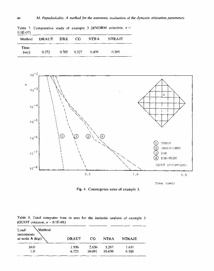
Example 3 The hyperbolic paraboloid of fig. 4 was analysed for a dead load of 1.0 kip in the z direction

at each node, plus a live load of 14.0 kip in the same direction at node A. The path-dependent problem of the ultimate load-carrying capacity is considered, where

geometrical as well as material nonlinearities are taken into account. Jonatowski and Birstiel’s [ll] expression for the stress-strain relationship is used with provision for the members to slack and to follow a different stress-strain curve when unloading. An increasing vertical’ load P is applied at node A and vertical loads of 0.1 P at all other nodes.

E

1 o-

1 o-

1 o-

1 o-

1 o-

1 o-

6

,8 ( QUOT criterion)

&,, (&, '\ '\

\ '\

'\ \ '\..

0.5 1.0

Time (set)

Fig. 3. Convergence rates of example 2.


Table 7. Comparative study of example 3 (RNORM criterion. 6 = O.lE-07)

Method DRAUT DRK CG NTRA NTRAJE

Time

(set) 0.372 0.705 0.527 0.439 0.285

1 o-;

E

, o-:

1 o+

1 o-5

10-j

1 o-’

1 o-8

‘\ ‘N \ \ .\ 0 DRALJT

\

4. 0 2 DRAUT-UNSC

'\ \ 3 DRK

'\ \ .'\ ..

0 '\

‘\

\ 0 4 DRK-UNSC

\', \'

(QUOT criterion) .\

0.5 1.0 1.5

Time (set)


Table 8. Total computer time in sets for the inelastic analysis of example 3

(QUOT criterion, E = O.lE-01)

DRAUT CG NTRA NTRAJE

10.0 1.936 2.636 3.267 1.631 1.0 6.723 10.091 10.670 6.105


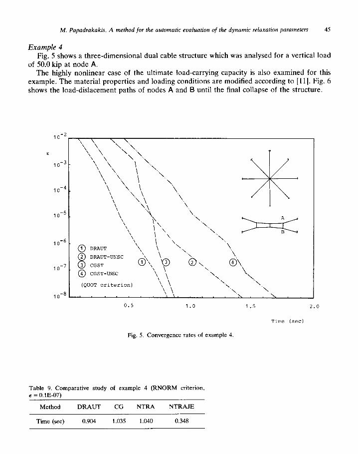
Example 4 Fig. 5 shows a three-dimensional dual cable structure which was analysed for a vertical load

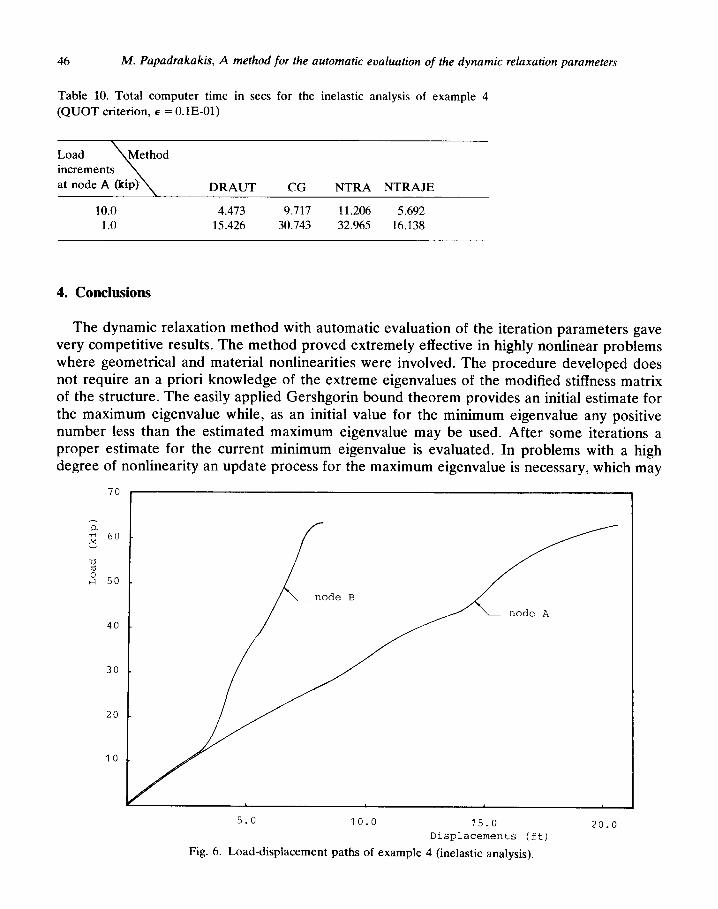
of 50.0 kip at node A. The highly nonlinear case of the ultimate load-carrying capacity is also examined for this

example. The material properties and loading conditions are modified according to [ll]. Fig. 6 shows the load-dislacement paths of nodes A and B until the final collapse of the structure.

lo-* , \ 1 \ 1 \ \ ‘\.

E ‘\ 1. y\.,

\ 1o-3 - \ ‘.

\ ‘.. \ \ ‘. \ ‘.. \ 1. \ 1.

\ ‘..\ \

\ \ “\ 1o-4 - ‘\, ‘\.\ 1, “\

\ “\ \ \ ‘1. \ “\ lo+ . \ ‘.\ \ \ \ “\

\ i\., “\ \ \ \ ‘\

“\ \ \ “\ x

lO+j. \ \ “1..

0 \

DRAUT '1

I ‘.\\ \ \

.\ 2 DRAUT-UNSC

8 3 CGST

10-7. 0

&,,, 'y 'b,.,

"\

@\

4 CGST-UNSC

(QUOT criterion)

lo-*- ’ ’

0.5

'\ \ '\ .\

\\

'\ \ "\

'\ \ '1.

1. "\ \ ,

1.0 1.5 2.0

Time (set)


Table 9. Comparative study of example 4 (RNORM criterion, E = O.lE-07)

Method DRAUT CG NTRA NTRAJE

Time (set) 0.904 1.035 1.040 0.348


Table 10. Total computer time in sets for the inelastic analysis of example 4

(QUOT criterion, l = O.lE-01)

Load Method increments

\ at node A (kip) DRAUT CG NTRA NTRAJE

10.0 4.473 9.717 11.206 5.692

1.0 15.426 30.743 32.965 16.138

4. Conclusions

The dynamic relaxation method with automatic evaluation of the iteration parameters gave very competitive results. The method proved extremely effective in highly nonlinear problems where geometrical and material nonlinearities were involved. The procedure developed does not require an a priori knowledge of the extreme eigenvalues of the modified stiffness matrix of the structure. The easily applied Gershgorin bound theorem provides an initial estimate for the maximum eigenvalue while, as an initial value for the minimum eigenvalue any positive number less than the estimated maximum eigenvalue may be used. After some iterations a proper estimate for the current minimum eigenvalue is evaluated. In problems with a high degree of nonlinearity an update process for the maximum eigenvalue is necessary, which may

70

a 2 60 .

2

s 50 .

5.0 10.0 15.0 Displacements (ft)

Fig. 6. Load-displacement paths of example 4 (inelastic analysis).


be performed by reapplying the Gershgorin bound theorem with the current values of the stiffness matrix components.

The use of kinetic damping instead of viscous damping simplifies the method, since only a bound for the maximum eigenvalue is necessary, but it gives inferior convergence rates to the viscous damping version.

References

[l] A.C. Cassell and R.E. Hobbs, Dynamic relaxation, Proceedings of IUTAM Symposium on High Speed Computing in Elastic Structures (Univ. Liege, 1970).

[2] R.D. Lynch, S. Kelsey and H.C. Saxe, The application of DR to the finite element method of structural analysis, Tech. Report No. THEMIS-UND-68-l (Univ. Notre Dame, Sep. 1968).

[3] M. Papadrakakis, Methods with three-term recursion formulae for the analysis of cable structures, Proceedings of IASS World Congress on Shell and Spatial Structures, Madrid, (Sep. 1979).

[4] P.A. Cundall, Explicit finite difference methods in geomechanics, Proceedings of E.F. Conference on

Numerical Methods in Geomechanics, (Jun. 1976). [5] M. Engeli, T. Ginsburg, H. Rutishauser and E. Stiefel, Refined iterative methods for computation of the

solution and the eigenvalues of self-adjoint boundary value problems (Birkhauser, Basel/Stuttgart, 1959). [6] J.H. Argyris and D.W. Scharpf, Large deflection analysis of prestressed networks, J. Struct. Div. ASCE (1972)

633-654.

[7] L.A. Schmit, E.L. Stanton, W. Gibson and G.G. Goble, Developments in discrete element finite deflection structural analysis by function minimization, Report AFFDL-TR-68-126 (Air Force Flight Dynamics Labora- tory, Air Force Wright Patterson Base, Ohio, Sep. 1968).

[8] A. Jennings, A compact storage scheme for the solution of symmetric linear simultaneous equations, Comp. J. 9 (1966) 281-285.

[9] H.A. Buchholdt, Pretensioned cable girders, Proc. ICE 45 (1970) 453-469. [lo] T.M. Murrey and N. Willems, Analysis of inelastic suspension structures, J. of Struct. Div. ASCE 97 (1971)

2791-2805. [ll] J.J. Jonatowski and C. Birnstiel, Inelastic stiffened suspension space structures, J. Struct. Div. ASCE 96 (1970)

1143-1166. [12] M. Papadrakakis, Gradient and relaxation nonlinear techniques for the analysis of cable supported structures,

Ph.D. Thesis, The City University, London (1978). [13] J.J. Jonatowski, Tensile roof structures: An inelastic analysis, International Conference on Tension Roof

Structures (PCL, London, 1974).

[14] J.S. Brew and D.M. Brotton, Nonlinear structural analysis by dynamic relaxation, Int. J. Numer. Meths. Eng. 3. (1971) 46M83.

[15] I. Davidson, The analysis of cracked structures, Trans. 3rd International Conference on Structural Mechanics and in Reactor Technology 3, part H (1975).

[16] D.A. Flanders and G. Shortley, Numerical determination of fundamental modes, J. Appl. Phys. 21 (1950) 1326-1332.

[17] I. Fried, Bounds on the external eigenvalues of the finite element stiffness and mass matrices and their spectral condition number, J. Sound and Vibration 22 (1972) 407418.

(181 J.W. Bunce, A note on the estimation of critical damping in DR, Int. J. Numer. Meths. Eng. 4 (1972) 301-304. [19] A.C. Cassell, P.J. Kinsey and D.J. Sefton, Cylindrical shell analysis by dynamic relaxation, Discussion, proc.

ICE (Jun. 1968) 241-250. [20] A.C. Cassel and R.E. Hobbs, Numerical stability of dynamic relaxation of nonlinear structures, Int. J. Numer.

Meths. Eng. 10 (1976) 1407-1410. [21] L.A. Hageman, The estimation of acceleration parameters for the Chebyshev polynomial and the SOR

methods, WAPD-TM-1038 (Jun. 1972).


[22] W.R. Hodgins, On the relation between DR and semi-iterative matrix methods, Numer. Math. 9 (1967) 446-451.

1231 K.R. Rushton, Dynamic relaxation solutions of elastic-plate problems, J. Strain Analysis 3 (1968) 23-32.

[24] M.R. Barnes, B.H.V. Topping and D.S. Wakefield, Aspects of form-finding using dynamic relaxation, International Conference on Slender Structures, London, (Sep. 1977).

[25] H. Wozniakowski, Numerical stability of the Chebyshev method for the solution of large linear systems, Numer. Math. 28 (1977) 191-209.

Documents

Papadrakakis - Dynamic Relaxation