Parallel algorithms for separable permutations

Discrete Applied Mathematics 146 (2005) 343–364

www.elsevier.com/locate/dam

Parallel algorithms for separable permutations

V.Yugandhar1, Sanjeev Saxena2

Department of Computer Science and Engineering, Indian Institute of Technology, Kanpur 208 016, India

Received 30 November 1999; received in revised form 20 September 2004; accepted 12 October 2004Available online 15 December 2004

Abstract

In this paper, it is shown that on the CREW model we can test whether a given permutation of1, . . . , n is separable in O(log n) time withn processors. Ifd is the depth of the optimal (minimum)depth separating tree of a separable permutation, then a separating tree of depth�(d) can be con-structed on the CREW model in O(log n) time with O(n2) cost or alternatively in O(d log n) timewith O(nd) cost. We can test whether the given separable permutationP of 1, . . . , k has a match in apermutationT of 1, . . . , n (n�k) in O(d log n) time with O(kn4) cost (the same as that of the serialalgorithm). We can also find the number of matches ofP in T in O(d log n) time with O(kn6) cost(the same as that of the serial algorithm). Both algorithms are for the CREWmodel. We also discusshow the space complexity of the existing serial algorithms for the decision problem can be reducedfrom O(kn3) to O(n3 log k) and of the counting version from O(kn4) to O(n4 log k).© 2004 Elsevier B.V. All rights reserved.

Keywords:Parallel algorithms; Separable permutations; Pattern matching; Tree traversal

1. Introduction

In the pattern matching problem for permutations we are given a permutationT=(t1, t2, . . ., tn) of 1, . . ., n,whichwecall thetext, andapermutationP=(p1, p2, . . ., pk)of 1, . . . , k, k�n, which we call thepattern. We wish to know whether there is a lengthksubsequence ofT, sayT ′ = (ti1, ti2, . . . , tik ), with i1< i2< · · ·< ik, such that the elements

1Now with: Synopsys Inc, 700 E, Middle Field Road, Mountain View, CA 94043, USA.2A significant portion of this work was donewhile this author was at Indian Institute of Information Technology

& Management, Gwalior, India.

E-mail address:[email protected](S. Saxena).

0166-218X/$ - see front matter © 2004 Elsevier B.V. All rights reserved.doi:10.1016/j.dam.2004.10.004

http://www.elsevier.com/locate/dam

mailto:[email protected]

344 V. Yugandhar, S. Saxena / Discrete Applied Mathematics 146 (2005) 343–364

of T ′ are ordered according to the permutationP, i.e., tir < tis iff pr <ps . This problemwas proposed by Herb Wilf[9,14].If Tdoes contain such a subsequence, wewill say thatT contains P, or thatPmatches into

T. For example, ifP is(1,2, . . . , k), thenwehave to findan increasing subsequenceof lengthk in T. The general problem is known to be NP-complete[9]. There are polynomial timealgorithms for the decision and the corresponding counting problem whenP is separable,i.e., contains neither the sub-pattern(3,1,4,2) nor its reverse, the sub-pattern(2,4,1,3)[9,14].The number of matches ofP into T can be counted in O(kn6) time using O(kn4) space

[9], given thatP is separable. The subproblems at an internal node can be solved from thesubproblems for its children. Ibarra[14] discusses the decision problem and shows thatit can be solved in O(kn4) time and O(kn3) space. In this paper we show that both thesealgorithms can be parallelized to run in O(d log n) time on CREW model with same costas that of the serial algorithms; hered is the depth of an optimal separating tree forP.Separable permutations can be viewed as permutations sortable in a particular way. This

is somewhat analogous to the characterization by Knuth[16] that permutations withoutthe pattern(2,3,1) are exactly the permutations sortable using one stack. Separable per-mutations are exactly the permutations that can be sorted in the following way. Imaginea straight segment of railway track, with the elements of the permutation lined up on thetrack, uncoupled, so that any element can be moved back and forth though without chang-ing the relative ordering of the elements. Imagine a segment in the middle of the trackthat can be rotated 180◦, thus reversing the order of the elements on the middle segment.Using this device, we may move any consecutive subsequence of the elements onto themiddle of the section of the track and reverse their order. There is one restriction: a se-quence of elements to be rotated on the middle section of the track must first be coupledtogether and must remain coupled forever afterwards. Separable permutations are exactlythe permutations that can be sorted using this method. An efficient algorithm for sortingthis way is described below. This linear time algorithm[9] also provides a test if a per-mutationP is separable. The algorithm is: use a stackSwhose elements are subrangesl, l + 1, . . . , l + m of the range 1, . . . , k. In general, to add a ranger to S, see if the topelement ofSforms a larger range together withr, i.e., the union of the two sets of numbersis a range. If so, pop the top element ofS, form the combined range, and recursively add ittoS; and if not, then push the ranger ontoS. The algorithm proceeds by scanning throughP once, making each element ofS into a singleton range and adding that range toS, as justdescribed. If, at the end ofP the stackS contains a single range then the permutation isseparable, and otherwise it is not.P’s separating treeT can be easily recovered. We give anO(log n) timeparallel algorithmwithnprocessors to checkwhether thegivenpermutation isseparable.The above sequential algorithm has a disadvantage of generating a skew tree (not

generating the optimal “minimum depth” separating tree) which might be pathologicalwhen we try to parallelize the algorithms. So in this paper we also describe a parallel algo-rithm to find a separating tree of a separable permutationPwith depth of the same order asthat of the optimal separating tree. The tree can be constructed in O(log n) time with O(n2)cost or alternatively in O(d log n) time with O(nd) cost whered is the depth of optimaltree.

V. Yugandhar, S. Saxena / Discrete Applied Mathematics 146 (2005) 343–364 345

Notation for separable permutations and separating trees and the parallel model of com-putation used in this paper is discussed in Section 2; for a general introduction to parallelalgorithms, a good reference is the book by JáJá[15]. The problem of constructing an op-timal separating tree is discussed in Section 3 and the problem of testing whether a givenpermutation is separable is discussed in Section 4. Parallel solutions of the decision and thecounting versions of the pattern matching problem are discussed in Section 5.In the rest of this section we discuss a tree traversal technique for efficient use of space

in the sequential setting[1, pp. 561–565]for both the decision and the counting versions ofthe sequential pattern matchings for permutations problem; a similar idea is also used in[3,pp. 50–52]. Basically, assume that a nodeV is evaluated by recursively evaluating the leftand right children ofV. The subtree having more leaves is evaluated first. Assume withoutloss of generality that the left subtree has more leaves. After evaluating the left subtree, wecan reuse the same space to evaluate the right subtree, thus the space required will be that ofevaluating the left subtree. If however both subtrees have same number of leaves, then werequire an extra slot for storing the intermediate result. Observe that in the computation, theworst case occurs only when there are equal number of leaves on both sides; however in thiscase, the depth of the tree (assuming recursively, that all descendants have same number ofleaves in both subtrees) will be O(log n).As O(n3) space is required at every node in the algorithm for testing whether the given

separable permutationP of 1, . . . , k is present in permutationT of 1, . . . , n (n�k), thistechnique will reduce the space requirement to O(n3 log k) from O(kn3). Further in thealgorithm for counting the number of matches ofP in T, the space required at every nodeis O(n4); this technique will reduce the overall space used to O(n4 log k) from O(kn4).

2. Preliminaries

Recall that a patternP is said to beseparableif it contains neither the sub-pattern(3,1,4,2) nor the sub-pattern(2,4,1,3). A separating tree for a permutationP=(p1, p2, . . . , pk) of 1, . . . , k is a binary treeTwith leaves(p1, p2, . . . , pk) in that order,such that for each nodev, if the leaves of the subtree rooted atv arepi, pi+1, . . . , pi+j , thenthe set of numbers{pi, pi+1, . . . , pi+j } is asubrangeof the range 1, . . . , k, i.e., is of theform {l, l+1, . . . , l+m}, for somel,mwith 1� l�k,0�m�k− l. This subrange is calledthe rangeof the nodev. If v is a node of the tree with left childvl and right childvr thenthe above condition implies that either the range ofvl just precedes the range ofvr , or viceversa. In the first casev is called apositivenode, and in the second case anegativenode. Forbrevity, we usev tomean both a nodev and the sequence of leaves of the subtree rooted atv.

Lemma 1 (Bose et al.[9] ). A patternP = (p1, . . . , pk) is separable iff it has a separatingtree.

The separating tree need not be unique. For example, the permutation(4,5,3,1,2,6)has the two separating trees ((((4,5),3),(1,2)),6) and (((4,5),(3,(1,2))),6). Observe that everynode in a separating tree is of out degree 2 or 0. So if there aren leaves in a separating treethen there will ben−1 internal nodes thereby determining the number of nodes in the tree.


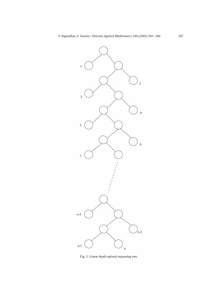
Lemma 2. There exists a separable permutation such that the depth of its optimal sepa-rating tree is�(n).

Proof. Letnbeeven.Consider theseparating treeof thepermutationP=(1,3,5,7, . . . , n−1, n, . . . ,8,6,4,2) (seeFig. 1). Observe that the separating tree for this permutation isunique and the depth of the tree isn− 1. For oddn a similar tree can be constructed.�

In this paper,weuse theparallel randomaccessmachine (PRAM)model. In thismodel, allprocessors execute the same instruction and communicate amongst themselves by readingand writing into the shared memory. In concurrent read exclusive write (CREW) model,processors can read from thesamememory cell simultaneously, however theprogramsaresowritten that they never attempt to write simultaneously in the same cell. In a concurrent readconcurrent write (CRCW) model, processors are allowed to write simultaneously into thesame cell. During concurrent write, in the tolerant CRCWmodel, the contents of the cell areunchanged. In common CRCW model, the program is so written that all processors tryingto write concurrently in the same cell, always try to write the same value, and that value getswritten. In arbitrary CRCW model, some processor is guaranteed to succeed. On all theseCRCW models, including tolerant[13, p. 90], the logical OR ofn bits can be computed inO(1) time withn processors. The algorithms in this paper only use this property of CRCWPRAMs; thus each CRCWmodel, as used in this paper, is basically the CREWmodel withadditional power to compute logical OR ofn bits in O(1) time. Thecostof an algorithm(or number of operations used) is defined to be the product of the number of processorsused and the time taken. A PRAMmodel is said to beself-simulatingif an algorithm whichtakest time with p processors can also be implemented on that model in O(rt) time withp/r processors; in other words, if instead ofp, onlyp/r processors are used, the time willincrease by O(r). The CREWmodel and all CRCWmodels (except tolerant are) known tobe self-simulating; the tolerant CRCW model is not known to be self-simulating. Supposethat an algorithm consists ofk parts and that parti, for i = 1, . . . , k can be implemented intime ti usingqi operations. If the PRAM is known to be self-simulating, then the algorithmcan be implemented in O(

∑ti ) time with O(

∑qi) operations[8, p. 32] (i.e., time and

operation counts are simultaneously additive). This can be seen as follows: parti can beimplemented withqi/piti processors in O(tipi) time, for pi�1, or in O(max{ti , qi/p})time with p processors. Thus withp =∑

qi/∑

ti processors, the entire algorithm willtake

∑O(max{ti , qi/p})=O(∑ ti )+O(∑ qi/p)=O(∑ ti )+ (1/p)∑(qi)=O(∑ ti )

time.We extensively use thisaccounting principlein analyzing algorithms; since the logicalOR ofnbits can be computed in O(r) time withn/r processors, the accounting principle isvalid for all algorithms discussed in this paper (even for the tolerant CRCW model, whichas used in this paper is basically the CREWmodel with additional ability to compute “OR”in O(1) time).

3. Construction of separating tree

We first explain how to test whether a given arraya[i..j ] which has distinct numbersfrom the set{1..n} forms a subrange (i.e., no gaps).


1

3

5

7

n-3

2

4

6

n-1n

n-2

Fig. 1. Linear depth optimal separating tree.


Step1: Find themaximum and theminimum of the arraya[i..j ]. These are rangeminimaand maxima queries[5]. Observe that all the elements of the arraya[i..j ] are in the range[1..n].Step2: Since there are no duplicates, if the difference between the maximum and the

minimum is equal to the difference betweeni and j thena[i..j ] forms a subrange of 1..notherwise not (pigeon hole principle[16]).Range minima queries take O(1) time with a single processor after O(n) preprocessing

cost[4,5]. The time taken for preprocessing is O(log log logn) on the CRCW PRAM[4]and O(log n) on the CREWPRAM[5]; n/ log log logn processors are used on the CRCWPRAM andn/ log n processors on the CREW model. Thus, in the above procedure, afterpreprocessing, both Step 1 and Step 2 take O(1) time with a single processor.We next describe a linear processor simple algorithm to test if a permutationP =

(p1, . . . , pn) is separable and construct a separating tree if one exists. Let the input permu-tation beP = (pi, . . . , pj ).Step1: For eachk(i�k�j), in parallel check if(pi, . . . , pk) forms one subrange and

(pk+1, . . . , pj ) forms another subrange of 1..n.Step2(a): If there is nok present for which we succeeded in Step 1 then stop. The

permutation is not separable.Step2(b): Else among the successfulk’s take the one which is nearest to(i + j)/2 as a

split pointS. Store the split pointSalong with the indices of the elements it split in a node.This will ensure that the number of leaves on each side will be roughly equal.Step3: Now recursively find the split points in childrenSl andSr in parallel of the

permutations(pi, . . . , pk) and(pk+1, . . . , pj ) and makeSl andSr point toS.Finding ak closest to(i+ j)/2 is either the closestk to the left of(i+ j)/2 or the closest

k to the right of(i+ j)/2.We look at these two values and see which is closer to(i+ j)/2.This is in effect finding the first one in a binary array which can be done in O(1) time on theCRCW PRAM see e.g.[12,5, p. 348]where it is referred to as “the 1-colour minimizationproblem”; the algorithm uses the fact that we can findOR ofnbits in O(1) time. First dividethe array into

√n parts and find OR of bits in each part. With(

√n)2= n processors we can

identify the first part which has a 1. Take this part (which has√n items), and again using

(√n)2= n processors, identify the first element with a one in that part.The split points along with the elements they split give a separating tree. As discussed

above, after preprocessing, Step 1 takes O(1) time on a CRCW PRAM. Further Step 2also takes O(1) time with linear number of processors. As the recursion depth is at mostd, the depth of the separating tree, we can construct a separating tree in parallel (afterpreprocessing) with linear processors in time proportional to the depth of the separatingtree; thus the algorithm will take O(d) time with n processors (see Theorem 1, first part).However, on the CREWmodel, withn/ log n processors each step will take O(log n) time,hence the total time taken on the CREWmodel will be O(d log n)with n/ log n processors(see Theorem 1, second part).In Step 2(b), what we are ensuring is that the number of leaves on either side of the

split point are as equal as possible. However, it is quite possible that one side may have asubtree which is unique and completely skewed. Thus, the depth by this method may not beminimal.Consider the followingseparablepermutation.(1,3,5,4,2,6,7,8,9,10,11,12),in Step 2(b), we will get the first split point between 6 and 7 and the separating tree as


(((1, ((3, (5,4)),2)),6), (((7,8),9), (10, (11,12)))) whereas the tree with the first splitpoint between 2 and 6((1, ((3, (5,4)),2))), (((6,7), (8,9)), (10, (11,12)))will have depthone less than the depth of our tree.However, there are certain observations which we can make.

Observation 1. In case there are two possible split pointsS1 andS2, hence two subrangessay[l, r], [r + 1,m] and[l, s], [s+ 1,m] then ifr < s then[l, r], [r + 1, s], [s+ 1,m] willalso be ranges and eitherS1 andS2will be both positive or will be both negative. Moreover,either

1. max[l, r]<min[r + 1, s] andmax[r + 1, s]<min[s + 1,m], or,2. min[l, r]>max[r + 1, s] andmin[r + 1, s]>max[s + 1,m].In fact, we can easily generalize to the following:

Observation 2. If [l, r] and[l, s] are both ranges,and ifr < s and exactly one of the largestor the smallest item in[l, s] is in [l, r] then[r + 1, s] is also a range.And also,

Observation 3. If [l, r] and [l, s] are both ranges, and if r < s and if [r + 1, s] is not arange, then[r + 1, t] is not a range for anyt�s.We next show that the depth of the tree constructed by our algorithm is of the same order

as that of the optimal separating tree.

Lemma 3. If d is the depth of the optimal separating tree, the tree constructed by ouralgorithm is of depth�(d).

Proof. We will use induction. Letd be the depth of the optimal separating tree and letd ′be the depth of the tree constructed by our algorithm.We will prove thatd ′�cd + c′ log nfor some constantsc andc′; note thatc�1. Asd =�(log n), the Lemma will then follow.All logarithms in the proof are to base 2.Assume that the claim is true for all ranges smaller thann. For the basis the claim is

clearly true forn�4. Let the split point in the optimal tree bek1. In case there are severaloptimal trees, we choose that optimal tree for which the split pointk1 is closest to themid-point. Assume, without loss of generality thatk1 is to the left of the mid-point i.e.,k1<n/2. Assume that the split point chosen by our algorithm isk2. First consider the casewhenk2>n/2. Letk3 be the position of the largest split point on the same side ask1 (i.e.,largest split point less thann/2). Clearlyk1�k3<k2. Observe that, there are no split pointsbetweenk3 andk2.Letn1 be the number of items to the left ofk1,n2 be the number of itemsbetweenk1 andk2

andn3 be the number of items to the right ofk2.Again, as our algorithmchoosesk2, we knowthatn1�n3. Letd ′L andd ′R be the depths ofTL the left andTR the right subtrees constructedby our algorithm and letdL anddR be the corresponding depths of the subtrees constructedby the optimal algorithm. Further, letd ′′L andd ′′R be the optimal depth of the left and right


subtrees, ifk2 is chosen as the split point. By induction hypothesis, we know thatd ′L �cd ′′L+c′ log(n1+n2)�cd ′′L+c′ log n andd ′R�cd ′′R+c′ log n3�cd ′′R+c′ log n.As the range forour right subtree[k2, n] ⊂ [k1, n], the range for the right subtreeof the optimal tree,d ′′R�dR.Now,d ′ =1+max{d ′L , d ′R}�1+max{d ′L , cd ′′R+ c′ log n}�1+max{d ′L , cdR+ c′ log n}.If d ′L �d ′R, thend ′�1+ cdR + c′ log n�c(1+ dR) + c′ log n�c(1+ max{dL , dR}) +c′ log n�cd + c′ log n and the proof will be complete. Hence, let us consider the casewhen the depth of the tree constructed by our algorithm is determined by the depth of theleft subtreeTL, and not by the depth of the right subtreeTR; thusd ′ = 1+ d ′L. The numberof leaves in the left subtreeTL will be n1+ n2.Case1: If n2<n3, then the number of nodes in the left subtreeTL is at most23 n, as in this

casen3 is larger than bothn1 andn2 andn=n1+n2+n3. Thus, an increase of the depth byone is “compensated” by the decrease in the number of leaves to be considered to two-thirds.Less informally,d ′ = 1+ d ′L �1+ cd ′′L + c′ log(n1+ n2)�1+ cd ′′L + c′ log(2n/3)�1+cd + c′ log(2n/3)�cd + c′ log n, for c′�2. Thus, the proof is complete by induction.Case2: If n2�n3, then asn3�n1, n1 is the smallest. By Observation 1[1 : k1], [k1+1 :

k3], [k3+1 : k2] and[k2+1 : n] are all ranges. In the left subtreeTL, k3 is again a candidatefor split point. It can be easily seen that in the left subtreeTL, there can be no split point tothe right ofk3 (i.e., betweenk3 andk2). Our algorithm will either choosek3 as a split pointor a point betweenk1 andk3 (asn1�n2). In case the depth of the tree is now determined bythe depth ofTLR, the right subtree ofTL, then it can be easily shown (by an argument similarto the one before Case 1) that the depth of our tree will be at most 2+ cdR+ c′ log n, andthe proof will be complete, withc�2. Hence, consider the case when the depth of the tree isdetermined byd ′LL , the depth ofTLL , the left subtree ofTL; the number of leaves inTLL , theleft subtree ofTL will be at mostn/2 (ask3 is to the left of the mid-point,k3<n/2). Here,an increase in the depth by two is compensated by the decrease in the number of leaves tobe considered to half. Less informally,d ′ = 1+ d ′L = 2+ d ′LL �2+ cd ′′LL + c′ log(n/2).Hered ′′LL is the depth of optimal separating tree over the same range asTLL . Observe thatd ′′LL �d. Thus,d ′�2+ cd + c′ log(n/2)�cd + c′ log n, asc′�2. Thus, the proof is againcomplete by induction.In casek1 andk2 are both on the same side (say both are on the left) of the mid-point,

then the number of nodes in that (left) subtree will be at mostn/2. Using the same notationas before, by inductiond ′L �cd ′′L + c′ log(n/2) = cd ′′L + c′ log n − c′�cd + c′ log n −c′�cd+c′ log n−1.As againk2>k1, sod ′′R�dR and hence,d ′R�cd ′′R+c′ log n�cdR+c′ log n�c(d −1)+ c′ log n�cd + c′ log n−1. Thus,d ′ =1+max{d ′L , d ′R}�1+ cd +c′ log n− 1= cd + c′ log n and the proof is again complete by induction as before.�

We next describe a faster algorithm using O(n2) processors. First initialize thearray[1..n,1..n] to zero. Then for each pair(i, j) check if (pi, . . . , pj ) is a range; if it is thenmakearray[i, j ] ← 1. Then by prefix sums we can easily get a sorted list of all orderedpairs (i, j) which form a range. Ifarray(i, k) and array(k + 1, j) are both 1 then ifarray(i, j) is also 1 then make(i, k) the left child and(k + 1, j) the right child of(i, j).Clearly this step can be implemented in O(1) time with O(n3) processors, we discuss theimplementation of this step with O(n2) processors later. If the separating tree is not unique,the graph will not be a tree; i.e., a node may have more than one parent. Some of the nodesmay not have any parents (possibly). In a sequential setting we can delete all these nodes


one by one (this may have cascading effect). Assuming that the permutation is separable aseparating tree is present in the directed acyclic graph.In a parallel setting, each node picks up the pair of left and right child for whichk is

most balanced. Each(i, j) searches for(i, k) in the sorted list of ordered pairs, wherekis the closest to(i + j)/2 among the elements in the positions between the smallest andlargest elements of[i, j ] (see Observation 2). Then make(i, k) the left child and(k+ 1, j)the right child of(i, j); each left child points to its right sibling and conversely; edges aredirected from children to parent; but the parent also stores the pair of left child and rightchild together with the corresponding valuek. Nodes not picked up do not have parentedges. As a result we are left with a collection of rooted trees. If we remove nodes fromwhich the root is no longer reachable we will be left with a separating tree. We can checkif the root is not reachable by pointer doubling. Actually in O(log n) time, we can also useparallel tree contraction[15] and the algorithmwill then take O(log n) time with cost linearin number of nodes which is O(n2) (see Theorem 1, third part).Recall thatarray(i, j) is 1, if and only if,(pi, . . . , pj ) is a range. Ifarray(i, k) and

array(k + 1, j) are both 1 and ifarray(i, j) is also 1 then we are required to make(i, k)the left child and(k + 1, j) the right child of(i, j). Let us now discuss implementation ofthis step with O(n2) processors. Observe that if[l, r] and[l, s] are both ranges withs > rthen using Observation 2, we first check if we can make[l, r] a left child and[r + 1, s] aright child of [l, s] (this involves a single range minima and range maxima query and canbe carried out with a single processor in O(1) time after preprocessing); if we cannot, thenby Observation 3,[l, r] cannot be a left child of any node. The next “1” in the same row,will help us getting the next sibling (these are in fact “is a prefix of” pointers). If we try tolook in the same column (upward) we get “is a suffix of” pointers. In case, if for a node,there are both pointers, then there is an ambiguity (or more than one tree is possible). Andwe can take either of them say, the one in the same row. Here we have to find all next (orprevious) positions of ones in a binary array i.e., create a chain or linked list of all indiceswhere the value is one. This can be easily computed by prefix maxima or even faster inO(�(n)) time [17,7]with linear processors.The complete implementation for this step is as follows. We first make a copy ofarray

[1..n,1..n] and call this copylef t_child[1..n,1..n]. First assign one processor to eachentry of array. If array(l, r) is one (i.e.,(l, r) is a range), lets be the next one in rowl (we have linked list of all ones in each row), if(r + 1, s) is not a range, then makelef t_child(l, r)= 0, otherwise makelef t_child(l, r)= r. From Observation 3, we knowthat (l, r) cannot be a left child if(r + 1, s) is not a range. This is done independently,in parallel, for each entry ofarray. Next assignn processors to each row oflef t_child,and in parallel, carry out the prefix maxima computation (for each row) and store the resultin the arraypref ix_maxima_lef t_child. In an arrayA[1 : n], the prefix minimas areB[i]=min{A[j ] : 1�j� i} and the suffix minima areC[i]=min{A[j ] : i�j�n}. Prefix(or suffix) minima (or maxima) can be found in O(log n) time on the CREW model[15]or in O(log log logn) time on a CRCW PRAM[4] with linear cost, in both cases. As aresult, ifpref ix_maxima_lef t_child(l, i) = k, we know that(l, k) is a range and(l, j)is not a range fork + 1�j� i. Finally, we assign one processor to each entry ofarray. Ifarray(i, j)= 1, then we findk=pref ix_maxima_lef t_child(i, (j + i)/2) we also findthe next one afterk, sayk′ in row i and choosek or k′ whichever is closer to(i + j)/2 (say


k) and make(i, k) the left child and(k + 1, j) the right child of(i, j), assuming of coursethatk �= 0.Summarizing the discussion together with that before Observation 1 and using Lemma

3, we have the following Theorem:

Theorem 1. If d is the depth of the optimal separating tree of a separable permutation thena separating tree of depth�(d) can be obtained in either:

1. O(d + log log logn) time on CRCW PRAM withO(nd) cost, or alternatively in2. O(d log n) time withO(nd) cost on CREW model, or alternatively in3. O(log n) time withO(n2) cost on CREW model.

Remark. If we allow the separating tree to have more than two children whenever thereare more than one possible values ofk, then in this case from Observation 1 (with threeor more children—viz., all minimal subranges), the tree will be unique. If[l, m] is a rangeat nodev and fork1<k2< · · ·<kr , [l, ki] and[ki + 1,m] are also ranges, then we makeranges[l, k1], [k1+1, k2], . . . , [ki+1, ki+1], . . . , [kr−1+1, kr ], [kr+1,m] all children of[l, m] (in this order). From the second part of Observation 1 (all children are either positiveor negative) we can convert this tree into binary tree by arbitrarily grouping contiguous setof children; if a node hasr children, then we can merge the range for firsti (for any i�1)for the left child and merge the range of remainingr − i for the right child. We conjecturethat by carrying out “height balancing” operations (or rotations) as we move up level bylevel (in parallel for all nodes at that level), the time taken will be O(d) and height will beoff by at most one (as in AVL trees).

4. Testing permutations for separability

In this section, we will describe parallel algorithms for testing whether a given permuta-tion is separable.WithO(n4)processors, for all length4subsequencesofPwecancheck inparallelwhether

they match with(2,4,1,3) or (3,1,4,2). If there is any match then the permutation is notseparable else the permutation is separable. The time taken is clearly O(1). Here a CRCWmodel is required as there may be concurrent writes if the permutation is not separable;there will be no concurrent writes if the permutation is separable.We next reduce the number of processors to O(n3). With O(n3) number of processors,

for all length 3 subsequences ofP check in parallel whether they match with(2,1,3) or(3,1,2). For each length 3 subsequence which matches with(2,1,3) or (3,1,2) find thelargest elementL, between the elements which match 1 and 2. Now check whether thislargest elementL is larger than all the matched elements corresponding to 1,2,3. If so thepermutation is not separable. If no suchL is found thenP is separable.Here also we are using range queries for each matching 3 tuple. Hence the time is

O(1) with a single processor after preprocessing. The time taken for preprocessing isO(log log logn) on a CRCW PRAM[4] and O(log n) on the CREW PRAM; the costis O(n) in both the cases. On a CRCW PRAM the preprocessing time can be reduced to


O(1) with O(n log3 n) = O(n2) processors[4]. As every length 3 subsequence is checkedin parallel, the number of processors used is O(n3).The processors can be easily reduced to O(n2) but the time, by the direct approach,

will become O(log n). Assume that we are testing for 2,4,1,3. Fix two items, say, theitems corresponding to 2 and 1. Find the range maxima between these items, the rangemaxima will correspond to 4. Check if there is any item on the right of the item which isfixed as 1 whose value lies between the values of the items matching with 2 and 4. Thiscan be tested by rectangular or orthogonal range queries (counting version). If there isany such item then the permutation is not separable. Else if there is no such item for allfixed combinations of 2 and 1 then the permutation is separable. The routine to test with3,1,4,2 is symmetric. Orthogonal range queries take O(log n) time (see e.g.[18, indirectretrieval]and[11, Cor 2]); note that we are essentially using sequential algorithm (i.e., withp = �(1)). This concludes the description of the algorithm that runs in O(log n) time withO(n2) processors on the CREW PRAM.The orthogonal range query is the bottleneck in the procedure. However, in orthogonal

range query, here we have to search over the suffix or the final portion (or prefix, the initialportion) of a permutation and for thesespecial orthogonal range querieswe can do better.Assume that in the pattern, numberpoccurs in theith place, thenmake INDEX[p]= i. Thusthe array INDEX will give the location where each number occurs. To answer orthogonalrange queries for suffix (respectively, prefix) preprocess the array INDEX for the rangemaxima (resp. minima) queries; preprocessing takes O(1) time with O(n log3 n) = O(n2)processors[4, Lemma 2.4]. If the orthogonal range query is(p, q), then the range maxima(resp. minima) over(p, q) in the array INDEX will give the location of the last (first) itembetweenpandq. The time for the query is O(1) with a single processor. This concludes thedescription of the algorithm that runs in O(1) time with O(n2) processors on the CRCWPRAM.Wefinally describeadivideandconquer algorithmwith linear processors.Assume thatwe

havedivided thearray into twoparts (not necessarily of samesize) andeachpart is separable.If the entire array is non-separable then all four items cannot come from the same part orgroup. Find the suffixmaximaand the suffixminima for the left groupandalso find theprefixminima and the prefix maxima for the right group. In an arrayA[1 : n], the prefix minimasareB[i] =min{A[j ] : 1�j� i} and the suffix minima areC[i] =min{A[j ] : i�j�n}.Prefix (or suffix) minima (or maxima) can be found in O(log n) time on the CREWmodel[15] with linear cost. Also assume that we have a sorted list of the items in both groups.A sorted list of items at each node can be obtained using Cole’s sort[10] in O(log n) timewith n processors on the CREW model.Case1: Three items are from the left group.Assume the items corresponding to 2,4,1

are in the left group and the item corresponding to 3 is in the right group.

Assume that we have fixed the item corresponding to 2. Use binary search on the suffixminima array (of the left group) to find the last item of the group which is smaller thanthe item corresponding to 2. That item will correspond to 1.

Find the range maxima between items corresponding to 1 and 2. It will correspondto 4.


Check whether any item is present in the right subgroup between items correspondingto 2 and 4; this can be done by binary search if the right group is sorted.

Thus for any item fixed as 2 we can check whether the prohibited pattern is present inO(log n) time with a single processor. We check for all the items in the left subgroup inparallel.Case2:Two items are from the left group.Assume the items corresponding to 2,4 are in

the left group and the items corresponding to 1,3 are in the right group.

If the item corresponding to 3 is fixed in the right group the item corresponding to 1is the smallest item to its left; this can be obtained from the prefix minima of the rightgroup in O(1) time.

Do binary search in the suffix maxima array of the left group to find the last item inthe left subgroup larger than the item corresponding to 3; this is item 4.

See if there is any item between items corresponding to 1 and 3 on the left of the itemcorresponding to 4 in the left subgroup.

The last step in Case 2 requires an orthogonal range query, but here we have to searchover the prefix or the initial portion. For thesespecial orthogonal range querieswhere wehave to search over the prefix or the suffix (the final portion), we can do better.While sortingthe right or the left part during the preprocessing stage, we also “remember” the originalindex or the position of the items. Next, again in the preprocessing stage, we create an arrayof indices. Thus ifA is the sorted array, and itemA[i] was injth position (before sorting)then in INDEX, the array of indices, INDEX[i] = j . To answer orthogonal range queriesfor suffix (resp. prefix), we preprocess the array INDEX for range maxima (resp. minima)queries. If the orthogonal query is(p, q), then we first locatepandq inA, say the positionsareip, iq such thatA[ip − 1]<p�A[ip] andA[iq ]�q <A[iq + 1]. Now range maxima(minima) over(ip, iq) on array INDEX will give the location of the last (first) item in therange (i.e., betweenp andq). Thus the time for query will be O(1) with a single processor(after binary search).Case3:One item is from the left group.Assume the item corresponding to 2 is in the left

group and items corresponding to 4,1,3 are in the right group.

Assume that we have fixed the item corresponding to 3 in the right group. Use binarysearch on the prefix maxima array of the right group to find the first item of the groupwhich is larger than the item corresponding to 3. That item will correspond to 4.

Find the rangeminima between items corresponding to 4 and 3. It will correspond to 1.

Check whether any item is present in the left subgroup between items correspondingto 1 and 3 (binary search if the left group is sorted).

Thus with linear number of processors on the CREW model, we can find whether thecombination of two separable permutations is separable or not in O(log n) time. The com-plete algorithm is as follows: divide the given permutationP into two halves, recursively


(in parallel) check each half for a non-separable permutation. If not found, see if the com-bination is separable or not. IfT (n) is the parallel time with linear number of processorsthe recurrence relation is:T (n) = T (n/2) + log n. The solution of which is O(log2 n).Thus with linear number of processors we can check in O(log2 n) time whether the givenpermutation is separable or not.

Lemma 4. Given a permutation, we can test whether it is separable with the following(time, processor) trade-offs:

(1, n2), (log n, n2), (log2 n, n).

The first trade-off is for a CRCW PRAM and last two are for the CREW PRAM.

Actually, we can reduce the time to O(log n) with n log n processors. Basically, weconstruct a binary tree overn leaves; at each level we assume that the permutation at leavesof both children are separable and check whether the combination is separable using theO(log n) timeCREWalgorithm.As at each level there aren items, the number of processorsused isO(n log n). In case the permutation is not separable, we set a local “flag”, and finally,take logical OR of these local flags, hence, concurrent writes are not required. Thus we havethe following:

Corollary 1. Given a permutation, we can test whether it is separable inO(log n) withn log n processors on a CREW PRAM.

We show in Corollary 2 below that after preprocessing, the computation time can bereduced to O(1) with n processors for each level of the binary tree andn log n processorsin all; we then reduce the number of processors tonby performing the computation for eachlevel in sequence, which increases the time to O(log n). This algorithm runs in O(log n)time withn processors on the CREW PRAM.

Corollary 2. Given a permutation, we can test whether it is separable inO(log n) with nprocessors on a CREW PRAM.

Proof. We assume, as part of preprocessing, that all sets have been preprocessed for rangemaxima and minima queries[5] and prefix and suffix maximas and minimas have beendetermined[15]; this will take O(log n) time with n processors, or with a processor-timeproduct of O(n log n).We also assume that we have a sorted list of items for both sets as forCorollary 1; this takes O(log n) time withn processors on the CREWmodel[10]; this alsoresults in processor-time product of O(n log n). By merging as part of preprocessing, wecan avoid doing binary search as follows[2, Lemma 2.1, p. 217], if we have to search (findthe correct position for) each item of the sorted arrayA in the sorted arrayB and we havethe array resulting from mergingA andB, then ifA[i] is in thekth position in the mergedarray, thenB[k − i]<A[i]<B[k − i + 1].As merge of two sorted arrays, each havingm items, can be easily done on CREWmodel

in O(log m) time withm/ log m processors[15], or with a processor-time product of O(m)results of all merges can be precomputed in O(log n) time, with a processor-time product


of O(n log n) (as there aren items at each level, processor-time product at each level isO(n)).Thus, the entire preprocessing takes O(log n) time with a processor-time product of

O(n log n) on the CREWmodel. Using the accounting principle, the time will be O(log n)with n processors on a CREW PRAM.Now, let us consider one case (say Case 1) of the algorithm in detail (the other cases are

similar):Case1: Three items are from the left group.Let us assume that as part of preprocessing

we have the result of merging the sorted left group and the suffix minima of the left group[6]. Each item (sayx) in turn is fixed as 2, and we are required to locatex in the suffixminima array; this can be done for eachx by a single processor in O(1) time and will givethe item corresponding to 1. Again we know the merge of the left and the right group. Asa result, we can find the item in the right group just larger thanx; this will correspond tothe item corresponding to 3. By a range maxima query (as before) we can locate the largestitem between items corresponding to 1 and 2 and compare this with the item correspondingto 3.Let us finally look at the “orthogonal range query” of Case 2. Array “INDEX” is created

as before. Now ifip andiq can be determined, then the final answer can be obtained by arange maxima (or range minima) query, as before. But as we know the merge of the leftand right sets,ip andiq will just be the positions of items corresponding to 1 and 3 in theleft group. �

Summarizing results of this section, we have

Theorem 2. Given a permutation, we can test whether it is separable with the following(time, processor) trade-offs:

(1, n2), (log n, n).

The first trade-off is for a CRCW PRAM and the second for the CREW PRAM.

5. Parallel algorithms for pattern matching problems

The input is a text permutationT = (t1, . . . , tn), a separable pattern permutationP = (p1 . . . , pk) and a separating tree forP. We will give two parallel algorithms to testwhetherPmatches intoT. For the first algorithm for every nodev of the tree we define thevaluesL(v, i, j, x) andH(v, j, k, x) for all 1� i�j�k�n,1�x�n, as follows[14].L(v, i, j, x) =max{{0} ∪ {y | there is a matchM of v into (ti , . . . , tj ) such thatM’ssmallest element isy andM’s largest element is less than or equal tox.}}.

L(v, i, j, x)>0 if and only if there is a match ofv into (ti , . . . , tj ) such that the match’selements are at mostxand furthermore,L(v, i, j, x) is the maximin match element over allsuch matches[14]. L(v, i, j, x) cannot decrease if we decreasei or increasej or increasex[14].


H(v, j, k, x)=min{{n+ 1} ∪ {y | there is a matchM of v into (tj , . . . , tk) such thatM’s largest element isy andM’s smallest element is greater than or equal tox.}}.Thus,H(v, j, k, x) is less thann+ 1 if and only if there is a match ofv into (tj , . . . , tk)

such that the match’s elements are at leastx, and furthermore,H(v, j, k, x) is the minimaxmatch element over all such matches[14].H(v, j, k, x) cannot increase if we increasek ordecreasej or decreasex [14].We now show how to compute a node’sL andH values in parallel in O(log n) time

per node with O(n4) cost. We give pseudo-code for computing theL values only since theroutine for computing theH value will be symmetric. AllL values are initialized to 0. Forany leafleafand anyx, i�j , we haveL(leaf , i, j, x)=maxi� l� j {tl | tl�x} [14]; observethat the value is same for all leaves. Thus we can clearly compute theL values for a leaf inO(log log logn) time on CRCW model or in O(log n) time on CREW model with O(n4)cost[4,15]. Alternatively, if we usen processors to find each maximum, then we can usethe fact that the numbers are between 0 andn + 1, each maximum can be found in O(1)time on CRCWPRAM; this involves finding the position of the “last” one in a binary array(see Section 3); the array is first initialized to zero, and iftl�x, then make thetl th entry ofthe array as one, and find the position of last one.Let v be a positive node with left childvl and right childvr . Observe that, if there is a

match at nodev having left childvl and right childvr , thenL(vl,1, j − 1, x − 1)>0 andH(vr, j, n, x)<n + 1 for somej andx [14]. Conversely if� = L(vl, l, j − 1, x − 1)>0and� = H(vr, j, r, x)<n + 1 then there is a match forv. Moreover, all text elementsmatching with the left childvl (right of l−1) are between� andx−1 and all text elementsmatching with the right childvr (left of r + 1) are betweenx and�. And all text elementsmatching withv (right of l − 1 and left ofr + 1) are between� and�. Thus,� is a “valid”value forL(v, l, r,�) and� is a “valid” value forH(v, l, r, �). In fact,L(v, l, r,�) will bethe largest such�. We rewrite that algorithm of Ibarra[14], which essentially computesLvalues serially as follows (this is slightly different from that given in[14], but can clearlybe seen to be equivalent):

for j = 2 ton dofor x = 2 ton do

for i = 1 to j − 1 dofor k = j to n do{

�k =H(vr, j, k, x)if �k < n+ 1 then

L(v, i, k,�k)=max{L(v, i, k,�k), L(vl, i, j − 1, x − 1)}}

for i = 1 ton dofor k = i to n do

for x = 1 ton doL(v, i, k, x)=max1�y�x{L(v, i, k, y)}

The first set of for-loops basically computeL(v, i, k,H(vr , j, k, x))=max{L(vl, i, j −1, x − 1)}. We first discuss how we can do this computation in parallel. First recall that


L(vl, i, j − 1, x − 1) andH(vr, j, k, x) are both non-decreasing, if we increase eitherx orj. Thus, to get the largestL(vl, i, j − 1, x − 1), for a given value ofj, it is sufficient to lookat that value of�j =H(vr, j, k, x) for whichx is the largest; in other words ifx′<x and if�j =H(vr, j, k, x)=H(vr, j, k, x′), then we know thatL(vl, i, j−1, x−1)�L(vl, i, j−1, x′−1). Thus, if weusepriority-CRCWmodel (assuming that higher numberedprocessorshave higher priorities) then we can compute theL-values by a simple concurrent write (withpriority write rule):L(v, i, j,H(vr , k, j, x))= L(vl, i, k − 1, x − 1). We next discuss theimplementation on the CREW model. In order to find the maximum value ofL(v, i, j,�)without concurrent writes, we use the temporary variableTmp(v, i, j,�, k) to save eachvalueL(vl, i, k − 1, x − 1) such that� = H(vr, k, j, x). Then we take the maximum ofTmpover allk andx. The following routine computes theL values forv from theL andHvalues forvl andvr .

Initialize Tmp(v, ∗, ∗, ∗, ∗)←− 0for i = 1 ton pardofor j = 1 ton pardo{

for k = 2 ton pardofor x = 2 ton pardo

If H(vr, k, j, x + 1)>H(vr , k, j, x) then{

�=H(vr, k, j, x)if (�<n+ 1) thenTmp(v, i, j,�, k)= L(vl, i, k − 1, x − 1)

}for x = 1 ton pardo

L(v, i, j, x)=max{Tmp(v, i, j, x, k) | i + 1�k�j} ∪ {0}}for i = 1 ton pardofor j = 1 ton pardofor x = 1 ton pardo{

L(v, i, j, x)=max1�k�x{L(v, i, j, k)}}

Once allL andH values are computed, there is amatch ofP intoT iff L(Root,1, n, n)>0iff H(Root,1, n,1)<n+ 1 [14].There are no concurrent writes because if there existx′<x such thatL(vl, i, k−1, x′−1)

andL(vl, i, k−1, x−1) are both written intoTmp(v, i, j,�, k), then�=H(vr, k, j, x′)=H(vr, k, j, x). But for allx′<x′′<x,H(vr, k, j, x′′)=H(vr, k, j, x), asx′<x′ + 1�x,this contradicts the conditionH(vr, k, j, x′ + 1)>H(vr , k, j, x′) tested before the write.We prove that everyL(v, i, j,�) is computed correctly by showing that if the serial algo-

rithmsets the final value ofL(v, i, j,�) to bep (using theLandH values atvl andvr ), then intheparallel algorithm, the result of the twomaximumcomputations isagainp(using thesameset of values atvl andvr ). If the serial algorithm setsL(v, i, j,�)=p, then from the secondmaximum computation, there is ay such thatp=L(v, i, j, y)=max1�x′�� L(v, i, j, x

′).As the valueL(v, i, j, y) = p is set in the first maximum computation, there existsk∗, x∗


such thaty=H(vr, k∗, j, x∗)<n+1 andp=L(vl, i, k∗−1, x∗−1)=maxk,x{L(vl, i, k−1, x − 1)|H(vr, k, j, x)<n+ 1}. Let us now look at the parallel algorithm.Case1: If n + 1�H(vr, k∗, j, x∗ + 1)>H(vr , k∗, j, x∗), then the parallel algorithm

setsTmp(v, i, j, y, k∗)= L(vl, i, k∗ − 1, x∗ − 1)= p.Case2: If n+1>H(vr, k∗, j, x∗ +1)=H(vr, k∗, j, x∗), then there is a numberl, l�1,

such thatn+ 1�H(vr, k∗, j, x∗ + l+ 1)>H(vr , k∗, j, x∗ + l)= · · · =H(vr, k∗, j, x∗ +1)=H(vr, k∗, j, x∗)=p, and then the algorithmwill setTmp(v, i, j, y, k∗)=L(vl, i, k∗−1, x∗ + l − 1)�L(vl, i, k∗ − 1, x∗ − 1)= p.In either case, the parallel maximum computation will setL(v, i, j, y) =maxi+1�k� j

T mp(v, i, j, y, k)�p. On the other hand if the parallel algorithm setsL(v, i, j, y) =p′>p, then there is ak′, i + 1�k′�j such thatp′ = Tmp(v, i, j, y, k′). Hence,n +1�H(vr, k′, j, x + 1)> y =H(vr, k′, j, x), contradictingp=maxk,x{L(vl, i, k− 1, x −1)|H(vr, k, j, x)<n+ 1}. The parallel algorithm also setsL(v, i, j, y)=p. Finally, sincep =max1�x′�� L(v, i, j, x

′), L(v, i, j,�) will also get the valuep in the parallel case.Clearly the number of processors required is O(n4) and everything can be done in O(1)

time but for finding the maximum which can be done in O(log n) time usingn/ log nprocessors on CREW PRAM or O(log log logn) time with linear cost on CRCW model[4]; in fact if we usen processors to find each maximum, then using the fact the numbersare between 0 andn+ 1, the maximum can be found in O(1) time on CRCW PRAM (seediscussion for computation of values at leaves). Thus, the cost for computation at each nodeis O(n4).Let k be the size of the patternP (which is of same order as the number of nodes in

the separating tree) and letd be the depth of the separating tree. As computation at eachnode takes O(1) time with O(n4) processors on a CRCW model and O(log n) time withO(n4/ log n) processors on the CREWmodel, if we usen4/ri (respectivelyn4/(ri log n))processors on a CRCW (resp. CREW) model, for all nodes at depthi, the time at that nodewill increase to O(ri) (resp. O(ri log n)) for that node, providedri�1. For general valuesof ri , the time will be O(max{1, ri}) (resp. O(max{log n, ri log n})). As we go up level bylevel, bottom up, the total time by the entire algorithm will be

∑i O(max{1, ri})

∑O(1)+∑

O(ri)=O(d+∑ri) on aCRCWmodel; the timewill be

∑i O(max{log n, ri log n})=

O(d log n+ log n∑

ri) on the CREW model.We will be using the same number of processors at all levels; thus as the tree is processed

level by level, bottom up, the processors of the previous level can be “reused”. If thereareki nodes at depthi, in the separating tree, then we chooseri = dki/k. Thus the totalnumber of processors used at leveli on a CRCW model (respectively CREW model) iski(n

4/ri)= kn4/d (resp.kn4/(d log n)). As∑

i ri = (d/k)∑

i ki = (d/k)O(k)=O(d), ifk is the size of the patternP andd is the depth of the separating tree of the given patternP,then the total time on the CREW model will be O(d log n) and on the CRCW model thetotal time will be O(d). In other words, we use O(n4k/d log n) processors on the CREWmodel or O(n4k/d) processors on a CRCW model. Hence, we have the theorem.

Theorem 3. If d is the depth of the optimal separating tree of a permutation P of1, . . . , k,then we can test whether the permutation P matches into a permutation T of1, . . . , n ineitherO(d) time withO(kn4/d) processors on a CRCW PRAM or inO(d log n) time withO(kn4/d log n) processors on the CREW PRAM.


We next describe the other parallel algorithm for the decision version of the patternmatching problem. Recall that the input is a text permutationT = (t1, . . . , tn), a separablepattern permutationP = (p1, . . . , pk) and a separating tree forP.For 1� i�j�n and 1� min � max�n, let i and j be the start and end indices of a

particular match ofv in T; let min be the minimum of all elements of the match andmax themaximum of all elements of the match. Then a 4-tuple(i, j,min,max) is associated withthis particular match of nodev of T.In nodev, if tuples(i, j,min,max) and(i − �, j,min−�,max) are both present, then

if there is no match of parent(v) where the match ofv uses the first tuple, then there is nomatch of parent(v) where the match ofv uses the second tuple; we say that the first tupledominatesthe second tuple and the second tuple can be discarded; note that either� or �may be 0. Similarly if tuples(i, j,min,max) and(i, j + �,min,max+�) are both presentthen the tuple(i, j+�,min,max+�) can be discarded, and we again say that the first tupledominates the second.To summarize, if�, �′,�,�′�0, then the 4-tuple(i, j,min,max) dominates(i − �

, j + �′,min−�,max+�′); here any of�, �′,�,�′ can be zero (in fact, all but one can bezero).For leaf nodes of the tree the computation of the 4-tuples is straightforward. Lete be

the element in the leaf node. For all 1� i�n associate 4-tuples(i, i, ti , ti ) if ti is greaterthan or equal toe (values forti < e cannot contribute to a final match ofP intoT). Assumeinductively that 4-tuples have been computed at left childvl and right childvr of an internalnodev, and dominated tuples havebeendiscarded.We then compute 4-tuples atv as follows.Consider 4-tuple(il, jl,minl ,maxl ) for vl and 4-tuple(ir , jr ,minr ,maxr ) for vr .Case1: Assume thatv is a positive node.There exists a match ofv in T iff both vl and

vr match inT without any conflict; i.e., iff(jl < ir and maxl <minr ). For v the resultant4-tuple is given by(il, jr ,minl ,maxr ). Thus to check whether two tuples atvl andvr canbe combined, forvl only indices(jl,maxl ) are relevant (for fixedil and minl) and forvronly (ir ,minr ) are relevant (for fixedjr and maxr ). By the criteria used for discarding thetuples, for any given(il,minl ) pair, if ordered pairs(jl,maxl ) are sorted onjl they willbe reverse sorted on maxl and there can be only O(n) such distinct ordered pairs (for anyfixed pair(il,minl )). Similarly forvr , for any pair(jr ,maxr ), if ordered pairs(ir ,minr ) aresorted onir they will be reverse sorted on minr . Again by the criteria used for discardingthere can be only O(n) such distinct ordered pairs (for this particular pair(jr ,maxr )). Nowthe conditionsjl < ir and maxl <minr are equivalent to saying that the point(ir ,minr ) 2-dominates(jl,maxl ). Using reporting version of 2-dominating queries (we comment on thisstep later) we can get all 4-tuples which are dominated by(ir ,minr ) and compose(il,minl )of each of them with(jr ,maxr ) in O(1) time to get the 4-tuple(il, jr ,minl ,maxr ).Case2:Assume thatv is a negative node.There exists a match ofv in T iff both vl andvr

match inTwithout any conflict; i.e., iff(jl < ir and maxr <minl ). Now for v the resultant4-tuple is given by(il, jr ,minr ,maxl ). Thus to check whether we can combine tuples atvl andvr , for vl only indices(jl,minl ) are relevant (for fixed pair(il,maxl )) and forvronly (ir ,maxr ) are relevant (for fixed(jr ,minr )). By the criteria used for discarding thetuples, if ordered pairs(jl,minl ) are sorted onjl they will be reverse sorted on minl andthere can be only O(n) such distinct ordered pairs (for fixed(il,maxl )). Similarly for vr if(ir ,maxr ) is sortedonir theywill be reverse sortedonmaxr andagain by the criteria used for


discarding there can be only O(n) such distinct ordered pairs (for any pair(jr ,minr )). Nowthe conditionsjl < ir and maxr <minl are equivalent to saying that the point(ir ,−maxr )2-dominates(jl,−minl ). Using reporting version of 2-dominating queries we can get all4-tuples which are dominated by(ir ,−maxr ) and compose(il,maxl ) of each of them with(jr ,minr ) in O(1) time to get(il, jr ,minr ,maxl ).Finallywediscarddominated4-tuplesandasa result onlyO(n3)4-tupleswill be left.Note

that reporting version of 2-domination problem is being used to only find the 4-tuples whichare to be composed. For the reporting version of the 2-domination problem, Tamassia andVitter have shown the following theorem (they call it direct retrieval version, which marksthe items to be reported):

Theorem 4 (Tamassia and Vitter[18]). There existsO(n log n) space data structure fororthogonal range search problem that can be constructed in timeO(log n) on an EREWPRAM with n processors such that cooperative retrieval can be done with the followingtime bounds, where k is the number of items reported:O(log n/ log p + log log n + k/p) for direct retrieval on a CREW PRAM with p pro-

cessors.

Thus, the algorithm of Tamassia and Vitter[18] takes O(log n) preprocessing time withn processors and O(log n/ log k + log log n) query time withk processors wherek is theoutput size.There are O(n3) 4-tuples invl and as for all (or a constant fraction) of these (say)

(jl,maxl ) may be 2-dominated by a particular(ir ,minr ). Moreover, for a particular 4-tuple (il, jl,minl ,maxl ), (jl,maxl ) may be 2-dominated by several ordered pairs. Thus,the output size for each ordered pair may be O(n3).We can actually do better. Let us assume we have two 4-tuples(i, j,min,max) and

(i′, j,min′,max′). If max and max′ are the same then eitheri < i′ and min>min′ or i > i′and min<min′ else one of them will be discarded. Thus for a given(j,max) pair therecan be only O(n) distinct non-dominated 4-tuples. Recall that 4-tuple(i, j,min,max′)dominates(i − �, j + �′,min−�,max′ + �′), or for j = j ′ (i′, j,min′,max′) dominates(i, j,min,max) ≡ (i′ − �, j,min′ − �,max′ + �′). Further if max′<max (i.e.,�′>0)then the first tuple will dominate the second unless either� or � is negative, i.e., unlesseitheri′< i or min′<min otherwise we could have discarded one of them. Observe that ifpoint (j,max) is 2-dominated, then point(j,max′) will also be 2-dominated. We assumethat all 4-tuples are first sorted onj and then on max.We are interested in tuples which are 2-dominated by(ir ,minr ). For anyj < ir , as 4-

tuples are sorted onjl , all 4-tuples with thisjl = j are together. As these are then sortedon max, for a particular max O(n) 4-tuples for the pair(j,max) will be together. Ifj < irand max<minr then these O(n) tuples will be 2-dominated by(ir ,minr ). If max′<maxthen O(n) tuples for the pair(j,max′) will also be 2-dominated by(ir ,minr ). Similarly, ifj ′<j then O(n) tuples for the pair(j ′,max) will also be 2-dominated by(ir ,minr ). ThusO(n) tuples for the pair(j ′,max) and O(n) tuples for the pair(j,max′) are also relevant for(j,max); however some of these tuples may be dominated by tuples for(j,max). We caneasily identify the tuples which are dominated by merging the corresponding sets of O(n)

tuples; note that while checking for domination thej-values andmax-values are not relevant


and are ignored, only thei-values and min-values are relevant. Clearly if these pairs aresorted oni-value, they will be reverse sorted on min-value (we are considering only smallerj and smaller max, i.e., onlyj ′ and max′ if j ′�j and max′� max).Less informally, we proceed as follows. For each different max-value (saym), inde-

pendently and in parallel, we construct the set of 4-tuples for eachj-value. Let us callthe set of tuples for pair(j,m) asT (j,m). We use the prefix-sums algorithm to get the“sums”S(1,m)=T (1,m), S(2,m)=T (1,m)⊕T (2,m), S(3,m)=T (1,m)⊕T (2,m)⊕T (3,m), . . . , S(n,m) = T (1,m) ⊕ T (2,m) ⊕ · · · T (n,m). Here the “sum”⊕ is integermerge followed by removal of dominated tuples. Clearly, the time taken will be O(log n)times the time for integer merge. All dominated tuples can be easily identified in O(1)time, after the merge; we will see later that the dominated tuples need not be actually re-moved. The number of processors used will be O(n/ log n) times the number of processorsused for the composition⊕. As there are O(n) items involved in each merge, each mergecan be implemented in either O(1) time with O(n log n) processors[6] or alternatively inO(log log logn) time with O(n/ log log logn) processors on the CREWmodel[6]. Thenthe total time will be either O(log n) with O(n2) processors or O(log n log log logn) withO(n2/ log n log log logn) processors on the CREW model, for this particular max-value(m). As there are O(n) possible max values, the total time will be either O(log n) withO(n3) processors or O(log n log log logn) with O(n3/ log n log log logn) processorson the CREW model.If the max values in increasing order are{m1,m2,m3, . . .}, then for eachj-value, we

similarly compute the prefix-sumR(j,m1)= S(j,m1), R(j,m2)= S(j,m1)⊕ S(j,m2),

R(j,m3)=S(j,m1)⊕S(j,m2)⊕S(j,m3), . . ., R(j, n)=S(j,m1)⊕S(j,m2)⊕· · ·S(j,mn)in either O(log n) with O(n3) processors or O(log n log log logn) with O(n3/ log n loglog log n) processors on the CREW model.R(j,m) will give the set of all tuples whichwill be relevant for any(j,m).We can reduce the time for each merge to O(1) with n processors, by observing that

non-dominating tuples can have only one min value for anyi-value, thus the set of tuplesfor any merge will be like{(1,m1), (2,m2), (3,m3), . . . , (n,mn)}; in the case that some(i,mi) is not present, then we can give some “special” value (likemi = 0) and proceed.“Merging” two such sets is clearly trivial. Moreover, from this property, it is quite obviousthat mere identification of non-dominated tuples is sufficient; dominated tuples need not beactually removed.Thus, to summarize, in O(log n) time with O(n3/ log n) processors, we can construct all

setsR(j,m); R(j,m) is the set of non-dominated tuples relevant for any(j,m).For each 4-tuple(ir , jr ,minr ,maxr ) at vr , we findmk, the largest maxl which is less

than (or equal to) minr , by searching for minr in {m1,m2,m3, . . .} (in parallel). Thencompose(jr ,maxr ) with each ordered pair in the setR(ir ,mk) to get the desired 4-tuples.Composition will again take O(1) time with a single processor. As there are O(n3) 4-tuplesin vr and O(n) in the setR(i,m), all compositions can be done in O(1) time with O(n4)processors. Dominated 4-tuples at the nodev are finally removed; removal of 4-tuples canbe easily accomplished by parallel prefix computation in O(log n) time with O(n4) cost.This is exactly what is being done in the earlier algorithm (the one leading to The-

orem 3 or[14]) except that we are not copying values(i, j,min,max) into (i − �1, j +�2,min−�3,max+�4)where�i ∈ {0,1}, if the 4-tuple(i−�1, j+�2,min−�3,max+�4)


does not exist. So in essence we are moving over (skipping) items which are not present. Inthe worst case the cost of this algorithmwill remain O(kn4), with running time as O(log n),but in practice the cost is likely to be lower; herek is the number of nodes in the separatingtree (size of permutation).We finally show that the algorithm to count the number of matches of a separable permu-

tationP = (p1, . . . , pk) into a text permutationT = (t1, . . . , tn) can also be parallelized inobviousmanner.We assumewe have a separating tree forP. For every nodev of the tree weassociate the valuesM(v, i, j, a, b) for all 1� i�j�n,1�a�b�nwhereM(v, i, j, a, b)is the number of matches ofv into the text(ti , . . . , tj ), usingti and using text values inthe rangea, . . . , b includinga. We are interested in the number of matchings at the root.This we can obtain by summingM(Root, i, n, a, n) over all values ofi anda. For anyv wecan compute the correspondingM(v, i, j, a, b) based on the values ofM for the childrenof nodev. Note that the solutions to the leaf nodes are immediately obtainable. Letvl andvr be the left and right children ofv, respectively. If nodev is a positive node in the sensedefined earlier, i.e., the range of values forvl precedes the range of values forvr , then[9]

M(v, i, j, a, b)

=∑{M(vl, i, h− 1, a, c − 1) ·M(vr, h, j, c, b) : i < h�j, a < c�b}.

On the other hand, ifv is a negative node then

M(v, i, j, a, b)

=∑{M(vl, i, h− 1, c, b) ·M(vr, h, j, a, c − 1) : i < h�j, a < c�b}.

Since in each summation there are O(n2) elements to be added we can do the summationin O(n2) cost and O(log n) time on CREW PRAM. Therefore our parallel algorithm willtake O(d log n) time whered is the depth of the optimal separating tree ofP. As thereare O(n4) M values for each node and the cost of computing each value is O(n2) the costof computing all values at any node is O(n6). Using a method similar to the accountingprinciple (see Section 2) as in proof of Theorem 3, the total cost of the algorithm is O(kn6)

and time is O(d log n), wherek is the number of nodes in the separating tree.

Acknowledgements

We wish to thank the referees for their useful suggestions, helpful comments, construc-tive criticism and thought provoking questions and remarks, which we believe has led toremoving ambiguities and correction of some errors in earlier versions and making the pa-per more readable; we also thank a referee for suggesting alternatives at some places andfor allowing us to use the suggested text. We also wish to thank one of the referees forbringing Refs.[1,3] to our notice. The first author wishes to thank the organization wherehe is currently working for allowing him to continue/complete this work. The second authorwishes to thank Indian Institute of Information Technology and Management, Gwalior forallowing him to do a significant part of his work there.


References

[1] A.V. Aho, R. Sethi, J.D. Ullman, Compilers: Principles, Techniques, and Tools, Addison-Wesley, Reading,MA, 1986.

[2] M.J.Atallah,M.T.Goodrich,Efficient planesweeping inparallel,SecondACMSymposiumonComputationalGeometry, 1986, pp. 216–225.

[3] J.L. Balcázar, J. Díaz, J. Gabarró, Structural Complexity I, second ed., Springer, Berlin, 1995.[4] O. Berkman,Y. Matias, P. Ragde, Triply-logarithmic parallel upper and lower bounds for minimum and range

minima over small domains, J. Algorithms 28 (1998) 197–215.[5] O. Berkman, B. Schieber, U. Vishkin, Optimal doubly logarithmic parallel algorithms based on finding all

nearest smaller values, J. Algorithms 14 (1993) 344–370.[6] O. Berkman, U. Vishkin, On parallel integer merging, Inform. Comput. 106 (1993) 266–285.[7] O. Berkman, U. Vishkin, Recursive star-tree parallel data structure, SIAM J. Comput. 22 (1993) 221–242.[8] P.C.P. Bhatt, K. Diks, T. Hagerup, V.C. Prasad, T. Razdik, S. Saxena, Improved deterministic parallel integer

sorting, Inform. Comput. 94 (1991) 29–47.[9] P. Bose, J.F. Buss,A. Lubiw, Pattern matching for permutations, Proceedings of theWorkshop onAlgorithms

and Data Structures, Springer Lecture Notes Computer Science, 1993, pp. 200–209.[10] R. Cole, Parallel merge sort, SIAM J. Comput. 17 (1988) 770–785.[11] A. Datta, A. Maheshwari, J.-R. Sack, Optimal parallel algorithms for direct dominance problems, Nordic J.

Comput. 3 (1996) 72–86.[12] F.E. Fich, P.Ragde,A.Wigderson,Relations between concurrent-writemodels of parallel computation, SIAM

J. Comput. 17 (1988) 606–627.[13] V. Grolmusz, P. Ragde, Incomparability in parallel computation, Proceedings of the IEEE 28th Annual

Symposium on Foundations of Computer Science (FOCS), 1987, pp. 89–98.[14] L. Ibarra, Finding pattern matchings for permutations, Inform. Process. Lett. 61 (1997) 293–295.[15] J. JáJá, An Introduction to Parallel Algorithms, Addison-Wesley, Reading, MA, 1992.[16] D.E.Knuth, FundamentalAlgorithms—TheArt ofComputerProgramming, vol. 1,Addison-Wesley,Reading,

MA, 1997.[17] P. Ragde, The parallel simplicity of compaction and chaining, J. Algorithms 14 (1993) 371–380.[18] R. Tamassia, J.S. Vitter, Optimal cooperative search in fractional cascaded data structures, Algorithmica 15

(1996) 154–171.

Documents

Parallel algorithms for separable permutations