Parallel Implementation and Scalability Analysis of a Turbulent Particle Laden Flow Code !

.!Particle Hydrodynamic Interactions !

2D Domain Decomposition

Orlando Ayala

Acknowledgments: H. Parishani, L. Liu, Dr. L.-P. Wang, Dr. C. Torres, Dr. L. Rossi, C. Andersen, H. Gao, Dr. B. Rosa National Science Foundation National Center for Atmospheric Research

Workshop on Multiphase Turbulent Flows in the Atmosphere and Ocean August 13-17, 2012

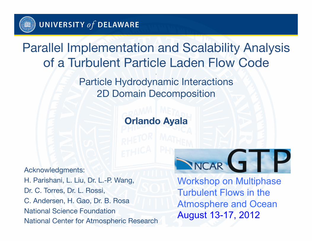
MOTIVATION

1

How does air turbulence affect the collision rates

of cloud droplets?

MOTIVATION

2

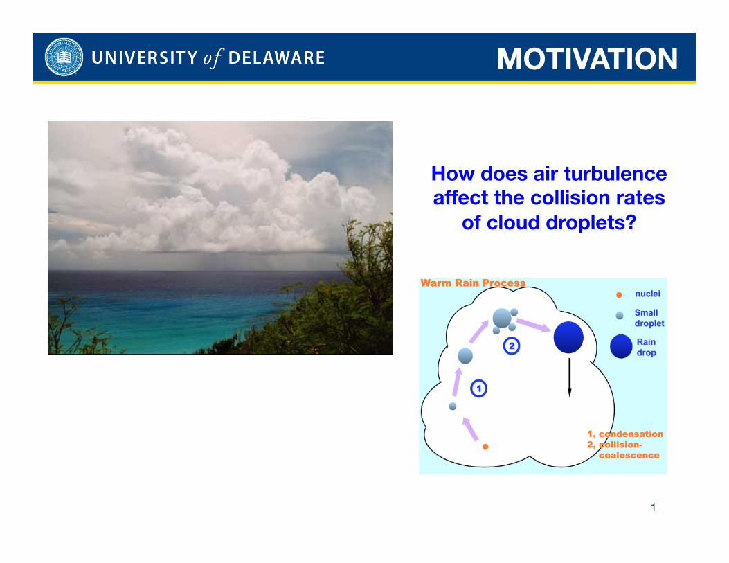
Resolve ~5 orders of magnitude in length

scales

100 to 1000 mm

Δx ~ 1 to 2 mm

a ~ 0.02 to 0.05 mm

Resolved numerically

Treated analytically

MOTIVATION

3

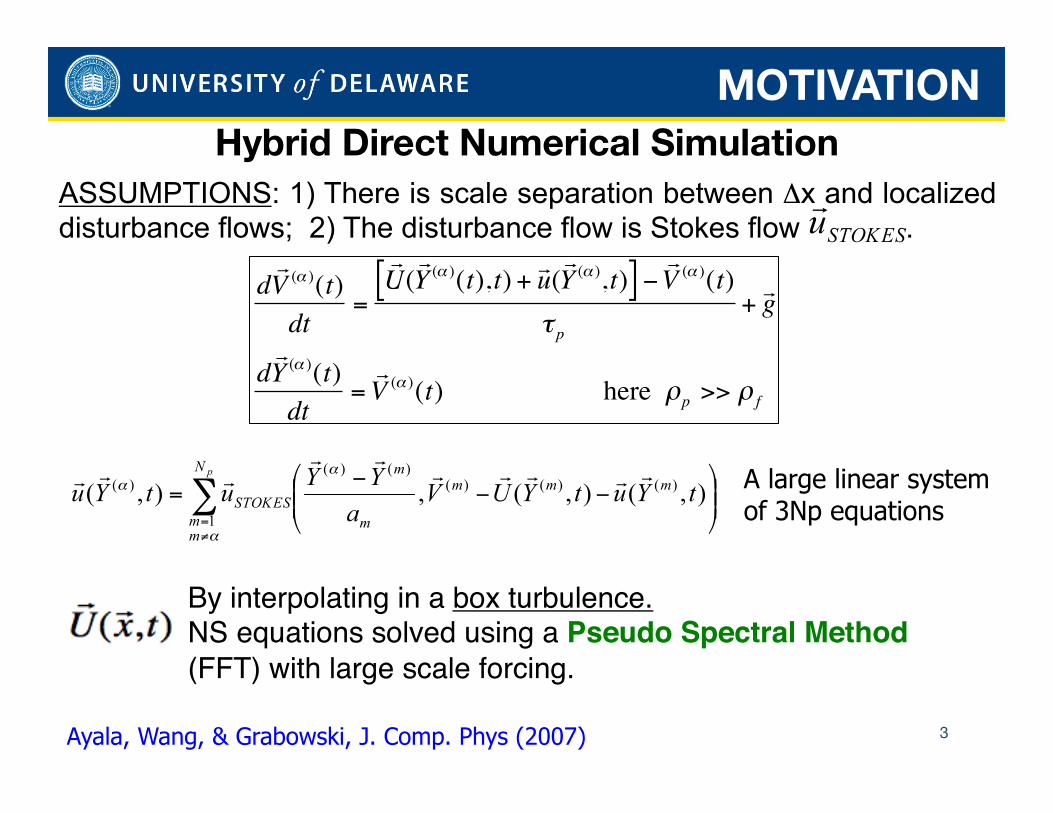
Hybrid Direct Numerical Simulation

€

d V (α )(t)

dt=

U ( Y (α )(t), t) +

u ( Y (α ),t)[ ] −

V (α )(t)

τ p

+ g

d Y (α )(t)

dt=

V (α )(t) here ρp >> ρ f

By interpolating in a box turbulence. !NS equations solved using a Pseudo Spectral Method (FFT) with large scale forcing. !

A large linear system of 3Np equations

ASSUMPTIONS: 1) There is scale separation between Δx and localized disturbance flows; 2) The disturbance flow is Stokes flow .

Ayala, Wang, & Grabowski, J. Comp. Phys (2007)

MOTIVATION

4

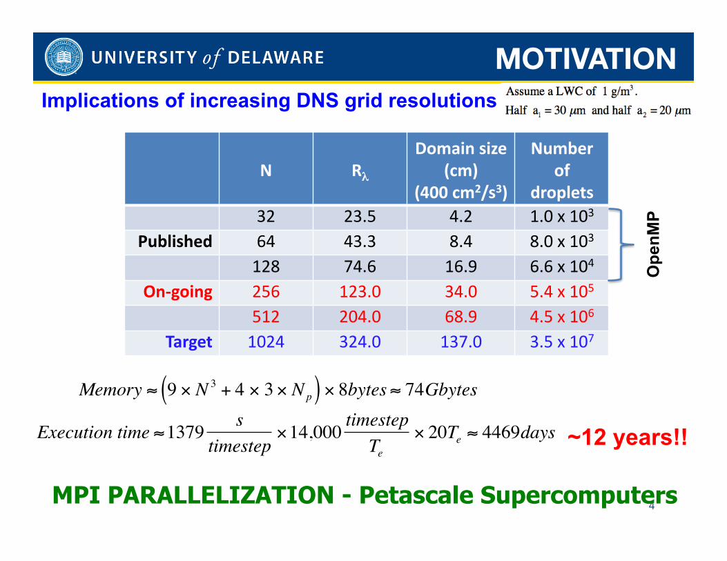
N   Rλ  Domain  size  

(cm)    (400  cm2/s3)  

Number  of  

droplets  32     23.5   4.2   1.0  x  103  

Published   64   43.3   8.4   8.0  x  103  128   74.6   16.9   6.6  x  104  

On-­‐going   256   123.0   34.0   5.4  x  105  512   204.0   68.9   4.5  x  106  

Target   1024   324.0   137.0   3.5  x  107  

MPI PARALLELIZATION - Petascale Supercomputers €

Memory ≈ 9 × N 3 + 4 × 3 × Np( ) × 8bytes ≈ 74Gbytes

€

Execution time ≈1379 stimestep

×14,000 timestepTe

× 20Te ≈ 4469days

Implications of increasing DNS grid resolutions

~12 years!!

Ope

nMP

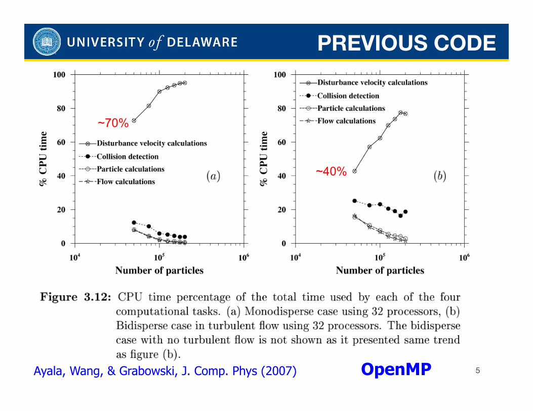
PREVIOUS CODE

5 Ayala, Wang, & Grabowski, J. Comp. Phys (2007) OpenMP

~70%

~40%

Current Research

6

NSF OCI-0904534 Collaborative Research: PetaApps

Enabling Multiscale Modeling of Turbulent Clouds on Petascale

Computers

TO BRIDGE THE GAP BETWEEN LES AND DNS

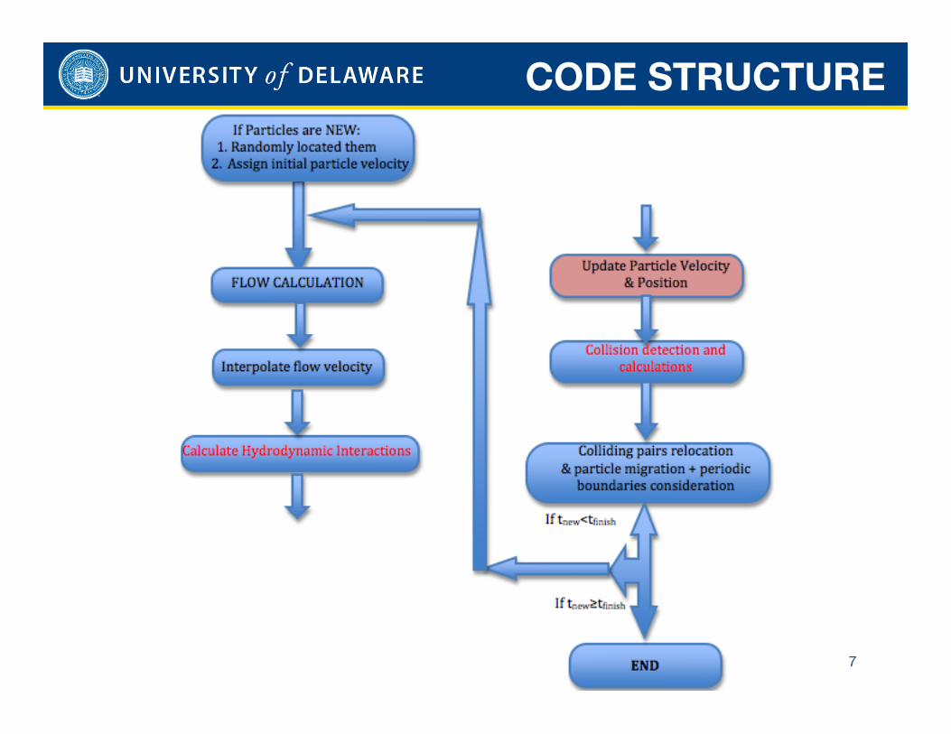
CODE STRUCTURE

7

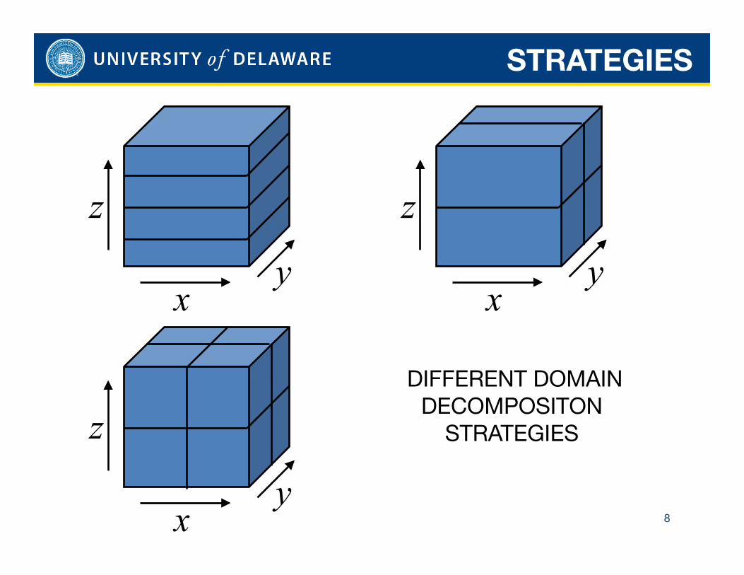
DIFFERENT DOMAIN DECOMPOSITON

STRATEGIES

8

STRATEGIES

9

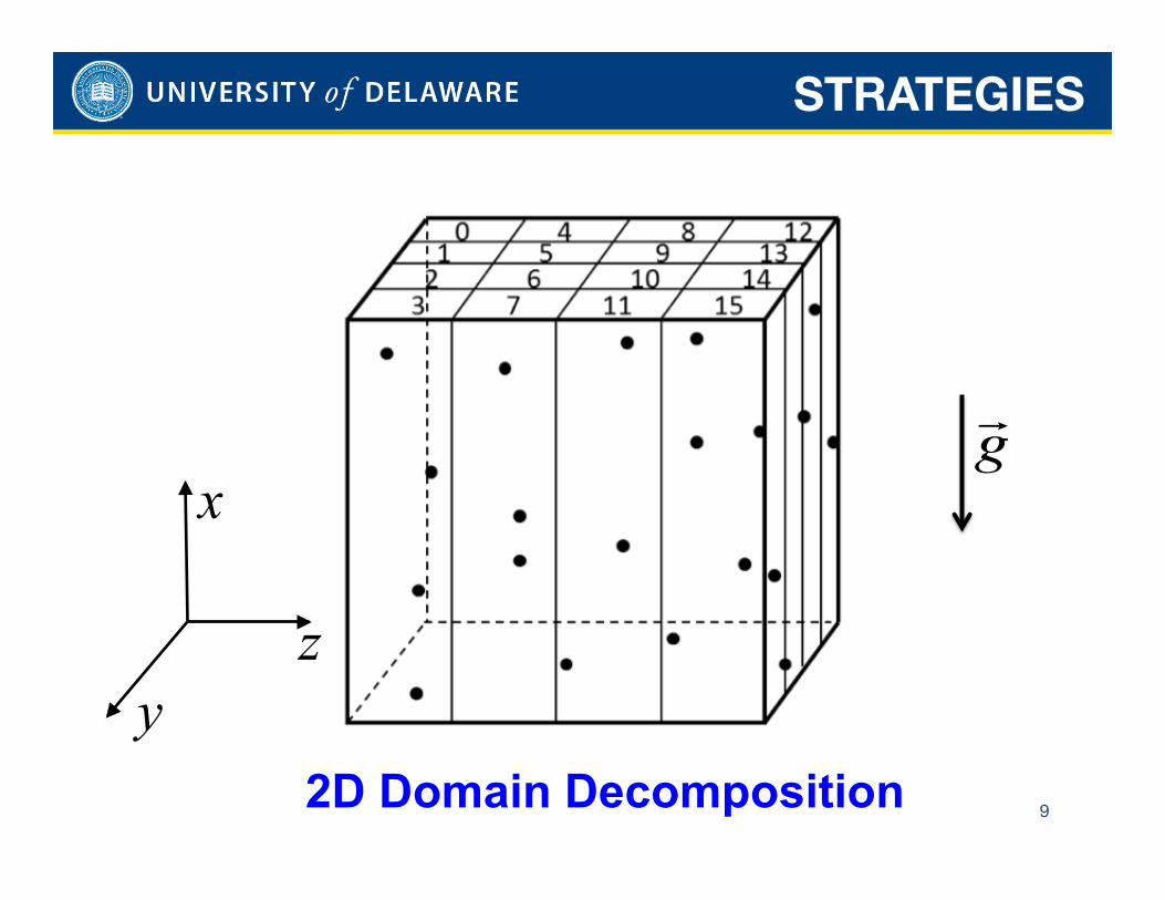
STRATEGIES

€

g

2D Domain Decomposition

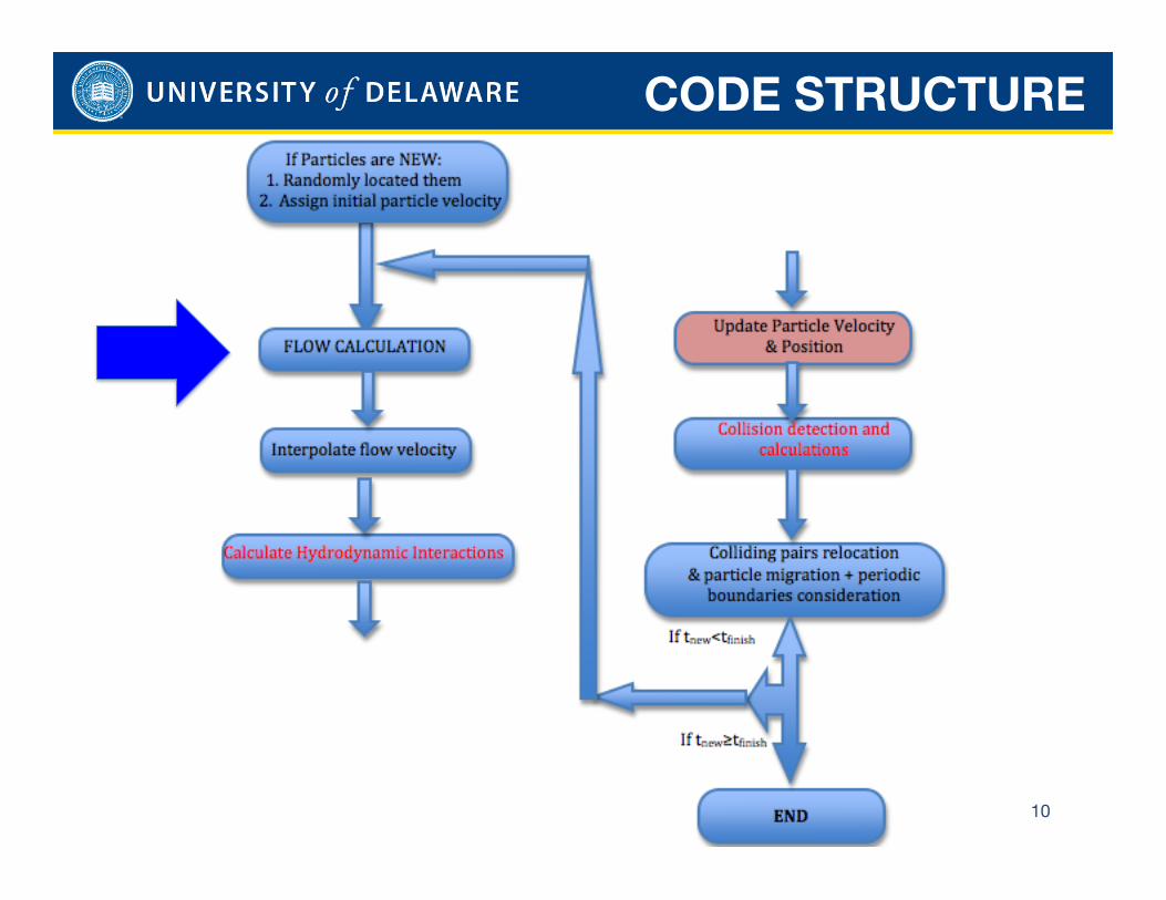
CODE STRUCTURE

10

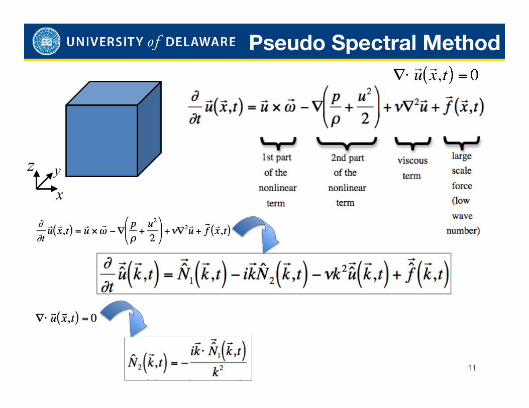
Pseudo Spectral Method

11

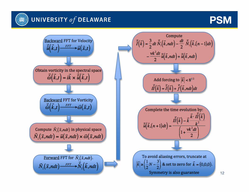
PSM

12

PSM

13

14

PSM

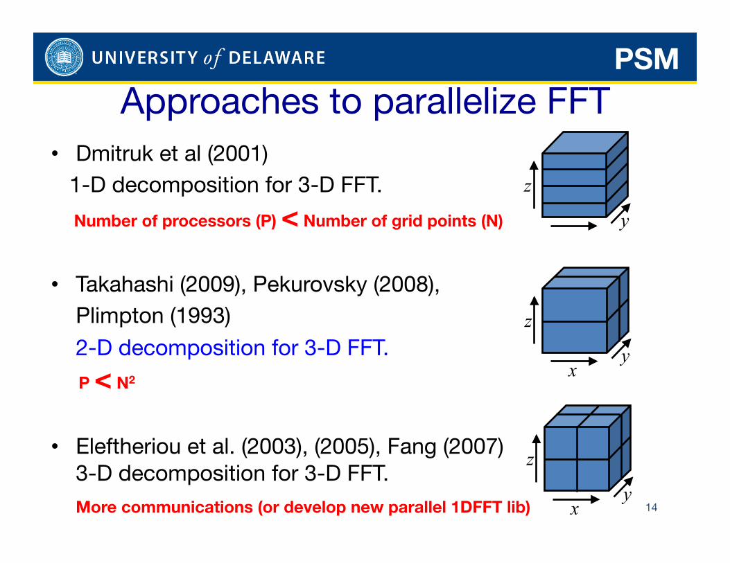
Approaches to parallelize FFT •  Dmitruk et al (2001) 1-D decomposition for 3-D FFT.

Number of processors (P) < Number of grid points (N)

•  Takahashi (2009), Pekurovsky (2008), Plimpton (1993)

2-D decomposition for 3-D FFT.

P < N2

•  Eleftheriou et al. (2003), (2005), Fang (2007)!3-D decomposition for 3-D FFT.

More communications (or develop new parallel 1DFFT lib)

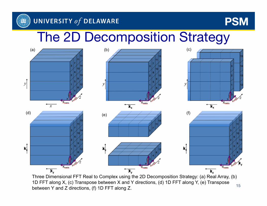
The 2D Decomposition Strategy

15

(a) (b)

(d) (e) (f)

Three Dimensional FFT Real to Complex using the 2D Decomposition Strategy: (a) Real Array, (b) 1D FFT along X, (c) Transpose between X and Y directions, (d) 1D FFT along Y, (e) Transpose between Y and Z directions, (f) 1D FFT along Z.

(c)

PSM

kx kx

kx kx

ky ky

kx

ky

kz

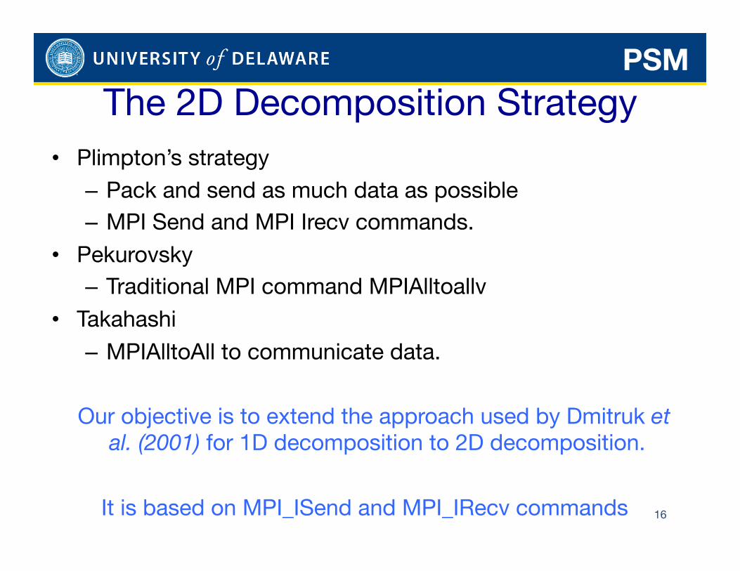
The 2D Decomposition Strategy •  Plimpton’s strategy

–  Pack and send as much data as possible –  MPI Send and MPI Irecv commands.

•  Pekurovsky –  Traditional MPI command MPIAlltoallv

•  Takahashi

–  MPIAlltoAll to communicate data.

Our objective is to extend the approach used by Dmitruk et al. (2001) for 1D decomposition to 2D decomposition.

It is based on MPI_ISend and MPI_IRecv commands 16

PSM

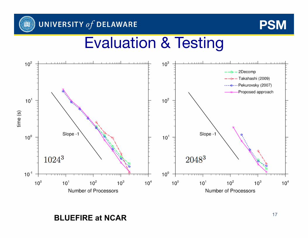
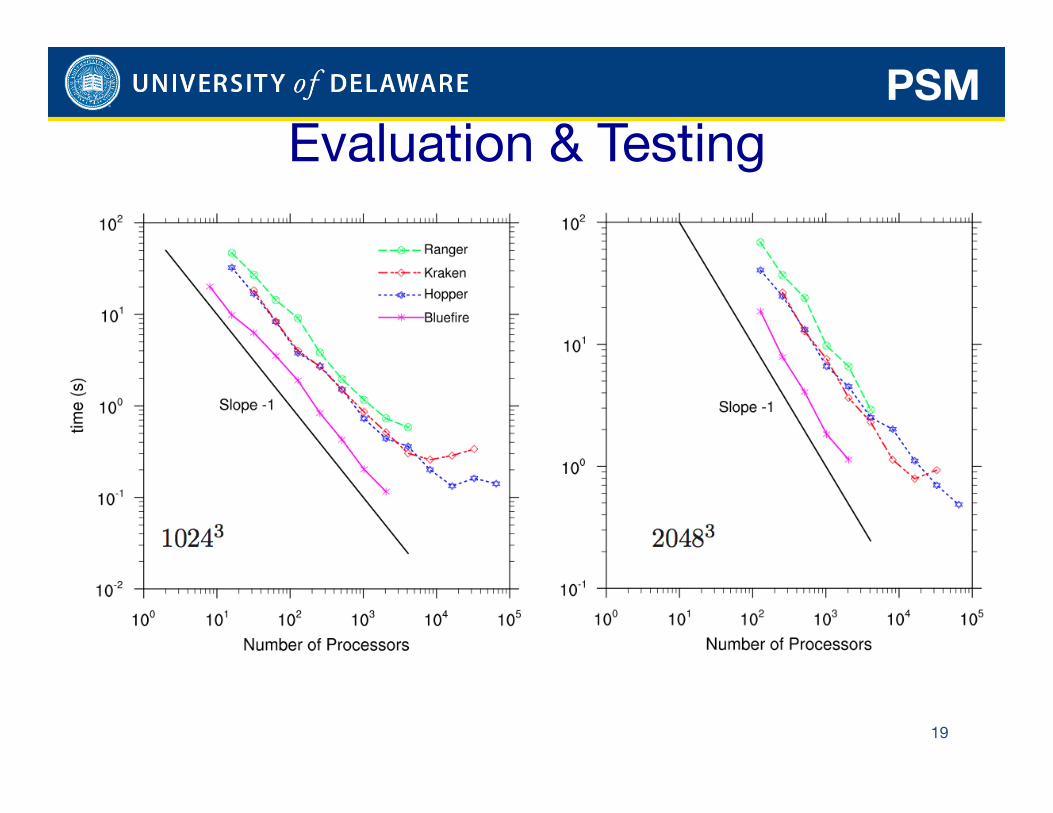
Evaluation & Testing

17 BLUEFIRE at NCAR

PSM

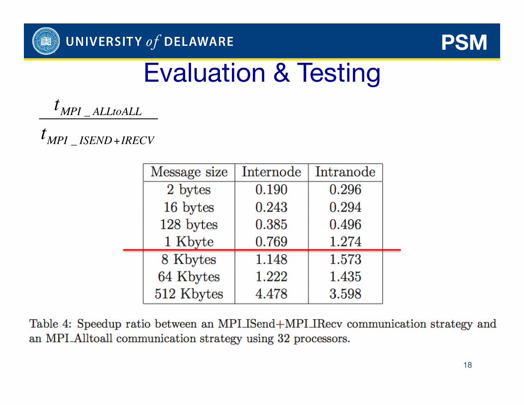
Evaluation & Testing

18

PSM

€

tMPI _ ALLtoALLtMPI _ ISEND+IRECV

19

Evaluation & Testing PSM

20

€

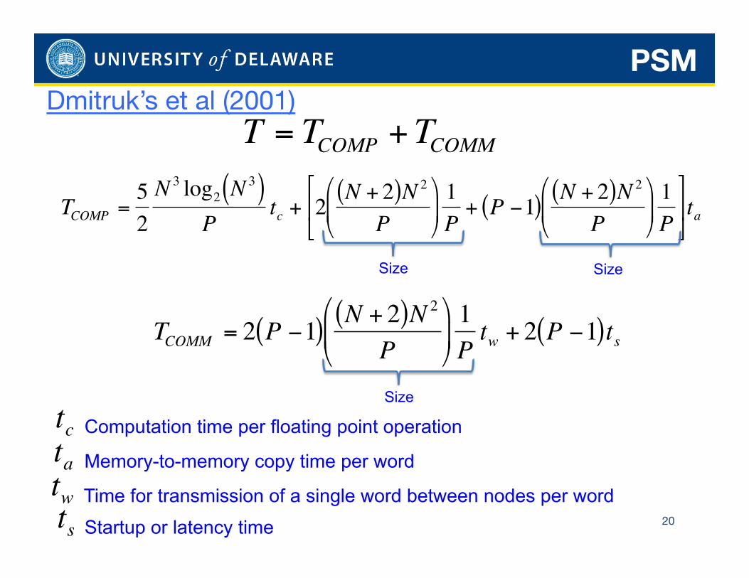
T = TCOMP +TCOMM

€

TCOMP =52N 3 log2 N

3( )P

tc + 2 N + 2( )N 2

P⎛

⎝ ⎜

⎞

⎠ ⎟ 1P

+ P −1( ) N + 2( )N 2

P⎛

⎝ ⎜

⎞

⎠ ⎟ 1P

⎡

⎣ ⎢

⎤

⎦ ⎥ ta

€

TCOMM = 2 P −1( ) N + 2( )N 2

P⎛

⎝ ⎜

⎞

⎠ ⎟ 1Ptw + 2 P −1( )ts

€

tc Computation time per floating point operation

Memory-to-memory copy time per word

€

taTime for transmission of a single word between nodes per word

€

twStartup or latency time

€

ts

Size Size

Size

Dmitruk’s et al (2001) PSM

21

€

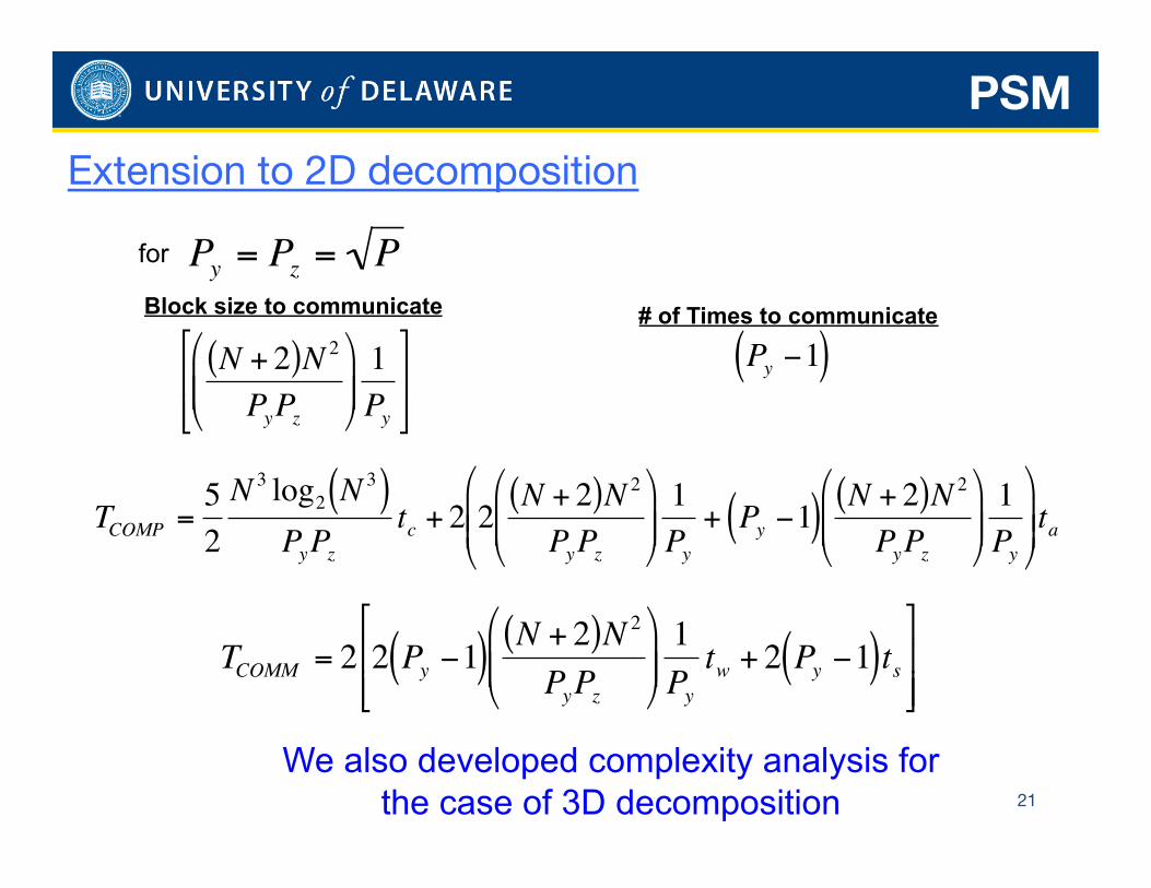
TCOMP =52N 3 log2 N

3( )PyPz

tc + 2 2 N + 2( )N 2

PyPz

⎛

⎝ ⎜ ⎜

⎞

⎠ ⎟ ⎟ 1Py

+ Py −1( ) N + 2( )N 2

PyPz

⎛

⎝ ⎜ ⎜

⎞

⎠ ⎟ ⎟ 1Py

⎛

⎝ ⎜ ⎜

⎞

⎠ ⎟ ⎟ ta

€

TCOMM = 2 2 Py −1( ) N + 2( )N 2

PyPz

⎛

⎝ ⎜ ⎜

⎞

⎠ ⎟ ⎟ 1Pytw + 2 Py −1( )ts

⎡

⎣ ⎢ ⎢

⎤

⎦ ⎥ ⎥

for

€

Py = Pz = P

€

N + 2( )N 2

PyPz

⎛

⎝ ⎜ ⎜

⎞

⎠ ⎟ ⎟ 1Py

⎡

⎣ ⎢ ⎢

⎤

⎦ ⎥ ⎥

Block size to communicate

€

Py −1( )# of Times to communicate

Extension to 2D decomposition

PSM

We also developed complexity analysis for the case of 3D decomposition

22

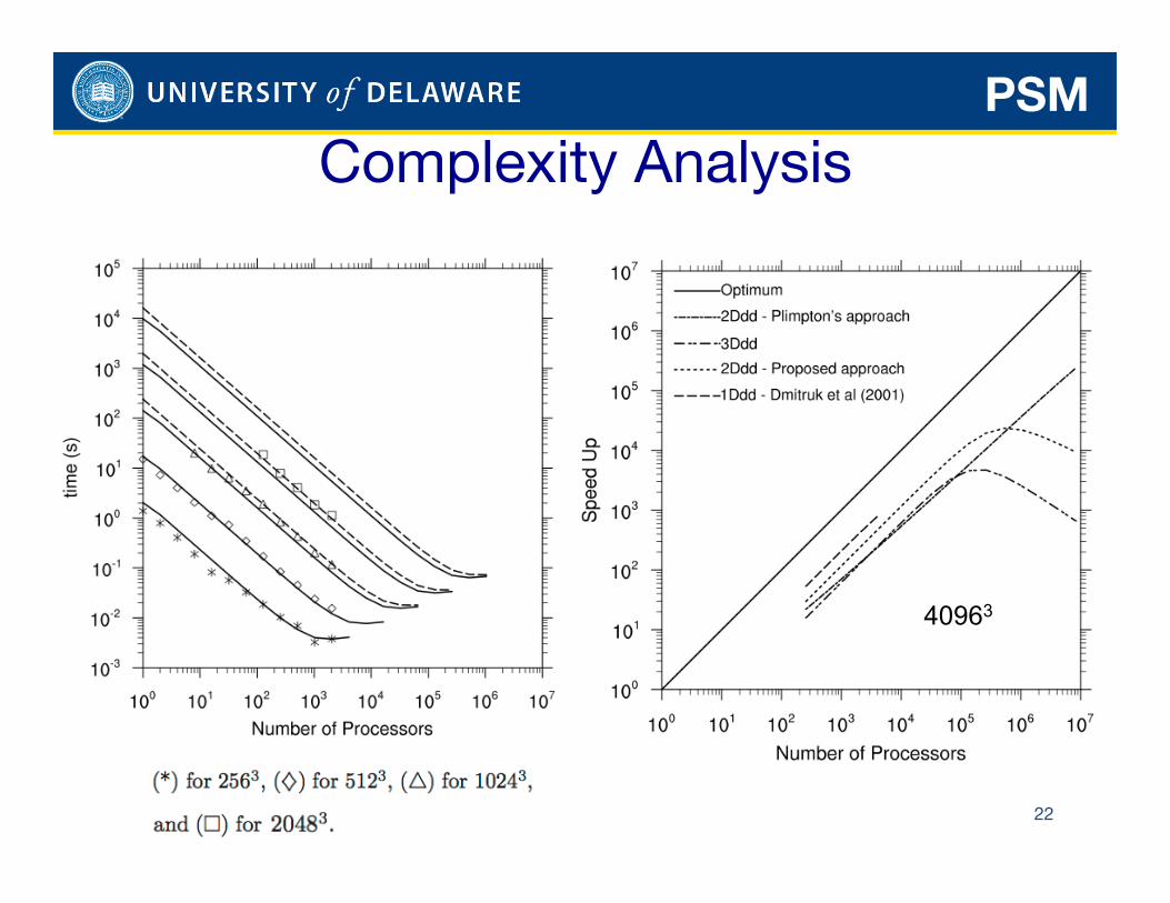
Complexity Analysis PSM

40963

PSM

23

0.01  

0.1  

1  

10  

1   10   100   1000   10000  

Cme  (s)  

Number  of  Processors  

512^3  Data  

512^3  Theory  

1024^3  Data  

1024^3  Theory  

€

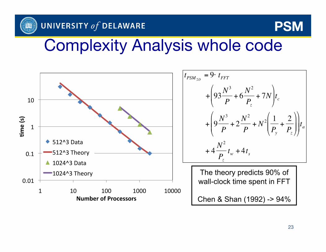
tPSM 2D= 9⋅ tFFT

+ 93N3

P+ 6 N

2

Pz+ 7N

⎛

⎝ ⎜

⎞

⎠ ⎟ tc

+ 9 N3

P+ 2 N

2

P+ N 2 1

Py+

2Pz

⎛

⎝ ⎜ ⎜

⎞

⎠ ⎟ ⎟

⎛

⎝ ⎜ ⎜

⎞

⎠ ⎟ ⎟ ta

+ 4 N2

Pztw + 4ts

Complexity Analysis whole code

The theory predicts 90% of wall-clock time spent in FFT

Chen & Shan (1992) -> 94%

PSM

24

What about LBM or FDM?

LBM

25

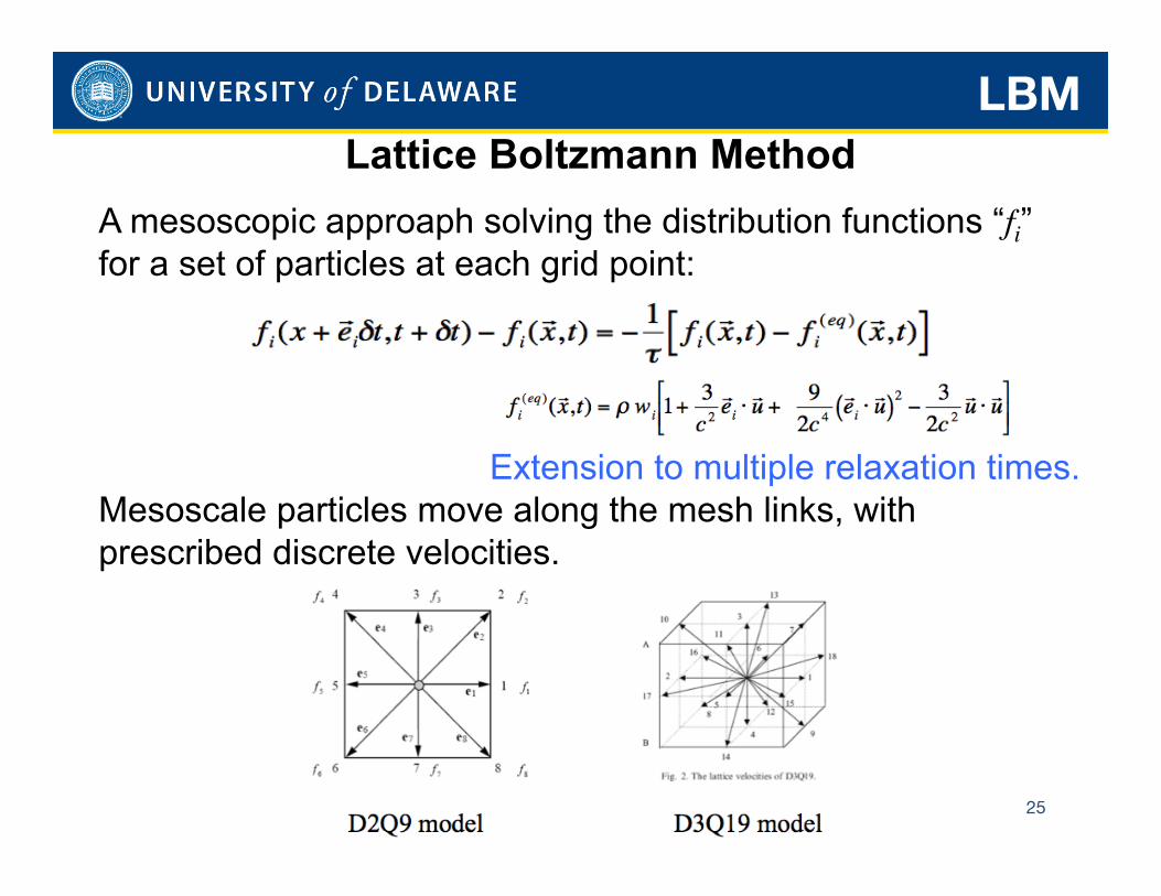
Lattice Boltzmann Method A mesoscopic approaph solving the distribution functions “fi” for a set of particles at each grid point:

Extension to multiple relaxation times. Mesoscale particles move along the mesh links, with prescribed discrete velocities.

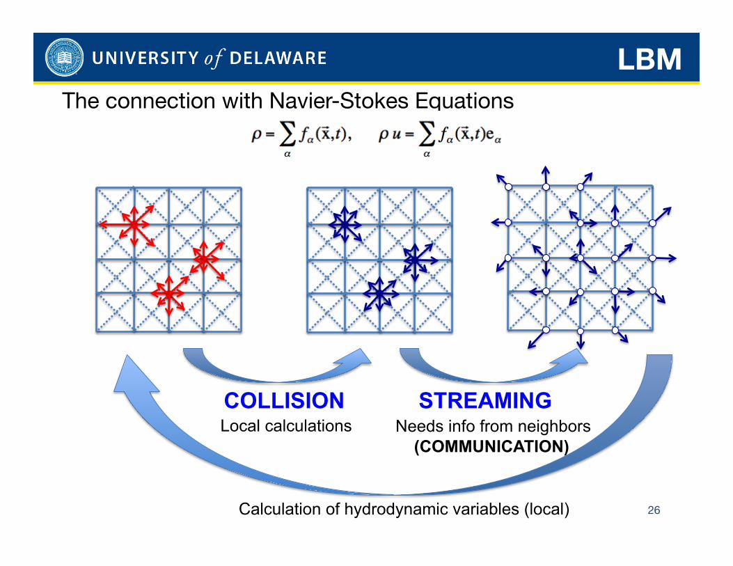
LBM The connection with Navier-Stokes Equations

26

COLLISION STREAMING Local calculations Needs info from neighbors

(COMMUNICATION)

Calculation of hydrodynamic variables (local)

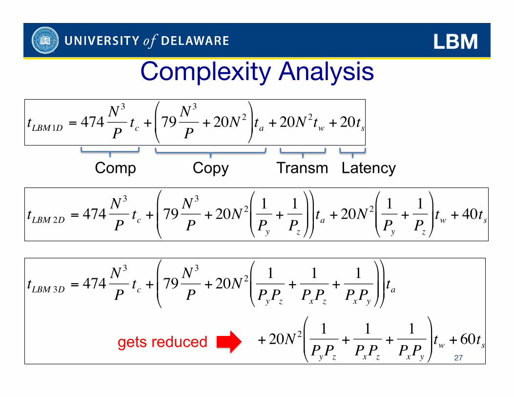
LBM

27

Comp Copy Transm Latency

€

tLBM 1D = 474 N3

Ptc + 79 N

3

P+ 20N 2

⎛

⎝ ⎜

⎞

⎠ ⎟ ta + 20N 2tw + 20ts

€

tLBM 2D = 474 N3

Ptc + 79 N

3

P+ 20N 2 1

Py+1Pz

⎛

⎝ ⎜ ⎜

⎞

⎠ ⎟ ⎟

⎛

⎝ ⎜ ⎜

⎞

⎠ ⎟ ⎟ ta + 20N 2 1

Py+1Pz

⎛

⎝ ⎜ ⎜

⎞

⎠ ⎟ ⎟ tw + 40ts

€

tLBM 3D = 474 N3

Ptc + 79 N

3

P+ 20N 2 1

PyPz+

1PxPz

+1PxPy

⎛

⎝ ⎜ ⎜

⎞

⎠ ⎟ ⎟

⎛

⎝ ⎜ ⎜

⎞

⎠ ⎟ ⎟ ta

+ 20N 2 1PyPz

+1PxPz

+1PxPy

⎛

⎝ ⎜ ⎜

⎞

⎠ ⎟ ⎟ tw + 60ts

Complexity Analysis

gets reduced

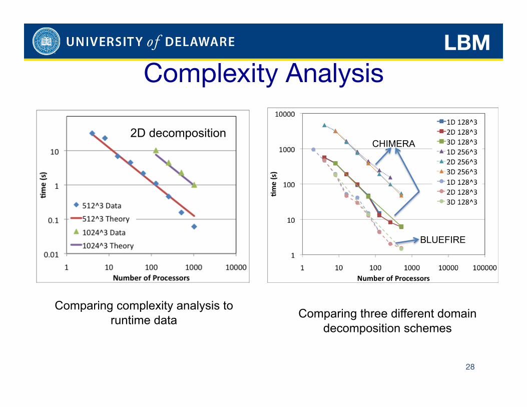
LBM

28

2D decomposition

Comparing complexity analysis to runtime data Comparing three different domain

decomposition schemes

CHIMERA

BLUEFIRE

Complexity Analysis

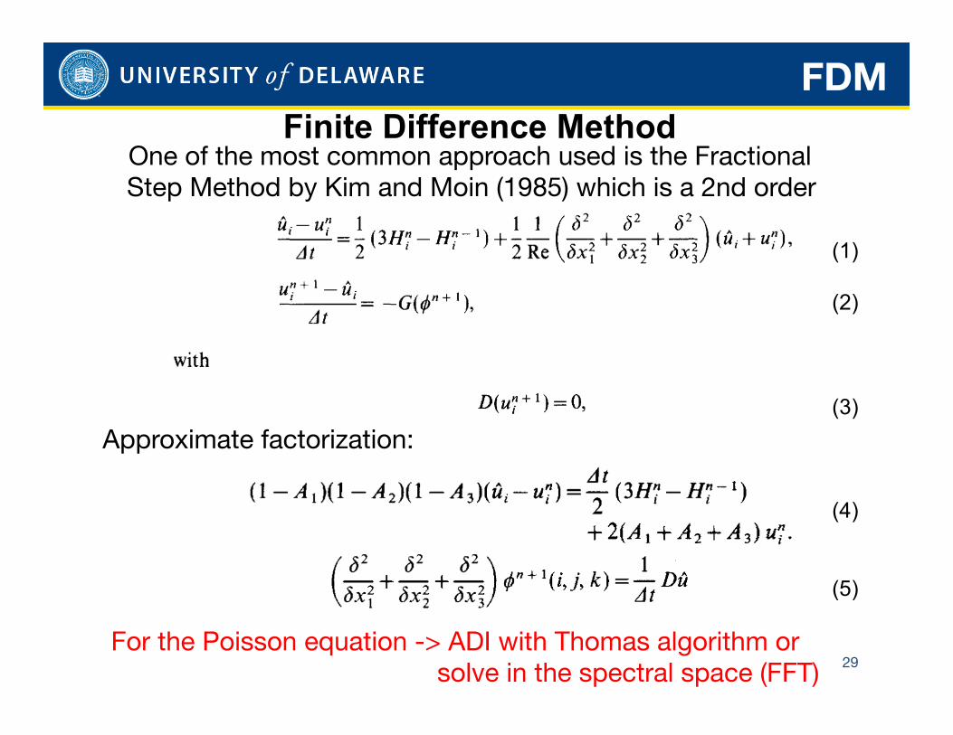
FDM

One of the most common approach used is the Fractional Step Method by Kim and Moin (1985) which is a 2nd order

method

29

Finite Difference Method

Approximate factorization:

(1)

(2)

(3)

(4)

(5)

For the Poisson equation -> ADI with Thomas algorithm or solve in the spectral space (FFT)

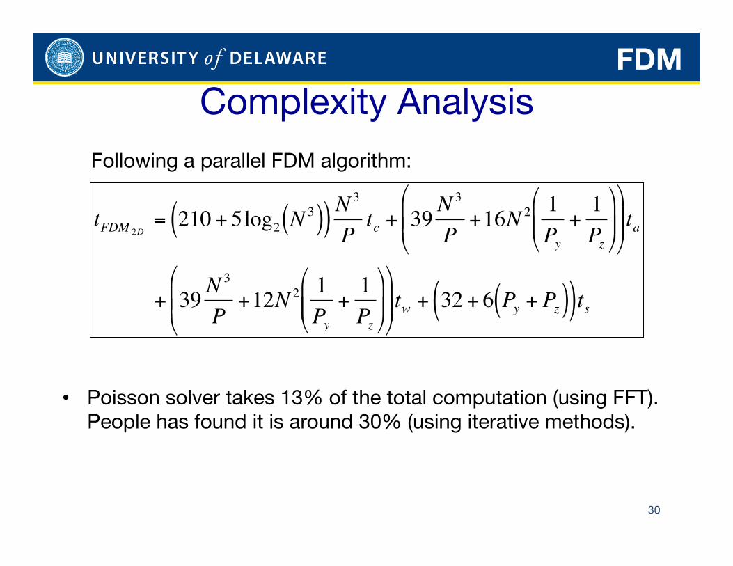
FDM

30

Complexity Analysis

€

tFDM 2D= 210 + 5log2 N

3( )( ) N3

Ptc + 39 N

3

P+16N 2 1

Py+

1Pz

⎛

⎝ ⎜ ⎜

⎞

⎠ ⎟ ⎟

⎛

⎝ ⎜ ⎜

⎞

⎠ ⎟ ⎟ ta

+ 39 N3

P+12N 2 1

Py+

1Pz

⎛

⎝ ⎜ ⎜

⎞

⎠ ⎟ ⎟

⎛

⎝ ⎜ ⎜

⎞

⎠ ⎟ ⎟ tw + 32 + 6 Py + Pz( )( )ts

•  Poisson solver takes 13% of the total computation (using FFT). People has found it is around 30% (using iterative methods).

Following a parallel FDM algorithm:

FLOW COMPARISON

31

2563

2563

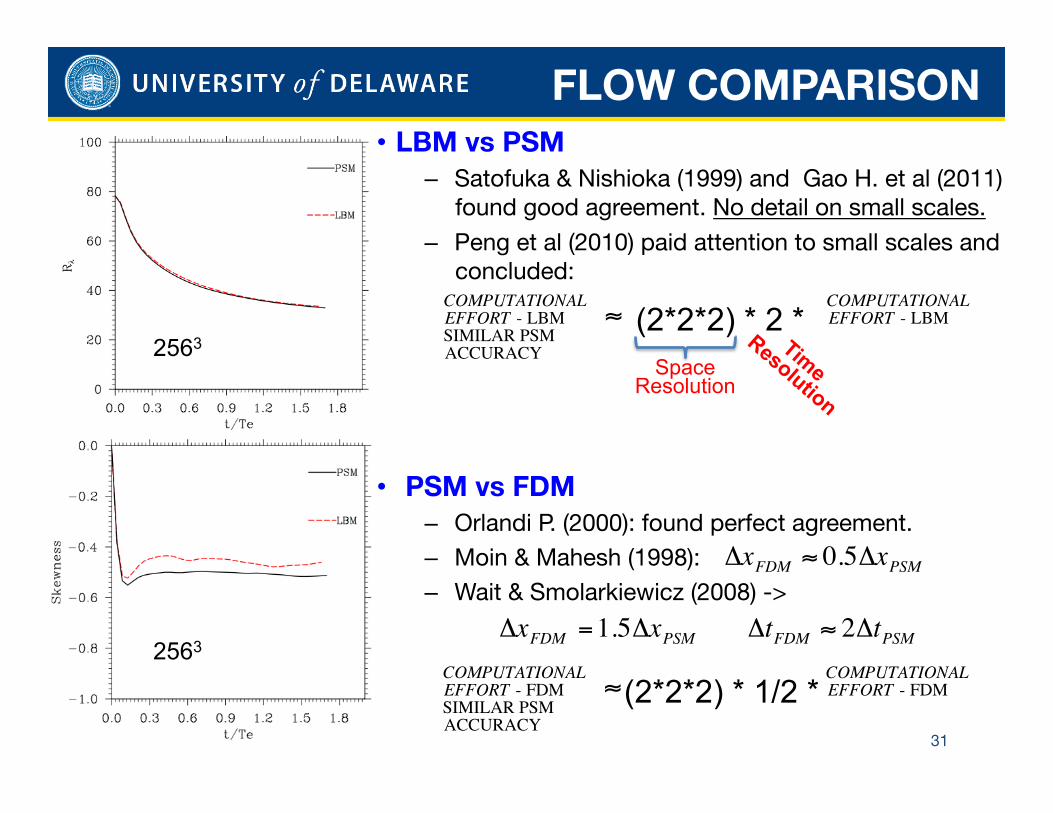
•  LBM vs PSM –  Satofuka & Nishioka (1999) and Gao H. et al (2011)

found good agreement. No detail on small scales.

–  Peng et al (2010) paid attention to small scales and concluded:

•  PSM vs FDM –  Orlandi P. (2000): found perfect agreement. –  Moin & Mahesh (1998): –  Wait & Smolarkiewicz (2008) ->

€

ΔxFDM ≈ 0.5ΔxPSM

€

ΔxFDM =1.5ΔxPSM ΔtFDM ≈ 2ΔtPSM

€

COMPUTATIONAL COMPUTATIONALEFFORT - LBM ≈ EFFORT - LBMSIMILAR PSMACCURACY

(2*2*2) * 2 *

(2*2*2) * 1/2 *

Space Resolution

€

COMPUTATIONAL COMPUTATIONALEFFORT - FDM ≈ EFFORT - FDMSIMILAR PSMACCURACY

32

0.001  0.01  0.1  1  

10  100  1000  

10000  100000  

1000000  10000000  100000000  

1.E+00   1.E+01   1.E+02   1.E+03   1.E+04   1.E+05  

Pred

icted  Co

mpu

taCon

al  Cme  (s)  

Problem  Size  

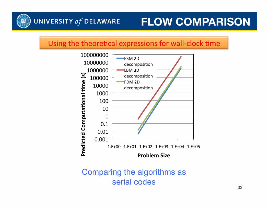
PSM  2D  decomposiCon  LBM  3D  decomposiCon  FDM  2D  decomposiCon  

Comparing the algorithms as serial codes

Using  the  theoreCcal  expressions  for  wall-­‐clock  Cme  

FLOW COMPARISON

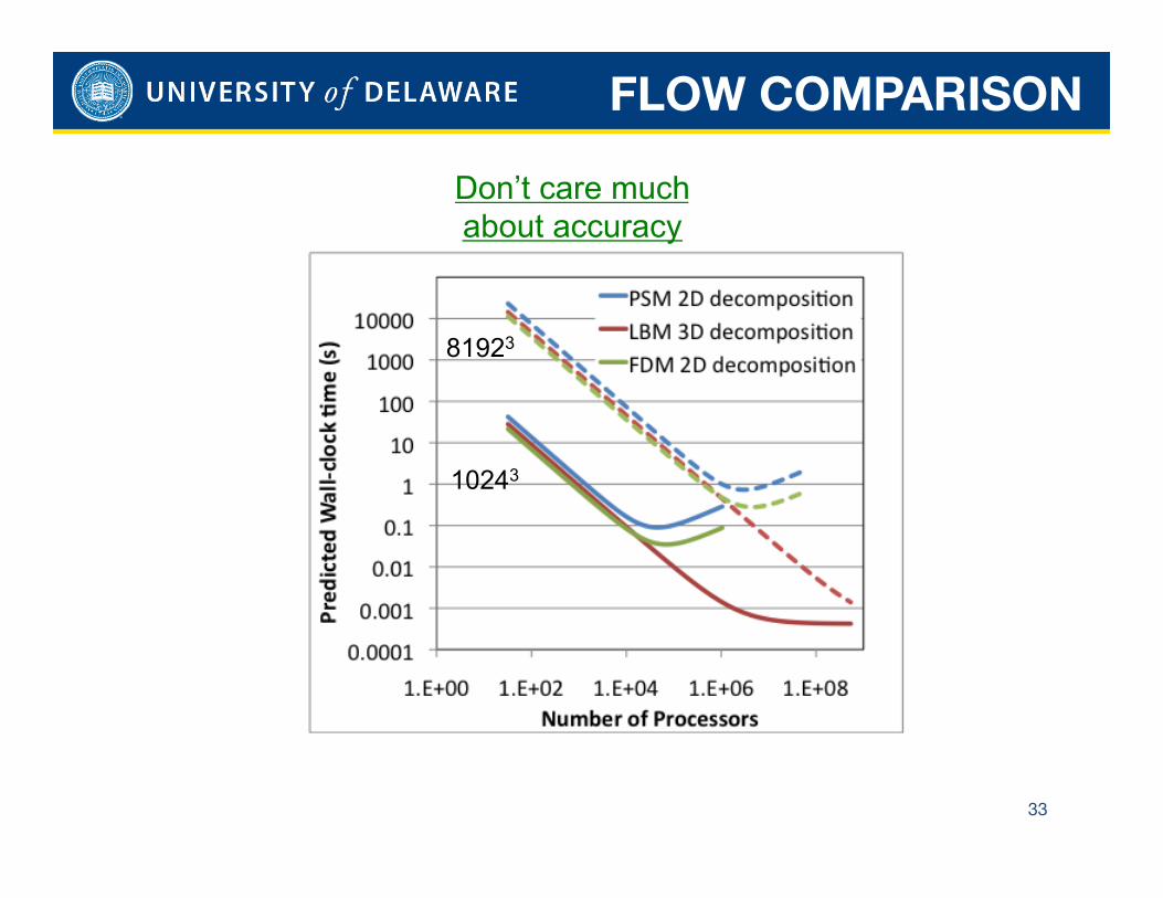
33

10243

81923

FLOW COMPARISON

Don’t care much about accuracy

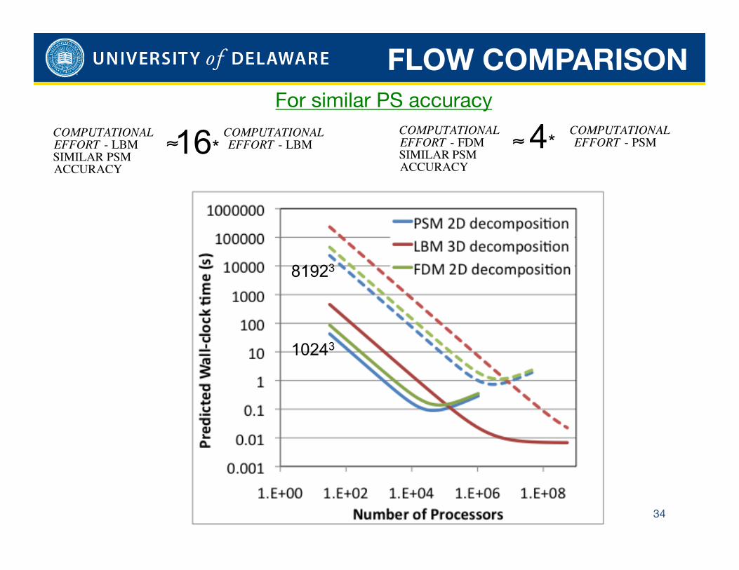
For similar PS accuracy

34

10243

81923 €

COMPUTATIONAL COMPUTATIONALEFFORT - LBM ≈ EFFORT - LBMSIMILAR PSMACCURACY

16*

€

COMPUTATIONAL COMPUTATIONALEFFORT - FDM ≈ EFFORT - PSMSIMILAR PSMACCURACY

4*

FLOW COMPARISON

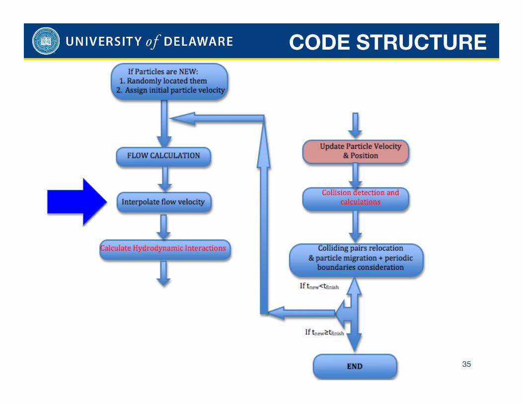
CODE STRUCTURE

35

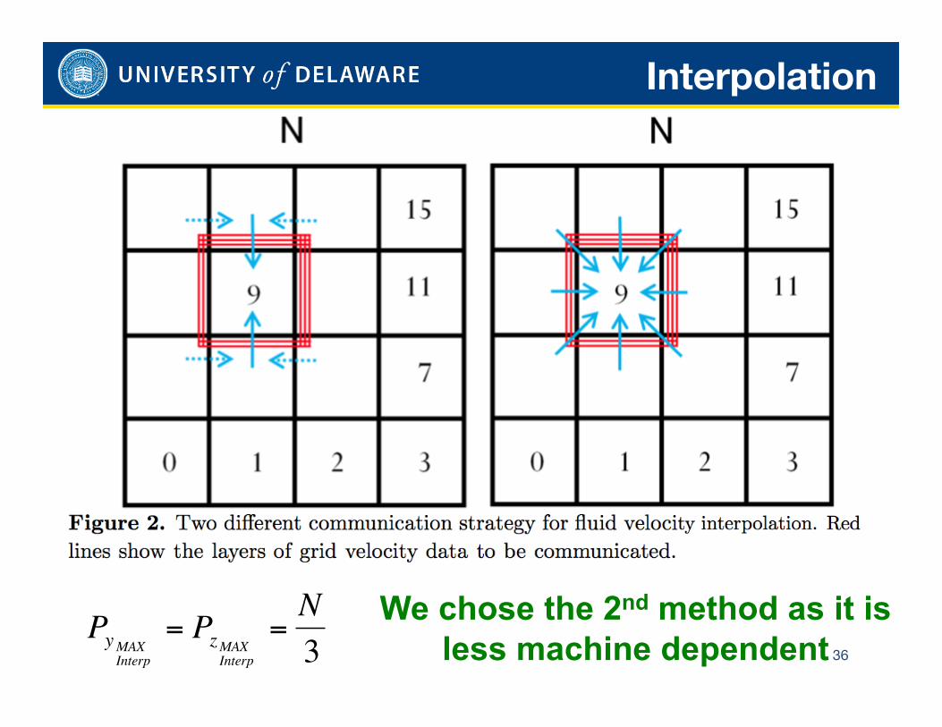
Interpolation

36

We chose the 2nd method as it is less machine dependent

€

PyMAXInterp

= PzMAXInterp

=N3

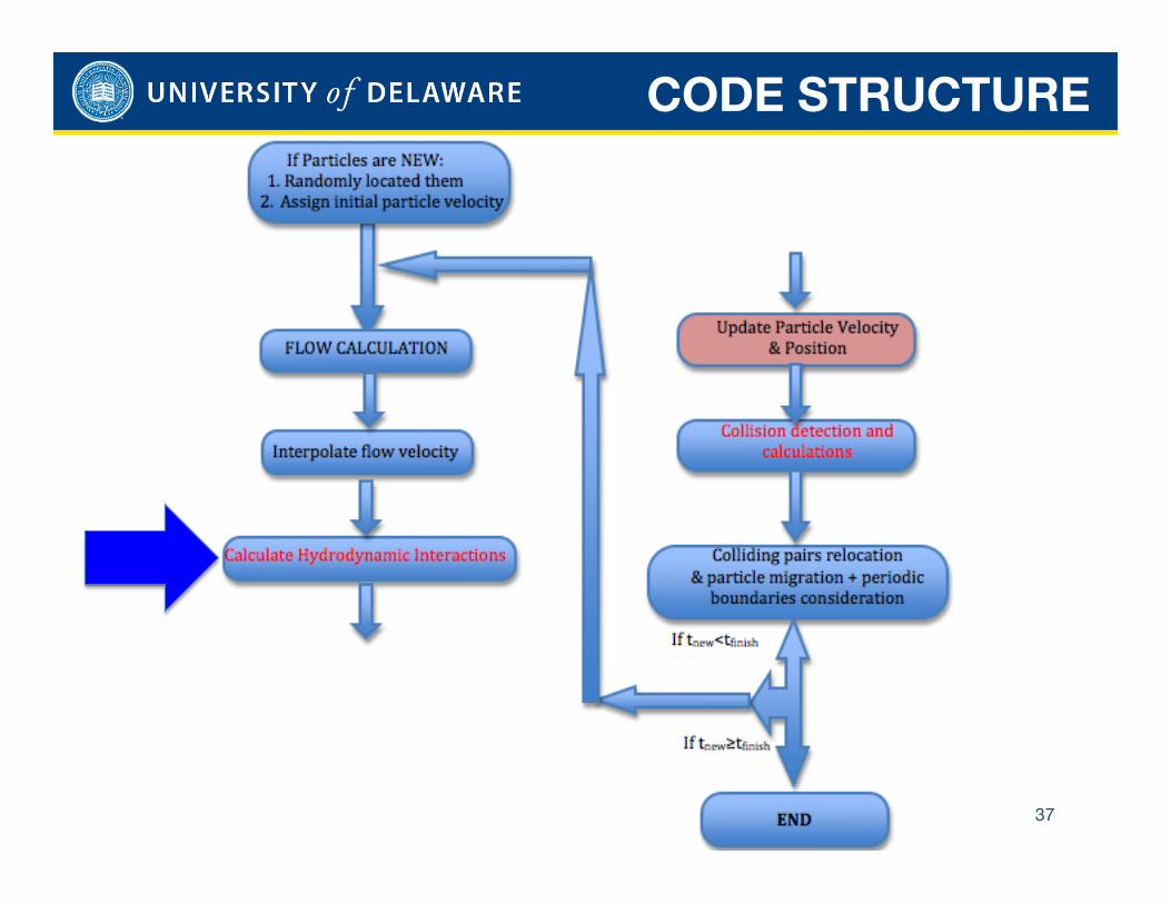
CODE STRUCTURE

37

HDI

38

Preprint submitted to J. Computational Physics April 19, 2012

HDI

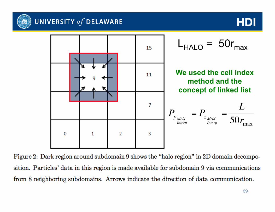
39

LHALO = 50rmax

We used the cell index method and the

concept of linked list

€

PyMAXInterp

= PzMAXInterp

=L

50rmax

HDI

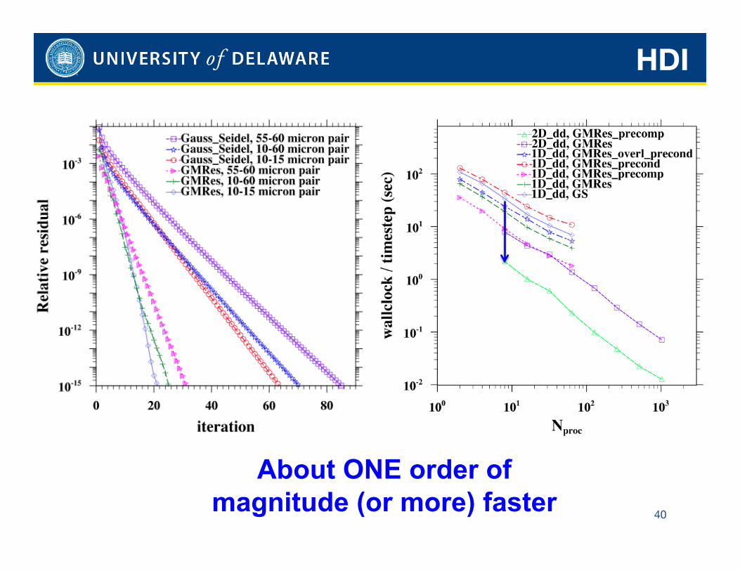
40

About ONE order of magnitude (or more) faster

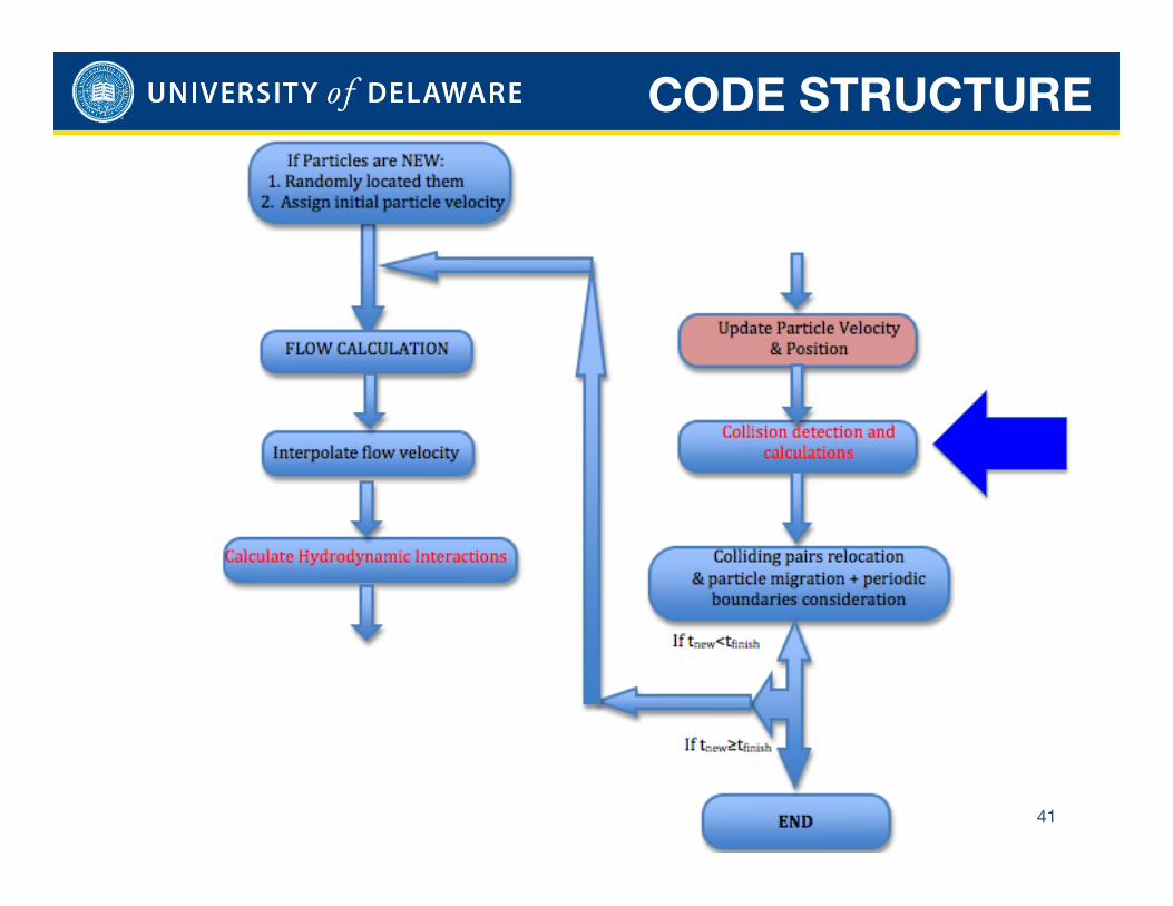
CODE STRUCTURE

41

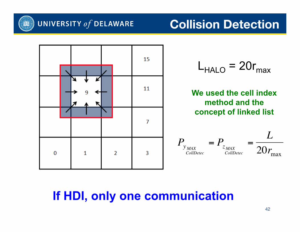
Collision Detection

42

LHALO = 20rmax

If HDI, only one communication

We used the cell index method and the

concept of linked list

€

PyMAXCollDetec

= PzMAXCollDetec

=L

20rmax

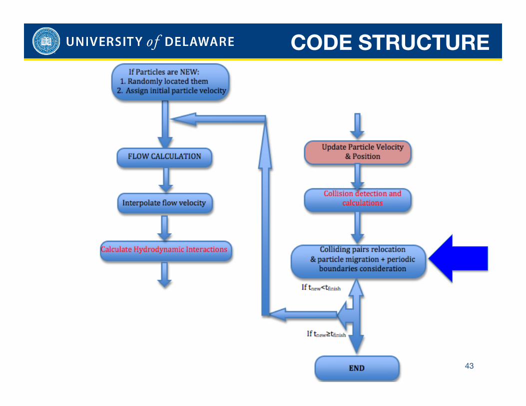
CODE STRUCTURE

43

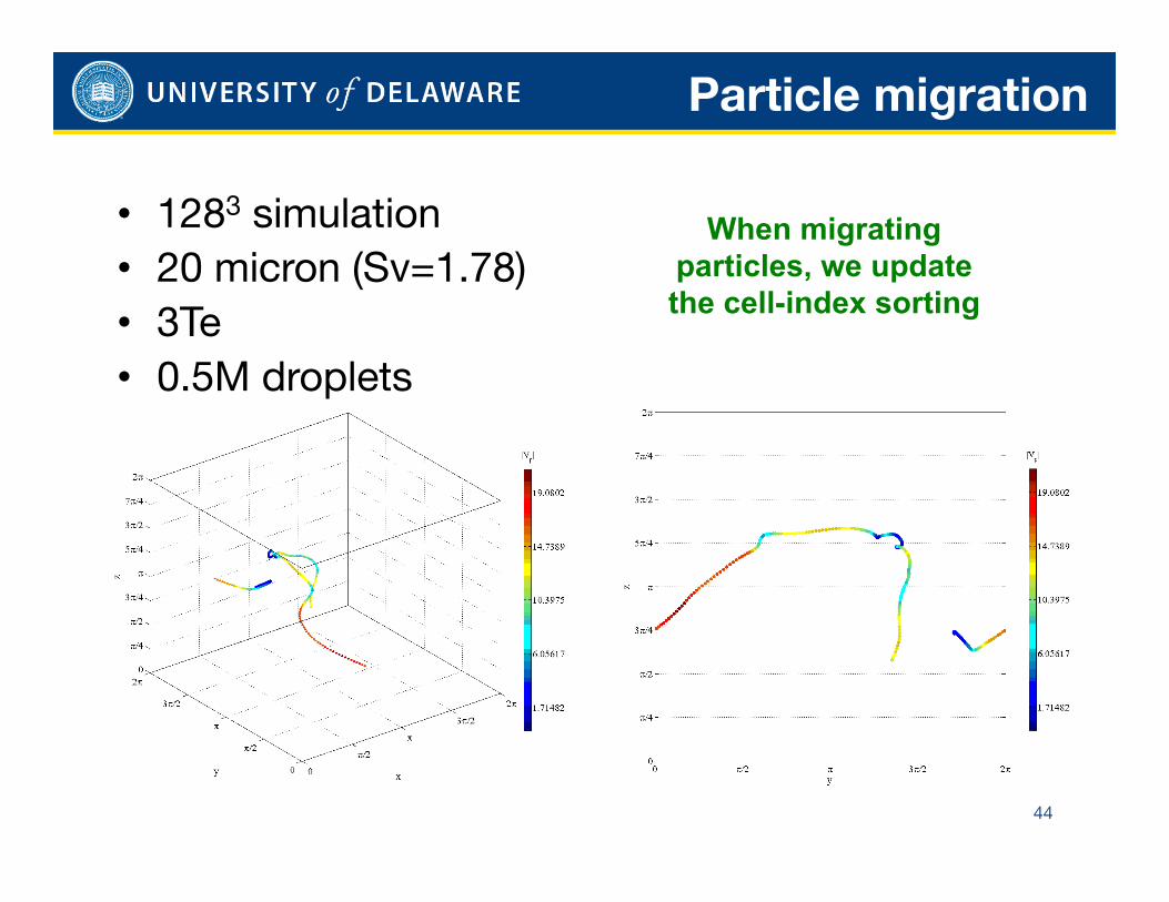
Particle migration

44

•  1283 simulation •  20 micron (Sv=1.78) •  3Te •  0.5M droplets

When migrating particles, we update the cell-index sorting

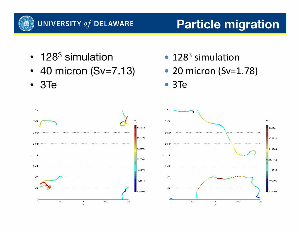
Particle migration

45

•  1283 simulation •  40 micron (Sv=7.13) •  3Te

  1283  simulaCon    20  micron  (Sv=1.78)    3Te  

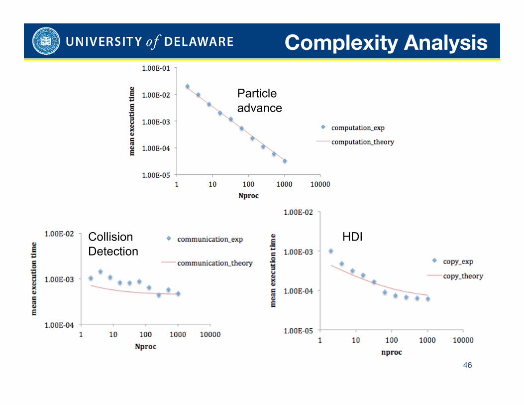
Complexity Analysis

46

Particle advance

Collision Detection

HDI

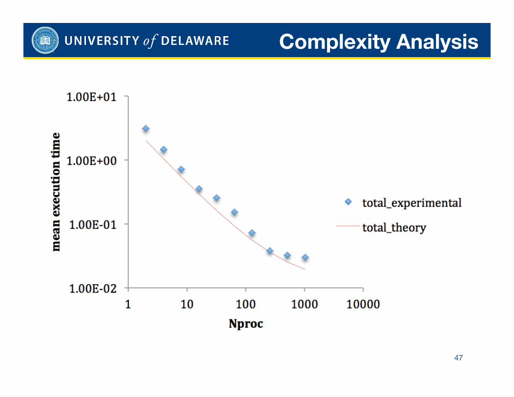
Complexity Analysis

47

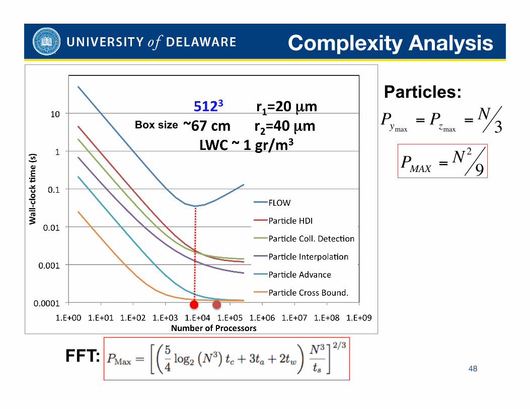
Complexity Analysis

48

€

Pymax = Pzmax = N 3

€

PMAX = N2

9

FFT:

Particles:

Box size

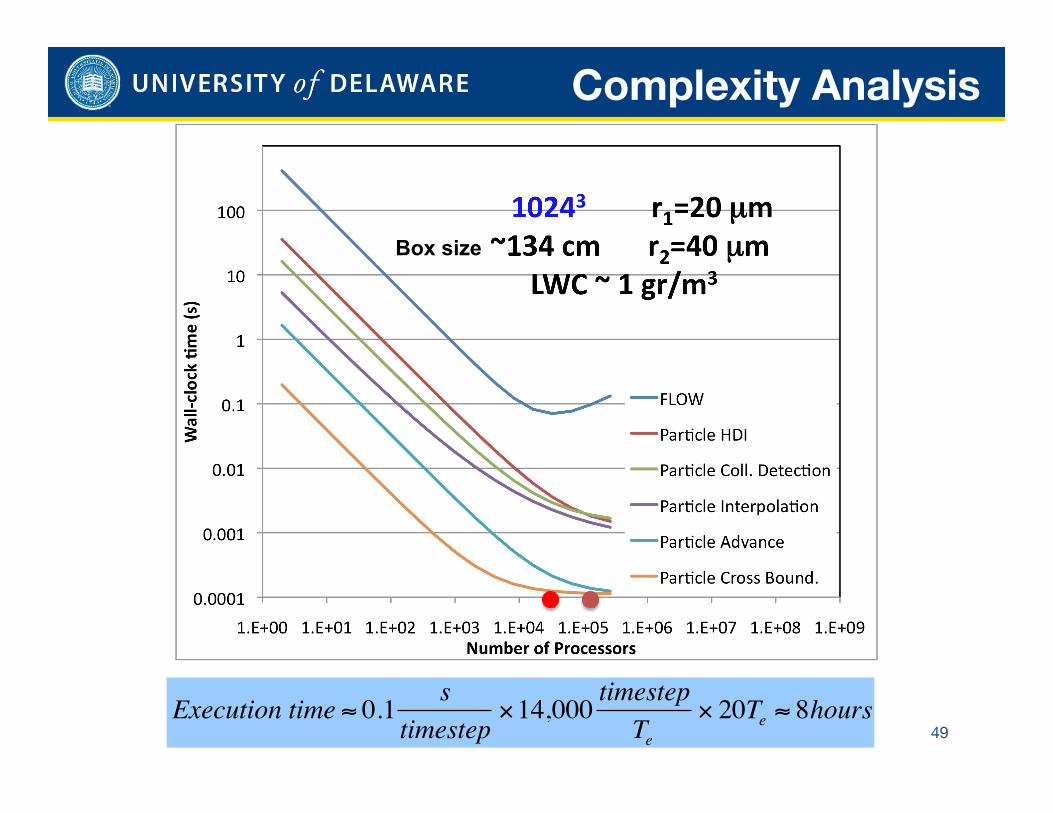
Complexity Analysis

49

€

Execution time ≈ 0.1 stimestep

×14,000 timestepTe

× 20Te ≈ 8hours

Box size

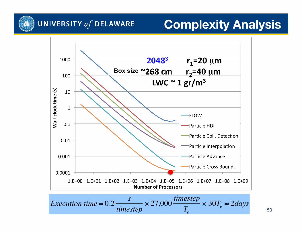
Complexity Analysis

50

€

Execution time ≈ 0.2 stimestep

× 27,000 timestepTe

× 30Te ≈ 2days

Box size

CONCLUSIONS

51

 We have developed a highly scalable parallel code to model homogeneous isotropic turbulence with inertial particles using 2D domain decomposition.

 We were able to optimize HDI calculations. Now the flow (or FFT) calculations are the bottleneck (Pmax).

  In comparison to LBM and FDM, PSM is still a good choice to model HI turbulence in Supercomputers. It is more accurate and, for similar accuracy, it is comparable in terms of parallel performance.

  IMPROVEMENTS • OpenMP+MPI (but if large P, might not help).

• GPU+CPU.

• Use Plimpton’s scheme for 3DFFT for large P.