Parameterized graph cleaning problems

Discrete Applied Mathematics 157 (2009) 3258–3267

Contents lists available at ScienceDirect

Discrete Applied Mathematics

journal homepage: www.elsevier.com/locate/dam

Parameterized graph cleaning problemsI

Dániel Marx, Ildikó Schlotter ∗Department of Computer Science and Information Theory, Budapest University of Technology and Economics, H-1521 Budapest, Hungary

a r t i c l e i n f o

Article history:Received 12 August 2008Received in revised form 8 June 2009Accepted 15 June 2009Available online 27 June 2009

Keywords:Graph algorithmFixed-parameter tractabilityInduced subgraph isomorphism

a b s t r a c t

We investigate the Induced Subgraph Isomorphism problem with non-standardparameterization, where the parameter is the difference |V (G)| − |V (H)| with H and Gbeing the smaller and the larger input graph, respectively. Intuitively, we can interpretthis problem as ‘‘cleaning’’ the graph G, regarded as a pattern containing extra verticesindicating errors, in order to obtain the graph H representing the original pattern. Weshow fixed-parameter tractability of the cases where both H and G are planar and H is3-connected, or H is a tree and G is arbitrary. We also prove that the problem when H andG are both 3-connected planar graphs is NP-complete without parameterization.

© 2009 Elsevier B.V. All rights reserved.

1. Introduction

Problems related to graph isomorphisms play a significant role in algorithmic graph theory. The Induced SubgraphIsomorphism problem is one of the basic problems of this area: given two graphs H and G, find an induced subgraph ofG isomorphic to H , if this is possible. In this general form, Induced Subgraph Isomorphism is NP-hard, since it containsseveral well-known NP-hard problems, such as Clique, Independent Set and Induced Path.As Induced Subgraph Isomorphism has a wide range of important applications, polynomial time algorithms have been

given for numerous special cases, such as the case when both input graphs are trees [23] or 2-connected outerplanargraphs [20]. However, Induced Subgraph Isomorphism remains NP-hard even if H is a forest and G is a tree, or if H is a pathand G is a cubic planar graph [15]. In many fields where researchers face hard problems, parameterized complexity theory(see e.g. [11] or [13]) has proved to be successful in the analysis and design of algorithms that have a tractable runningtime in several applications. In parameterized complexity, a parameter k is associated with the input I of the problem. Aparameterized problem is fixed-parameter tractable (FPT) if it admits an algorithm with running time O(f (k)|I|c)where f isan arbitrary function and c is a constant independent of k. Such an algorithm is efficient even for large instances providedthat the parameter k is a small value.Note that Induced Subgraph Isomorphism is trivially solvable in time O(|V (G)||V (H)||V (H)|2) on input graphsH and G by

trying every possible subgraph of G, or more precisely, by checking for every possible injective mapping from V (H) to V (G)whether it is an isomorphism. As H is typically much smaller than G in applications related to pattern matching, the usualparameterization of Induced Subgraph Isomorphism is to define the parameter k to be |V (H)|. FPT algorithms with thisparameterization are known if G is planar [12], has bounded degree [5], or if H is a log-bounded fragmentation graph and Ghas bounded treewidth [16]. We note that this parameterization yields a W[1]-complete problem when G can be arbitraryand H ∈ H for some graph class H of infinite cardinality [7]. W[1]-completeness of these problems shows that they areunlikely to be FPT. For more on the hardness theory of parameterized complexity, refer to [11] or [13].

I Research funded by the Hungarian National Research Fund (OTKA grant 67651). The first author is supported by the Magyary Zoltán FelsőoktatásiKözalapítvány.∗ Corresponding author. Tel.: +36 1 463 3162; fax: +36 1 463 3157.E-mail addresses: [email protected] (D. Marx), [email protected] (I. Schlotter).

0166-218X/$ – see front matter© 2009 Elsevier B.V. All rights reserved.doi:10.1016/j.dam.2009.06.022

http://www.elsevier.com/locate/dam

http://www.elsevier.com/locate/dam

mailto:[email protected]

mailto:[email protected]

http://dx.doi.org/10.1016/j.dam.2009.06.022

D. Marx, I. Schlotter / Discrete Applied Mathematics 157 (2009) 3258–3267 3259

Table 1Summary of some known results for the Cleaning(H,G) problem. The results obtained in this paper are marked with an asterisk.

Graph classes (H,G) ParameterNone |V (H)| |V (G)| − |V (H)|

(Tree, Tree) P [23] FPT (trivial) FPT (trivial)(Tree,−) NP-complete [15] W[1]-complete [6] FPT∗(3-Connected-Planar, Planar) NP-complete∗ FPT [12] FPT∗(−, Planar) NP-complete [15] FPT [12] Open(Grid,−) NP-complete [15] W[1]-complete [7] FPT [9]

In this paper we consider another parameterization of Induced Subgraph Isomorphism, where the parameter is thedifference |V (G)| − |V (H)|. Considering the presence of extra vertices as some kind of error or noise, the problem of findingthe original graph H in the ‘‘dirty’’ graph G containing errors is clearly meaningful. In other words, the task is to ‘‘clean’’the graph G containing errors in order to obtain H . For two graph classesH and Gwe define the Cleaning(H,G) problem:given a pair of graphs (H,G) with H ∈ H and G ∈ G, find a set of vertices S in G such that G − S is isomorphic to H . Theparameter associated with the input (H,G) is |V (G)|− |V (H)|. Clearly, the size of the set S to be found has to be equal to theparameter. For the case when G orH is the class of all graphs, we will use the notation Cleaning(H,−) or Cleaning(−,G),respectively.In the special case when the parameter is 0, the problem is equivalent to the Graph Isomorphism problem, so we

cannot hope to give an FPT algorithm for the general problem Cleaning(−,−). Thus, we consider two special cases. Wegive FPT algorithms for the problems Cleaning(Tree,−) and Cleaning(3-Connected-Planar, Planar) where Tree, Planar, and3-Connected-Planar denote the class of trees, planar graphs, and 3-connected planar graphs, respectively. Note that theseproblems differ from the Feedback Vertex Set and the Minimum Apex problems, where the task is to delete a minimumnumber of vertices from the input graph to get an arbitrary acyclic or planar graph, respectively. Both these problems areFPT [3,21].Without parameterization, Cleaning(Tree,−) is NP-hard because it contains Induced Path, andwe showNP-hardness for

Cleaning(3-Connected-Planar, 3-Connected-Planar) too. A polynomial-time algorithm is known for Cleaning(Tree, Tree) [23],and an FPT algorithm is known for Cleaning(Grid,−) where Grid is the class of rectangular grids [9].In Table 1 we summarize the complexity of the Cleaning(H,G) problem for different graph classes H and G. Table 1

contains results for three versions of the problem: without parameterization, with the standard parameter |V (H)|, andfinally with the parameter |V (G)| − |V (H)| yielding the parameterization discussed in this paper.The notation we use is briefly described in Section 2. In Section 3, we present our hardness result for Cleaning

(3-Connected-Planar, 3-Connected-Planar) and an FPT algorithm for Cleaning(3-Connected-Planar, Planar). We discuss theCleaning(Tree,−) problem in Section 4. Finally, we present some open questions and possibilities for further research inSection 5.

2. Notation

Wewrite [n] for {1, . . . , n}. For a graphG,V (G) denotes its vertices and E(G) its edges. The set of the neighbors of x ∈ V (G)is NG(x), and for some X ⊆ V (G) we let NG(X) =

⋃x∈X NG(x). The degree of x in G is dG(x) = |NG(x)|. If Z ⊆ V (G) and G is

clear from the context, then we let NZ (x) = NG(x) ∩ Z and NZ (X) = NG(X) ∩ Z . For some X ⊆ V (G), G− X is obtained fromG by deleting X , and G[X] = G− V (G− X). For a subgraph H of G, let G− H = G− V (H).A plane graph is a planar graph together with a planar embedding. For a subgraph H of a plane graph G, an edge e ∈ E(H)

is called an outer edge of (H,G) if G has a face Fe incident to e which is not in H . In this case, Fe is an outer face of e w.r.t.(H,G). The border of H in G is the subgraph formed by the outer edges of (H,G). An isomorphism from H into G is a bijectionϕ : V (H) ∪ E(H)→ V (G) ∪ E(G) preserving incidency. For a subgraph H ′ of H , ϕ(H ′) is the subgraph of G that consists ofthe images of the vertices and edges of H ′.

3. The Cleaning(3-Connected-Planar, Planar) problem

In this section, we present an algorithm for Cleaning(3-Connected-Planar, Planar). Since 3-connected planar graphs canbe considered as ‘‘rigid’’ graphs in the sense that they cannot be embedded in the plane in essentially different ways, thisproblem seems to be easy. However, Theorem 1 shows that it is NP-hard.

Theorem 1. Cleaning(3-Connected-Planar, 3-Connected-Planar) is NP-hard.

Proof. We give a reduction from the NP-complete Planar 3-Colorability problem [15]. Let F be the planar input graphgiven. W.l.o.g. we assume that F is connected. We construct 3-connected planar graphs H and G such that Cleaning(3-Connected-Planar, 3-Connected-Planar) with input (H,G) is solvable if and only if F is 3-colorable.The gadgets we construct are shown in Fig. 1. For every x ∈ V (F)we set an integer 9|V (F)| ≤ b(x) ≤ 10|V (F)| such that

b(x) 6= b(y) for any x 6= y ∈ V (F). For every vertex x ∈ V (F) we build a node-gadget Nx in G as follows. We introduce a

3260 D. Marx, I. Schlotter / Discrete Applied Mathematics 157 (2009) 3258–3267

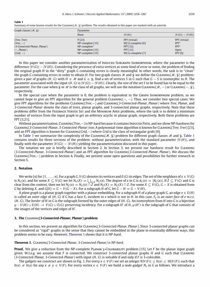
Fig. 1. A node-gadget and a connection in G, and the corresponding subgraphs of H used in the proof of Theorem 1.

central vertex ax, together with a cycle consisting of the vertices bx0, bx1, . . . , b

x6b(x)−1 with each b

xi being connected to a

x, andfinally the vertices cx0, . . . , c

x3b(x)−1with each c

xi being connected to three consecutive vertices from the cycle b

x0bx1 . . . b

x6b(x)−1,

as illustrated in Fig. 1. Formally, the edge set of the node-gadgetNx is {axbxj , bxj−1b

xj | j ∈ [6b(x)]}∪{c

xj bx2j, c

xj bx2j+1, c

xj bx2j+2|0 ≤

j < 3b(x)} where bx6b(x) = bx0. The node-gadget Nx can be considered as a plane graph, supposing that the verticesbx0, b

x1, . . . , b

x6b(x)−1 (and thus c

x0, c

x1, . . . , c

x3b(x)−1) are embedded in a clockwise order around a

x. We define the j-th blockBxj of Nx to be (c

x3j, c

x3j+1, c

x3j+2), for every 0 ≤ j < b(x). The type of c

xj can be 0, 1, or 2, according to the value of jmodulo 3.

We set Cx = {cxj |0 ≤ j < 3b(x)}.Let us fix an arbitrary ordering of the vertices of F . For each x < y with xy ∈ E(F) we build a connection Exy in G that

uses 9 consecutive blocks from each of Nx and Ny, say Bxi , . . . , Bxi+8 and B

yj , . . . , B

yj+8. These blocks are the base blocks for

Exy, and we also define b(x, y) = (i, j). Note that since b(x) ≥ 9|V (F)| > 9dF (x), we can define connections such thatno two connections share a common base block. To build Exy with b(x, y) = (i, j), we introduce new vertices dxy1 , d

xy2 , d

xy3

and edges {cx3i+26−6m+`dxym , c

y3j+6m−`d

xym |m ∈ [3], ` ∈ [6]} ∪ {cx3ic

y3j+24, c

x3i+4c

y3j+22, c

x3i+8c

y3j+20} (see Fig. 1). By choosing the

base blocks for each connection in a way that the order of the connections around a node-gadget is the same as the orderof the corresponding edges around the corresponding vertex for some fixed planar embedding of F , we can give a planarembedding of G. Moreover, it is easy to see that G is also 3-connected.To construct H , we make a disjoint copy G of G, and delete some edges and vertices from it as follows. For the copy of cxj

(ax, Cx, etc.) we write cxj (ax, Cx, etc. respectively). To get H , we delete from G the three edges connecting vertices of Cx and

Cy for every x < y and xy ∈ E(F), and also the vertices cx3j+1 and cx3j+2 for every x ∈ V (F), 0 ≤ j < b(x). Clearly, H is planar,

and observe that it remains 3-connected.Now, we prove that if Cleaning(3-Connected-Planar, 3-Connected-Planar) has a solution S for the input (H,G), then F

is 3-colorable. Let ϕ be an isomorphism from H to G − S. First, observe that since b(x) 6= b(y) if x 6= y, and the integers{b(x)|x ∈ V (F)} are large enough, ϕ must map ax to ax because of its degree. For each x ∈ V (F), the vertices in Cx \ S musthave the same type, so let the color of x be this type. If xy ∈ E(F), then the color of x and y must differ, otherwise one ofthe edges cx3ic

y3j+24, c

x3i+4c

y3j+22, c

x3i+8c

y3j+20 would be in G − S where b(x, y) = (i, j), as for every type t , one of these edges

connects two vertices of type t . Thus the coloring is proper.For the other direction, let t : V (F) → {0, 1, 2} be a coloring of F . For each x ∈ V (F), let S contain those vertices in

Cx whose type is not t(x). Let ϕ map ax and dxym (for every meaningful x, y,m) to ax and d

xym , respectively, and let ϕ map cxj

to cxj+t(x). By adjusting ϕ on the vertices bxi in the natural way, we can prove that ϕ is an isomorphism. It is clear that the

restriction of ϕ on Nx is an isomorphism. Note that the only vertex of Bxj present in G−S is cx3j+t(x) = ϕ(c

x3j), so independently

from t(x) and t(y), the neighborhood of dxym is also preserved. We only have to check that the edges connecting Cx and Cy arenot present in G − S. This is implied by the properness of the coloring, as all such edges connect vertices of the same type,but for xy ∈ E(F) the types of the vertices in Cx \ S and Cy \ S differ. �

We present an FPT algorithm for Cleaning(3-Connected-Planar, Planar) where the parameter is k = |V (G)| − |V (H)| forinput (H,G). We assume n = |V (H)| > k + 2 and n ≥ 4 as otherwise we can solve the problem by brute force. We alsoassume that H and G are simple graphs.Let S be a solution. First observe that if C is a set of at most 2 vertices such that G − C is not connected, then there is a

component K of G− C such that the 3-connected graph G− S is contained in G[V (K) ∪ C]. Clearly, |V (K)| ≥ n− 2, so K isunique by n > k+ 2. Since such a separating set C can be found in linear time [17], K can also be found in linear time. If nocomponent of G− C has size at least n− 2, the algorithm outputs ‘No’, otherwise it proceeds with G[V (K) ∪ C] as input.


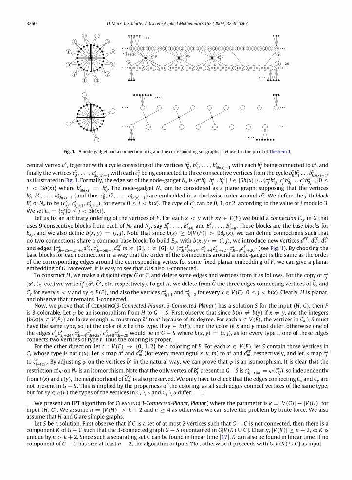
Fig. 2. Common neighbors test. Vertices ofM are indicated by double circles, and vertices of S by squares. By Lemma 2, we obtain that b ∈ S but a 6∈ S.

So we can assume that G is 3-connected. First the algorithm determines a planar embedding of H and G. Every planarembedding determines a circular order of the edges incident to a given vertex. Two embeddings are equivalent, if theseorderings are the same for each vertex in both of the embeddings. It is well known that a 3-connected planar graph hasexactly two planar embeddings, and these are reflections of each other (see e.g. [10]). Let us fix an arbitrary embedding θof H . By the 3-connectivity of G, one of the two possible embeddings of G yields an embedding of G − S that is equivalentto θ . The algorithm checks both possibilities. From now on, we regard H and G as plane graphs, and we are looking for anisomorphism ϕ from H into G− S which preserves the embedding.In a general step of the algorithm, we grow a partial mapping, which is a restriction of ϕ. We assume that ϕ is already

determined on a connected subgraph D of H having at least one edge. The definition of D implies ϕ(V (D)) ∩ S = ∅, so if atsome point the algorithm would have to delete vertices from ϕ(D), it outputs ‘No’.The algorithm grows the subgraph D on which ϕ is determined step by step. At each step, it chooses an outer edge e of

(D,H), and either deletes some vertices of G − ϕ(D) that must be in S, or adds to D an outer face F of e w.r.t. (D,H). Thealgorithm chooses e and F in a way such that after the first step the following property will always hold:

Invariant 1: the outer edges of (D,H) form a cycle.

We refer to this as choosing a suitable face. Formally, a face F is suitable for (D,H) if it is an outer face w.r.t. (D,H) andInvariant 1 holds after adding F toD. Lemma 1 argues that a suitable face can always be found.Wewill see that the algorithmcan only add a face F to D if ϕ(F) is a face of G as well (that is, the interior of ϕ(F) does not contain vertices from S). Hence,this method ensures that all vertices of ϕ(V (H − D)) and S are embedded on the same side of the border of ϕ(D), allowingus to assume the following:

Invariant 2: the vertices of V (G) \ ϕ(V (D)) are embedded in the unique unbounded region determined by the borderof ϕ(D) in G.

The most important consequence of Invariant 2 is that ϕ yields a bijection between the outer edges of (D,H) and the outeredges of (ϕ(D),G).

Lemma 1. If D is a subgraph of a 3-connected graph H such that |V (D)| < |V (H)| and the border of D in H is a cycle C, thenthere exists a suitable face for (D,H).

Proof. By |V (D)| < |V (H)|, each edge of C has an outer face w.r.t. (D,H). The planarity of H implies that if a, b, c, d are fourvertices appearing in this order on C , then there cannot exist two outer faces F1, F2 of (D,H) such that F1 contains a and c ,and F2 contains b and d. Given an outer face F of (D,H), let the gap of F be the maximum length of a subpath of C whoseendpoints are in V (F) but has no internal vertices in V (F).Now, consider an outer face F∗ of (D,H) that has minimum gap. If the gap of F∗ is at least 2, then there is a subpath Q of

C having at least two edges such that V (F∗)∩V (C) contains exactly the endpoints of Q . Consider any outer face FQ of (D,H)that is incident to an edge of Q . By the observation of the previous paragraph, such a face cannot be incident to a vertex of Cthat is not in Q . Thus, FQ must have smaller gap than F∗, which contradicts to the minimality of F∗. Therefore, F∗ must havegap 1. Hence, the vertices of V (F∗) ∩ V (C) are consecutive vertices of C , implying that F∗ is suitable. �

To find an initial partial mapping, we try to find a pair of edges ab and a′b′ in H and G, respectively, such that ϕ(a) = a′and ϕ(b) = b′. To do that, the algorithm fixes an arbitrary edge ab in H and guesses ϕ(a) and ϕ(b). This yields 2|E(G)|possibilities. After this, the algorithm applies one of the following steps.3-connectivity test. Although in the beginning G is assumed to be 3-connected, the algorithm may delete vertices from Gthroughout its running, and thus it can happen that G ceases to be 3-connected. This can be handled as described above, byfinding a separating set C of size at most 2, and determining the component K of G− C with at least |V (H)| − 2 vertices. Ifno such component exists, or if it does not include ϕ(D), then the algorithm outputs ‘No’, otherwise it deletes V (G−C −K).Common neighbors test. Let M = {ϕ(v)|v ∈ V (D), dH(v) < dG(ϕ(v))}. First, note that every vertex in M must have aneighbor in S, thus if |M| > 2k, then some vertex in S is adjacent to at least three vertices inM . By Invariant 2, the verticesof S ⊆ V (G) \ ϕ(V (D)) are embedded in the unbounded region determined by the border of ϕ(D) in G, the vertices of Mlie on this border. The algorithm checks every vertex q ∈ V (G) \ ϕ(V (D)) having at least three neighbors on the border ofϕ(D), and determines whether q ∈ S, using Lemma 2 below. If no such vertex of S can be found in spite of |M| > 2k, thenthe algorithm outputs ‘No’. Fig. 2 shows an example.


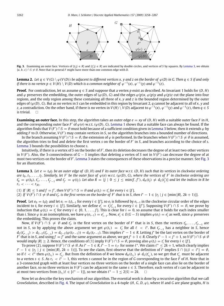
Fig. 3. Examining an outer face. Vertices of {tj|j ∈ R} and {t ′j |j ∈ R} are indicated by double circles, and vertices of S by squares. By Lemma 3, we obtain{a, b, c} ∩ S 6= ∅. Note that in general F might have more than one common edge with D.

Lemma 2. Let q ∈ V (G) \ ϕ(V (D)) be adjacent to different vertices x, y and z on the border of ϕ(D) in G. Then q ∈ S if and onlyif there is no vertex p ∈ V (H) \ V (D) which is a common neighbor of ϕ−1(x), ϕ−1(y) and ϕ−1(z).

Proof. For contradiction, let us assume q ∈ S and suppose that a vertex p exist as described. As Invariant 1 holds for (D,H)and ϕ preserves the embedding, the outer edges of (ϕ(D),G) and the edges ϕ(p)x, ϕ(p)y and ϕ(p)z cut the plane into fourregions, and the only region among these containing all three of x, y and z is the bounded region determined by the outeredges of (ϕ(D),G). But as no vertex in S can be embedded in this region by Invariant 2, q cannot be adjacent to all of x, y andz, a contradiction. On the other hand, if there is no vertex in V (H) \ V (D) adjacent to ϕ−1(x), ϕ−1(y) and ϕ−1(z), then q ∈ Sis trivial. �

Examining an outer face. In this step, the algorithm takes an outer edge e = xy of (D,H)with a suitable outer face F in H ,and the corresponding outer face F ′ of ϕ(e)w.r.t. (ϕ(D),G). Lemma 1 shows that a suitable face can always be found. If thealgorithm finds that V (F ′)∩ S = ∅must hold because of a sufficient condition given in Lemma 3 below, then it extends ϕ byadding F to D. Otherwise, V (F ′)may contain vertices in S, so the algorithm branches into a bounded number of directions.In the branch assuming V (F ′)∩ S = ∅, the extension of ϕ is performed. In the branches when V (F ′)∩ S 6= ∅ is assumed,

the algorithm tries to find and delete the first vertex s on the border of F ′ in S, and branches according to the choice of s.Lemma 3 bounds the possibilities to choose s.Intuitively, if there is a vertex of S on the border of F ′, then its deletion decreases the degree of at least two other vertices

in V (F ′). Also, the 3-connectedness of G − S implies that deleting a vertex of S not in V (F ′) can decrease the degree of atmost two vertices on the border of F ′. Lemma 3 states the consequences of these observations in a precise manner. See Fig. 3for an illustration.

Lemma 3. Let e = t0tf be an outer edge of (D,H) and F its outer face w.r.t. (D,H) such that its vertices in clockwise orderingare t0, t1, . . . , tf . Similarly, let F ′ be the outer face of ϕ(e) w.r.t. (ϕ(D),G), where the vertices of F ′ in clockwise ordering aret ′0 = ϕ(t0), t ′1, . . . , t

′

f ′−1 and t′

f ′ = ϕ(tf ). Let also R = {j | 0 ≤ j ≤ min(f , f ′), dH(tj) 6= dG(t ′j )} and let the indices in R ber1 < · · · < r|R|.

(1) If |R| ≤ 1 and f = f ′, then V (F ′) ∩ S = ∅ and ϕ(ti) = t ′i for every i ∈ [f ].(2) If V (F ′) ∩ S 6= ∅ and t ′i∗ is the first vertex on the border of F

′ that is in S, then i∗ − 1 ∈ {rj | j ∈ [min(|R|, 2k+ 1)]}.

Proof. Let e0 = t0tf and let ei = titi−1 for every i ∈ [f ], so ei is followed by ei−1 in the clockwise circular order of the edgesincident to ti for every i ∈ [f ]. Similarly, we define e′i = t

′

i t′

i−1 for every i ∈ [f′]. Supposing V (F ′) ∩ S = ∅, we prove by

induction that ϕ(ti) = t ′i for every i ∈ {0, 1, . . . , f }. This is clear for i = 0, so assume that it holds for each index smallerthan i. Since ϕ is an isomorphism, we have ϕ(ei−1) = e′i−1. Now, e

′

i ∈ E(G− S) implies ϕ(ei) = e′

i as well, since ϕ preservesthe embedding. This proves the claim.Now, if V (F ′) ∩ S 6= ∅ and t ′i∗ is the first vertex on the border of F

′ that is in S, then the vertices t ′0, . . . , t′

i∗−1 arenot in S, so by applying the above argument we get ϕ(t`) = t ′` for all ` < i∗. But t ′i∗−1 has a neighbor in S, hencedG(t ′i∗−1) > dG−S(t

′

i∗−1) = dG−S(ϕ(ti∗−1)) = dH(ti∗−1). This implies i∗− 1 ∈ R. Letting j∗ be the last vertex on the border of

F ′ that is in S, and using f = f ′ and the same argument as above, we get j∗+ 1 ∈ R. Clearly i∗− 1 < j∗+ 1, so V (F ′)∩ S 6= ∅would imply |R| ≥ 2. Hence, the conditions of (1) imply V (F ′) ∩ S = ∅, proving also ϕ(ti) = t ′i for every i ∈ [f ].To prove (2), suppose V (F ′)∩ S 6= ∅. As i∗− 1 ∈ R, i∗− 1 = r`∗ for some `∗. We claim `∗ ≤ 2k+ 1, which clearly implies

i∗ − 1 ∈ {rj | j ∈ [min(|R|, 2k + 1)]}. To see the claim, first observe that the definition of i∗ implies S ∩ {ti|i < i∗} = ∅,so if ` < `∗ then ϕ(tr`) = t

′r` . But from the definition of R we know dH(tr`) 6= dG(t

′r`), so we get that t

′r` must be adjacent

to a vertex s ∈ S. As r` < i∗ − 1, this vertex s cannot be in the region of G corresponding to the face F of H . Note that ina 3-connected graph with at least four vertices no three vertices on the border of a single face can also lie on the border ofanother face, so no three vertices in V (F ′) can be adjacent to the same s ∈ S. Therefore, each vertex of s can be adjacent toat most two vertices from {tr` |` ∈ [`

∗− 1]}, so we obtain `∗ − 1 ≤ 2|S| = 2k. �

Now let us describe the keymechanism of our algorithm. The essential work is done by a recursive algorithm that we callGrowSolution, described in Fig. 4. The input of GrowSolution is a 4-tuple (H,G,D, ϕ), where H and G are plane graphs, H is


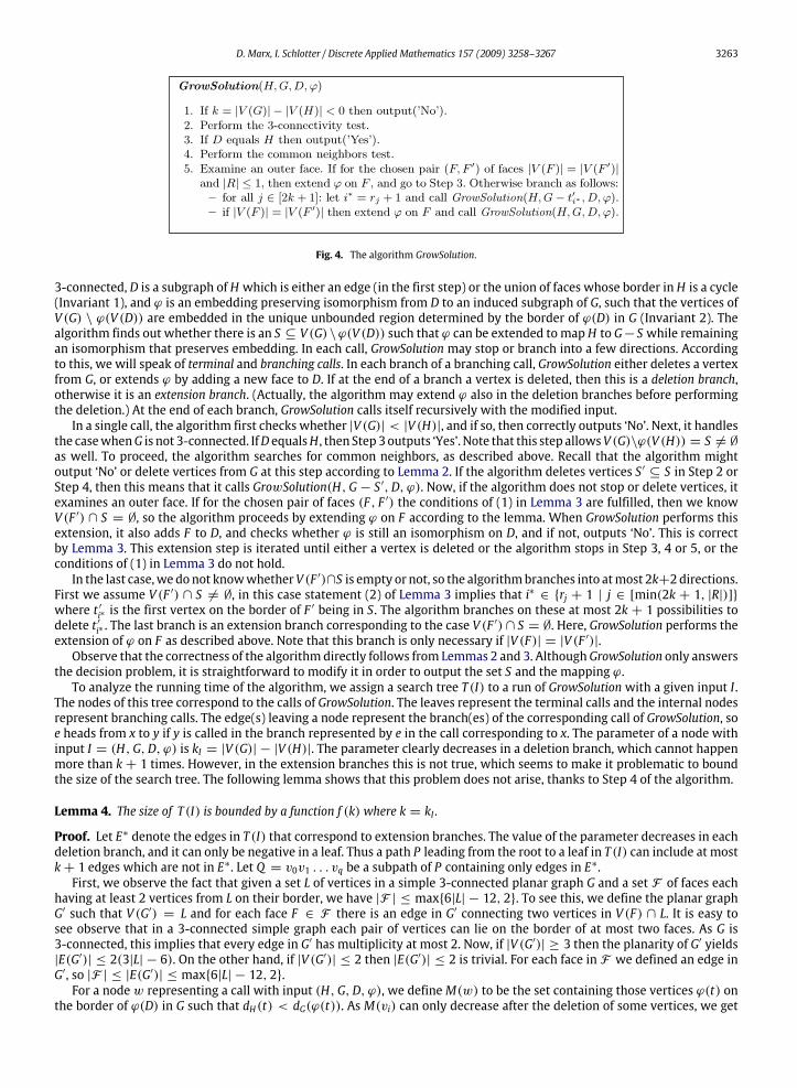
Fig. 4. The algorithm GrowSolution.

3-connected, D is a subgraph of H which is either an edge (in the first step) or the union of faces whose border in H is a cycle(Invariant 1), and ϕ is an embedding preserving isomorphism from D to an induced subgraph of G, such that the vertices ofV (G) \ ϕ(V (D)) are embedded in the unique unbounded region determined by the border of ϕ(D) in G (Invariant 2). Thealgorithm finds out whether there is an S ⊆ V (G)\ϕ(V (D)) such that ϕ can be extended to map H to G− S while remainingan isomorphism that preserves embedding. In each call, GrowSolutionmay stop or branch into a few directions. Accordingto this, we will speak of terminal and branching calls. In each branch of a branching call, GrowSolution either deletes a vertexfrom G, or extends ϕ by adding a new face to D. If at the end of a branch a vertex is deleted, then this is a deletion branch,otherwise it is an extension branch. (Actually, the algorithm may extend ϕ also in the deletion branches before performingthe deletion.) At the end of each branch, GrowSolution calls itself recursively with the modified input.In a single call, the algorithm first checks whether |V (G)| < |V (H)|, and if so, then correctly outputs ‘No’. Next, it handles

the casewhenG is not 3-connected. IfD equalsH , then Step3outputs ‘Yes’. Note that this step allowsV (G)\ϕ(V (H)) = S 6= ∅as well. To proceed, the algorithm searches for common neighbors, as described above. Recall that the algorithm mightoutput ‘No’ or delete vertices from G at this step according to Lemma 2. If the algorithm deletes vertices S ′ ⊆ S in Step 2 orStep 4, then this means that it calls GrowSolution(H,G− S ′,D, ϕ). Now, if the algorithm does not stop or delete vertices, itexamines an outer face. If for the chosen pair of faces (F , F ′) the conditions of (1) in Lemma 3 are fulfilled, then we knowV (F ′) ∩ S = ∅, so the algorithm proceeds by extending ϕ on F according to the lemma. When GrowSolution performs thisextension, it also adds F to D, and checks whether ϕ is still an isomorphism on D, and if not, outputs ‘No’. This is correctby Lemma 3. This extension step is iterated until either a vertex is deleted or the algorithm stops in Step 3, 4 or 5, or theconditions of (1) in Lemma 3 do not hold.In the last case,we donot knowwhetherV (F ′)∩S is empty or not, so the algorithmbranches into atmost 2k+2directions.

First we assume V (F ′) ∩ S 6= ∅, in this case statement (2) of Lemma 3 implies that i∗ ∈ {rj + 1 | j ∈ [min(2k + 1, |R|)]}where t ′i∗ is the first vertex on the border of F

′ being in S. The algorithm branches on these at most 2k + 1 possibilities todelete t ′i∗ . The last branch is an extension branch corresponding to the case V (F

′)∩ S = ∅. Here, GrowSolution performs theextension of ϕ on F as described above. Note that this branch is only necessary if |V (F)| = |V (F ′)|.Observe that the correctness of the algorithmdirectly follows from Lemmas 2 and 3. AlthoughGrowSolution only answers

the decision problem, it is straightforward to modify it in order to output the set S and the mapping ϕ.To analyze the running time of the algorithm, we assign a search tree T (I) to a run of GrowSolution with a given input I .

The nodes of this tree correspond to the calls of GrowSolution. The leaves represent the terminal calls and the internal nodesrepresent branching calls. The edge(s) leaving a node represent the branch(es) of the corresponding call of GrowSolution, soe heads from x to y if y is called in the branch represented by e in the call corresponding to x. The parameter of a node withinput I = (H,G,D, ϕ) is kI = |V (G)| − |V (H)|. The parameter clearly decreases in a deletion branch, which cannot happenmore than k + 1 times. However, in the extension branches this is not true, which seems to make it problematic to boundthe size of the search tree. The following lemma shows that this problem does not arise, thanks to Step 4 of the algorithm.

Lemma 4. The size of T (I) is bounded by a function f (k) where k = kI .

Proof. Let E∗ denote the edges in T (I) that correspond to extension branches. The value of the parameter decreases in eachdeletion branch, and it can only be negative in a leaf. Thus a path P leading from the root to a leaf in T (I) can include at mostk+ 1 edges which are not in E∗. Let Q = v0v1 . . . vq be a subpath of P containing only edges in E∗.First, we observe the fact that given a set L of vertices in a simple 3-connected planar graph G and a set F of faces each

having at least 2 vertices from L on their border, we have |F | ≤ max{6|L| − 12, 2}. To see this, we define the planar graphG′ such that V (G′) = L and for each face F ∈ F there is an edge in G′ connecting two vertices in V (F) ∩ L. It is easy tosee observe that in a 3-connected simple graph each pair of vertices can lie on the border of at most two faces. As G is3-connected, this implies that every edge in G′ has multiplicity at most 2. Now, if |V (G′)| ≥ 3 then the planarity of G′ yields|E(G′)| ≤ 2(3|L| − 6). On the other hand, if |V (G′)| ≤ 2 then |E(G′)| ≤ 2 is trivial. For each face in F we defined an edge inG′, so |F | ≤ |E(G′)| ≤ max{6|L| − 12, 2}.For a nodew representing a call with input (H,G,D, ϕ), we defineM(w) to be the set containing those vertices ϕ(t) on

the border of ϕ(D) in G such that dH(t) < dG(ϕ(t)). As M(vi) can only decrease after the deletion of some vertices, we get


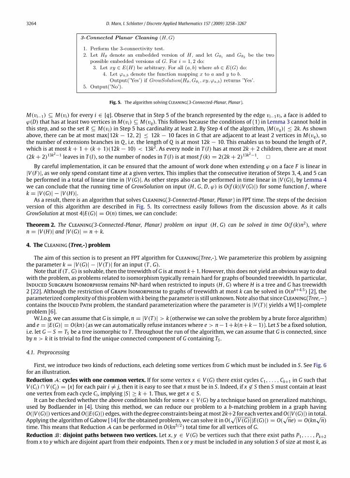
Fig. 5. The algorithm solving Cleaning(3-Connected-Planar, Planar).

M(vi−1) ⊆ M(vi) for every i ∈ [q]. Observe that in Step 5 of the branch represented by the edge vi−1vi, a face is added toϕ(D) that has at least two vertices inM(vi) ⊆ M(vq). This follows because the conditions of (1) in Lemma 3 cannot hold inthis step, and so the set R ⊆ M(vi) in Step 5 has cardinality at least 2. By Step 4 of the algorithm, |M(vq)| ≤ 2k. As shownabove, there can be at most max{12k − 12, 2} ≤ 12k − 10 faces in G that are adjacent to at least 2 vertices in M(vq), sothe number of extensions branches in Q , i.e. the length of Q is at most 12k − 10. This enables us to bound the length of P ,which is at most k + 1 + (k + 1)(12k − 10) < 13k2. As every node in T (I) has at most 2k + 2 children, there are at most(2k+ 2)13k

2−1 leaves in T (I), so the number of nodes in T (I) is at most f (k) = 2(2k+ 2)13k

2−1. �

By careful implementation, it can be ensured that the amount of work done when extending ϕ on a face F is linear in|V (F)|, as we only spend constant time at a given vertex. This implies that the consecutive iteration of Steps 3, 4, and 5 canbe performed in a total of linear time in |V (G)|. As other steps also can be performed in time linear in |V (G)|, by Lemma 4we can conclude that the running time of GrowSolution on input (H,G,D, ϕ) is O(f (k)|V (G)|) for some function f , wherek = |V (G)| − |V (H)|.As a result, there is an algorithm that solves Cleaning(3-Connected-Planar, Planar) in FPT time. The steps of the decision

version of this algorithm are described in Fig. 5. Its correctness easily follows from the discussion above. As it callsGrowSolution at most 4|E(G)| = O(n) times, we can conclude:

Theorem 2. The Cleaning(3-Connected-Planar, Planar) problem on input (H,G) can be solved in time O(f (k)n2), wheren = |V (H)| and |V (G)| = n+ k.

4. The Cleaning (Tree,-) problem

The aim of this section is to present an FPT algorithm for Cleaning(Tree,-). We parameterize this problem by assigningthe parameter k = |V (G)| − |V (T )| for an input (T ,G).Note that if (T ,G) is solvable, then the treewidth of G is at most k+1. However, this does not yield an obviousway to deal

with the problem, as problems related to isomorphism typically remain hard for graphs of bounded treewidth. In particular,Induced Subgraph Isomorphism remains NP-hard when restricted to inputs (H,G) where H is a tree and G has treewidth2 [22]. Although the restriction of Graph Isomorphism to graphs of treewidth at most k can be solved in O(nk+4.5) [2], theparameterized complexity of this problemwith kbeing the parameter is still unknown.Note also that sinceCleaning(Tree,−)contains the Induced Path problem, the standard parameterization where the parameter is |V (T )| yields a W[1]-completeproblem [6].W.l.o.g. we can assume that G is simple, n = |V (T )| > k (otherwise we can solve the problem by a brute force algorithm)

and e = |E(G)| = O(kn) (as we can automatically refuse instances where e > n−1+ k(n+ k−1)). Let S be a fixed solution,i.e. let G− S = TS be a tree isomorphic to T . Throughout the run of the algorithm, we can assume that G is connected, sinceby n > k it is trivial to find the unique connected component of G containing TS .

4.1. Preprocessing

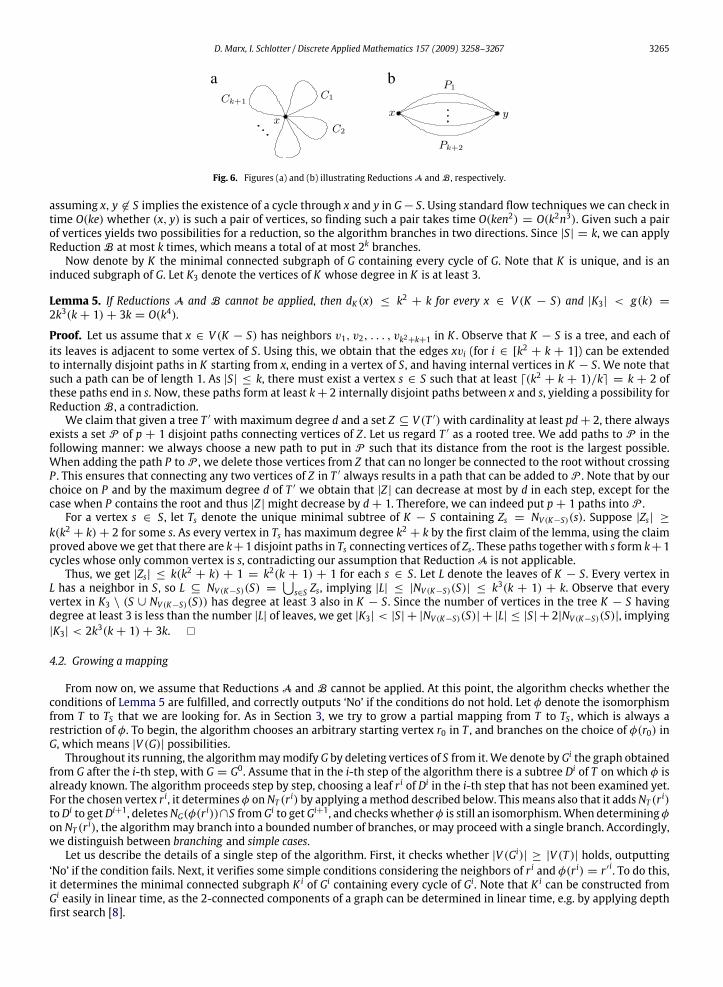
First, we introduce two kinds of reductions, each deleting some vertices from G which must be included in S. See Fig. 6for an illustration.Reduction A: cycles with one common vertex. If for some vertex x ∈ V (G) there exist cycles C1, . . . , Ck+1 in G such thatV (Ci) ∩ V (Cj) = {x} for each pair i 6= j, then it is easy to see that xmust be in S. Indeed, if x 6∈ S then S must contain at leastone vertex from each cycle Ci, implying |S| ≥ k+ 1. Thus, we get x ∈ S.It can be checked whether the above condition holds for some x ∈ V (G) by a technique based on generalized matchings,

used by Bodlaender in [4]. Using this method, we can reduce our problem to a b-matching problem in a graph havingO(|V (G)|) vertices andO(|E(G)|) edges,with the degree constraints being atmost 2k+2 for each vertex andO(|V (G)|) in total.Applying the algorithm of Gabow [14] for the obtained problem, we can solve it inO(

√|V (G)||E(G)|) = O(

√ne) = O(kn

√n)

time. This means that ReductionA can be performed in O(kn5/2) total time for all vertices of G.Reduction B: disjoint paths between two vertices. Let x, y ∈ V (G) be vertices such that there exist paths P1, . . . , Pk+2from x to ywhich are disjoint apart from their endpoints. Then x or ymust be included in any solution S of size at most k, as


a b

Fig. 6. Figures (a) and (b) illustrating ReductionsA andB, respectively.

assuming x, y 6∈ S implies the existence of a cycle through x and y in G− S. Using standard flow techniques we can check intime O(ke) whether (x, y) is such a pair of vertices, so finding such a pair takes time O(ken2) = O(k2n3). Given such a pairof vertices yields two possibilities for a reduction, so the algorithm branches in two directions. Since |S| = k, we can applyReductionB at most k times, which means a total of at most 2k branches.Now denote by K the minimal connected subgraph of G containing every cycle of G. Note that K is unique, and is an

induced subgraph of G. Let K3 denote the vertices of K whose degree in K is at least 3.

Lemma 5. If Reductions A and B cannot be applied, then dK (x) ≤ k2 + k for every x ∈ V (K − S) and |K3| < g(k) =2k3(k+ 1)+ 3k = O(k4).

Proof. Let us assume that x ∈ V (K − S) has neighbors v1, v2, . . . , vk2+k+1 in K . Observe that K − S is a tree, and each ofits leaves is adjacent to some vertex of S. Using this, we obtain that the edges xvi (for i ∈ [k2 + k + 1]) can be extendedto internally disjoint paths in K starting from x, ending in a vertex of S, and having internal vertices in K − S. We note thatsuch a path can be of length 1. As |S| ≤ k, there must exist a vertex s ∈ S such that at least d(k2 + k + 1)/ke = k + 2 ofthese paths end in s. Now, these paths form at least k+ 2 internally disjoint paths between x and s, yielding a possibility forReductionB, a contradiction.We claim that given a tree T ′ with maximum degree d and a set Z ⊆ V (T ′)with cardinality at least pd+ 2, there always

exists a set P of p + 1 disjoint paths connecting vertices of Z . Let us regard T ′ as a rooted tree. We add paths to P in thefollowing manner: we always choose a new path to put in P such that its distance from the root is the largest possible.When adding the path P toP , we delete those vertices from Z that can no longer be connected to the root without crossingP . This ensures that connecting any two vertices of Z in T ′ always results in a path that can be added to P . Note that by ourchoice on P and by the maximum degree d of T ′ we obtain that |Z | can decrease at most by d in each step, except for thecase when P contains the root and thus |Z |might decrease by d+ 1. Therefore, we can indeed put p+ 1 paths into P .For a vertex s ∈ S, let Ts denote the unique minimal subtree of K − S containing Zs = NV (K−S)(s). Suppose |Zs| ≥

k(k2 + k)+ 2 for some s. As every vertex in Ts has maximum degree k2 + k by the first claim of the lemma, using the claimproved above we get that there are k+1 disjoint paths in Ts connecting vertices of Zs. These paths together with s form k+1cycles whose only common vertex is s, contradicting our assumption that ReductionA is not applicable.Thus, we get |Zs| ≤ k(k2 + k) + 1 = k2(k + 1) + 1 for each s ∈ S. Let L denote the leaves of K − S. Every vertex in

L has a neighbor in S, so L ⊆ NV (K−S)(S) =⋃s∈S Zs, implying |L| ≤ |NV (K−S)(S)| ≤ k

3(k + 1) + k. Observe that everyvertex in K3 \ (S ∪ NV (K−S)(S)) has degree at least 3 also in K − S. Since the number of vertices in the tree K − S havingdegree at least 3 is less than the number |L| of leaves, we get |K3| < |S| + |NV (K−S)(S)| + |L| ≤ |S| + 2|NV (K−S)(S)|, implying|K3| < 2k3(k+ 1)+ 3k. �

4.2. Growing a mapping

From now on, we assume that Reductions A and B cannot be applied. At this point, the algorithm checks whether theconditions of Lemma 5 are fulfilled, and correctly outputs ‘No’ if the conditions do not hold. Let φ denote the isomorphismfrom T to TS that we are looking for. As in Section 3, we try to grow a partial mapping from T to TS , which is always arestriction of φ. To begin, the algorithm chooses an arbitrary starting vertex r0 in T , and branches on the choice of φ(r0) inG, which means |V (G)| possibilities.Throughout its running, the algorithmmaymodify G by deleting vertices of S from it.We denote by Gi the graph obtained

from G after the i-th step, with G = G0. Assume that in the i-th step of the algorithm there is a subtree Di of T on which φ isalready known. The algorithm proceeds step by step, choosing a leaf r i of Di in the i-th step that has not been examined yet.For the chosen vertex r i, it determines φ onNT (r i) by applying amethod described below. Thismeans also that it addsNT (r i)toDi to getDi+1, deletesNG(φ(r i))∩S fromGi to getGi+1, and checkswhetherφ is still an isomorphism.When determiningφon NT (r i), the algorithmmay branch into a bounded number of branches, or may proceed with a single branch. Accordingly,we distinguish between branching and simple cases.Let us describe the details of a single step of the algorithm. First, it checks whether |V (Gi)| ≥ |V (T )| holds, outputting

‘No’ if the condition fails. Next, it verifies some simple conditions considering the neighbors of r i and φ(r i) = r ′i. To do this,it determines the minimal connected subgraph K i of Gi containing every cycle of Gi. Note that K i can be constructed fromGi easily in linear time, as the 2-connected components of a graph can be determined in linear time, e.g. by applying depthfirst search [8].


To proceed, let us introduce some new notation. We divide the vertices of NT (r i) into two groups as follows:– those neighbors of r i that are in Di,– those neighbors of r i that are not in Di. Let t i1, . . . , t

iαidenote these vertices, and let T ij be the tree component of T − r

i

containing t ij .

Similarly, we classify the vertices of NG(r ′i) into three groups:

– those neighbors of r ′ i that are in φ(Di),– those neighbors of r ′ i outside φ(Di) that are connected to r ′ i by edges not in K i. Let t ′i1 , . . . , t

′iβ idenote these vertices, and

T ′ij denote the component of Gi− r ′ i that includes t ′ij . Observe that either T

′ij is a tree, or r

′ i6∈ V (K i) and T ′ij contains K

i.– those neighbors of r ′ i outside φ(Di) that are connected to r ′ i by edges in K i. Let γ i be the number of such vertices.

Clearly, αi ≤ β i+ γ i, and the equality holds if and only if NGi(r′i)∩ S = ∅. Thus, if the algorithm finds that αi > β i+ γ i,

then it outputs ‘No’.First, let us observe that if the tree T ih is isomorphic to T

′ij for some h and j, then w.l.o.g. we can assume that φ(T

ih) = T

′ij .

As the trees of a forest can be classified into equivalence classes with respect to isomorphism in time linear in the size of theforest [1,18], this case can be noticed easily. Given two isomorphic trees, an isomorphism between them can also be foundin linear time, so the algorithm can extend φ on T ih, adding also T

ih to the subgraph D

i. Hence, we only have to deal with thefollowing case: no tree T ih (h ∈ [α

i]) is isomorphic to one of the graphs T ′ij (j ∈ [β

i]). This argument makes our situation

significantly easier, since every graph T ′ij must contain some vertex from S. Therefore βi≤ |S| = k. Clearly, if r ′ i 6∈ V (K i)

then γ i = 0. On the other hand, if r ′ i ∈ V (K i) then r ′ i can have degree at most k2 + k in K 0, and thus in K i, by Lemma 5.Thus, we get γ i ≤ k2 + k, implying also αi ≤ β i + γ i ≤ k2 + 2k. The algorithm determines αi, β i and γ i in each step, andoutputs ‘No’ if these bounds do not hold for them.The algorithm faces one of the following two cases at each step.

Simple case: β i + γ i ≤ 1. In this case αi ≤ 1. If β i + γ i = 0 then αi = 0, hence the algorithm proceeds with the next stepby choosing another leaf of Di not yet visited. Otherwise, let v be the unique vertex in NGi(r

′i) \ V (φ(Di)). If αi = 0 then vmust be in S, otherwise φ(t i1) = v. According to this, the algorithm deletes v or extends φ on t

i1, adding also t

i1 to D

i.Branching case: β i + γ i ≥ 2. In this case, the algorithm branches on every possible choice of determining φ on NT (r i).Guessing φ(v) for a vertex v ∈ NV (T−Di)(r

i) can result in at most β i + γ i possibilities, so the number of possible branches ina branching step is at most (β i + γ i)α

i≤ (k2 + 2k)k

2+2k. After guessing φ(v) for each vertex v ∈ NV (T−Di)(r

i), the algorithmputs the remaining vertices NG(r ′

i) \ {φ(v)|v ∈ NT (r i)} into S, deleting them from Gi.

Lemma 6. In a single branch of a run of the algorithm described above on a solvable input for the Cleaning(Tree,-) problem withparameter k, there can be at most g(k)+ 2k− 2 branching steps.

Proof. We use the notation applied in the description of the algorithm. The i-th step can only be a branching case if eitherγ i ≥ 2, β i ≥ 2, or β i = γ i = 1 holds. For each of these cases, we give an upper bound on the number of steps in a singlebranch of a run of the algorithm where these cases can happen.To determine a bound for the case γ i ≥ 2, let r∗ be the first vertex in T examined in a step such that φ(r∗) is in K 0. Recall

that K 0 − S is a tree, so supposing φ(r i) ∈ V (K 0) we get that if r i 6= r∗ then for the edge e incident to r i in Di it must holdthat φ(e) is in K 0. Now, observe that if γ i ≥ 2 holds, then this implies that either r i = r∗ or φ(r i) has at least three edgesincident to it in K 0. The latter means that r i ∈ K3, where K3 denotes the vertices of K 0 having degree at least three in K 0.Thus, the condition γ i ≥ 2 can hold in at most |K3| + 1 ≤ g(k) steps, by Lemma 5.On the other hand, if the algorithm finds that β i ≥ 2, then recall that both T ′i1 and T

′i2 include at least one vertex from S,

and thus Gi − φ(Di) has more connected components containing vertices of S than Gi − φ(Di − r i) has. It is easy to see thatthis can be true for only at most |S| − 1 such vertices r i, so this case can happen at most k− 1 times in a single branch of arun of the algorithm.Finally, let S∗ denote those vertices of S that are not contained in K 0. Clearly, if s ∈ S∗, then s is not contained in any cycle

of G, so |NG(s) ∩ V (TS)| ≤ 1. Now, if β i = γ i = 1, then r ′i∈ V (K) and the edge r ′ it ′i1 must be one of the edges that connect

to K 0 a tree in G − K 0 containing a vertex in S∗. Observe that there can be at most |S∗| ≤ k − 1 such edges. Therefore, theclaim follows. �

As Lemma 6 only bounds the number of branching steps for solvable inputs, the algorithm ensures the same boundon every input by maintaining a counter for these steps. Thus, it outputs ‘No’ if it encounters a branching case for the(g(k)+ 2k− 1)-th time.At each vertex the algorithm uses time at most linear in |V (G)|. The number of steps performed is at most |V (T )|. As both

the number of branches in a branching case and the number of branching cases in a single branch of a run of the algorithmis bounded by a function of k, the algorithm needs quadratic time after choosing φ(r0) for the starting vertex r0. Trying allpossibilities on φ(r0) increases this to cubic time. ReductionsA andB can also be executed in cubic time, as argued before,so we can conclude:


Theorem 3. The Cleaning(Tree,-) problem on input (T ,G) can be solved in time O(f (k)n3), where n = |V (T )| and |V (G)| =n+ k.

5. Conclusions and open problems

We have investigated the complexity of the parameterized Cleaning (H,G) problem, where given two graphs H ∈ Hand G ∈ G with the parameter k = |V (G)| − |V (H)|, the task is to find k vertices in G whose deletion results in agraph isomorphic to H . We proved NP-completeness for the unparameterized version of the Cleaning problem in the casewhen both graphs are 3-connected planar graphs, and we presented FPT algorithms for the Cleaning(Tree,-) and Cleaning(3-Connected-Planar, Planar) problems.A natural question is whether the parameterized Cleaning(−, Planar) problem, or equivalently the Cleaning(Planar,

Planar) problem, is FPT with parameter |V (G)| − |V (H)|. It would be also interesting to determine the complexity of theCleaning problem for other graph classes for which the Graph Isomorphism problem can be solved in polynomial time,such as the class of interval graphs.Anotherway of generalization is to extend the set of allowed operationswhich can be used to clean the larger input graph

in order to obtain the smaller one. Such operations could involve the deletion of edges, or contraction of vertices or edges.By allowing the deletion of a certain number of vertices to be applied on the smaller graph also we obtain the MaximumCommon Induced Subgraph problem [19]. To our knowledge, none of these natural questions have been studied using thenon-standard parameterization examined in this paper.

Acknowledgment

We would like to thank an anonymous referee for pointing out an error in a previous version of the paper.

References

[1] A.V. Aho, J.E. Hopcroft, J.D. Ullman, The Design and Analysis of Computer Algorithms, Addison-Wesley, 1974.[2] H.L. Bodlaender, Polynomial algorithms for graph isomorphism and chromatic index on partial k-trees, J. Algorithms 11 (1990) 631–643.[3] H.L. Bodlaender, On disjoint cycles, Int. J. Found. Comput. Sci. 5 (1994) 59–68.[4] H.L. Bodlaender, A cubic kernel for feedback vertex set, in: STACS 2007, in: LNCS, vol. 4393, 2007, pp. 320–331.[5] L. Cai, S.M. Chan, S.O. Chan, Random separation: A new method for solving fixed-cardinality optimization problems, in: IWPEC 2006, in: LNCS,vol. 4169, 2006, pp. 239–250.

[6] Y. Chen, J. Flum, On parameterized path and chordless path problems, in: 22nd Annual IEEE Conference on Computational Complexity, 2007,pp. 250–263.

[7] Y. Chen, M. Thurley, W. Weyer, Understanding the complexity of induced subgraph isomorphisms, in: ICALP 2008, in: LNCS, vol. 5125, 2008,pp. 587–596.

[8] T.H. Cormen, C.E. Leiserson, R.L. Rivest, C. Stein, Introduction to Algorithms, second edition, MIT Press, 2001.[9] J. Díaz, D.M. Thilikos, Fast FPT-algorithms for cleaning grids, in: STACS 2006, in: LNCS, vol. 3884, 2006, pp. 361–371.[10] R. Diestel, Graph Theory, Springer, Berlin, 2000.[11] R.G. Downey, M.R. Fellows, Parameterized Complexity, Springer-Verlag, New York, 1999, Springer, 1999.[12] D. Eppstein, Subgraph isomorphism in planar graphs and related problems, J. Graph Algorithms Appl. 3 (3) (1999) 1–27.[13] J. Flum, M. Grohe, Parameterized Complexity Theory, Springer-Verlag, Berlin, 2006, Springer, 2006.[14] H.N. Gabow, An efficient reduction technique for degree-constrained subgraph and bidirected network flow problems, in: Proc. 15th Annual ACM

Symp. on Theory of Comp., 1983, pp. 448–456.[15] M.R. Garey, D.S. Johnson, Computers and Intractability. A Guide to the Theory of NP-Completeness, Freeman, San Francisco, 1979.[16] M.T. Hajiaghayi, N. Nishimura, Subgraph isomorphism, log-bounded fragmentation and graphs of (locally) bounded treewidth, J. Comput. Syst. Sci. 73

(5) (2007) 755–768.[17] J.E. Hopcroft, R.E. Tarjan, Dividing a graph into triconnected components, SIAM J. Comput. 2 (3) (1973) 135–158.[18] J.E. Hopcroft, R.E. Tarjan, Efficient planarity testing, J. Assoc. Comput. Mach. 21 (1974) 549–568.[19] X. Huang, J. Lai, Maximum common subgraph: Upper bound and lower bound results, in: IMSCCS 2006, vol. 1, pp. 40–47.[20] A. Lingas, Subgraph isomorphism for biconnected outerplanar graphs in cubic time, Theoret. Comput. Sci. 63 (3) (1989) 295–302.[21] D. Marx, I. Schlotter, Obtaining a planar graph by vertex deletion, in: WG 2007, in: LNCS, vol. 4769, 2007, pp. 292–303.[22] J. Matoušek, R. Thomas, On the complexity of finding iso- and other morphisms for partial k-trees, Discrete Math. 108 (1992) 343–364.[23] D. Matula, Subtree isomorphism in O(n5/2), Ann. Discrete Math. 2 (1978) 91–106.

Documents

Parameterized graph cleaning problems