Parameterized Model Order Reductionof Nonlinear Dynamical Systems

Brad BondResearch Laboratory in Electronics,

Massachusetts Institute of Technology,77 Massachusetts Ave, Cambridge, MA, 02139

Email: bnbond@mit.edu

Luca DanielResearch Laboratory in Electronics,

Massachusetts Institute of Technology,77 Massachusetts Ave, Cambridge, MA, 02139

Email: luca@mit.edu

Abstract— In this paper we present a parameterized reductiontechnique for non-linear systems. Our approach combines anexisting non-parameterized trajectory piecewise linear methodfor non-linear systems, with an existing moment matching param-eterized technique for linear systems. Results and comparisonsare presented for two examples: an analog non-linear circuit, anda MEM switch.

I. INTRODUCTION

The presence of several non-linear analog circuits andMicro-Electro-Mechanical (MEM) components in modernmixed signal System-on-Chips (SoC) makes the fully auto-matic synthesis and optimization of such systems an extremelychallenging task. The availability of techniques for generat-ing Parameterized Reduced Order Models (PROM) of non-linear dynamical systems could serve as a first step towardthe automatic and accurate characterization of geometricallycomplex components and subcircuits, eventually enabling theirsynthesis and optimization.

Several Parameterized Model Order Reduction techniqueshave been introduced in literature in the past few years. Someare based on statistical performance evaluation [1], [2], [3],[4], others are based on moment matching techniques [5],[6], [7], [8], [9], [10], or on Truncated Balance Realization(TBR) techniques [11], and on quasi-convex optimization tech-niques [12]. However, to our knowledge, almost all existingPMOR techniques apply only to linear systems. Very few, suchas [4], also apply to non-linear systems.

Several non-parameterized Model Order Reduction (MOR)approaches are available for non-linear systems. For instance,the reduction of weakly non-linear systems has been shownusing Volterra series and moment matching techniques [13],[14], [15], [16], [17], [18]. The reduction of strongly non-linear systems has been shown using Trajectory Piece-WiseLinear (TPWL) with moment matching techniques [19], [20],[21], [22], TPWL with TBR techniques [23], and trajectoryPieceWise Polynomial (PWP) with moment matching tech-niques [24], [25], [26]. However, to our knowledge, all existingmodel order reduction techniques for non-linear systems applyonly to non-parameterized systems.

The key contribution of this paper is the combination of anexisting non-parameterized trajectory piecewise linear methodfor non-linear systems, with an existing moment matching

parameterized technique for linear systems, hence introducinga parameterized reduction technique for non-linear systems.

The rest of the paper is organized as follows: In Sec-tion II we briefly review non-parameterized and parameter-ized reduction for linear systems using moment matching,and the trajectory piecewise linear reduction for non-linearnon-parameterized systems. In Section III we introduce ourmethod combining the two approaches. Three alternatives arepresented. In Section IV we demonstrate and compare ourtechniques modeling an analog circuit and a MEM switch.

II. BACKGROUND

A. Moment Matching MOR for Linear Systems

Consider a linear system

Edxdt

= Ax(t)+ bu(t), y(t) = cT x(t), (1)

where the state x has a very large order N. One approachto reduce the order of the system is to use an orthonormalprojection matrix V such that x≈Vx, where x is size q << N,obtaining

Edxdt

= Ax(t)+ bu(t), y(t) = cT x(t), (2)

where E = V T EV , A = V T AV , b = V T b, and cT = cTV [27].The projection matrix is carefully constructed to preserve theinput/output relationship (e.g. transfer function) of the system.For instance a projection matrix chosen such that

colspan(V )⊇ spanbM,MbM,M2bM, ...,Mq−1bM, (3)

would produce a reduced system matching the first q momentsof the Taylor Series expansion in the Laplace variable s of thelarge system transfer function [28],

x = [sI−M]−1bM u =∞

∑m=0

smMmbM u, (4)

where M = A−1E and bM =−A−1b.

B. Moment Matching PMOR for Linear Systems

Consider a linear system whose dynamical descriptor matri-ces in Laplace domain are functions of the Laplace frequencyvariable s, and of some other geometrical parameters, s1, ...,sµ,

E(s,s1, ...,sµ)x = bu, y = cT x. (5)

Using for instance a polynomial fitting technique,

E(s1, . . . ,sµ) = E0 +∑i

siEi +∑h,k

shskEh,k + . . .

and introducing additional parameters s as shown in [8], [9],

Ei =

Ei i = 0, . . . ,µEh,k h = 1, . . . ,µ; k = 1, . . . ,µ. . .

si =

si i = 1, . . . ,µshsk h = 1, . . . ,µ; k = 1, . . . ,µ. . .

one can approximate the parameterized system as

[E0 + s1E1 + ...+ spEp]x = bu (6)

Next, from the moments of the multivariable Taylor seriesexpansion

x =∞

∑m=0

(s1M1 + ...+ spMp)mbM u, (7)

a projection matrix, V , can be constructed such that

colspan(V )⊇ span

mq[m=0

m−(kp+···+k3)[k2=0

. . .m[

kp=0

Fmk2,...,kp

bM

(8)where bM = E−1

0 b, Mi =−E−10 Ei, and

Fmk2,...,kp

=

0 if ki ∈ 0,1, . . . ,m i = 2, . . . , p0 if k2 + · · ·+ kp ∈ 0,1, . . . ,mI if m = 0M1Fm−1

k2,...,kp+ · · ·+ MpFm−1

k2,...,kp−1 otherwise

In [8] it is shown that the reduced system

[V T E0V + s1V T E1V + · · ·+ spVT EpV ]x = V T bu (9)

y = cTV x,

assembled using such a projection matrix with q total columns,matches the first q moments (corresponding to the first mq

derivatives in each parameter) of the large system (6). Inthe same article it is also noted that, for a large number ofparameters p, and a modest number of derivatives mq matchedfor each parameter, this method generates systems of orderq = O(pmq).

C. TPWL for MOR of non-linear systems

Consider a non-linear system in the form

Edxdt

= A(x(t))+ bu(t), y = cT x(t). (10)

The Trajectory Piece-Wise Linear (TPWL) method [21] con-structs a collection of local linearizations, Ai x+Ki, of the non-linear function A(x(t)), around each of k linearization statesxi. The non-linear system is then approximated by weightedcombinations of the linear models,

Edxdt

=k

∑i=1

wi(x,X) [Aix + Ki]+ bu(t) (11)

where wi(x,X) are some weighting functions, which depend onthe state x, and on the k linearization points X = [x1,x2, ...,xk].Since covering the entire state space with linear approxima-tions would be extremely expensive, in the TPWL method thenon-linear system is simulated with some “typical” traininginputs, and only the trajectories of the state excited by thoseinputs are populated by linearized models (Ai,Ki). One majordrawback of this method is that the accuracy of the reducedmodel can be highly dependent on the “richness” of the inputschosen for training. Furthermore, exact training trajectories canbe in general expensive to generate since they involve simulat-ing the full non-linear system. In [20], [21] it was noted that analternative less expensive option for generating approximatetraining trajectories is to simulate only the partially createdreduced model, and to generate and add a new linearized andreduced model Ai whenever the reduced state x(t) strays morethan some distance δ from all the reduced centers xi of theprevious linearizations, i.e. when

mini||x(t)− xi||> δ. (12)

In all our experiments, so far, we have verified that approxi-mate training trajectory based approaches generate models asaccurate as exact training trajectory ones, hence we will adoptthis technique hereafter in this paper.

In the TPWL method, an orthonormal projection matrix Vis created by assembling all the column vectors produced byapplying (3) on each of the linearized models Ai. The finalreduced system is then

Edxdt

=k

∑i=1

wi(x, X)[Aix(t)+ Ki

]+ bu(t) (13)

where Ai =V T AiV , Ki =V T Ki, b =V T b, E =V T EV , x =V T x,X = [x1, ..., xk], and xi = V T xi. The relative weights, wi(x, X),of each linear model vary dynamically as the state evolves.One example of possible weighting functions is the one usedin [21],

wi(x, X) =exp

(−β ||x−xi||m

)

∑ki=1 exp

(−β ||x−xi||m

) , (14)

where β is some constant (typically we used 25), andm = mini ||x− xi||.

III. TPWL-PMOR

A system possessing a non-linear dependence on both thestate and some parameters may be of the form

Edxdt

= A(x(t),s1,s2, ...,sµ)+ bu(t) y(t) = cT x(t). (15)

Using a collection of local linearizations around different statesxi, as in II-C and [21], one obtains

Edxdt

=k

∑i=1

wi(x,X)[Ai(s1, ...,sµ)x(t)+ Ki(s1, ...,sµ)]+ bu(t).

(16)Using then, for instance, polynomial fitting, and introducingadditional parameters s j as in II-B and [8], [9] one obtains

Edxdt

=k

∑i=1

p

∑j=1

wi(x,X)s j[Ai jx(t)+ Ki j]+ bu(t) (17)

The resulting system is now described as a collection of klinear systems linearly dependent on p parameters. Henceone can use standard linear model order reduction techniques.For instance, using an orthonormal projection matrix V , thereduced system is

Edxdt

=k

∑i=1

p

∑j=1

wi(x, X)s j[Ai jx(t)+ Ki j]+ bu(t) (18)

y = cT x(t)

where E = V T EV , Ai j = V T Ai jV , Ki j = V T Ki j, b = V T b, cT =cTV , x(t) = V T x(t), X = [x1, ..., xk], and xi = V T xi.

In order to complete the procedure, two algorithms remainto be specified: how to choose the linearization points xi,and how to construct the projection matrix V . Alternativesfor each of such two tasks will now be discussed in detailsin Sections III-A and III-B. Combining different alternativeswill then produce in Section III-C our three proposed Non-Linear Parameterized Model Order Reduction (NLPMOR)algorithms.

A. Choosing Linearization Points

In the standard TPWL, the state linearization points arechosen along the state trajectories generated by applyingtypical training inputs. We can use here the same idea, and wewill refer to it as “training at a single point in the parameterspace”. However, one may notice that different trajectoriesmay be generated not only by varying the training inputs, butalso by training at different points in the parameter space. Wewill consider this option as well, and denote it as “training atmultiple points in the parameter space”.

The additional training trajectories introduced by training atmultiple points in the parameter space will increase the totalnumber k of linearized models, however it will not affect theorder q of the reduced system. Since the weighting functionsin equation (18) are typically non-zero for just a few modelsat any particular time, a larger set of linearized models is notexpected to significantly affect simulation time when using thereduced model.

B. Constructing Projection Matrix V

When constructing the orthonormal projection Matrix V ,one could simply ignore the dependency on geometrical pa-rameters, and assemble the columns of V as in the originalTPWL method, using the MOR vectors produced by apply-ing (3) on each of linearized models Ai. This procedure wouldproduced reduced models that match one single moment withrespect to each geometrical parameter. Hence we will denotethis procedure as a simple “MOR moment matching in V”.

However, as an alternative, one could also choose to usea multivariable Taylor series expansion about the Laplacevariable s and each of the geometrical parameters s j, andassemble the columns of V using the PMOR expression in (8).This procedure would produce reduced models that matchmore than one moment with respect to each set of geometricalparameter values. Hence we will denote this procedure as a“PMOR moment matching in V”.

Matching multiple moments about multiple expansionpoints in the parameter space, for every linearized modelmay quickly increase the number of columns q of the pro-jection matrix V , hence possibly affecting the reduced modelsimulation cost. In order to contain the final order q of thereduced model, one can use a Singular Value Decomposition(SVD) on V , and select its first q most relevant singularvectors, identified by its largest q singular values. Such SVDis relatively inexpensive since, although V can be very tall, itwill be in most cases not very wide.

C. Proposed TPWL-PMOR Algorithms

Combining the parameterization options in sections III-Aand III-B gives rise to four different algorithms, shown inTable I, for Trajectory PieceWise Linear Parameterized ModelOrder Reduction (TPWL-PMOR) of a non-linear system.

TABLE I

FOUR OPTIONS FOR PARAMETERIZED REDUCTION OF NON-LINEAR

SYSTEMS.

Training at Training atSingle Point in Multiple Points in

Parameter Space Parameter SpaceMOR

Moment Matching in V TPWL Algorithm 2PMOR

Moment Matching in V Algorithm 1 Algorithm 3

TPWL. One can note that using a simple non-parameterized“MOR moment matching in V”, while “training at a singlepoint in parameter space”, is equivalent to applying the alreadyavailable non-parameterized TPWL algorithm [21] on the pa-rameterized system (17). Hence we will denote this algorithmas “TPWL”, since it is just a very trivial extension of that wellknown algorithm.

Algorithm 1 Trained at Single Parameter Point with PMORMoment Matching Projection Matrix V

1: i← 12: for all training inputs do3: t← tinitial

4: while t < tfinal do5: if mini ‖ x(t)− xi ‖> δ then6: Linearize at current state xi← x(t)7: Generate PMOR vectors (8)8: Orthogonalize and add them to V9: Update reduced model using (18)

10: i← i+ 111: end if12: Simulate reduced model to next time step t13: end while14: end for15: Perform SVD on projection matrix V16: Update reduced model using (18)

Algorithm 2 Trained at Multiple Parameter Values with MORMoment Matching Projection Matrix V

1: i← 12: for all training points in the parameter space do3: for all training inputs do4: t← tinitial

5: while t < tfinal do6: if mini ‖ x(t)− xi ‖> δ then7: Linearize at current state xi← x(t)8: Generate MOR vectors (3)9: Orthogonalize and add them to V

10: Update reduced model using (18)11: i← i+ 112: end if13: Simulate reduced model to next time step t14: end while15: end for16: end for17: Perform SVD on projection matrix V18: Update reduced model using (18)

Algorithm 1. A more interesting case from Table I, isobtained by combining “PMOR moment matching in V”,while still “training at a single point in parameter space”.The resulting complete procedure is summarized in Algo-rithm 1. Compared to the previous TPWL case, Algorithm 1is potentially more expensive since many more vectors aregenerated (each requiring a system solve) in order to matchseveral moments with respect to each geometrical parameter.More precisely, O(kpmq) vectors need to be generated to matchmq moments with respect to each of the p parameters for klinearized models Ai. An SVD is then performed on V to keepthe final order q of the reduced system small.

Algorithm 3 Trained at Multiple Parameter Values withPMOR Moment Matching Projection Matrix V

1: i← 12: for all training points in the parameter space do3: for all training inputs do4: t← tinitial

5: while t < tfinal do6: if mini ‖ x(t)− xi ‖> δ then7: Linearize at current state xi← x(t)8: Generate PMOR vectors (8)9: Orthogonalize and add them to V

10: Update reduced model using (18)11: i← i+ 112: end if13: Simulate reduced model to next time step t14: end while15: end for16: end for17: Perform SVD on projection matrix V18: Update reduced model using (18)

Algorithm 2. Another case of interest in Table I, trains thesystem at multiple points in the parameter space. Reductionis then performed with a non-parameterized MOR momentmatching projection matrix V . The complete procedure isoutlined in Algorithm 2. The final system is now a collectionof linear models corresponding to different sets of parametervalues. Compared to TPWL, the additional cost in Algorithm 2lies in creating additional training trajectories. More specif-ically, training the system for p different parameters at rdifferent values requires generating rp additional trajectories.Constructing the projection matrix V now requires generatingO(kp) vectors (i.e. O(kp) system solves), although the numberk of linearized models Ai may be O(rp) times larger than inTPWL or in Algorithm 1.

Algorithm 3. In the forth and final case described in Table I,the system is trained at multiple points in the parameterspace, and the models are reduced with a PMOR momentmatching projection matrix V . The complete procedure issummarized in Algorithm 3. Compared to all the previousAlgorithms, a model created by Algorithm 3 can potentiallycover the largest region of the parameter space, however it isthe most expensive to build. Specifically, as in Algorithm 2,the number of additional training trajectories is O(rp). Theprojection matrix requires generating O(pmq rp) vectors (i.e.system solves), where pmq is the number of vectors created bymatching mq moments with respect to each parameter at eachof the rp sets of parameter values (i.e. training trajectories).

IV. EXAMPLES

Two examples were chosen to test the methods presented inSections III-C. Both examples are highly non-linear systemsand depend geometrically on several parameters.

A. Non-Linear Analog Circuit Example Description

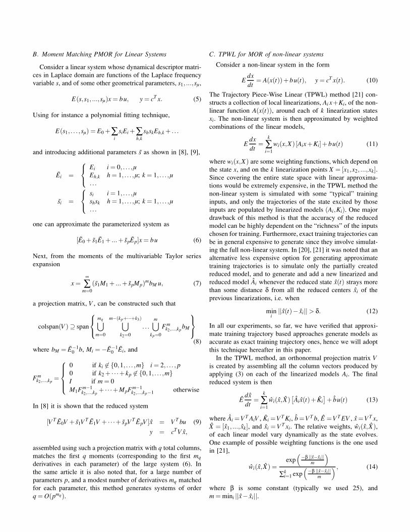
The first example considered is a non-linear analog circuitcontaining a chain of strongly non-linear diodes, together withresistors and capacitors as shown in Fig. 1 This examplewas first used by the authors in [21], [23] to illustrate thenon-parameterized TPWL-MOR method. By using the sameexample here we will try to compare the advantages of ourparameterized algorithms.

Fig. 1. A non-linear analog circuit example [21], [23]

The state of the system contains the nodal voltages,x(t) = [v1 v2 ... vN ]T , and the input is an ideal current sourceu(t) = i(t). The system equations are derived using Kirchoff’scurrent law and nodal analysis. An equation for interior nodej would be of the form,

Cdv j

dt=

1r

(v j−1−v j

)− 1r

(v j−v j+1

)+ Id

[eα(v j−1−v j)−eα(v j−v j+1)

]

leading to a state space system of the form

Edxdt

= Gx + D(x)+ bu(t). (19)

Here G is the conductance matrix, E is the capacitance matrix,D(x) is a vector valued non-linear function containing theconstitutive relations for the diodes, and b = [1 0 ...0]T is theinput vector. All resistors have value r = 1Ω, and all capacitorsare C = 10pF. The diodes have a constitutive relation

id(v) = Id(eαv−1), (20)

where α = 1/vt , and vT is the threshold voltage. Nominal val-ues for this device were Id = 0.1nA, and α = 40 (correspondingto vt = 25mV ).

The analog circuit was parameterized in both α and Id . Weapproximated the non-linear dependency on such parametersusing

Edxdt

= Gx + D(x,α0, Id0)+∂D(x,α0, Id0)

∂α(α−α0)+

+∂D(x,α0, Id0)

∂Id(Id− Id0)+ bu(t)

The model then produced at each linearization state xi, islinear both in the parameters and in the state, and has thesame frequency domain form as in (6):

sEx = Gx + Di + JDi · (x− xi)++Dαi · (α−α0)+ JDα · (α−α0) · (x− xi)++DId i · (Id− Id0)+ JDId · (Id− Id0) · (x− xi)+ bu(t),

where s is the Laplace variable, Di = D(xi,α0, Id0),JDi is the Jacobian of D(x,α0, Id0) with respect to x,Dαi = ∂D

∂α (xi,α0, Id0), JDα is the Jacobian of ∂D∂α with respect

to x, DId i = ∂D∂Id

(xi,α0, Id0), and JDId is the Jacobian of ∂D∂Id

withrespect to x.

Training trajectories were created with a sinusoidal input,u(t) = [cos(ωt)+ 1]/2, with ω = 2πGHz. When matching mo-ments with respect to frequency, both in MOR and in PMORwe used s0 = j2πGHz as a Taylor series expansion point.When matching moments with a simple non-parameterizedMOR projection matrix V , or when training at a single pointin parameter space, we evaluated the system at the nominalvalues α = 40, and Id = 0.1nA. When matching moments witha PMOR procedure, or when training at multiple moments inparameter space, we used α = 40, 50, and Id = 0.1nA, 0.3nA.

Results from this example are shown in Fig. 4, 5, 6, andwill be illustrated and discussed in details in the next Section.

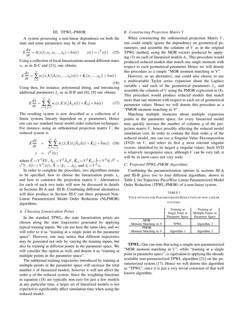
B. MEM Switch Example

The second example tested is a micromachined switch [21],[23]. The switch consists of a polysilicon fixed-fixed beamsuspended over a polysilicon pad on a silicon substrate asshown in Fig. 2. When a voltage is applied between the beamand the substrate, the electrostatic force generated pulls thebeam down toward the pad. If the force is great enough, thebeam will come into contact with the pad closing the circuit.The unknowns of interest in this system have been chosen tobe the deflection of the beam, z, and the air pressure betweenthe beam and substrate, p.

x

Si substrate

2 um of poly Si

0.5 um of poly Si deflection

2.3 um gap

filled with air0.5 um SiN

z

y

y(t) − center point

u=v(t)

Fig. 2. The MEMS switch is a polysilicon beam fixed at both ends andsuspended over a semiconducting pad and substrate [21], [23].

The system of equations was assembled by discretizing thecoupled 1D Euler’s Beam Equation (21), and the 2D Reynold’ssqueeze film damping equation (22), taken from [21]. A finitedifference scheme was used for the discretization, and sincethe length of the beam is much greater than the width, thevertical deflection was assumed to be uniform across the widthand only pressure was discretized in the width.

EI0h3w∂4z∂x4 −S0hw

∂2z∂x2 = Felec +

Z w

0(p− pa)dy−ρ0hw

∂2z∂t2 (21)

∇ · [(1+6K)z3 p ∇p]

= 12µ∂(pz)

∂t(22)

Here, Felec =−(ε0wv2)/(wz2) is the electrostatic force acrossthe plates resulting from the applied voltage v, while u = v2 isthe input to the system. The system output is the height of thebeam center point. The beam is 610µm in length, and has awidth of 40µm. The other constants are permittivity of freespace ε0 = 8.854 ∗ 10−6F/m, permeability µ = 4π ·10−7H/m,moment of inertia I0 = 1/12, Young’s modulus E = 149GPa,Knudsen number K = 0.064/z0, stress coefficient S0 =−3.7,and density ρ0 = 2300 kg /m3. By setting the state-space vari-ables to x1 = z, x2 = ∂z3

∂t , and x3 = p, the following dynamicalsystem results.

dx1

dt=

x2

3x21

dx2

dt=

2x22

3x31

+3x2

1

ρ0hw

[Z w

0(x3− pa)dy+S0hw

∂2x1

∂x2 −EIh3w∂4x1

∂x4

]− 3ε0

2ρ0hv2

dx3

dt= − x2x3

3x31

+1

12µx1∇

[(1+6

λx1

)x3

1x3∇x3

]

The beam is fixed at both ends and initially in equilibrium, sothe applied boundary conditions are

z(x,0) = z0, p(x,y,0) = pa, z(0,t) = z(l,t) = z0. (23)

Other constraints enforced are,

∂p(0,y, t)∂x

=∂p(l,y,t)

∂x= 0, p(x,0,t) = p(x,w,t) = pa (24)

The initial height and pressure used were z0 = 2.3µm, andpa = 1.103 ∗ 105Pa.

For this MEMS switch system, we are interested in produc-ing a model as a function of the width w. The dependency onthe parameter is easily made linear in this case by introducingvariable β = 1/w, and parameterizing the system with respectto β instead of w

dxdt

= A0(x)+ βA1(x)+ bu(t) (25)

Training trajectories were created using a step input,u(t) = v2 for t > 0, with v = 7. When matching momentswith a simple non-parameterized MOR projection matrix V ,or when training at a single point in parameter space, weevaluated the system at the nominal values β = 1/40. Whenmatching moments with a PMOR moment matching projectionmatrix V , or when training at multiple moments in parameterspace, we used β = 1/40,1/44.4.

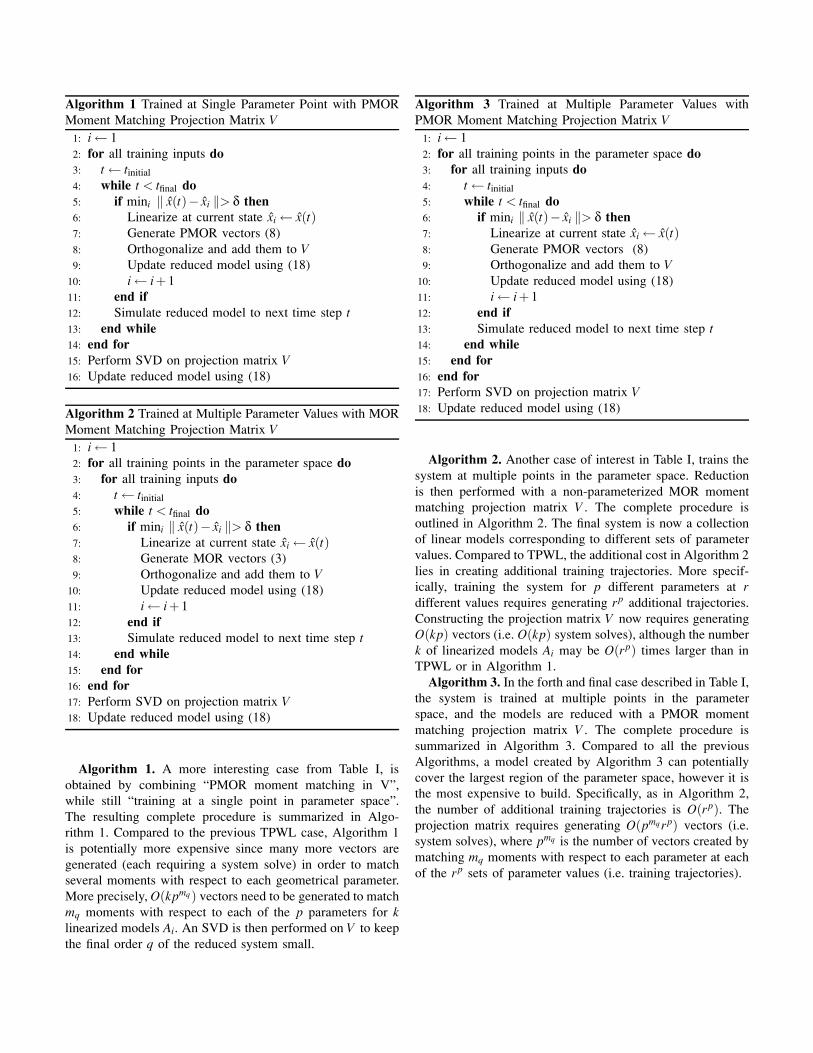
Results from this example are shown in Fig. 3 and will beillustrated and discussed in details in the next Section.

1 2 3 4 5 6

x 10−5

1.85

1.9

1.95

2

2.05

2.1

2.15

2.2

2.25

2.3

time

Pos

ition

MEM Switch Example −− Algorithm 1 vs Algorithm 3

Full Nonlinear Solutionat β = 1/43.24

Algorithm 3Algorithm 1

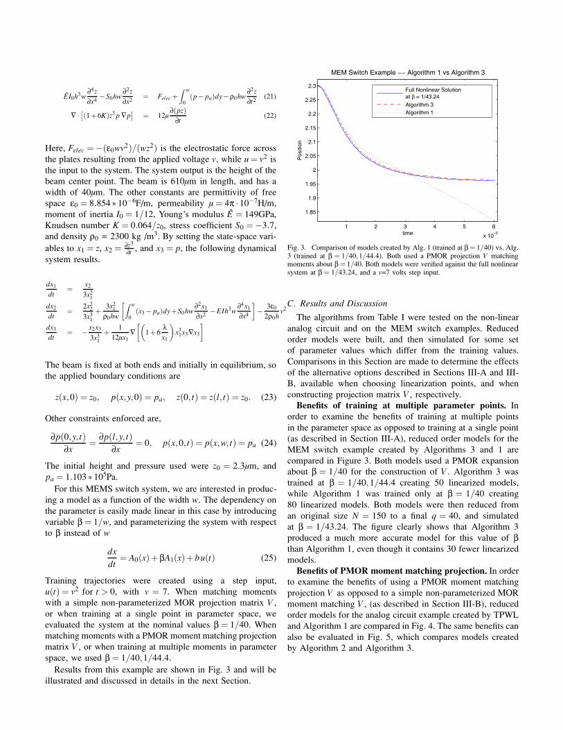
Fig. 3. Comparison of models created by Alg. 1 (trained at β = 1/40) vs. Alg.3 (trained at β = 1/40,1/44.4). Both used a PMOR projection V matchingmoments about β = 1/40. Both models were verified against the full nonlinearsystem at β = 1/43.24, and a v=7 volts step input.

C. Results and Discussion

The algorithms from Table I were tested on the non-linearanalog circuit and on the MEM switch examples. Reducedorder models were built, and then simulated for some setof parameter values which differ from the training values.Comparisons in this Section are made to determine the effectsof the alternative options described in Sections III-A and III-B, available when choosing linearization points, and whenconstructing projection matrix V , respectively.

Benefits of training at multiple parameter points. Inorder to examine the benefits of training at multiple pointsin the parameter space as opposed to training at a single point(as described in Section III-A), reduced order models for theMEM switch example created by Algorithms 3 and 1 arecompared in Figure 3. Both models used a PMOR expansionabout β = 1/40 for the construction of V . Algorithm 3 wastrained at β = 1/40,1/44.4 creating 50 linearized models,while Algorithm 1 was trained only at β = 1/40 creating80 linearized models. Both models were then reduced froman original size N = 150 to a final q = 40, and simulatedat β = 1/43.24. The figure clearly shows that Algorithm 3produced a much more accurate model for this value of βthan Algorithm 1, even though it contains 30 fewer linearizedmodels.

Benefits of PMOR moment matching projection. In orderto examine the benefits of using a PMOR moment matchingprojection V as opposed to a simple non-parameterized MORmoment matching V , (as described in Section III-B), reducedorder models for the analog circuit example created by TPWLand Algorithm 1 are compared in Fig. 4. The same benefits canalso be evaluated in Fig. 5, which compares models createdby Algorithm 2 and Algorithm 3.

12 14 16 18 20 22 24 26 28 30 320.5

1

1.5

2

2.5

3

3.5

4

Reduced Order

% E

rror

Circuit Example −− TPWL vs Algorithm 1

Algorithm 1TPWL

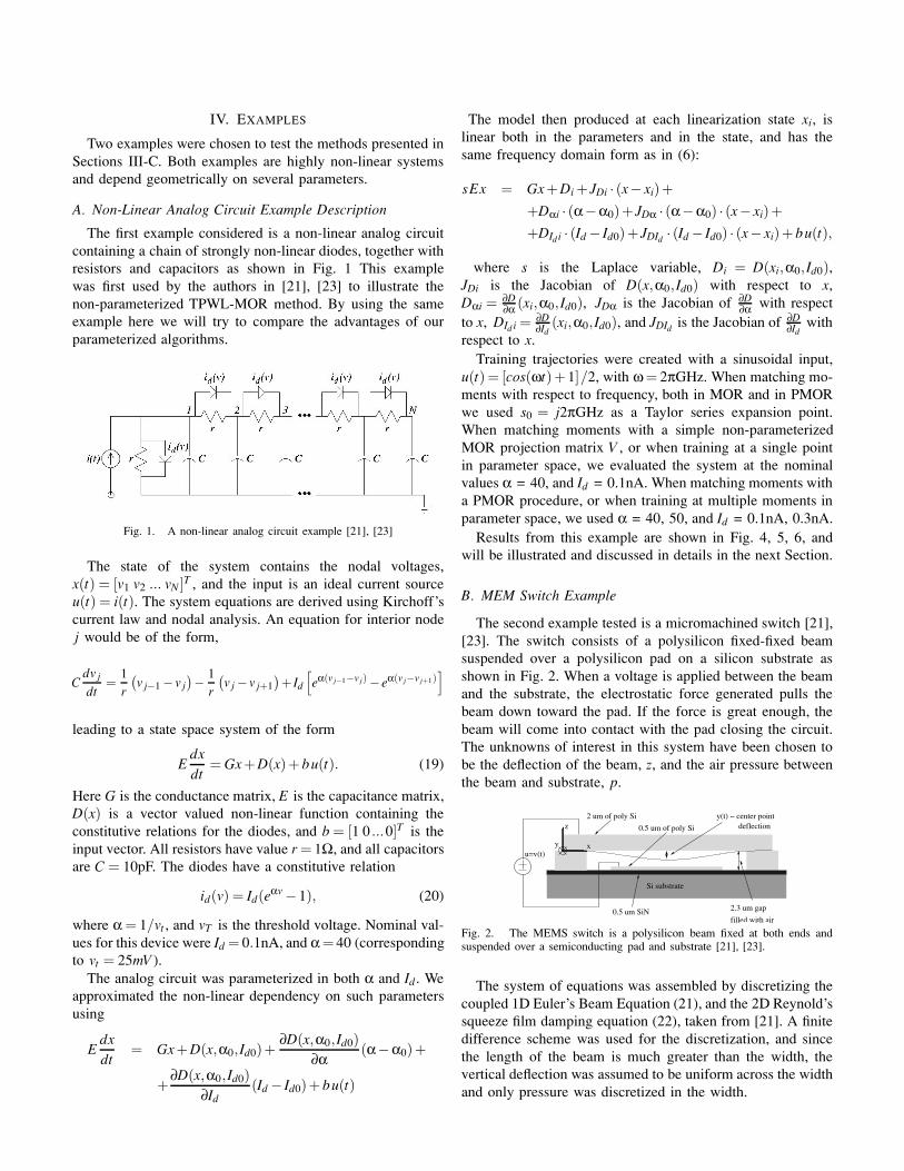
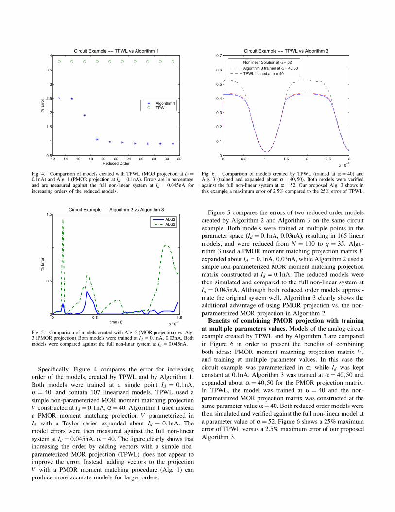
Fig. 4. Comparison of models created with TPWL (MOR projection at Id =0.1nA) and Alg. 1 (PMOR projection at Id = 0.1nA). Errors are in percentageand are measured against the full non-linear system at Id = 0.045nA forincreasing orders of the reduced models.

0 0.5 1 1.5

x 10−9

0

0.5

1

1.5

time (s)

% E

rror

Circuit Example −− Algorithm 2 vs Algorithm 3

ALG3ALG2

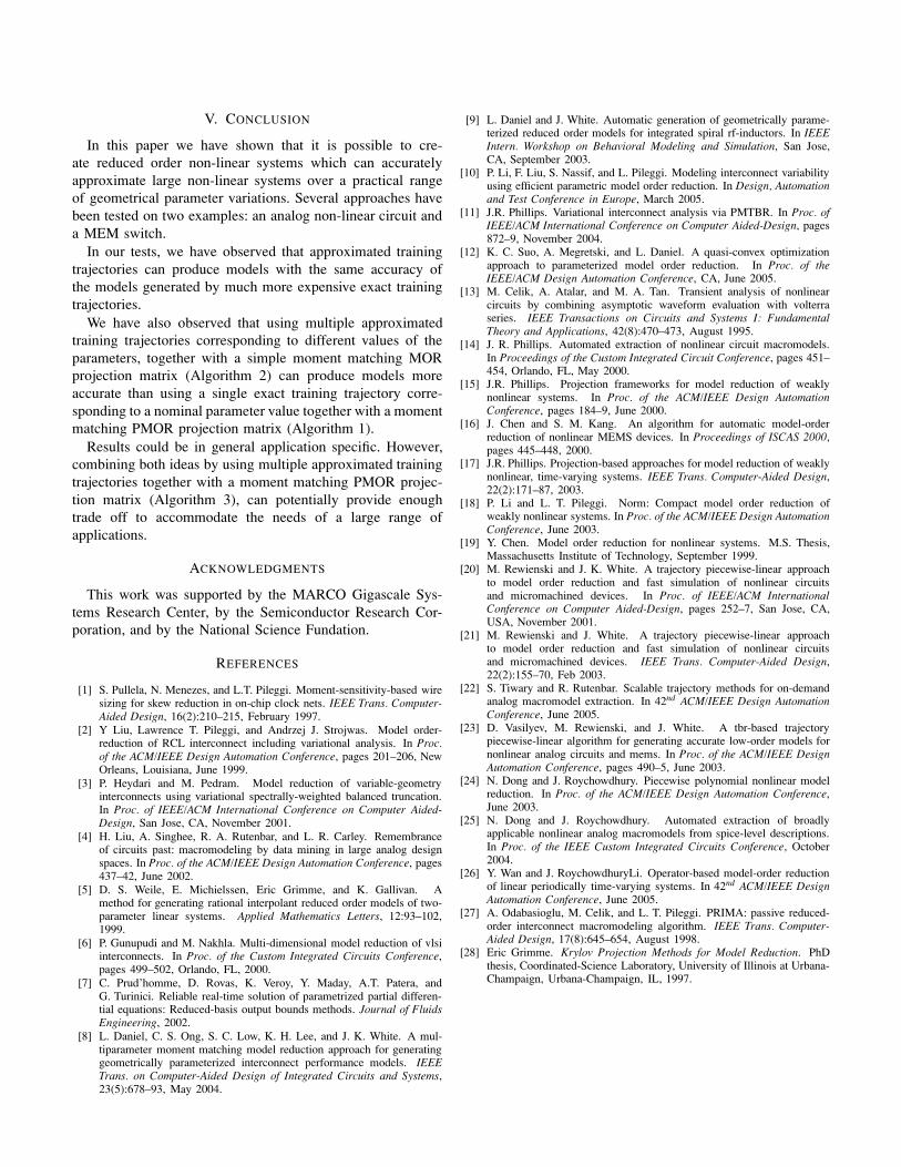
Fig. 5. Comparison of models created with Alg. 2 (MOR projection) vs. Alg.3 (PMOR projection) Both models were trained at Id = 0.1nA, 0.03nA. Bothmodels were compared against the full non-linar system at Id = 0.045nA.

Specifically, Figure 4 compares the error for increasingorder of the models, created by TPWL and by Algorithm 1.Both models were trained at a single point Id = 0.1nA,α = 40, and contain 107 linearized models. TPWL used asimple non-parameterized MOR moment matching projectionV constructed at Id = 0.1nA, α = 40. Algorithm 1 used insteada PMOR moment matching projection V parameterized inId with a Taylor series expanded about Id = 0.1nA. Themodel errors were then measured against the full non-linearsystem at Id = 0.045nA, α = 40. The figure clearly shows thatincreasing the order by adding vectors with a simple non-parameterized MOR projection (TPWL) does not appear toimprove the error. Instead, adding vectors to the projectionV with a PMOR moment matching procedure (Alg. 1) canproduce more accurate models for larger orders.

0 0.5 1 1.5 2 2.5 3

x 10−9

0

0.1

0.2

0.3

0.4

0.5

0.6

0.7Circuit Example −− TPWL vs Algorithm 3

Nonlinear Solution at α = 52

Algorithm 3 trained at α = 40,50

TPWL trained at α = 40

Fig. 6. Comparison of models created by TPWL (trained at α = 40) andAlg. 3 (trained and expanded about α = 40,50). Both models were verifiedagainst the full non-linear system at α = 52. Our proposed Alg. 3 shows inthis example a maximum error of 2.5% compared to the 25% error of TPWL.

Figure 5 compares the errors of two reduced order modelscreated by Algorithm 2 and Algorithm 3 on the same circuitexample. Both models were trained at multiple points in theparameter space (Id = 0.1nA, 0.03nA), resulting in 165 linearmodels, and were reduced from N = 100 to q = 35. Algo-rithm 3 used a PMOR moment matching projection matrix Vexpanded about Id = 0.1nA, 0.03nA, while Algorithm 2 used asimple non-parameterized MOR moment matching projectionmatrix constructed at Id = 0.1nA. The reduced models werethen simulated and compared to the full non-linear system atId = 0.045nA. Although both reduced order models approxi-mate the original system well, Algorithm 3 clearly shows theadditional advantage of using PMOR projection vs. the non-parameterized MOR projection in Algorithm 2.

Benefits of combining PMOR projection with trainingat multiple parameters values. Models of the analog circuitexample created by TPWL and by Algorithm 3 are comparedin Figure 6 in order to present the benefits of combiningboth ideas: PMOR moment matching projection matrix V ,and training at multiple parameter values. In this case thecircuit example was parameterized in α, while Id was keptconstant at 0.1nA. Algorithm 3 was trained at α = 40,50 andexpanded about α = 40,50 for the PMOR projection matrix.In TPWL, the model was trained at α = 40 and the non-parameterized MOR projection matrix was constructed at thesame parameter value α = 40. Both reduced order models werethen simulated and verified against the full non-linear model ata parameter value of α = 52. Figure 6 shows a 25% maximumerror of TPWL versus a 2.5% maximum error of our proposedAlgorithm 3.

V. CONCLUSION

In this paper we have shown that it is possible to cre-ate reduced order non-linear systems which can accuratelyapproximate large non-linear systems over a practical rangeof geometrical parameter variations. Several approaches havebeen tested on two examples: an analog non-linear circuit anda MEM switch.

In our tests, we have observed that approximated trainingtrajectories can produce models with the same accuracy ofthe models generated by much more expensive exact trainingtrajectories.

We have also observed that using multiple approximatedtraining trajectories corresponding to different values of theparameters, together with a simple moment matching MORprojection matrix (Algorithm 2) can produce models moreaccurate than using a single exact training trajectory corre-sponding to a nominal parameter value together with a momentmatching PMOR projection matrix (Algorithm 1).

Results could be in general application specific. However,combining both ideas by using multiple approximated trainingtrajectories together with a moment matching PMOR projec-tion matrix (Algorithm 3), can potentially provide enoughtrade off to accommodate the needs of a large range ofapplications.

ACKNOWLEDGMENTS

This work was supported by the MARCO Gigascale Sys-tems Research Center, by the Semiconductor Research Cor-poration, and by the National Science Fundation.

REFERENCES

[1] S. Pullela, N. Menezes, and L.T. Pileggi. Moment-sensitivity-based wiresizing for skew reduction in on-chip clock nets. IEEE Trans. Computer-Aided Design, 16(2):210–215, February 1997.

[2] Y Liu, Lawrence T. Pileggi, and Andrzej J. Strojwas. Model order-reduction of RCL interconnect including variational analysis. In Proc.of the ACM/IEEE Design Automation Conference, pages 201–206, NewOrleans, Louisiana, June 1999.

[3] P. Heydari and M. Pedram. Model reduction of variable-geometryinterconnects using variational spectrally-weighted balanced truncation.In Proc. of IEEE/ACM International Conference on Computer Aided-Design, San Jose, CA, November 2001.

[4] H. Liu, A. Singhee, R. A. Rutenbar, and L. R. Carley. Remembranceof circuits past: macromodeling by data mining in large analog designspaces. In Proc. of the ACM/IEEE Design Automation Conference, pages437–42, June 2002.

[5] D. S. Weile, E. Michielssen, Eric Grimme, and K. Gallivan. Amethod for generating rational interpolant reduced order models of two-parameter linear systems. Applied Mathematics Letters, 12:93–102,1999.

[6] P. Gunupudi and M. Nakhla. Multi-dimensional model reduction of vlsiinterconnects. In Proc. of the Custom Integrated Circuits Conference,pages 499–502, Orlando, FL, 2000.

[7] C. Prud’homme, D. Rovas, K. Veroy, Y. Maday, A.T. Patera, andG. Turinici. Reliable real-time solution of parametrized partial differen-tial equations: Reduced-basis output bounds methods. Journal of FluidsEngineering, 2002.

[8] L. Daniel, C. S. Ong, S. C. Low, K. H. Lee, and J. K. White. A mul-tiparameter moment matching model reduction approach for generatinggeometrically parameterized interconnect performance models. IEEETrans. on Computer-Aided Design of Integrated Circuits and Systems,23(5):678–93, May 2004.

[9] L. Daniel and J. White. Automatic generation of geometrically parame-terized reduced order models for integrated spiral rf-inductors. In IEEEIntern. Workshop on Behavioral Modeling and Simulation, San Jose,CA, September 2003.

[10] P. Li, F. Liu, S. Nassif, and L. Pileggi. Modeling interconnect variabilityusing efficient parametric model order reduction. In Design, Automationand Test Conference in Europe, March 2005.

[11] J.R. Phillips. Variational interconnect analysis via PMTBR. In Proc. ofIEEE/ACM International Conference on Computer Aided-Design, pages872–9, November 2004.

[12] K. C. Suo, A. Megretski, and L. Daniel. A quasi-convex optimizationapproach to parameterized model order reduction. In Proc. of theIEEE/ACM Design Automation Conference, CA, June 2005.

[13] M. Celik, A. Atalar, and M. A. Tan. Transient analysis of nonlinearcircuits by combining asymptotic waveform evaluation with volterraseries. IEEE Transactions on Circuits and Systems I: FundamentalTheory and Applications, 42(8):470–473, August 1995.

[14] J. R. Phillips. Automated extraction of nonlinear circuit macromodels.In Proceedings of the Custom Integrated Circuit Conference, pages 451–454, Orlando, FL, May 2000.

[15] J.R. Phillips. Projection frameworks for model reduction of weaklynonlinear systems. In Proc. of the ACM/IEEE Design AutomationConference, pages 184–9, June 2000.

[16] J. Chen and S. M. Kang. An algorithm for automatic model-orderreduction of nonlinear MEMS devices. In Proceedings of ISCAS 2000,pages 445–448, 2000.

[17] J.R. Phillips. Projection-based approaches for model reduction of weaklynonlinear, time-varying systems. IEEE Trans. Computer-Aided Design,22(2):171–87, 2003.

[18] P. Li and L. T. Pileggi. Norm: Compact model order reduction ofweakly nonlinear systems. In Proc. of the ACM/IEEE Design AutomationConference, June 2003.

[19] Y. Chen. Model order reduction for nonlinear systems. M.S. Thesis,Massachusetts Institute of Technology, September 1999.

[20] M. Rewienski and J. K. White. A trajectory piecewise-linear approachto model order reduction and fast simulation of nonlinear circuitsand micromachined devices. In Proc. of IEEE/ACM InternationalConference on Computer Aided-Design, pages 252–7, San Jose, CA,USA, November 2001.

[21] M. Rewienski and J. White. A trajectory piecewise-linear approachto model order reduction and fast simulation of nonlinear circuitsand micromachined devices. IEEE Trans. Computer-Aided Design,22(2):155–70, Feb 2003.

[22] S. Tiwary and R. Rutenbar. Scalable trajectory methods for on-demandanalog macromodel extraction. In 42nd ACM/IEEE Design AutomationConference, June 2005.

[23] D. Vasilyev, M. Rewienski, and J. White. A tbr-based trajectorypiecewise-linear algorithm for generating accurate low-order models fornonlinear analog circuits and mems. In Proc. of the ACM/IEEE DesignAutomation Conference, pages 490–5, June 2003.

[24] N. Dong and J. Roychowdhury. Piecewise polynomial nonlinear modelreduction. In Proc. of the ACM/IEEE Design Automation Conference,June 2003.

[25] N. Dong and J. Roychowdhury. Automated extraction of broadlyapplicable nonlinear analog macromodels from spice-level descriptions.In Proc. of the IEEE Custom Integrated Circuits Conference, October2004.

[26] Y. Wan and J. RoychowdhuryLi. Operator-based model-order reductionof linear periodically time-varying systems. In 42nd ACM/IEEE DesignAutomation Conference, June 2005.

[27] A. Odabasioglu, M. Celik, and L. T. Pileggi. PRIMA: passive reduced-order interconnect macromodeling algorithm. IEEE Trans. Computer-Aided Design, 17(8):645–654, August 1998.

[28] Eric Grimme. Krylov Projection Methods for Model Reduction. PhDthesis, Coordinated-Science Laboratory, University of Illinois at Urbana-Champaign, Urbana-Champaign, IL, 1997.