Part - Analytics, Business Intelligence and Data … 1 Let's Get Started—Preliminaries and a SAS Quick Start..... 3 Chapter 2 Reading, Combining, and Managing Data for Later Analysis

P a r t 1 The Basics▬Including Some Nuts and Bolts Chapter 1 Let's Get Started—Preliminaries and a SAS Quick Start ...... 3 Chapter 2 Reading, Combining, and Managing Data for

Later Analysis ................................................................. 23 Chapter 3 Using SAS Procedures ..................................................... 85

Chapter 4 Complex Table Construction and Output Control ............ 121 Chapter 5 Basic Models in SAS ...................................................... 155 Chapter 6 Producing Statistical Graphics in SAS ............................ 197

Chapter 7 Traditional SAS Graphics ............................................... 237

Bailer, A. John. Statistical Programming in SAS®. Copyright © 2010, SAS Institute Inc., Cary, North Carolina, USA. ALL RIGHTS RESERVED. For additional SAS resources, visit support.sas.com/publishing.

http://support.sas.com/publishing



Let’s Get Started— Preliminaries and a SAS Quick Start

1.1 Statistical Computing versus Programming versus Managing Data ........................................................................................... 4

1.2 Good Programming Practice ....................................................... 4

1.3 SAS Program Structure ............................................................... 9

1.4 What Is a SAS Data Set? ........................................................... 16

1.5 Internally Documenting SAS Programs ...................................... 18

1.6 Summary .................................................................................. 19

1.7 References ............................................................................... 19

1.8 Exercises ................................................................................. 19

Let’s begin with a working definition for statistical programming, and then follow with a description of the structure and appearance of a good statistical program. A short overview of the DATA step and procedures is presented with simple, but realistic examples. This provides a quick start for getting up and running with SAS programming.

1



1.1 Statistical Computing versus Programming versus Managing Data

The computer is the analytic instrument and experimental tool for data analysts and statisticians. Analogous to chemists needing proficiency with mass spectrometers, and geneticists needing competence with gene and protein expression technologies, statisticians need skills using the computer as a tool for structuring data sets, conducting analyses, fitting models, and simulating stochastic systems. In the chapters that follow, I hope that you develop an appreciation for some of the questions that can be answered with statistical programming, and how these questions can be answered using SAS. The emphasis of this book is statistical programming. There is some consideration of managing data, and to a lesser degree, statistical computing. Statistical programming can be viewed as the coding required to conduct an analysis of interest, which might include using existing procedures or customizing an analysis not possible in existing procedures. In contrast, statistical computing might be considered the efficient coding of statistical procedures (e.g., numerical methods, random number generation, etc.). Data management might be conceptualized as the structure, storage, and manipulation of data files. This book is intended as an introduction that could lead you to more computational books, such as Givens and Hoeting (2005). These statistical programming ideas are introduced using SAS. There are a number of books that provide excellent introductions to SAS (e.g., Cody and Pass 1995, Delwiche and Slaughter 2008). I hope this book complements those other books by emphasizing the use of SAS to address statistical programming problems.

1.2 Good Programming Practice I believe that good programming practice can go beyond “I know it when I see it.” In this section, some guidelines for good practice are suggested. These guidelines are influenced by recommendations that I received in many programming classes over the years, and by regrets that I experienced when I looked at my own inadequately documented code years after it was constructed. As a final disclaimer, I usually follow these guidelines. However, in cases when I generate a quick program for a simple, single-use application, I might not follow these guidelines as closely. So, let’s start.



1.2.1 Document your programs! I believe that every program should start with the following header information:

file location and name The name of the program and the full directory path should be provided for a program. With programs being written on office desktops and laptops, and being stored on servers, etc., this is key information when you try to locate a program years or months or days after its initial construction.

date When did you write this program? This is great information when you need to do a date-restricted search to find your program.

author Who wrote this program? Are you using someone else’s macro? This information helps identify contacts when clarifying program code.

revision (Was it based on a previous program?) I rarely complete complicated programs at one sitting. Revision tracking is helpful when developing code. In addition, I often do this with file naming conventions (e.g., chapter1-statprog-20may09.doc might be a useful name for tracking a version of this chapter).

purpose of the program A description of what a program does in a sentence or two is never wasted documentation.

input variables and output variables What input is required to run a program? What output does the program produce?

The following example provides an illustration of header documentation in an analysis program.



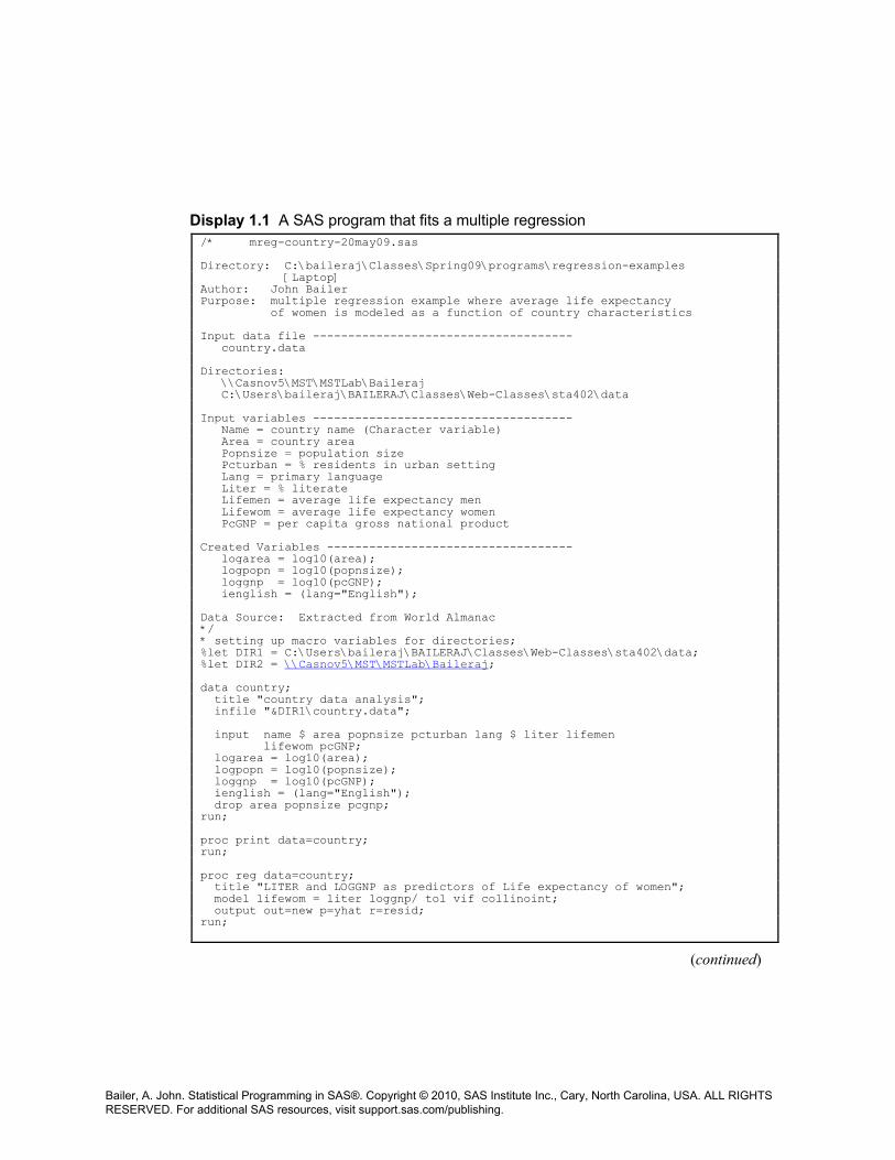
Display 1.1 A SAS program that fits a multiple regression /* mreg-country-20may09.sas Directory: C:\baileraj\Classes\Spring09\programs\regression-examples [Laptop] Author: John Bailer Purpose: multiple regression example where average life expectancy of women is modeled as a function of country characteristics Input data file ------------------------------------- country.data Directories: \\Casnov5\MST\MSTLab\Baileraj C:\Users\baileraj\BAILERAJ\Classes\Web-Classes\sta402\data Input variables ------------------------------------- Name = country name (Character variable) Area = country area Popnsize = population size Pcturban = % residents in urban setting Lang = primary language Liter = % literate Lifemen = average life expectancy men Lifewom = average life expectancy women PcGNP = per capita gross national product Created Variables ----------------------------------- logarea = log10(area); logpopn = log10(popnsize); loggnp = log10(pcGNP); ienglish = (lang="English"); Data Source: Extracted from World Almanac */ * setting up macro variables for directories; %let DIR1 = C:\Users\baileraj\BAILERAJ\Classes\Web-Classes\sta402\data; %let DIR2 = \\Casnov5\MST\MSTLab\Baileraj; data country; title "country data analysis"; infile "&DIR1\country.data"; input name $ area popnsize pcturban lang $ liter lifemen lifewom pcGNP; logarea = log10(area); logpopn = log10(popnsize); loggnp = log10(pcGNP); ienglish = (lang="English"); drop area popnsize pcgnp; run; proc print data=country; run; proc reg data=country; title "LITER and LOGGNP as predictors of Life expectancy of women"; model lifewom = liter loggnp/ tol vif collinoint; output out=new p=yhat r=resid; run;

(continued)



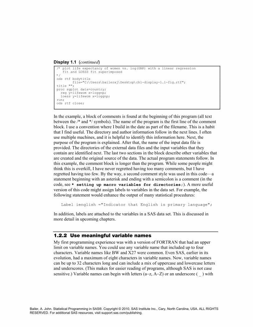
Display 1.1 (continued) /* plot life expectancy of women vs. log(GNP) with a linear regression fit and LOESS fit superimposed */ ods rtf bodytitle file="C:\Users\baileraj\Desktop\ch1-display-1.1-fig.rtf"; title ""; proc sgplot data=country; reg y=lifewom x=loggnp; loess y=lifewom x=loggnp; run; ods rtf close;

In the example, a block of comments is found at the beginning of this program (all text between the /* and */ symbols). The name of the program is the first line of the comment block. I use a convention where I build in the date as part of the filename. This is a habit that I find useful. The directory and author information follow in the next lines. I often use multiple machines, and it is helpful to identify this information here. Next, the purpose of the program is explained. After that, the name of the input data file is provided. The directories of the external data files and the input variables that they contain are identified next. The last two sections in the block describe other variables that are created and the original source of the data. The actual program statements follow. In this example, the comment block is longer than the program. While some people might think this is overkill, I have never regretted having too many comments, but I have regretted having too few. By the way, a second comment style was used in this code—a statement beginning with an asterisk and ending with a semicolon is a comment (in the code, see * setting up macro variables for directories;). A more useful version of this code might assign labels to variables in the data set. For example, the following statement would enhance the output of many statistical procedures:

Label ienglish ="Indicator that English is primary language";

In addition, labels are attached to the variables in a SAS data set. This is discussed in more detail in upcoming chapters.

1.2.2 Use meaningful variable names My first programming experience was with a version of FORTRAN that had an upper limit on variable names. You could use any variable name that included up to four characters. Variable names like BW and X27 were common. Even SAS, earlier in its evolution, had a maximum of eight characters in variable names. Now, variable names can be up to 32 characters long and can include a mix of uppercase and lowercase letters and underscores. (This makes for easier reading of programs, although SAS is not case sensitive.) Variable names can begin with letters (a−z, A−Z) or an underscore ( _ ) with



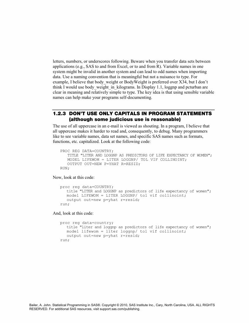
letters, numbers, or underscores following. Beware when you transfer data sets between applications (e.g., SAS to and from Excel, or to and from R). Variable names in one system might be invalid in another system and can lead to odd names when importing data. Use a naming convention that is meaningful but not a nuisance to type. For example, I believe that body_weight or BodyWeight is preferred over X34, but I don’t think I would use body_weight_in_kilograms. In Display 1.1, loggnp and pcturban are clear in meaning and relatively simple to type. The key idea is that using sensible variable names can help make your programs self-documenting.

1.2.3 DON’T USE ONLY CAPITALS IN PROGRAM STATEMENTS (although some judicious use is reasonable) The use of all uppercase in an e-mail is viewed as shouting. In a program, I believe that all uppercase makes it harder to read and, consequently, to debug. Many programmers like to see variable names, data set names, and specific SAS names such as formats, functions, etc. capitalized. Look at the following code:

PROC REG DATA=COUNTRY; TITLE "LITER AND LOGGNP AS PREDICTORS OF LIFE EXPECTANCY OF WOMEN"; MODEL LIFEWOM = LITER LOGGNP/ TOL VIF COLLINOINT; OUTPUT OUT=NEW P=YHAT R=RESID; RUN;

Now, look at this code:

proc reg data=COUNTRY; title "LITER and LOGGNP as predictors of life expectancy of women"; model LIFEWOM = LITER LOGGNP/ tol vif collinoint; output out=new p=yhat r=resid; run;

And, look at this code:

proc reg data=country; title "liter and loggnp as predictors of life expectancy of women"; model lifewom = liter loggnp/ tol vif collinoint; output out=new p=yhat r=resid; run;



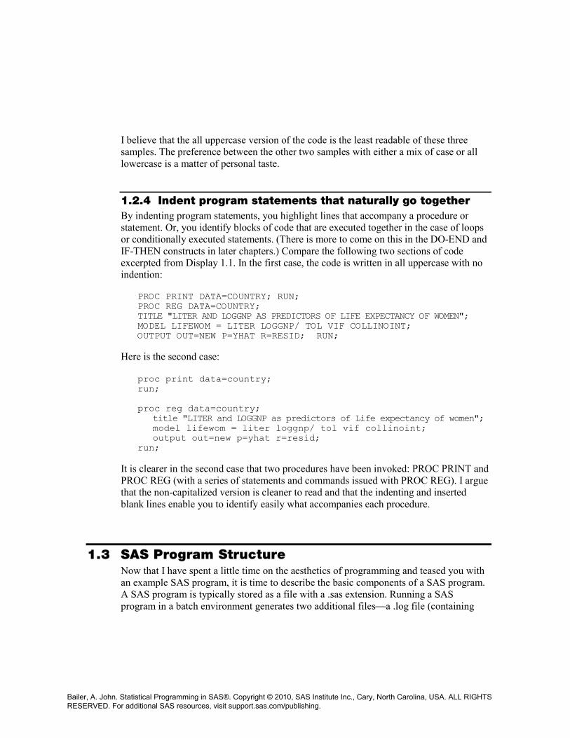
I believe that the all uppercase version of the code is the least readable of these three samples. The preference between the other two samples with either a mix of case or all lowercase is a matter of personal taste.

1.2.4 Indent program statements that naturally go together By indenting program statements, you highlight lines that accompany a procedure or statement. Or, you identify blocks of code that are executed together in the case of loops or conditionally executed statements. (There is more to come on this in the DO-END and IF-THEN constructs in later chapters.) Compare the following two sections of code excerpted from Display 1.1. In the first case, the code is written in all uppercase with no indention:

PROC PRINT DATA=COUNTRY; RUN; PROC REG DATA=COUNTRY; TITLE "LITER AND LOGGNP AS PREDICTORS OF LIFE EXPECTANCY OF WOMEN"; MODEL LIFEWOM = LITER LOGGNP/ TOL VIF COLLINOINT; OUTPUT OUT=NEW P=YHAT R=RESID; RUN;

Here is the second case:

proc print data=country; run; proc reg data=country; title "LITER and LOGGNP as predictors of Life expectancy of women"; model lifewom = liter loggnp/ tol vif collinoint; output out=new p=yhat r=resid; run;

It is clearer in the second case that two procedures have been invoked: PROC PRINT and PROC REG (with a series of statements and commands issued with PROC REG). I argue that the non-capitalized version is cleaner to read and that the indenting and inserted blank lines enable you to identify easily what accompanies each procedure.

1.3 SAS Program Structure Now that I have spent a little time on the aesthetics of programming and teased you with an example SAS program, it is time to describe the basic components of a SAS program. A SAS program is typically stored as a file with a .sas extension. Running a SAS program in a batch environment generates two additional files—a .log file (containing



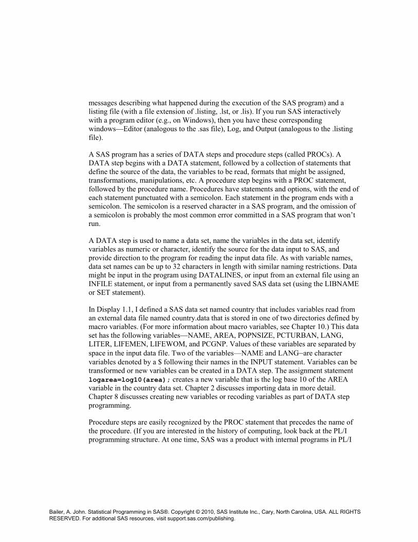
messages describing what happened during the execution of the SAS program) and a listing file (with a file extension of .listing, .lst, or .lis). If you run SAS interactively with a program editor (e.g., on Windows), then you have these corresponding windows—Editor (analogous to the .sas file), Log, and Output (analogous to the .listing file).

A SAS program has a series of DATA steps and procedure steps (called PROCs). A DATA step begins with a DATA statement, followed by a collection of statements that define the source of the data, the variables to be read, formats that might be assigned, transformations, manipulations, etc. A procedure step begins with a PROC statement, followed by the procedure name. Procedures have statements and options, with the end of each statement punctuated with a semicolon. Each statement in the program ends with a semicolon. The semicolon is a reserved character in a SAS program, and the omission of a semicolon is probably the most common error committed in a SAS program that won’t run.

A DATA step is used to name a data set, name the variables in the data set, identify variables as numeric or character, identify the source for the data input to SAS, and provide direction to the program for reading the input data file. As with variable names, data set names can be up to 32 characters in length with similar naming restrictions. Data might be input in the program using DATALINES, or input from an external file using an INFILE statement, or input from a permanently saved SAS data set (using the LIBNAME or SET statement).

In Display 1.1, I defined a SAS data set named country that includes variables read from an external data file named country.data that is stored in one of two directories defined by macro variables. (For more information about macro variables, see Chapter 10.) This data set has the following variables—NAME, AREA, POPNSIZE, PCTURBAN, LANG, LITER, LIFEMEN, LIFEWOM, and PCGNP. Values of these variables are separated by space in the input data file. Two of the variables—NAME and LANG—are character variables denoted by a $ following their names in the INPUT statement. Variables can be transformed or new variables can be created in a DATA step. The assignment statement logarea=log10(area); creates a new variable that is the log base 10 of the AREA variable in the country data set. Chapter 2 discusses importing data in more detail. Chapter 8 discusses creating new variables or recoding variables as part of DATA step programming.

Procedure steps are easily recognized by the PROC statement that precedes the name of the procedure. (If you are interested in the history of computing, look back at the PL/I programming structure. At one time, SAS was a product with internal programs in PL/I



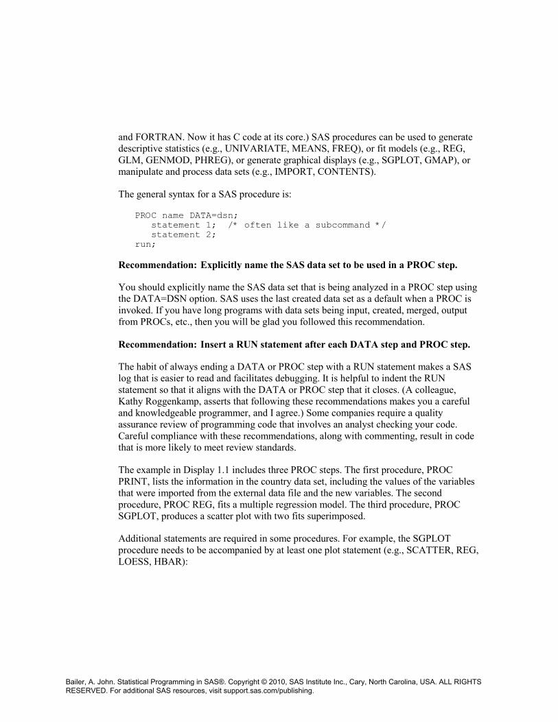
and FORTRAN. Now it has C code at its core.) SAS procedures can be used to generate descriptive statistics (e.g., UNIVARIATE, MEANS, FREQ), or fit models (e.g., REG, GLM, GENMOD, PHREG), or generate graphical displays (e.g., SGPLOT, GMAP), or manipulate and process data sets (e.g., IMPORT, CONTENTS).

The general syntax for a SAS procedure is:

PROC name DATA=dsn; statement 1; /* often like a subcommand */ statement 2; run;

Recommendation: Explicitly name the SAS data set to be used in a PROC step.

You should explicitly name the SAS data set that is being analyzed in a PROC step using the DATA=DSN option. SAS uses the last created data set as a default when a PROC is invoked. If you have long programs with data sets being input, created, merged, output from PROCs, etc., then you will be glad you followed this recommendation.

Recommendation: Insert a RUN statement after each DATA step and PROC step.

The habit of always ending a DATA or PROC step with a RUN statement makes a SAS log that is easier to read and facilitates debugging. It is helpful to indent the RUN statement so that it aligns with the DATA or PROC step that it closes. (A colleague, Kathy Roggenkamp, asserts that following these recommendations makes you a careful and knowledgeable programmer, and I agree.) Some companies require a quality assurance review of programming code that involves an analyst checking your code. Careful compliance with these recommendations, along with commenting, result in code that is more likely to meet review standards.

The example in Display 1.1 includes three PROC steps. The first procedure, PROC PRINT, lists the information in the country data set, including the values of the variables that were imported from the external data file and the new variables. The second procedure, PROC REG, fits a multiple regression model. The third procedure, PROC SGPLOT, produces a scatter plot with two fits superimposed.

Additional statements are required in some procedures. For example, the SGPLOT procedure needs to be accompanied by at least one plot statement (e.g., SCATTER, REG, LOESS, HBAR):



ods rtf bodytitle file="C:\Users\baileraj\Desktop\ch1-display-1.1-fig.rtf"; proc sgplot data=country; reg y=lifewom x=loggnp; loess y=lifewom x=loggnp; run; ods rtf close;

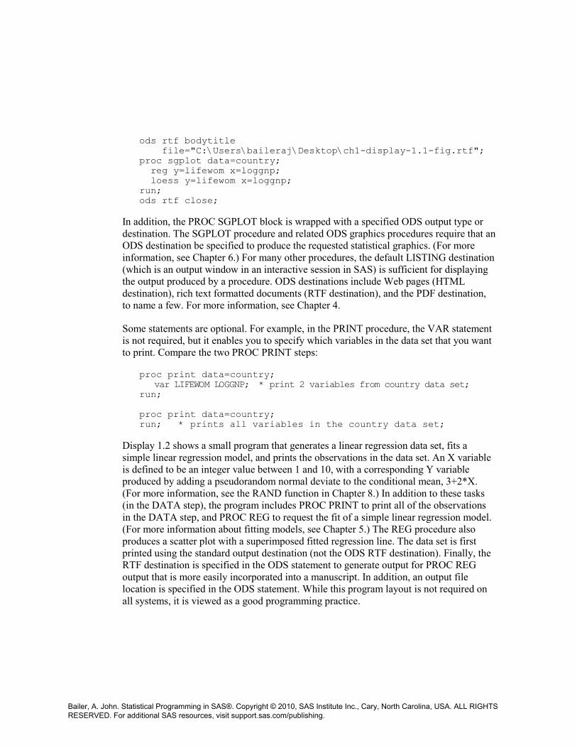
In addition, the PROC SGPLOT block is wrapped with a specified ODS output type or destination. The SGPLOT procedure and related ODS graphics procedures require that an ODS destination be specified to produce the requested statistical graphics. (For more information, see Chapter 6.) For many other procedures, the default LISTING destination (which is an output window in an interactive session in SAS) is sufficient for displaying the output produced by a procedure. ODS destinations include Web pages (HTML destination), rich text formatted documents (RTF destination), and the PDF destination, to name a few. For more information, see Chapter 4.

Some statements are optional. For example, in the PRINT procedure, the VAR statement is not required, but it enables you to specify which variables in the data set that you want to print. Compare the two PROC PRINT steps:

proc print data=country; var LIFEWOM LOGGNP; * print 2 variables from country data set; run; proc print data=country; run; * prints all variables in the country data set;

Display 1.2 shows a small program that generates a linear regression data set, fits a simple linear regression model, and prints the observations in the data set. An X variable is defined to be an integer value between 1 and 10, with a corresponding Y variable produced by adding a pseudorandom normal deviate to the conditional mean, 3+2*X. (For more information, see the RAND function in Chapter 8.) In addition to these tasks (in the DATA step), the program includes PROC PRINT to print all of the observations in the DATA step, and PROC REG to request the fit of a simple linear regression model. (For more information about fitting models, see Chapter 5.) The REG procedure also produces a scatter plot with a superimposed fitted regression line. The data set is first printed using the standard output destination (not the ODS RTF destination). Finally, the RTF destination is specified in the ODS statement to generate output for PROC REG output that is more easily incorporated into a manuscript. In addition, an output file location is specified in the ODS statement. While this program layout is not required on all systems, it is viewed as a good programming practice.



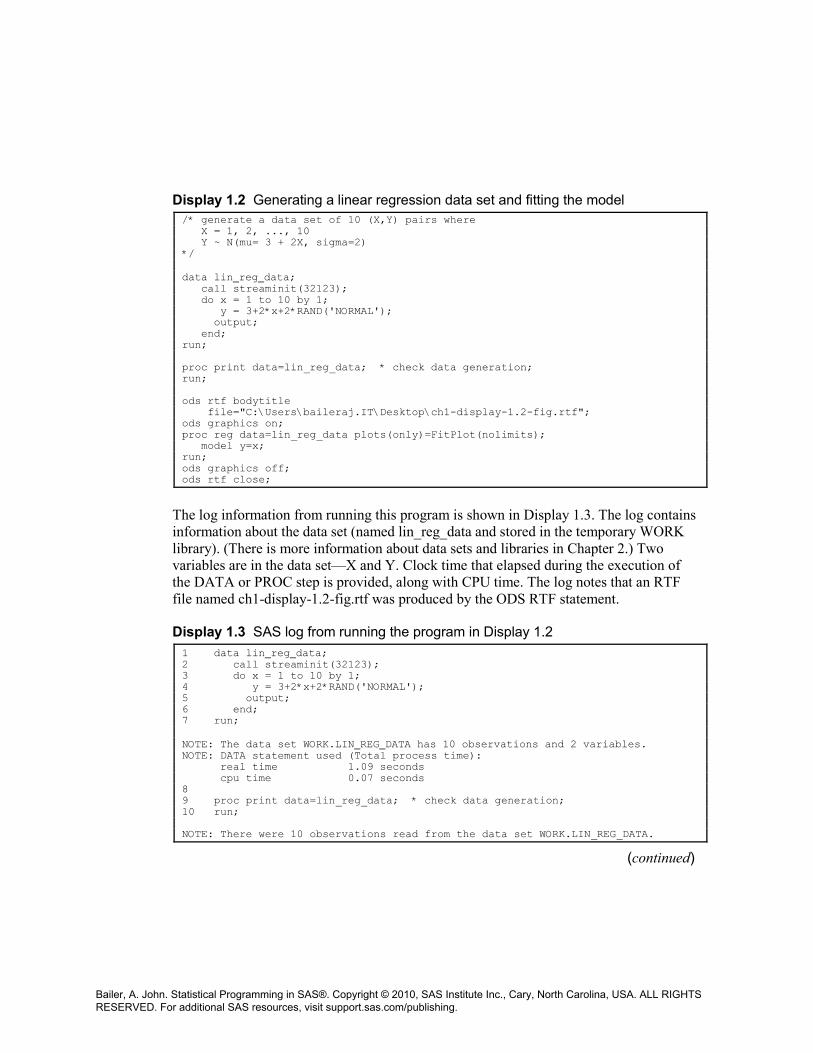
Display 1.2 Generating a linear regression data set and fitting the model /* generate a data set of 10 (X,Y) pairs where X = 1, 2, ..., 10 Y ~ N(mu= 3 + 2X, sigma=2) */ data lin_reg_data; call streaminit(32123); do x = 1 to 10 by 1; y = 3+2*x+2*RAND('NORMAL'); output; end; run; proc print data=lin_reg_data; * check data generation; run; ods rtf bodytitle file="C:\Users\baileraj.IT\Desktop\ch1-display-1.2-fig.rtf"; ods graphics on; proc reg data=lin_reg_data plots(only)=FitPlot(nolimits); model y=x; run; ods graphics off; ods rtf close;

The log information from running this program is shown in Display 1.3. The log contains information about the data set (named lin_reg_data and stored in the temporary WORK library). (There is more information about data sets and libraries in Chapter 2.) Two variables are in the data set—X and Y. Clock time that elapsed during the execution of the DATA or PROC step is provided, along with CPU time. The log notes that an RTF file named ch1-display-1.2-fig.rtf was produced by the ODS RTF statement.

Display 1.3 SAS log from running the program in Display 1.2 1 data lin_reg_data; 2 call streaminit(32123); 3 do x = 1 to 10 by 1; 4 y = 3+2*x+2*RAND('NORMAL'); 5 output; 6 end; 7 run; NOTE: The data set WORK.LIN_REG_DATA has 10 observations and 2 variables. NOTE: DATA statement used (Total process time): real time 1.09 seconds cpu time 0.07 seconds 8 9 proc print data=lin_reg_data; * check data generation; 10 run; NOTE: There were 10 observations read from the data set WORK.LIN_REG_DATA.

(continued)



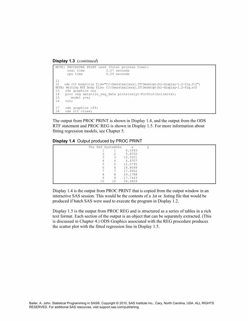
Display 1.3 (continued) NOTE: PROCEDURE PRINT used (Total process time): real time 2.27 seconds cpu time 0.29 seconds 11 12 ods rtf bodytitle file="C:\Users\baileraj.IT\Desktop\ch1-display-1.2-fig.rtf"; NOTE: Writing RTF Body file: C:\Users\baileraj.IT\Desktop\ch1-display-1.2-fig.rtf 13 ods graphics on; 14 proc reg data=lin_reg_data plots(only)=FitPlot(nolimits); 15 model y=x; 16 run; 17 ods graphics off; 18 ods rtf close;

The output from PROC PRINT is shown in Display 1.4, and the output from the ODS RTF statement and PROC REG is shown in Display 1.5. For more information about fitting regression models, see Chapter 5.

Display 1.4 Output produced by PROC PRINT The SAS SystemObs x y 1 1 6.1693 2 2 5.8702 3 3 10.5551 4 4 6.9707 5 5 12.0795 6 6 14.8699 7 7 17.9952 8 8 19.1788 9 9 17.7443 10 10 24.5809

Display 1.4 is the output from PROC PRINT that is copied from the output window in an interactive SAS session. This would be the contents of a .lst or .listing file that would be produced if batch SAS were used to execute the program in Display 1.2.

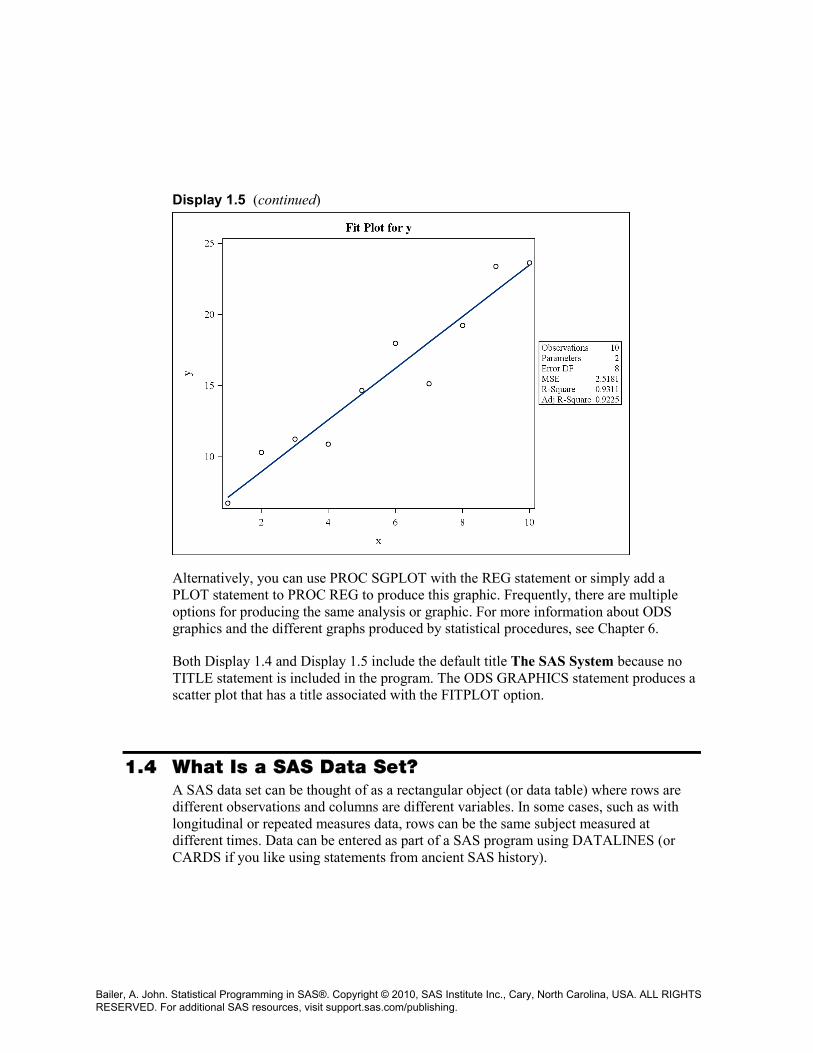
Display 1.5 is the output from PROC REG and is structured as a series of tables in a rich text format. Each section of the output is an object that can be separately extracted. (This is discussed in Chapter 4.) ODS Graphics associated with the REG procedure produces the scatter plot with the fitted regression line in Display 1.5.



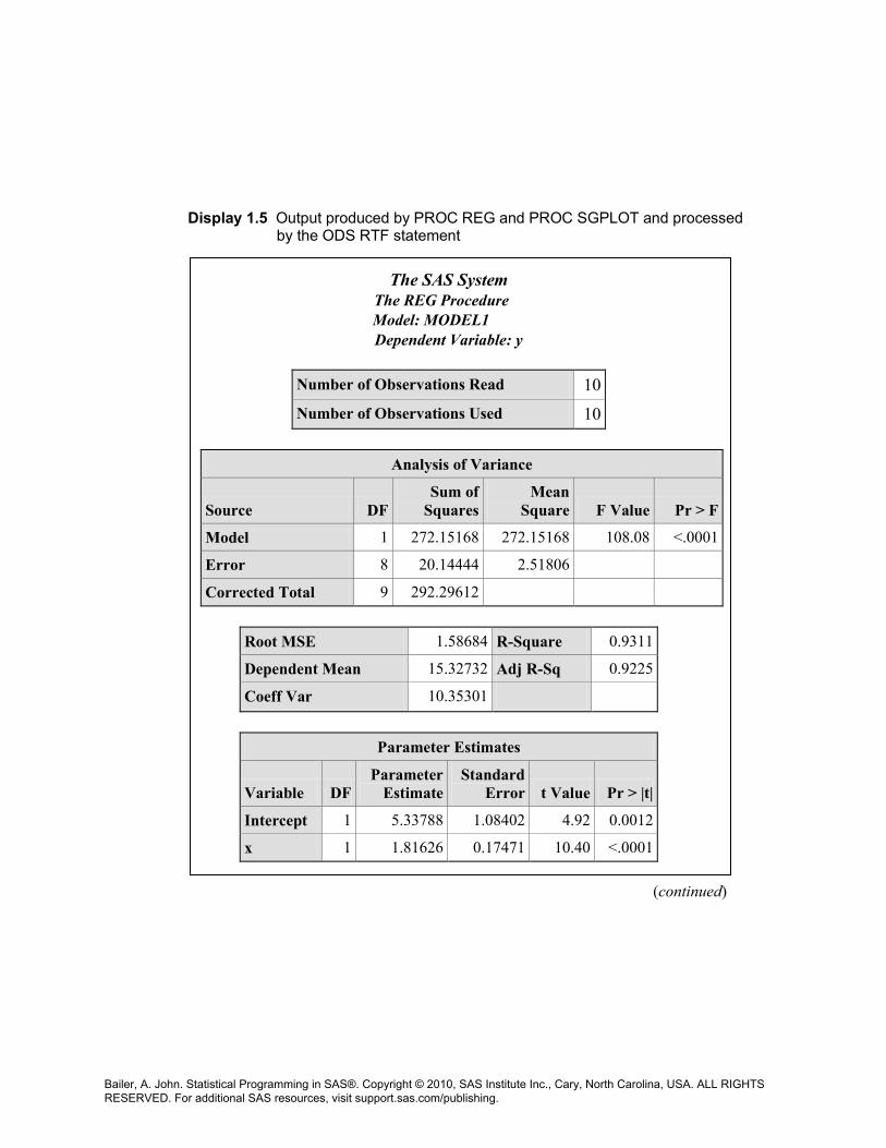
Display 1.5 Output produced by PROC REG and PROC SGPLOT and processed by the ODS RTF statement

The SAS System

The REG Procedure Model: MODEL1 Dependent Variable: y

Number of Observations Read 10 Number of Observations Used 10

Analysis of Variance

Source DF Sum of

Squares Mean

Square F Value Pr > F

Model 1 272.15168 272.15168 108.08 <.0001

Error 8 20.14444 2.51806

Corrected Total 9 292.29612

Root MSE 1.58684 R-Square 0.9311

Dependent Mean 15.32732 Adj R-Sq 0.9225

Coeff Var 10.35301

Parameter Estimates

Variable DF Parameter

Estimate Standard

Error t Value Pr > |t|

Intercept 1 5.33788 1.08402 4.92 0.0012

x 1 1.81626 0.17471 10.40 <.0001 (continued)



Display 1.5 (continued)

Alternatively, you can use PROC SGPLOT with the REG statement or simply add a PLOT statement to PROC REG to produce this graphic. Frequently, there are multiple options for producing the same analysis or graphic. For more information about ODS graphics and the different graphs produced by statistical procedures, see Chapter 6.

Both Display 1.4 and Display 1.5 include the default title The SAS System because no TITLE statement is included in the program. The ODS GRAPHICS statement produces a scatter plot that has a title associated with the FITPLOT option.

1.4 What Is a SAS Data Set? A SAS data set can be thought of as a rectangular object (or data table) where rows are different observations and columns are different variables. In some cases, such as with longitudinal or repeated measures data, rows can be the same subject measured at different times. Data can be entered as part of a SAS program using DATALINES (or CARDS if you like using statements from ancient SAS history).



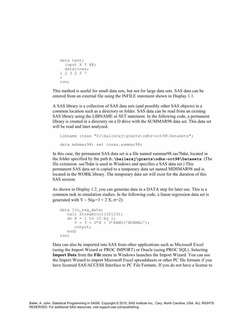
data test; input X Y @@; datalines; 1 2 3 2 5 7 ; run;

This method is useful for small data sets, but not for large data sets. SAS data can be entered from an external file using the INFILE statement shown in Display 1.1.

A SAS library is a collection of SAS data sets (and possibly other SAS objects) in a common location such as a directory or folder. SAS data can be read from an existing SAS library using the LIBNAME or SET statement. In the following code, a permanent library is created in a directory on a D drive with the SUMMAR98 data set. This data set will be read and later analyzed.

Libname insas "D:\baileraj\grants\odhs-oct98\Datasets"; data mdsmar98; set insas.summar98;

In this case, the permanent SAS data set is a file named summar98.sas7bdat, located in the folder specified by the path D:\baileraj\grants\odhs-oct98\Datasets. (The file extension .sas7bdat is used in Windows and specifies a SAS data set.) This permanent SAS data set is copied to a temporary data set named MDSMAR98 and is located in the WORK library. The temporary data set will exist for the duration of this SAS session.

As shown in Display 1.2, you can generate data in a DATA step for later use. This is a common task in simulation studies. In the following code, a linear regression data set is generated with Y ~ N(µ=3 + 2 X, σ=2):

data lin_reg_data; call streaminit(32123); do X = 1 to 10 by 1; Y = 3 + 2*X + 2*RAND('NORMAL'); output; end; run;

Data can also be imported into SAS from other applications such as Microsoft Excel (using the Import Wizard or PROC IMPORT) or Oracle (using PROC SQL). Selecting Import Data from the File menu in Windows launches the Import Wizard. You can use the Import Wizard to import Microsoft Excel spreadsheets or other PC file formats if you have licensed SAS/ACCESS Interface to PC File Formats. If you do not have a license to



use this software, then the Import Wizard can still be used to import text files or comma-separated, tab-delimited, or any type of delimited files. For more information about importing data from external sources and manipulating it to build an analysis data set, see Chapter 2.

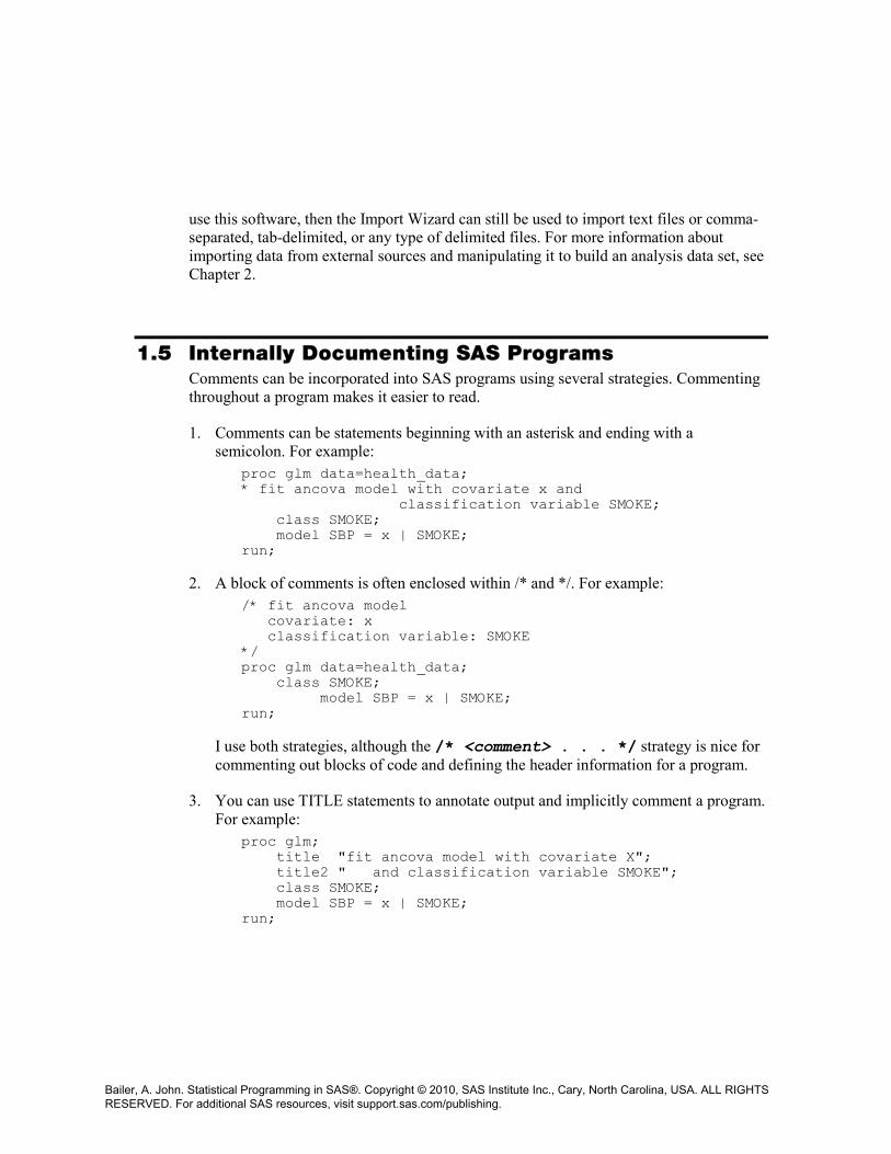
1.5 Internally Documenting SAS Programs Comments can be incorporated into SAS programs using several strategies. Commenting throughout a program makes it easier to read.

1. Comments can be statements beginning with an asterisk and ending with a semicolon. For example: proc glm data=health_data; * fit ancova model with covariate x and classification variable SMOKE; class SMOKE; model SBP = x | SMOKE; run;

2. A block of comments is often enclosed within /* and */. For example: /* fit ancova model covariate: x classification variable: SMOKE */ proc glm data=health_data; class SMOKE; model SBP = x | SMOKE; run; I use both strategies, although the /* <comment> . . . */ strategy is nice for commenting out blocks of code and defining the header information for a program.

3. You can use TITLE statements to annotate output and implicitly comment a program. For example: proc glm; title "fit ancova model with covariate X"; title2 " and classification variable SMOKE"; class SMOKE; model SBP = x | SMOKE; run;



1.6 Summary This chapter provides an introduction to SAS. But, more important, it suggests coding habits for structuring and documenting a program to make it easier to read, debug, maintain, and modify. In the chapters that follow, the use of SAS to address data analytic problems is discussed in detail. Chapter 2 discusses creating an analysis data set, which typically involves reading an external data source into SAS, and then processing the data set. Chapter 3 presents basic descriptive and graphical statistics, which is followed by creating fancier, more customized tables and output in Chapter 4. The first section of the book concludes with chapters addressing the specifications of statistical models in SAS, and the production of statistical graphics.

1.7 References Allison, T., and D. Cicchetti “Sleep in Mammals: Ecological and Constitutional

Correlates.” Science 194 (1976): No. 4266, pp. 732−734. Cody, Ronald, and Ray Pass. 1995. SAS Programming by Example. Cary, NC: SAS

Institute Inc. Delwiche, Lora D., and Susan J. Slaughter. 2008. The Little SAS Book: A Primer, Fourth

Edition. Cary, NC: SAS Institute Inc. Givens, Geof H., and Jennifer A. Hoeting. 2005. Computational Statistics. Hoboken, NJ:

Wiley Interscience. Moore, David S., and George P. McCabe. 2003. Introduction to the Practice of Statistics.

4th Ed. New York: NY: W. H. Freeman and Co.

1.8 Exercises 1. In the following code, Y=year, X=number of boats registered (in multiples of 1000),

and Z=number of manatees killed.1

Modify this program to make it more readable. Add an introductory comment block to describe this program.

1 Manatee data set usage based on “Florida powerboats and manatee deaths, 1977–1990” data set from Moore, David S., and George P. McCabe. 2003. Introduction to the Practice of Statistics. 4th Ed. New York, NY: W. H. Freeman and Co.



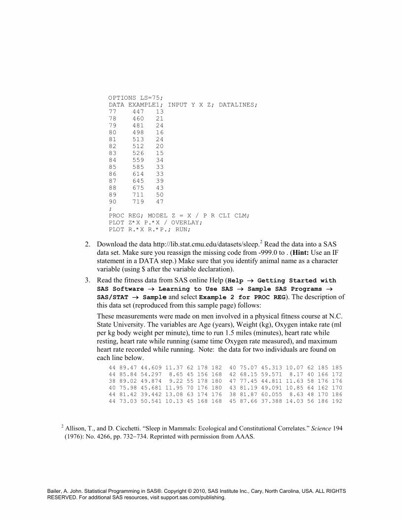
OPTIONS LS=75; DATA EXAMPLE1; INPUT Y X Z; DATALINES; 77 447 13 78 460 21 79 481 24 80 498 16 81 513 24 82 512 20 83 526 15 84 559 34 85 585 33 86 614 33 87 645 39 88 675 43 89 711 50 90 719 47 ; PROC REG; MODEL Z = X / P R CLI CLM; PLOT Z*X P.*X / OVERLAY; PLOT R.*X R.*P.; RUN;

2. Download the data http://lib.stat.cmu.edu/datasets/sleep.2

3. Read the fitness data from SAS online Help (Help → Getting Started with SAS Software → Learning to Use SAS → Sample SAS Programs → SAS/STAT → Sample and select Example 2 for PROC REG). The description of this data set (reproduced from this sample page) follows:

Read the data into a SAS data set. Make sure you reassign the missing code from -999.0 to . (Hint: Use an IF statement in a DATA step.) Make sure that you identify animal name as a character variable (using $ after the variable declaration).

These measurements were made on men involved in a physical fitness course at N.C. State University. The variables are Age (years), Weight (kg), Oxygen intake rate (ml per kg body weight per minute), time to run 1.5 miles (minutes), heart rate while resting, heart rate while running (same time Oxygen rate measured), and maximum heart rate recorded while running. Note: the data for two individuals are found on each line below.

44 89.47 44.609 11.37 62 178 182 40 75.07 45.313 10.07 62 185 185 44 85.84 54.297 8.65 45 156 168 42 68.15 59.571 8.17 40 166 172 38 89.02 49.874 9.22 55 178 180 47 77.45 44.811 11.63 58 176 176 40 75.98 45.681 11.95 70 176 180 43 81.19 49.091 10.85 64 162 170 44 81.42 39.442 13.08 63 174 176 38 81.87 60.055 8.63 48 170 186 44 73.03 50.541 10.13 45 168 168 45 87.66 37.388 14.03 56 186 192

2 Allison, T., and D. Cicchetti. “Sleep in Mammals: Ecological and Constitutional Correlates.” Science 194 (1976): No. 4266, pp. 732−734. Reprinted with permission from AAAS.


http://lib.stat.cmu.edu/datasets/sleep�


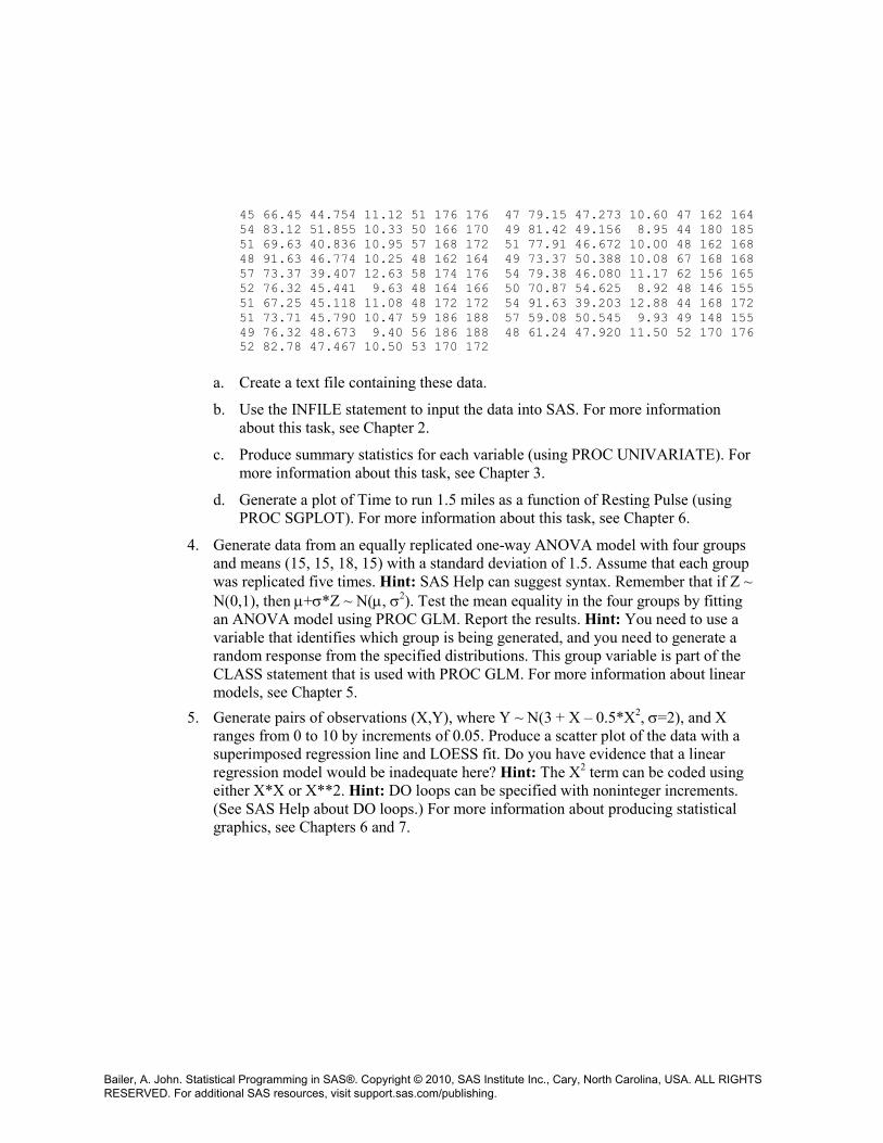
45 66.45 44.754 11.12 51 176 176 47 79.15 47.273 10.60 47 162 164 54 83.12 51.855 10.33 50 166 170 49 81.42 49.156 8.95 44 180 185 51 69.63 40.836 10.95 57 168 172 51 77.91 46.672 10.00 48 162 168 48 91.63 46.774 10.25 48 162 164 49 73.37 50.388 10.08 67 168 168 57 73.37 39.407 12.63 58 174 176 54 79.38 46.080 11.17 62 156 165 52 76.32 45.441 9.63 48 164 166 50 70.87 54.625 8.92 48 146 155 51 67.25 45.118 11.08 48 172 172 54 91.63 39.203 12.88 44 168 172 51 73.71 45.790 10.47 59 186 188 57 59.08 50.545 9.93 49 148 155 49 76.32 48.673 9.40 56 186 188 48 61.24 47.920 11.50 52 170 176 52 82.78 47.467 10.50 53 170 172

a. Create a text file containing these data.

b. Use the INFILE statement to input the data into SAS. For more information about this task, see Chapter 2.

c. Produce summary statistics for each variable (using PROC UNIVARIATE). For more information about this task, see Chapter 3.

d. Generate a plot of Time to run 1.5 miles as a function of Resting Pulse (using PROC SGPLOT). For more information about this task, see Chapter 6.

4. Generate data from an equally replicated one-way ANOVA model with four groups and means (15, 15, 18, 15) with a standard deviation of 1.5. Assume that each group was replicated five times. Hint: SAS Help can suggest syntax. Remember that if Z ~ N(0,1), then µ+σ*Z ~ N(µ, σ2). Test the mean equality in the four groups by fitting an ANOVA model using PROC GLM. Report the results. Hint: You need to use a variable that identifies which group is being generated, and you need to generate a random response from the specified distributions. This group variable is part of the CLASS statement that is used with PROC GLM. For more information about linear models, see Chapter 5.

5. Generate pairs of observations (X,Y), where Y ~ N(3 + X – 0.5*X2, σ=2), and X ranges from 0 to 10 by increments of 0.05. Produce a scatter plot of the data with a superimposed regression line and LOESS fit. Do you have evidence that a linear regression model would be inadequate here? Hint: The X2 term can be coded using either X*X or X**2. Hint: DO loops can be specified with noninteger increments. (See SAS Help about DO loops.) For more information about producing statistical graphics, see Chapters 6 and 7.





Documents

Part - Analytics, Business Intelligence and Data … 1 Let's Get Started—Preliminaries and a SAS Quick Start..... 3 Chapter 2 Reading, Combining, and Managing Data for Later Analysis