PART I: INTRODUCTION

Radiation and Matter

Section 1

Radiation

Almost all the astrophysical information we can derive about distant sources results from the

radiation that reaches us from them. Our starting point is, therefore, a review of the principal

ways of describing radiation. (In principle, this could include polarization properties, but we

neglect that for simplicity).

The fundamental denitions of interest are of (specic) intensity and (physical) ux.

1.1 Specic Intensity, Iν

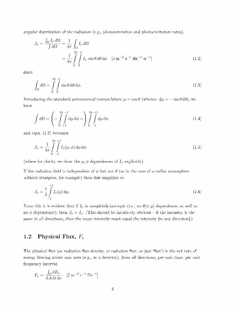
The specic intensity (or radiation intensity, or surface brightness) is dened as:

the rate of energy owing at a given point,

per unit area,

per unit time,

per unit frequency interval,

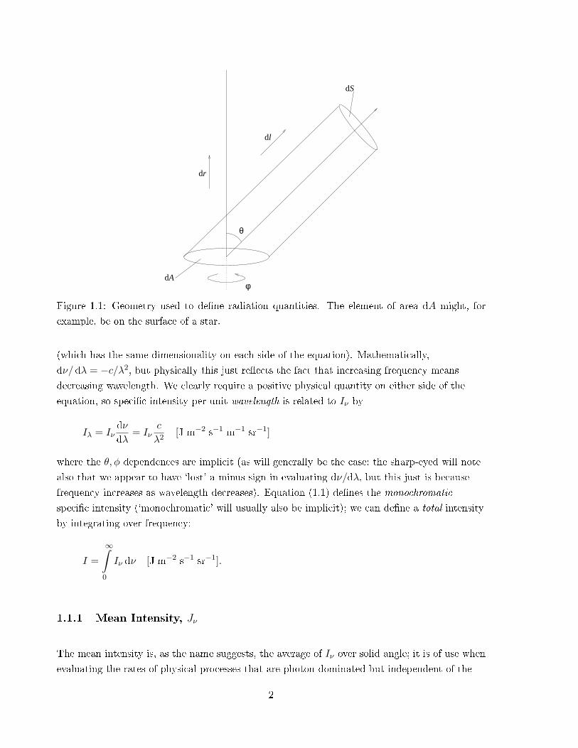
per unit solid angle (in azimuth φ and direction θ to the normal; refer to the

geometry sketched in Fig. 1.1)

or, expressed algebraically,

Iν(θ, φ) =dEν

dS dt dν dΩ

=dEν

dA cos θ dt dν dΩ[J m−2 s−1 Hz−1 sr−1]. (1.1)

We've given a `per unit frequency denition', but we can always switch to `per unit wavelength'

by noting that, for some frequency-dependent physical quantity ‘X', we can write

Xν dν = Xλ dλ.

1

dA

dr

dl

dS

φ

θ

Figure 1.1: Geometry used to dene radiation quantities. The element of area dA might, for

example, be on the surface of a star.

(which has the same dimensionality on each side of the equation). Mathematically,

dν/ dλ = −c/λ2, but physically this just reects the fact that increasing frequency means

decreasing wavelength. We clearly require a positive physical quantity on either side of the

equation, so specic intensity per unit wavelength is related to Iν by

Iλ = Iνdνdλ

= Iνc

λ2[J m−2 s−1 m−1 sr−1]

where the θ, φ dependences are implicit (as will generally be the case; the sharp-eyed will note

also that we appear to have `lost' a minus sign in evaluating dν/dλ, but this just is because

frequency increases as wavelength decreases). Equation (1.1) denes the monochromatic

specic intensity (`monochromatic' will usually also be implicit); we can dene a total intensity

by integrating over frequency:

I =

∞∫0

Iν dν [J m−2 s−1 sr−1].

1.1.1 Mean Intensity, Jν

The mean intensity is, as the name suggests, the average of Iν over solid angle; it is of use when

evaluating the rates of physical processes that are photon dominated but independent of the

2

angular distribution of the radiation (e.g., photoionization and photoexcitation rates).

Jν =

∫Ω Iν dΩ∫

dΩ=

14π

∫Ω

Iν dΩ

=14π

2π∫0

π∫0

Iν sin θ dθ dφ [J m−2 s−1 Hz−1 sr−1] (1.2)

since ∫Ω

dΩ =

2π∫0

π∫0

sin θ dθ dφ. (1.3)

Introducing the standard astronomical nomenclature µ = cos θ (whence dµ = − sin θ dθ), we

have ∫dΩ =

− 2π∫0

−1∫+1

dµ dφ =

2π∫0

+1∫−1

dµ dφ (1.4)

and eqtn. (1.2) becomes

Jν =14π

2π∫0

+1∫−1

Iν(µ, φ) dµ dφ (1.5)

(where for clarity we show the µ, φ dependences of Iν explicitly).

If the radiation eld is independent of φ but not θ (as in the case of a stellar atmosphere

without starspots, for example) then this simplies to

Jν =12

+1∫−1

Iν(µ) dµ. (1.6)

From this it is evident that if Iν is completely isotropic (i.e., no θ[≡ µ] dependence, as well asno φ dependence), then Jν = Iν . (This should be intuitively obvious if the intensity is the

same in all directions, then the mean intensity must equal the intensity [in any direction].)

1.2 Physical Flux, Fν

The physical ux (or radiation ux density, or radiation ux, or just `ux') is the net rate of

energy owing across unit area (e.g., at a detector), from all directions, per unit time, per unit

frequency interval:

Fν =

∫Ω dEν

dA dt dν[J m−2 s−1 Hz−1]

3

It is the absence of directionality that crucially distinguishes ux from intensity, but the two

are clearly related. Using eqtn. (1.1) we see that

Fν =∫

ΩIν cos θ dΩ (1.7)

=

2π∫0

π∫0

Iν cos θ sin θ dθ dφ [J m−2 Hz−1] (1.8)

=

2π∫0

+1∫−1

Iν(µ, φ)µ dµ dφ

or, if there is no φ dependence,

Fν = 2π

+1∫−1

Iν(µ)µ dµ. (1.9)

Because we're simply measuring the energy owing across an area, there's no explicit

directionality involved other than if the energy impinges on the area from `above' or `below'.1

It's therefore often convenient to divide the contributions to the ux into the `upward'

(emitted, or `outward') radiation (F+ν ; 0 ≤ θ ≤ π/2, Fig 1.1) and the `downward' (incident, or

`inward') radiation (F−ν ;π/2 ≤ θ ≤ π), with the net upward ux being Fν = F+

ν − F−ν :

Fν =

2π∫0

π/2∫0

Iν cos θ sin θ dθ dφ +

2π∫0

π∫π/2

Iν cos θ sin θ dθ dφ

≡ F+ν − F−

ν

As an important example, the surface ux emitted by a star is just F+ν (assuming there is no

incident external radiation eld);

Fν = F+ν =

2π∫0

π/2∫0

Iν cos θ sin θ dθ dφ

or, if there is no φ dependence,

= 2π

π/2∫0

Iν cos θ sin θ dθ.

= 2π

+1∫0

Iν(µ)µ dµ. (1.10)

1In principle, ux is a vector quantity, but the directionality is almost always implicit in astrophysical situations;

e.g., from the centre of a star outwards, or from a source to an observer.

4

If, furthermore, Iν has no θ dependence over the range 0π/2 then

Fν = πIν (1.11)

(since∫ π/20 cos θ sin θ dθ = 1/2). If Iν is completely isotropic, then F+

ν = F−ν , and Fν = 0.

1.3 Flux vs. Intensity

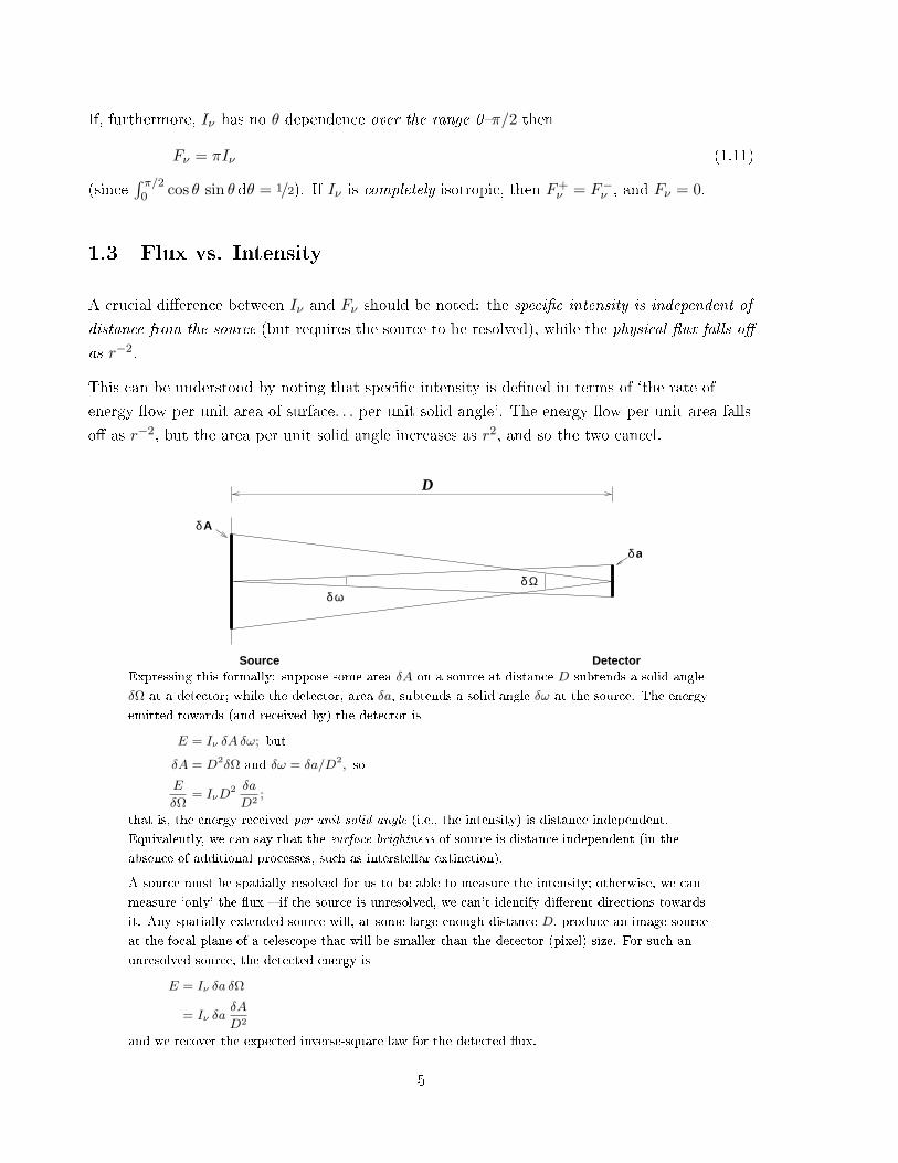
A crucial dierence between Iν and Fν should be noted: the specic intensity is independent of

distance from the source (but requires the source to be resolved), while the physical ux falls o

as r−2.

This can be understood by noting that specic intensity is dened in terms of `the rate of

energy ow per unit area of surface. . . per unit solid angle'. The energy ow per unit area falls

o as r−2, but the area per unit solid angle increases as r2, and so the two cancel.

δA

δa

δ ωδ Ω

DetectorSource

D

Expressing this formally: suppose some area δA on a source at distance D subtends a solid angle

δΩ at a detector; while the detector, area δa, subtends a solid angle δω at the source. The energy

emitted towards (and received by) the detector is

E = Iν δA δω; but

δA = D2δΩ and δω = δa/D2, so

E

δΩ= IνD

2 δa

D2;

that is, the energy received per unit solid angle (i.e., the intensity) is distance independent.

Equivalently, we can say that the surface brightness of source is distance independent (in the

absence of additional processes, such as interstellar extinction).

A source must be spatially resolved for us to be able to measure the intensity; otherwise, we can

measure `only' the ux if the source is unresolved, we can't identify dierent directions towards

it. Any spatially extended source will, at some large enough distance D, produce an image source

at the focal plane of a telescope that will be smaller than the detector (pixel) size. For such an

unresolved source, the detected energy is

E = Iν δa δΩ

= Iν δaδA

D2

and we recover the expected inverse-square law for the detected ux.

5

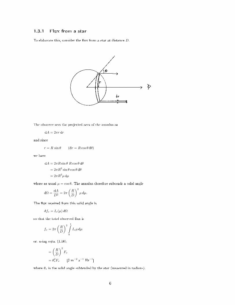
1.3.1 Flux from a star

To elaborate this, consider the ux from a star at distance D.

The observer sees the projected area of the annulus as

dA = 2πr dr

and since

r = R sin θ (dr = R cos θ dθ)

we have

dA = 2πR sin θ R cos θ dθ

= 2πR2 sin θ cos θ dθ

= 2πR2µ dµ

where as usual µ = cos θ. The annulus therefore subtends a solid angle

dΩ =dA

D2= 2π

„R

D

«2

µ dµ.

The ux received from this solid angle is

dfν = Iν(µ)dΩ

so that the total observed ux is

fν = 2π

„R

D

«21Z

0

Iνµ dµ

or, using eqtn. (1.10),

=

„R

D

«2

Fν

= θ2∗Fν [J m−2 s−1 Hz−1]

where θ∗ is the solid angle subtended by the star (measured in radians).

6

1.4 Flux Moments

Flux moments are a traditional `radiation' topic, of use in studying the transport of radiation

in stellar atmospheres. The nth moment of the radiation eld is dened as

Mν ≡12

+1∫−1

Iν(µ)µn dµ. (1.12)

We can see that we've already encountered the zeroth-order moment, which is the mean

intensity:

Jν =12

+1∫−1

Iν(µ) dµ. (1.6)

We have previously written the ux as

Fν = 2π

+1∫−1

Iν(µ)µ dµ; (1.9)

to cast this in the same form as eqtns. (1.12) and (1.6), we dene the `Eddington ux' as

Hν = Fν/(4π), i.e.,

Hν =12

∫ +1

−1Iν(µ)µ dµ. (1.13)

We see that Hν is the rst-order moment of the radiation eld.

The second-order moment, the so-called ‘K integral', is, from the denition of moments,

Kν =12

+1∫−1

Iν(µ)µ2 dµ (1.14)

In the special case that Iν is isotropic we can take it out of the integration over µ, and

Kν =12

µ3

3Iν

∣∣∣∣+1

−1

=13Iν

[also =

13Jν for isotropy

](1.15)

We will see in Section 1.8 that the K integral is straightforwardly related to radiation pressure.

Higher-order moments are rarely used. So, to recap (and using the notation rst introduced by

Eddington himself), for n = 0, 1, 2:n = 0 Mean Intensity Jν = 1

2

∫ +1−1 Iν(µ) dµ

n = 1 Eddington ux Hν = 12

∫ +1−1 Iν(µ)µ dµ

n = 2 K integral Kν = 12

∫ +1−1 Iν(µ)µ2 dµ

7

(all with units [J m−2 s−1 Hz−1 sr−1]).

We can also dene the integral quantities

J =∫ ∞

0Jν dν

F =∫ ∞

0Fν dν

K =∫ ∞

0Kν dν

1.5 Other `Fluxes', `Intensities'

Astronomers can be rather careless in their use of the terms `ux'. and `intensity'. The `uxes'

and `intensities' discussed so far can all be quantied in terms of physical (e.g., SI) units.

Often, however, astronomical signals are measured in more arbitrary ways (such `integrated

signal at the detector', or even `photographic density'); in such cases, it's commonplace to refer

to the `intensity' in a spectrum, but this is just a loose shorthand, and doesn't allude to the

true specic intensity dened in this section.

There are other physically-based quantities that one should be aware of. For example,

discussions of model stellar atmospheres may refer to the `astrophysical ux'; this is given by

Fν/π (also called, rarely, the `radiative ux'), which is evidently similar to the Eddington ux,

Hν = Fν/(4π), which has itself also occasionally been referred to as the `Harvard ux'.

Confusingly, some authors also call it just `the ux', but it's always written as Hν (never Fν).

1.6 Black-body radiation (reference/revision only)

In astrophysics, a radiation eld can often be usefully approximated by that of a `black body', for

which the intensity is given by the Planck function:

Iν = Bν(T ) =2hν3

c2

exp

„hν

kT

«− 1

ff−1

[J m−2 s−1 Hz−1 sr−1]; or (1.16)

Iλ = Bλ(T ) =2hc2

λ5

exp

„hc

λkT

«− 1

ff−1

[J m−2 s−1 m−1 sr−1] (1.17)

(where Bν dν = Bλ dλ).

We have seen that

Fν = 2π

+1Z−1

Iν(µ)µ dµ. (1.9)

8

If we have a surface radiating like a black body then Iν = Bν(T ), and there is no µ dependence,

other than that the energy is emitted over the limits 0 ≤ µ ≤ 1; thus the physical ux for a

black-body radiator is given by

Fν = F+ν = 2π

+1Z0

Bν(T )µ dµ = Bν2πµ2

2

˛+1

0

= πBν . (1.18)

(cp. eqtn. (1.11): Fν = πIν)

1.6.1 Integrated ux

The total radiant energy ux is obtained by integrating eqtn. (1.18) over frequency,Z ∞

0

Fν dν =

Z ∞

0

πBν dν

=

Z ∞

0

2πhν3

c2

exp

„hν

kT

«− 1

ff−1

dν. (1.19)

We can solve this by setting x = (hν)/(kT ) (whence dν = [kT/h] dx), soZ ∞

0

Fν dν =

„kT

h

«42πh

c2

Z ∞

0

x3

exp(x)− 1dx

The integral is now a standard form, which has the solution π4/15, whenceZ ∞

0

Fν dν =

„kπ

h

«42πh

15c2T 4 (1.20)

≡ σT 4 (1.21)

where σ is the Stefan-Boltzmann constant,

σ =2π5k4

15h3c2= 5.67× 10−5 [J m−2 K−4 s−1].

1.6.2 Approximate forms

There are two important approximations to the Planck function which follow directly from

eqtn. 1.16:

Bν(T ) ' 2hν3

c2

exp

„hν

kT

«ff−1

forhν

kT 1 (1.22)

(Wien approximation), and

Bν(T ) ' 2ν2kT

c2for

hν

kT 1 (1.23)

(Rayleigh-Jeans approximation; exp(hν/kT ) ' 1 + hν/kT ).

The corresponding wavelength-dependent versions are, respectively,

Bλ(T ) ' 2hc2

λ5

exp

„hc

λkT

«ff−1

,

Bλ(T ) ' 2ckT

λ4.

9

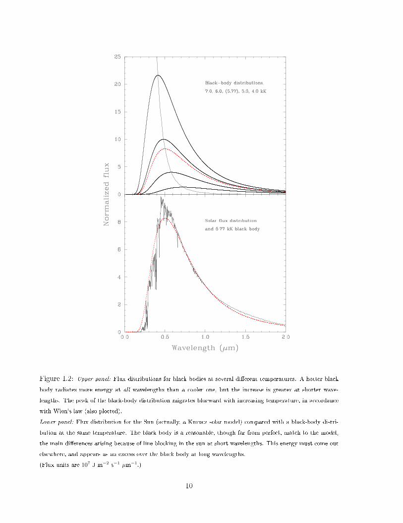
Figure 1.2: Upper panel: Flux distributions for black bodies at several dierent temperatures. A hotter black

body radiates more energy at all wavelengths than a cooler one, but the increase is greater at shorter wave-

lengths. The peak of the black-body distribution migrates blueward with increasing temperature, in accordance

with Wien's law (also plotted).

Lower panel: Flux distribution for the Sun (actually, a Kurucz solar model) compared with a black-body distri-

bution at the same temperature. The black body is a reasonable, though far from perfect, match to the model,

the main dierences arising because of line blocking in the sun at short wavelengths. This energy must come out

elsewhere, and appears as an excess over the black body at long wavelengths.

(Flux units are 107 J m−2 s−1 µm−1.)

10

The Wien approximation to the Planck function is very good at wavelengths shortwards of and up

to the peak of the ux distribution; but one generally needs to go something like ∼ 10× the peak

wavelength before the long-wavelength Rayleigh-Jeans approximation is satisfactory.

1.6.3 Wien's Law

Wien's displacement law (not to be confused with the Wien approximation!) relates the

black-body temperature to the wavelength of peak emission. To nd the peak, we dierentiate

eqtn. (1.17) with respect to wavelength, and set to zero:

∂B

∂λ= 8hc

„hc

λ7kT

exp hc/λkT(exp hc/λkT − 1)2

− 1

λ6

5

exp hc/λkT − 1

«= 0

whence

hc

λmaxkT(1− exp −hc/λmaxkT)−1 − 5 = 0

An analytical solution of this equation can be obtained in terms of the Lambert W function; we

merely quote the result,

λmax

µm=

2898

T/K

We expect the Sun's output to peak around 500 nm (for Teff = 5770 K) just where the human

eye has peak sensitivity, for obvious evolutionary reasons.

1.7 Radiation Energy Density, Uν

Consider some volume of space containing a given number of photons; the photons have energy,

so we can discuss the density of radiant energy. From eqtn. (1.1), and referring to Fig. 1.1,

dEν = Iν(θ) dS dt dν dΩ.

We can eliminate the time dependence2 by noting that there is a single-valued correspondence3

between time and distance for radiation. Dening a characteristic length ` = ct, dt = d`/c, and

dEν = Iν(θ) dSd`cdν dΩ

=Iν(θ)

cdV dν dΩ (1.24)

where the volume element dV = dS d`. The mean radiation energy density per unit frequency

per unit volume is then

Uν dν =1V

∫V

∫ΩdEν

=1c

∫Ω

Iν dν dΩ

2Assuming that no time dependence exists; that is, that for every photon leaving some volume of space, a

compensating photon enters. This is an excellent approximation under many circumstances.3Well, nearly single-valued; the speed at which radiation propagates actually depends on the refractive index

of the medium through which it moves e.g., the speed of light in water is only 3c/4.

11

whence

Uν =1c

∫Iν dΩ

=4π

cJν [J m−3 Hz−1] [from eqtn. (1.2): Jν = 1/4π

∫Iν dΩ] (1.25)

Again, this is explicitly frequency dependent; the total energy density is obtained by integrating

over frequency:

U =

∞∫0

Uν dν.

For black-body radiation, Jν(= Iν) = Bν , and

U =

∞∫0

4π

cBν dν

but∫

πBν = σT 4 (eqtn. (1.21)) so

U =4σ

cT 4 ≡ aT 4

= 7.55× 10−16 T 4 J m−3 (1.26)

where T is in kelvin, σ is the Stefan-Boltzmann constant and a is the `radiation constant'. Note

that the energy density of black-body radiation is a xed quantity (for a given temperature).

For a given form of spectrum, the energy density in radiation must correspond to a specic

number density of photons:

Nphoton =

∞∫0

Uν

hνdν.

For the particular case of a black-body spectrum,

Nphoton ' 2× 107 T 3 photons m−3. (1.27)

Dividing eqtn. (1.26) by (1.27) gives the mean energy per photon for black-body radiation,

hν = 3.78× 10−23T = 2.74kT (1.28)

(although there is, of course, a broad spread in energies of individual photons).

12

1.8 Radiation Pressure

A photon carries momentum E/c (= hν/c).4 Momentum ux (momentum per unit time, per

unit area) is a pressure.5 If photons encounter a surface at some angle θ to the normal, the

component of momentum perpendicular to the surface per unit time per unit area is that

pressure,

dPν =dEν

c× cos θ

1dt dA dν

(where we have chosen to express the photon pressure `per unit frequency'); but the specic

intensity is

Iν =dEν

dA cos θ dΩ dν dt, (1.1)

whence

dPν =Iν

ccos2 θ dΩ

i.e.,

Pν =1c

∫Iνµ

2 dΩ [J m−3 Hz−1 ≡Pa Hz−1] (1.29)

We know that∫dΩ =

2π∫0

+1∫−1

dµ dφ (1.4)

so

Pν =2π

c

∫ +1

−1Iνµ

2 dµ;

however, the K integral is

Kν =12

+1∫−1

Iν(µ)µ2 dµ (1.14)

(from Section 1.4), hence

Pν =4π

cKν (1.30)

4Classically, momentum is mass times velocity. From E = mc2 = hν, the photon rest mass is hν/c2, and its

velocity is c, hence momentum is hν/c.5Dimensional arguments show this to be true; in the SI system, momentum has units of kg m s−1, and

momentum ux has units of kg m s−1, m−2, s−1; i.e., kg m−1 s−2,= N m−2 = Pa the units of pressure.

Pressure in turn is force per unit area (where force is measured in Newtons, = J m−1 = kg m s−2).

13

For an isotropic radiation eld Kν = 1/3Iν = 1/3Jν (eqtn. (1.15)), and so

Pν =4π

3cIν =

4π

3cJν .

In this isotropic case we also have

Uν =4π

cJν =

4π

cIν

(eqtn. (1.25)) so for an isotropic radiation eld the radiation pressure is

Pν =13Uν

or, integrating over frequency (using∫

Uν dν = aT 4 = 4σ/cT 4; eqtn. (1.26)),

PR =13aT 4 =

4σ

3cT 4 [J m−3 ≡ N m−2 ≡ Pa]. (1.31)

In that equation (1.31) expresses the relationship between pressure and temperature, it is the

equation of state for radiation.

Note that in the isotropic case, Pν (or PR) is a scalar quantity it has magnitude but not

direction (like air pressure, locally, on Earth). For an anisotropic radiation eld, the radiation

pressure has a direction (normally outwards from a star), and is a vector quantity. (This

directed pressure, or force per unit area, becomes important in luminous stars, where the force

becomes signicant compared to gravity; Section 11.9.)

14

Section 2

The interaction of radiation with

matter

As a beam of radiation traverses astrophysical material (such as a stellar interior, a stellar

atmosphere, or interstellar space), energy can be added or subtracted the process of `radiative

transfer'. A large number of detailed physical processes can contribute to these changes in

intensity, and we will consider some of these processes in subsequent sections. First, though, we

concentrate on general principles.

2.1 Emission: increasing intensity

A common astrophysical1 denition of the (monochromatic) emissivity is the energy generated

per unit volume,2 per unit time, per unit frequency, per unit solid angle:

jν =dEν

dV dt dν dΩ[J m−3 s−1 Hz−1 sr−1]; (2.1)

If an element of distance along a line (e.g., the line of sight) is ds, then the change in specic

intensity along that element resulting from the emissivity of a volume of material of unit

cross-sectional area is

dIν = +jν(s) ds (2.2)

1Other denitions of `emissivity' occur in physics.2The emissivity can also be dened per unit mass (or, in principle, per particle).

15

2.2 Extinction: decreasing intensity

`Extinction' is a general term for the removal of light from a beam. Two dierent classes of

process contribute to the extinction: absorption and scattering. Absorption (sometimes called

`true absorption') results in the destruction of photons; scattering merely involves redirecting

photons in some new direction. For a beam directed towards the observer, scattering still has

the eect of diminishing the recorded signal, so the two types of process can be treated

together for the present purposes.

The amount of intensity removed from a beam by extinction in (say) a gas cloud must depend

on

The initial strength of the beam (the more light there is, the more you can remove)

The number of particles (absorbers)

The microphysics of the particles specically, how likely they are to absorb (or scatter)

an incident photon. This microphysics is characterized by an eective cross-section per

particle presented to the radiation.

By analogy with eqtn. (2.2), we can write the change in intensity along length ds as

dIν = −aνnIν ds (2.3)

for a number density of n extinguishing particles per unit volume, with aν the `extinction

coecient', or cross-section (in units of area) per particle.

2.3 Opacity

In astrophysical applications, it is customary to combine the cross-section per particle (with

dimensions of area) and the number of particles into either the extinction per unit mass, or the

extinction per unit volume. In the former case we can set

aνn ≡ κνρ

and thus write eqtn. (2.3) as

dIν = −κνρ(s)Iν ds

for mass density ρ, where κν is the (monochromatic) mass extinction coecient or, more

usually, the opacity per unit mass (dimensions of area per unit mass; SI units of m2 kg−1).

16

For opacity per unit volume we have

aνn ≡ kν

whence

dIν = −kνIν ds.

The volume opacity kν has dimensions of area per unit volume, or SI units of m−1. It has a

straightforward and useful physical interpretation; the mean free path for a photon moving

through a medium with volume opacity kν is

`ν ≡ 1/kν. (2.4)

[In the literature, κ is often used generically to indicate opacity, regardless of whether `per unit

mass' or `per unit volume', and the sense has to be inferred from the context. (You can always

do this by looking at the dimensions involved.)]

2.3.1 Optical depth

We can often calculate, but rarely measure, opacity as a function of position along a given

path. Observationally, often all that is accessible is the cumulative eect of the opacity

integrated along the line of sight; this is quantied by the optical depth,

τν =∫ D

0kν(s) ds =

∫ D

0κν ρ(s) ds =

∫ D

0aν n(s) ds (2.5)

over distance D.

2.3.2 Opacity sources

At the atomic level, the processes which contribute to opacity are:

• bound-bound absorption (photoexcitation line process);

• bound-free absorption (photoionization continuum process);

• free-free absorption (continuum process); and

• scattering (continuum process).

17

Absorption process can be thought of as the destruction of photons (through conversion into

other forms of energy, whether radiative or kinetic).

Scattering is the process of photon absorption followed by prompt re-emission through the

inverse process. For example, resonance-line scattering is photo-excitation from the ground

state to an excited state, followed quickly by radiative decay. Continuum scattering processes

include electron scattering and Rayleigh scattering.

Under most circumstances, scattering involves re-emission of a photon with virtually the same

energy (in the rest frame of the scatterer), but in a new direction.3

Calculation of opacities is a major task, but at the highest temperatures (T & 107 K) elements

are usually almost fully ionized, so free-free and electron-scattering opacities dominate. Under

these circumstances, κ ' constant. Otherwise, a parameterization of the form

κ = κ0ρaT b (2.6)

is convenient for analytical or illustrative work.

3In Compton scattering, energy is transferred from a high-energy photon to the scattering electron (or vice

versa for inverse Compton scattering). These processes are important at X-ray and γ-ray energies; at lower

energies, classical Thomson scattering dominates. For our purposes, `electron scattering' can be regarded as

synonymous with Thomson scattering.

18

Rate coecients and rate equations (reference/revision

only)

Before proceeding to consider specic astrophysical environments, we review the coecients

relating to bound-bound (line) transitions. Bound-free (ionization) process will be considered in

sections 5 (photoionization) and 10.2 (collisional ionization).

Einstein (radiative) coecients

Einstein (1916) proposed that there are three purely radiative processes which may be involved in

the formation of a spectral line: induced emission, induced absorption, and spontaneous emission,

each characterized by a coecient reecting the probability of a particular process.

[1] Aji (s−1): the Einstein coecient, or transition probability, for spontaneous decay from an

upper state j to a lower state i, with the emission of a photon (radiative decay); the time

taken for an electron in state j to spontaneously decay to state i is 1/Aji on average

If nj is the number density of atoms in state j then the change in the number density of

atoms in that state per unit time due to spontaneous emission will be

dnj

dt= −

Xi<j

Ajinj

while level i is populated according to

dni

dt= +

Xj>i

Ajinj

[2] Bij (s−1 J−1 m2 sr): the Einstein coecient for radiative excitation from a lower state i to

an upper state j, with the absorption of a photon.

dni

dt= −

Xj>i

BijniIν ,

dnj

dt= +

Xi<j

BijniIν

[3] Bji (s−1 J−1 m2 sr): the Einstein coecient for radiatively induced de-excitation from an

upper state to a lower state.

dnj

dt= −

Xi<j

BjinjIν ,

dni

dt= +

Xj>i

BjinjIν

where Iν is the specic intensity at the frequency ν corresponding to Eij , the energy dierence

between excitation states.

For reference, we state, without proof, the relationships between these coecients:

Aji =2hν3

c2Bji;

Bijgi = Bjigj

where gi is the statistical weight of level i.

19

In astronomy, it is common to work not with the Einstein A coecient, but with the absorption

oscillator strength fij , where

Aji =8π2e2ν2

mec3gi

gjfij

and fij is related to the absorption cross-section by

aij ≡Zaν dν =

πe2

mecfij .

Because of the relationships between the Einstein coecients, we also have

Bij =4π2e2

mehνcfij ,

Bji =4π2e2

mehνc

gi

gjfij

Collisional coecients

For collisional processes we have analogous coecients:

[4] Cji (m3 s−1): the coecient for collisional de-excitation from an upper state to a lower state.

dnj

dt= −

Xj>i

Cjinjne,

dni

dt= +

Xi<j

Cjinjne

(for excitation by electron collisions)

[5] Cij (m3 s−1): the coecient for collisional excitation from a lower state to an upper state.

dni

dt= −

Xj>i

Cijnine,

dnj

dt= +

Xi<j

Cijnine

These coecients are related through

Cij

Cji=gj

giexp

− hν

kTex

fffor excitation temperature Tex.

The rate coecient has a Boltzmann-like dependence on the kinetic temperature

Cij(Tk) =

„2π

Tk

«1/2h2

4π2m3/2e

Ω(ij)

giexp

−∆Eij

kTk

ff∝ 1√

Te

exp

−∆Eij

kTk

ff[m3 s−1] (2.7)

where Ω(1, 2) is the so-called `collision strength'.

Statistical Equilibrium

Overall, for any ensemble of atoms in equilibrium, the number of de-excitations from any given

excitation state must equal the number of excitations into that state the principle of statistical

equilibrium. That is,Xj>i

BijniIν +Xj 6=i

Cijnine =Xj>i

Ajinj +Xj>i

BjinjIν +Xj 6=i

Cjinjne (2.8)

20

Section 3

Radiative transfer

3.1 Radiative transfer along a ray

Iν IνIν

Sd

τ(ν)=0 τ(ν)

+

d

S

Consider a beam of radiation from a distant point source (e.g., an unresolved star), passing

through some intervening material (e.g., interstellar gas). The intensity change as the radiation

traverses the element of gas of thickness ds is the intensity added, less the intensity taken away

(per unit frequency, per unit time, per unit solid angle):

dIν (((((((( dA dν dω dt) = + jν ds(((((((

dA dν dω dt

− kν Iν ds(((((((dA dν dω dt

i.e.,

dIν = (jν − kν Iν) ds,

21

or

dIν

ds= jν − kνIν , (3.1)

which is the basic form of the Equation of Radiative Transfer.

The ratio jν/kν is called the Source Function, Sν . For systems in thermodynamic equilibrium

jν and kν are related through the Kirchho relation,

jν = kνBν(T ),

and so in this case (though not in general) the source function is given by the Planck function

Sν = Bν

Equation (3.1) expresses the intensity of radiation as a function of position. In astrophysics, we

often can't establish exactly where the absorbers are; for example, in the case of an absorbing

interstellar gas cloud of given physical properties, the same absorption lines will appear in the

spectrum of some background star, regardless of where the cloud is along the line of sight. It's

therefore convenient to divide both sides of eqtn. 3.1 by kν ; then using our denition of optical

depth, eqtn. (2.5), gives a more useful formulation,

dIν

dτν= Sν − Iν . (3.2)

3.1.1 Solution 1: jν = 0

We can nd simple solutions for the equation of transfer under some circumstances. The very

simplest case is that of absorption only (no emission; jν = 0), which is appropriate for

interstellar absorption lines (or headlights in fog); just by inspection, eqtn. (3.1) has the

straightforward solution

Iν = Iν(0) exp −τν . (3.3)

We see that an optical depth of 1 results in a reduction in intensity of a factor e−1 (i.e., a factor

∼ 0.37).

3.1.2 Solution 2: jν 6= 0

To obtain a more general solution to transfer along a line we begin by guessing that

Iν = F exp C1τν (3.4)

22

where F is some function to be determined, and C1 some constant; dierentiating eqtn. 3.4,

dIν

dτν= exp C1τν

dFdτν

+ FC1 exp C1τν

= exp C1τνdFdτν

+ C1Iν , = Sν − Iν (eqtn. 3.2).

Identifying like terms we see that C1 = −1 and that

Sν = exp −τνdFdτν

,

i.e.,

F =

Z τν

0

Sν exp tνdtν + C2

where t is a dummy variable of integration and C2 is some constant. Referring back to eqtn. (3.4),

we now have

Iν(τν) = exp −τνZ τν

0

Sν(tν) exp tν dtν + Iν(0) exp −τν

where the constant of integration is set by the boundary condition of zero extinction (τν = 0). In

the special case of Sν independent of τν we obtain

Iν = Iν(0) exp −τν+ Sν (1− exp −τν)

3.2 Radiative Transfer in Stellar Atmospheres

Having established the principles of the simple case of radiative transfer along a ray, we turn to

more general circumstances, where we have to consider radiation coming not just from one

direction, but from arbitrary directions. The problem is now three-dimensional in principle; we

could treat it in cartesian (xyz) coördinates,1 but because a major application is in spherical

objects (stars!), it's customary to use spherical polar coördinates.

Again consider a beam of radiation travelling in direction s, at some angle θ to the radial

direction in a stellar atmosphere (Fig. 3.1). If we neglect the curvature of the atmosphere (the

`plane parallel approximation') and any azimuthal dependence of the radiation eld, then the

intensity change along this particular ray is

dIν

ds= jν − kνIν , (3.1)

as before.

We see from the gure that

dr = cos θ ds ≡ µds

1We could also treat the problem as time-dependent; but we won't . . . A further complication that we won't

consider is motion in the absorbing medium (which introduces a directional dependence in kν and jν); this

directionality is important in stellar winds, for example.

23

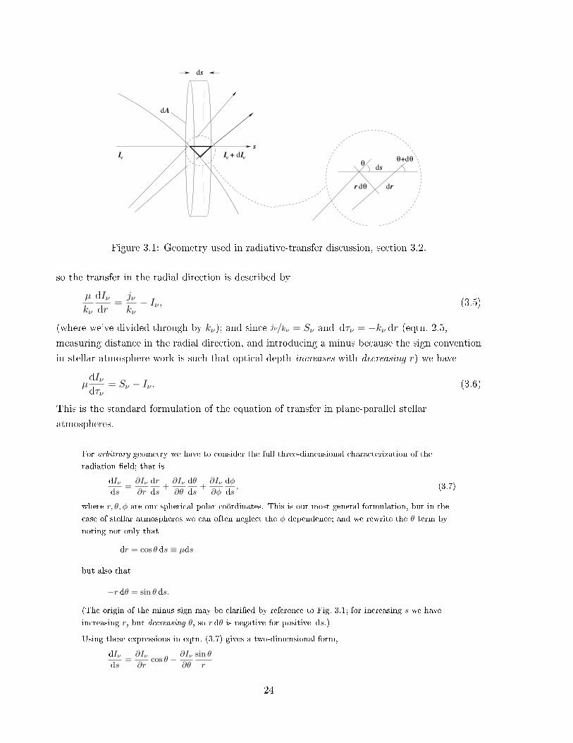
IνIν

+ dIν

ds

ds

drdθr

dθθ+

Ad

s

θ

Figure 3.1: Geometry used in radiative-transfer discussion, section 3.2.

so the transfer in the radial direction is described by

µ

kν

dIν

dr=

jν

kν− Iν , (3.5)

(where we've divided through by kν); and since jν/kν = Sν and dτν = −kν dr (eqtn. 2.5,

measuring distance in the radial direction, and introducing a minus because the sign convention

in stellar-atmosphere work is such that optical depth increases with decreasing r) we have

µdIν

dτν= Sν − Iν . (3.6)

This is the standard formulation of the equation of transfer in plane-parallel stellar

atmospheres.

For arbitrary geometry we have to consider the full three-dimensional characterization of the

radiation eld; that is

dIν

ds=∂Iν

∂r

dr

ds+∂Iν

∂θ

dθ

ds+∂Iν

∂φ

dφ

ds, (3.7)

where r, θ, φ are our spherical polar coördinates. This is our most general formulation, but in the

case of stellar atmospheres we can often neglect the φ dependence; and we rewrite the θ term by

noting not only that

dr = cos θ ds ≡ µds

but also that

−r dθ = sin θ ds.

(The origin of the minus sign may be claried by reference to Fig. 3.1; for increasing s we have

increasing r, but decreasing θ, so r dθ is negative for positive ds.)

Using these expressions in eqtn. (3.7) gives a two-dimensional form,

dIν

ds=∂Iν

∂rcos θ − ∂Iν

∂θ

sin θ

r

24

but this is also

= jν − kνIν

so, dividing through by kν as usual,

cos θ

kν

∂Iν

∂r+

sin θ

kνr

∂Iν

∂θ=jνkν− Iν

= Sν − Iν

Once again, it's now useful to think in terms of the optical depth measured radially inwards:

dτ = −kν dr,

which gives us the customary form of the equation of radiative transfer for use in extended stellar

atmospheres, for which the plane-parallel approximation fails:

sin θ

τν

∂Iν

∂θ− µ

∂Iν

∂τν= Sν − Iν . (3.8)

We recover our previous, plane-parallel, result if the atmosphere is very thin compared to the

stellar radius. In this case, the surface curvature shown in Fig. 3.1 becomes negligible, and dθ

tends to zero. Equation (3.8) then simplies to

µ∂Iν

∂τν= Iν − Sν , (3.6)

which is our previous formulation of the equation of radiative transfer in plane-parallel stellar

atmospheres.

3.3 Energy transport in stellar interiors

3.3.1 Radiative transfer

In optically thick environments in particular, stellar interiors radiation is often the

most important transport mechanism,2 but for large opacities the radiant energy

doesn't ow directly outwards; instead, it diuses slowly outwards.

The same general principles apply as led to eqtn. (3.6); there is no azimuthal

dependence of the radiation eld, and the photon mean free path is (very) short

compared to the radius. Moreover, we can make some further simplications. First,

the radiation eld can be treated as isotropic to a very good approximation. Secondly,

the conditions appropriate to `local thermodynamic equilibrium' (LTE; Sec. 10.1)

apply, and the radiation eld is very well approximated by black-body radiation.

2Convection can also be a signicant means of energy transport under appropriate conditions, and is discussed

in Section 3.3.3.

25

Box 3.1. It may not be immediately obvious that the radiation eld in stellar interiors is, essentially,

isotropic; after all, outside the energy-generating core, the full stellar luminosity is transmitted across

any spherical surface of radius r. However, if this ux is small compared to the local mean intensity,

then isotropy is justied.

The ux at an interior radius r (outside the energy-generating core) must equal the ux at R (the

surface); that is,

πF = σT 4effR2

r2

while the mean intensity is

Jν(r) ' Bν(T (r)) = σT 4(r).

Their ratio is

F

J=

„Teff

T (r)

«4 „R

r

«2

.

Temperature rises rapidly below the surface of stars, so this ratio is always small; for example, in

the Sun, T (r) ' 3.85 MK at r = 0.9R, whence F/J ' 10−11. That is, the radiation eld is isotropic

to better than 1 part in 1011.

We recall that, in general, Iν is direction-dependent; i.e., is Iν(θ, φ) (although we have

generally dropped the explicit dependence for economy of nomenclature). Multiplying

eqtn. (3.6) by cos θ and integrating over solid angle, using dΩ = sin θ dθ dφ = dµ dφ,

then

d

dτν

Z 2π

0

Z +1

−1

µ2Iν(µ, φ)dµ dφ =

Z 2π

0

Z +1

−1

µIν(µ, φ)dµ dφ−Z 2π

0

Z +1

−1

µSν(µ, φ)dµ dφ;

or, for axial symmetry,

d

dτν

Z +1

−1

µ2Iν(µ)dµ =

Z +1

−1

µIν(µ)dµ−Z +1

−1

µSν(µ)dµ.

Using eqtns. (1.14) and (1.9), respectively, for the rst two terms, and supposing that

the emissivity has no preferred direction (as is true to an excellent aproximation in

stellar interiors; Box 3.1) so that the source function is isotropic (and so the nal term

is zero), we obtain

dKν

dτν=Fν

4π

or, from eqtn. (1.15),

1

3

dIν

dτν=Fν

4π.

In LTE we may set Iν = Bν(T ), the Planck function; and dτν = −kν dr (where again

the minus arises because the optical depth is measured inwards, and decreases with

increasing r). Making these substitutions, and integrating over frequency,Z ∞

0

Fν dν = −4π

3

Z ∞

0

1

kν

dBν(T )

dT

dT

drdν (3.9)

To simplify this further, we introduce the Rosseland mean opacity, kR, dened by

1

kR

Z ∞

0

dBν(T )

dTdν =

Z ∞

0

1

kν

dBν(T )

dTdν.

26

Recalling thatZ ∞

0

πBν dν = σT 4 (1.21)

we also haveZ ∞

0

dBν(T )

dTdν =

d

dT

Z ∞

0

Bν(T )dν

=4σT 3

π

so that eqtn. 3.9 can be written asZ ∞

0

Fν dν = −4π

3

1

kR

dT

dr

acT 3

π(3.10)

where a is the radiation constant, 4σ/c.

The luminosity at some radius r is given by

L(r) = 4πr2Z ∞

0

Fν dν

so, nally,

L(r) = −16π

3

r2

kR

dT

dracT 3, (3.11)

which is our adopted form of the equation of radiative energy transport.

Box 3.2. The radiative energy density is U = aT 4 (eqtn. 1.26), so that dU/dT = 4aT 3, and we can

express eqtn. (3.10) as

F =

Z ∞

0

Fν dν

= − c

3kR

dT

dr

dU

dT

= − c

3kR

dU

dr

This `diusion approximation' shows explicitly how the radiative ux relates to the energy gradient;

the constant of proportionality, c/3kR, is called the diusion coecient. The larger the opacity, the

less the ux of radiative energy, as one might intuitively expect.

3.3.2 Convection in stellar interiors

Energy transport can take place through one of three standard physical processes:

radiation, convection, or conduction. In the raried conditions of interstellar space,

radiation is the only signicant mechanism; and gases are poor conductors, so

conduction is generally negligible even in stellar interiors (though not in, e.g.,

neutron stars). In stellar interiors (and some stellar atmospheres) energy transport

by convection can be very important.

27

Conditions for convection to occur

We can rearrange eqtn. (3.11) to nd the temperature gradient where energy

transport is radiative:

dTdr

= − 316π

kR

r2

L(r)acT 3

,

If the energy ux isn't contained by the temperature gradient, we have to invoke

another mechanism convection for energy transport. (Conduction is negligible

in ordinary stars.) Under what circumstances will this arise?

Suppose that through some minor perturbation, an element (or cell, or blob, or

bubble) of gas is displaced upwards within a star. It moves into surroundings at

lower pressure, and if there is no energy exchange it will expand and cool

adiabatically. This expansion will bring the system into pressure equilibrium (a

process whose timescale is naturally set by the speed of sound and the linear scale

of the perturbation), but not necessarily temperature equilibrium the cell (which

arose in deeper, hotter layers) may be hotter and less dense than its surroundings.

If it is less dense, then simple buoyancy comes into play; the cell will continue to

rise, and convective motion occurs.3

We can establish a condition for convection by conmsidering a discrete bubble of

gas moving upwards within a star, from radius r to r + dr. We suppose that the

pressure and density of the ambient background and within the bubble are

(P1, ρ1), (P2, ρ2) and (P ∗1 , ρ∗1), (P ∗

2 , ρ∗2),respectively, at (r), (r + dr).

The condition for adiabatic expansion is that

PV γ = constant

where γ = CP /CV , the ratio of specic heats at constant pressure and constant

volume. (For a monatomic ideal gas, representative of stellar interiors, γ = 5/3.)

Thus, for a blob of constant mass (V ∝ ρ−1),

P ∗1

(ρ∗1)γ =

P ∗2

(ρ∗2)γ ; i.e.,

(ρ∗2)γ =

P ∗2

P ∗1

(ρ∗1)γ .

A displaced cell will continue to rise if ρ∗2 < ρ2. However, from our discussion above,

we suppose that P ∗1 = P1, ρ∗1 = ρ1 initially; and that P ∗

2 = P2 nally. Thus

3Another way of looking at this is that the entropy (per unit mass) of the blob is conserved, so the star is

unstable if the ambient entropy per unit mass decreases outwards.

28

convection will occur if

(ρ∗2)γ =

P2

P1(ρ1)γ < ρ2.

Setting P2 = P1 − dP , ρ2 = ρ1 − dρ, we obtain the condition

ρ1

(1− dP

P1

)1/γ

< ρ1 − dρ.

If dP P1, then a binomial expansion gives us(1− dP

P

)1/γ

' 1− 1γ

dPP

(where we have dropped the now superuous subscript), and so

−ρ

γ

dPP

< −dρ, or

−1γ

1P

dPdr

< −1ρ

dρdr

(3.12)

However, the equation of state of the gas is P ∝ ρT , i.e.,

dPP

=dρρ

+dTT

, or

1P

dPdr

=1ρ

dρdr

+1T

dTdr

;

thus, from eqtn. (3.12),

1P

dPdr

<1γ

1P

dPdr

+1T

dTdr

<

(γ

γ − 1

)1T

dTdr

, or (3.13)

d(lnP ))d(lnT )

<γ

γ − 1

for convection to occur.

Schwarzschild criterion

Start with adiabatic EOS

Pρ−γ = constant (3.14)

i.e.,

d ln ρ

d lnP=

1γ

(3.15)

29

To rise, the cell density must decrease more rapidly than the ambient density; i.e.,

d ln ρc

d lnPc>

d ln ρa

d lnPa(3.16)

Gas law, P = nkT = ρkT/µ gives

d ln ρ

d lnP= 1 +

d lnµ

d lnP− d lnT

d lnP(3.17)

whence the Schwarzschild criterion for convection,

d lnTa

d lnPa> 1− 1

γ+

d lnµ

d lnP. (3.18)

3.3.3 Convective energy transport

Convection is a complex, hydrodynamic process. Although much progress is being

made in numerical modelling of convection over short timescales, it's not feasible at

present to model convection in detail in stellar-evolution codes, because of the vast

disparities between convective and evolutionary timescales. Instead, we appeal to

simple parameterizations of convection, of which mixing-length `theory' is the most

venerable, and the most widely applied.

We again consider an upwardly moving bubble of gas. As it rises, a temperature

dierence is established with the surrounding (cooler) gas, and in practice some

energy loss to the surroundings must occur.

XXXWork in progress

30