Particle Motion in Colloidal Dispersions: Applications toMicrorheology and Nonequilibrium Depletion Interactions.

Thesis by

Aditya S. Khair

In Partial Fulfillment of the Requirements

for the Degree of

Doctor of Philosophy

California Institute of Technology

Pasadena, California

2007

(Defended February 6, 2007)

ii

c© 2007

Aditya S. Khair

All Rights Reserved

iii

Acknowledgements

The past four and one-third years I have spent at Caltech have been among the most enjoy-

able of my life. Many people have contributed to this; unfortunately, I cannot acknowledge

each and every person here. I offer my most sincere apologies to those whom I (through

ignorance) do not mention below.

Firstly, I wish to thank my thesis adviser, John Brady. John gave me a fantastic

research project to work on; allowed me generous vacation time to go back to England; and

was always available to talk. As a researcher, John’s integrity, curiosity, and rigor serve as

the standard that I shall aspire to throughout my professional life.

I would also like to thank the members of my thesis committee — John Seinfeld, Todd

Squires, and Zhen-Gang Wang — for their support and interest in my work. In particular,

Todd was instrumental in sparking my interest in microrheology and has given me much

advice on pursuing a career in academia.

I have been fortunate enough to share the highs and lows of graduate school with some

great friends. I thank the members of the Brady research group that I have overlapped

with: Josh Black, Ileana Carpen, Alex Leshansky, Ubaldo Cordova, James Swan, Manuj

Swaroop, and Andy Downard, for making the sub-basement of Spalding an enjoyable place

to work. I also thank Alex Brown, Justin Bois, Rafael Verduzco, Mike Feldman, and Akira

Villar for sharing many laughs (and many beers) over the years.

iv

All of the Chemical Engineering staff receive my most sincere thanks. In particular, the

graduate-student secretary, Kathy Bubash, and our computer expert, Suresh Guptha, have

helped me greatly.

A special thanks goes to Hilda and Sal Martinez, the parents of my fiancee, Vanessa

(see below). Hilda and Sal have treated me so kindly and always welcomed me into their

home. I will be forever grateful.

I would not have reached this point without the love of my parents. From an early age,

they emphasized to me the importance of a good education; furthermore, they provided me

every opportunity to get one. Their continued support and encouragement means more to

me than they will ever know.

The last, but certainly not the least, acknowledgment goes to the love of my life, Vanessa.

She is the one person who can always put on a smile on my face when I am feeling low. I

hope that many years from now we can both look back on my time at Caltech with fond

memories.

v

Abstract

Over the past decade, microrheology has burst onto the scene as a technique to interro-

gate and manipulate complex fluids and biological materials at the micro- and nano-meter

scale. At the heart of microrheology is the use of colloidal ‘probe’ particles embedded in

the material of interest; by tracking the motion of a probe one can ascertain rheological

properties of the material. In this study, we propose and investigate a paradigmatic model

for microrheology: an externally driven probe traveling through an otherwise quiescent col-

loidal dispersion. From the probe’s motion one can infer a ‘microviscosity’ of the dispersion

via application of Stokes drag law. Depending on the amplitude and time-dependence of

the probe’s movement, the linear or nonlinear (micro-)rheological response of the dispersion

may be inferred: from steady, arbitrary-amplitude motion we compute a nonlinear micro-

viscosity, while small-amplitude oscillatory motion yields a frequency-dependent (complex)

microviscosity. These two microviscosities are shown, after appropriate scaling, to be in

good agreement with their (macro)-rheological counterparts. Furthermore, we investigate

the role played by the probe’s shape — sphere, rod, or disc — in microrheological experi-

ments.

Lastly, on a related theme, we consider two spherical probes translating in-line with

equal velocities through a colloidal dispersion, as a model for depletion interactions out of

equilibrium. The probes disturb the tranquility of the dispersion; in retaliation, the disper-

vi

sion exerts a entropic (depletion) force on each probe, which depends on the velocity of the

probes and their separation. When moving ‘slowly’ we recover the well-known equilibrium

depletion attraction between probes. For ‘rapid’ motion, there is a large accumulation of

particles in a thin boundary layer on the upstream side of the leading probe, whereas the

trailing probe moves in a tunnel, or wake, of particle-free solvent created by the leading

probe. Consequently, the entropic force on the trailing probe vanishes, while the force on

the leading probe approaches a limiting value, equal to that for a single translating probe.

vii

Contents

Acknowledgements iii

Abstract v

1 Introduction 1

1.1 Introduction . . . . . . . . . . . . . . . . . . . . . . . . . . . . . . . . . . . . 2

1.2 Bibliography . . . . . . . . . . . . . . . . . . . . . . . . . . . . . . . . . . . 10

2 Single particle motion in colloidal dispersions: a simple model for active

and nonlinear microrheology 13

2.1 Introduction . . . . . . . . . . . . . . . . . . . . . . . . . . . . . . . . . . . . 14

2.2 Nonequilibrium microstructure . . . . . . . . . . . . . . . . . . . . . . . . . 21

2.3 Average velocity of the probe particle and its interpretation as a microviscosity 26

2.4 Nonequilibrium microstructure and microrheology at small Peb . . . . . . . 32

2.4.1 Perturbation expansion of the structural deformation . . . . . . . . . 32

2.4.2 Linear response: The intrinsic microviscosity and its relation to self-

diffusivity . . . . . . . . . . . . . . . . . . . . . . . . . . . . . . . . . 38

2.4.3 Weakly nonlinear theory . . . . . . . . . . . . . . . . . . . . . . . . . 44

2.5 Numerical solution of the Smoluchowski equation for arbitrary Peb . . . . . 46

2.5.1 Legendre polynomial expansion . . . . . . . . . . . . . . . . . . . . . 48

viii

2.5.2 Finite difference methods . . . . . . . . . . . . . . . . . . . . . . . . 51

2.6 Results . . . . . . . . . . . . . . . . . . . . . . . . . . . . . . . . . . . . . . . 53

2.6.1 No hydrodynamic interactions . . . . . . . . . . . . . . . . . . . . . 53

2.6.2 The effect of hydrodynamic interactions . . . . . . . . . . . . . . . . 57

2.7 Discussion . . . . . . . . . . . . . . . . . . . . . . . . . . . . . . . . . . . . . 68

2.8 Bibliography . . . . . . . . . . . . . . . . . . . . . . . . . . . . . . . . . . . 75

Appendices to chapter 2 78

2.A The Brownian velocity contribution . . . . . . . . . . . . . . . . . . . . . . . 79

2.B Finite difference method . . . . . . . . . . . . . . . . . . . . . . . . . . . . . 80

2.C Boundary-layer equation . . . . . . . . . . . . . . . . . . . . . . . . . . . . . 83

2.D Boundary-layer analysis of the pair-distribution function at high Peb in the

absence of hydrodynamic interactions . . . . . . . . . . . . . . . . . . . . . 85

2.E Boundary-layer analysis of the pair-distribution function at high Peb for b ≡ 1 88

3 “Microviscoelasticity” of colloidal dispersions 93

3.1 Introduction . . . . . . . . . . . . . . . . . . . . . . . . . . . . . . . . . . . . 94

3.2 Governing equations . . . . . . . . . . . . . . . . . . . . . . . . . . . . . . . 101

3.2.1 Smoluchowski equation . . . . . . . . . . . . . . . . . . . . . . . . . 101

3.2.2 Average probe velocity . . . . . . . . . . . . . . . . . . . . . . . . . . 105

3.3 Small-amplitude oscillations . . . . . . . . . . . . . . . . . . . . . . . . . . . 105

3.4 Connection between microviscosity and self-diffusivity of the probe particle 110

3.5 Microstructure & microrheology: No hydrodynamic interactions . . . . . . . 112

3.6 Microstructure & microrheology: Hydrodynamic interactions . . . . . . . . 120

3.7 Scale-up of results to more concentrated dispersions . . . . . . . . . . . . . 129

ix

3.8 Comparison with experimental data . . . . . . . . . . . . . . . . . . . . . . 132

3.9 Discussion . . . . . . . . . . . . . . . . . . . . . . . . . . . . . . . . . . . . . 139

3.10 Bibliography . . . . . . . . . . . . . . . . . . . . . . . . . . . . . . . . . . . 144

Appendix to chapter 3 148

3.A High-frequency asymptotics with hydrodynamic interactions . . . . . . . . . 149

4 Microrheology of colloidal dispersions: shape matters 153

4.1 Introduction . . . . . . . . . . . . . . . . . . . . . . . . . . . . . . . . . . . . 154

4.2 Nonequilibrium microstructure . . . . . . . . . . . . . . . . . . . . . . . . . 158

4.2.1 Prolate probe . . . . . . . . . . . . . . . . . . . . . . . . . . . . . . . 160

4.2.2 Oblate probe . . . . . . . . . . . . . . . . . . . . . . . . . . . . . . . 162

4.3 Microviscosity . . . . . . . . . . . . . . . . . . . . . . . . . . . . . . . . . . . 163

4.4 Analytical results . . . . . . . . . . . . . . . . . . . . . . . . . . . . . . . . . 166

4.4.1 Near equilibrium Pe 1 . . . . . . . . . . . . . . . . . . . . . . . . 166

4.4.2 Far from equilibrium Pe 1 . . . . . . . . . . . . . . . . . . . . . . 168

4.4.2.1 Oblate probe . . . . . . . . . . . . . . . . . . . . . . . . . . 168

4.4.2.2 Prolate probe . . . . . . . . . . . . . . . . . . . . . . . . . . 171

4.5 Numerical methods . . . . . . . . . . . . . . . . . . . . . . . . . . . . . . . . 176

4.5.1 Legendre polynomial expansion . . . . . . . . . . . . . . . . . . . . . 177

4.5.2 Finite differences . . . . . . . . . . . . . . . . . . . . . . . . . . . . . 178

4.6 Results . . . . . . . . . . . . . . . . . . . . . . . . . . . . . . . . . . . . . . . 179

4.7 Discussion . . . . . . . . . . . . . . . . . . . . . . . . . . . . . . . . . . . . . 186

4.8 Bibliography . . . . . . . . . . . . . . . . . . . . . . . . . . . . . . . . . . . 193

x

Appendices to chapter 4 196

4.A Exact solution of the Smoluchowski equation . . . . . . . . . . . . . . . . . 197

4.B Asymptotic analysis at large Pe . . . . . . . . . . . . . . . . . . . . . . . . . 199

4.C Prolate probe translating at an angle to its symmetry axis . . . . . . . . . . 203

5 On the motion of two particles translating with equal velocities through

a colloidal dispersion 209

5.1 Introduction . . . . . . . . . . . . . . . . . . . . . . . . . . . . . . . . . . . . 210

5.2 Governing equations . . . . . . . . . . . . . . . . . . . . . . . . . . . . . . . 213

5.2.1 Nonequilibrium microstructure . . . . . . . . . . . . . . . . . . . . . 213

5.2.2 Forces on the probes . . . . . . . . . . . . . . . . . . . . . . . . . . . 217

5.3 Solution of the Smoluchowski equation . . . . . . . . . . . . . . . . . . . . . 219

5.3.1 Non-intersecting excluded volumes: bispherical coordinates . . . . . 220

5.3.2 Intersecting excluded volumes: toroidal coordinates . . . . . . . . . . 223

5.4 Results . . . . . . . . . . . . . . . . . . . . . . . . . . . . . . . . . . . . . . . 226

5.5 Discussion . . . . . . . . . . . . . . . . . . . . . . . . . . . . . . . . . . . . . 231

5.6 Bibliography . . . . . . . . . . . . . . . . . . . . . . . . . . . . . . . . . . . 237

6 Conclusions 239

6.1 Conclusions & future directions . . . . . . . . . . . . . . . . . . . . . . . . . 240

6.2 Bibliography . . . . . . . . . . . . . . . . . . . . . . . . . . . . . . . . . . . 247

xi

List of Figures

2.1 Sketch of the probe and background/bath particle configuration. . . . . . . . 24

2.2 The O(Peb) structural deformation function f1 for several values of b = b/a. 35

2.3 First O(Pe2b) structural deformation function f2 for several values of b = b/a. 36

2.4 Second O(Pe2b) structural deformation function h2 for several values of b = b/a. 37

2.5 The equilibrium microstructure contribution to the intrinsic hydrodynamic

microviscosity ηHi,0 as a function of the excluded radius b = b/a. . . . . . . . . 41

2.6 Intrinsic microviscosity contributions in the limit Peb → 0 as a function of

b = b/a. . . . . . . . . . . . . . . . . . . . . . . . . . . . . . . . . . . . . . . . 43

2.7 The O(Pe2b) contribution to the intrinsic hydrodynamic microviscosity ηH

i

(2.28) as a function of b = b/a. . . . . . . . . . . . . . . . . . . . . . . . . . . 45

2.8 Structural deformation f(s) = g(s) − 1 in the symmetry plane of the probe

particle as a function of Peb for b = 1.00001. . . . . . . . . . . . . . . . . . . 47

2.9 Angular dependence of the structural deformation at contact for several Peb

in the absence of hydrodynamic interactions. . . . . . . . . . . . . . . . . . . 54

2.10 The pair-distribution function at contact as a function of the polar angle θ

and Peb in the absence of hydrodynamic interactions, b→∞. . . . . . . . . . 56

2.11 The intrinsic microviscosity ηi as a function of Peb in the absence of hydrody-

namic interactions. . . . . . . . . . . . . . . . . . . . . . . . . . . . . . . . . . 57

xii

2.12 Small Peb variation of the intrinsic microviscosity for b = 1.00001. . . . . . . 58

2.13 The pair-distribution function at contact as a function of the polar angle θ

and Peb in the case of near-full hydrodynamic interactions b = 1.00001. . . . 59

2.14 Determination of the scaling exponent δ relating the pair-distribution function

at contact to Peb for various b. . . . . . . . . . . . . . . . . . . . . . . . . . . 61

2.15 Contributions to the intrinsic microviscosity ηi as a function of Peb for various b. 63

2.16 The Brownian intrinsic microviscosity ηBi as a function of Peb and b. . . . . . 66

2.17 The intrinsic microviscosity for b = 1.00001 as a function of Peb. . . . . . . . 68

2.18 Comparison of the microviscosity and macroviscosity. . . . . . . . . . . . . . 70

3.1 O(φb) coefficient of the low-frequency microviscosity η′0 versus b = b/a. . . . . 109

3.2 Real part of the reduced complex viscosity in the absence of hydrodynamic

interactions as a function of dimensionless frequency α. . . . . . . . . . . . . 116

3.3 Imaginary part of the reduced complex viscosity in the absence of hydrody-

namic interactions as a function of dimensionless frequency α. . . . . . . . . 118

3.4 Cox-Merz relationship between the frequency ω and external force F ext de-

pendence of the relative microviscosity increment, ∆ηr = ηr − 1. . . . . . . . 119

3.5 Real part of the reduced complex viscosity versus dimensionless frequency α

for various b = b/a. . . . . . . . . . . . . . . . . . . . . . . . . . . . . . . . . . 121

3.6 Imaginary part of the reduced complex viscosity versus dimensionless fre-

quency α for various b = b/a. . . . . . . . . . . . . . . . . . . . . . . . . . . . 122

3.7 Elastic modulus G′(α)/φb = αη′′(α)/φb versus dimensionless frequency α for

various b = b/a. . . . . . . . . . . . . . . . . . . . . . . . . . . . . . . . . . . 123

3.8 Cox-Merz relationship between the frequency ω and external force F ext de-

pendence of the relative microviscosity increment, ∆T ηr = ηr − (1 + ηH). . . 129

xiii

3.9 Comparison of theoretical calculations and experimental data for the real part

of the reduced complex viscosity, (η′(α∗)−η′∞)/(η′0−η′∞), versus dimensionless

frequency α∗(φb) = ωb2/2Ds∞(φb). . . . . . . . . . . . . . . . . . . . . . . . . 135

3.10 Comparison of theoretical calculations and experimental data for the imagi-

nary part of the reduced complex viscosity, η′′(α∗)/(η′0 − η′∞), versus dimen-

sionless frequency α∗(φb) = ωb2/2Ds∞(φb). . . . . . . . . . . . . . . . . . . . . 137

3.11 Real part of the reduced complex viscosity versus dimensionless ‘rescaled’ fre-

quency α∗ = ωτ . . . . . . . . . . . . . . . . . . . . . . . . . . . . . . . . . . . 138

4.1 Definition sketch for the prolate probe. . . . . . . . . . . . . . . . . . . . . . 161

4.2 Definition sketch for the oblate probe. . . . . . . . . . . . . . . . . . . . . . . 162

4.3 Plot of the mobility factors Kob and Kpr versus probe aspect ratio a = a/b. . 164

4.4 Microviscosity increments at small Pe as a function of probe’s aspect ratio

a = a/b. . . . . . . . . . . . . . . . . . . . . . . . . . . . . . . . . . . . . . . . 167

4.5 Sketch of the microstructure around a oblate probe at large Pe. . . . . . . . 170

4.6 Sketch of the microstructure around an prolate probe at large Pe. . . . . . . 172

4.7 Microviscosity increments at large Pe as a function of probe’s aspect ratio

a = a/b. . . . . . . . . . . . . . . . . . . . . . . . . . . . . . . . . . . . . . . . 174

4.8 Difference in microviscosity increments at small Pe and large Pe as a function

of probe aspect ratio a = a/b. . . . . . . . . . . . . . . . . . . . . . . . . . . . 175

4.9 Sample finite difference gird for a prolate probe. . . . . . . . . . . . . . . . . 178

4.10 Microstructural deformation, g−1, in the symmetry plane of the prolate probe

as a function of Pe. . . . . . . . . . . . . . . . . . . . . . . . . . . . . . . . . 180

4.11 Microstructural deformation, g−1, in the symmetry plane of the oblate probe

as a function of Pe. . . . . . . . . . . . . . . . . . . . . . . . . . . . . . . . . 181

xiv

4.12 Microviscosity increment for a prolate probe, ∆ηprr , as a function of Pe =

Ub/D for different a = a/b. . . . . . . . . . . . . . . . . . . . . . . . . . . . . 182

4.13 Microviscosity increment for an oblate probe, ∆ηobr , as a function of Pe =

Ub/D for different a = a/b. . . . . . . . . . . . . . . . . . . . . . . . . . . . . 183

4.14 Comparison of microviscosity increments from prolate and oblate probes with

the macroviscosity. . . . . . . . . . . . . . . . . . . . . . . . . . . . . . . . . . 187

4.15 Sketch of a prolate probe translating at angle β to its symmetry axis. . . . . 189

5.1 Definition sketch for non-intersecting excluded-volumes, d > 4. . . . . . . . . 221

5.2 Sample finite difference grid in (transformed) bispherical coordinates. . . . . 222

5.3 Definition sketch for intersecting excluded-volumes, d < 4. . . . . . . . . . . . 224

5.4 Sample finite difference grid in (transformed) toroidal coordinates. . . . . . . 225

5.5 Microstructural deformation, g − 1, in the symmetry plane of the probes as a

function of Pe for d = 5. . . . . . . . . . . . . . . . . . . . . . . . . . . . . . . 226

5.6 Microstructural deformation, g − 1, in the symmetry plane of the probes as a

function of Pe for d = 3. . . . . . . . . . . . . . . . . . . . . . . . . . . . . . . 228

5.7 Difference in entropic forces, −(〈∆F zl 〉2 − 〈∆F z

t 〉2)/(φkT/a), versus Pe =

Ua/D3 for various d. . . . . . . . . . . . . . . . . . . . . . . . . . . . . . . . . 229

5.8 Entropic forces, 〈∆F zi 〉2/(φkT/a), versus d for Pe = 0.0001. . . . . . . . . . . 230

5.9 Entropic forces, 〈∆F zi 〉2/(φkT/a), versus Pe for d = 3.5. . . . . . . . . . . . . 231

5.10 Entropic forces, 〈∆F zi 〉2/(φkT/a), versus d for Pe = 5. . . . . . . . . . . . . . 232

xv

List of Tables

2.1 Total ηi; equilibrium ηHi,0; compressional (F ext

r > 0) ηi,c; and extensional

(F extr < 0) ηi,e contributions to the intrinsic microviscosity at Peb = 1000

for full hydrodynamics (b = 1.00001 ≈ 1) and without hydrodynamics (b→∞). 65

3.1 Brief description of the experimental investigations discussed in § 3.8. . . . . 134

1

Chapter 1

Introduction

2

1.1 Introduction

Life isn’t simple: for instance, most fluids do not conform to Newton’s ideal. Such ‘com-

plex fluids’, comprising (sub-) micrometer sized particles suspended in a liquid or gas, are

ubiquitous: blood, inks, slurries, photonic crystals, aerosols, and bio-materials to name

but a few examples. The intricate microstructure — the spatio-temporal configuration of

the suspended particles — possessed by such materials can lead to fascinating and unex-

pected macroscopic (collective) phenomena. Moreover, a thorough knowledge of the mi-

crostructural response of complex fluids to external body forces and ambient flow fields is

of paramount importance, in terms of performance and safety, to the design of industrial,

microfluidic, and bio-medical devices.

The study of the flow and mechanical properties of complex fluids is the field of rheol-

ogy. Over the past decade, a number of experimental techniques have burst onto the scene

with the ability to infer rheological properties of complex fluids at the micro- (and nano-)

meter scale. Collectively, they have come to be known as ‘microrheology’ (MacKintosh and

Schmidt 1999; Waigh 2005). This name was adopted, perhaps, to distinguish these tech-

niques from more traditional (macro-) rheological procedures (e.g. mechanical rheometry),

which operate typically on much larger (millimeter or more) length scales. Therein lies the

main advantage of micro- over macro-rheology: it requires much smaller amounts of sample.

This is a particular advantage for rare, expensive, or biological substances that one simply

cannot produce or procure in quantities sufficient for macrorheological testing.

At the heart of microrheology is the use of colloidal ‘probe’ particles embedded in the

material of interest. Through tracking the motion of the probe (via confocal microscopy,

e.g.) it is possible to infer rheological properties of the material. In passive tracking

3

experiments the probe moves diffusively due to the random thermal fluctuations of its

environment. The mean-squared displacement of the probe is measured, from which the

frequency-dependent shear modulus of the material is inferred via a generalized Stokes-

Einstein-Sutherland relation (Mason and Weitz 1995). Many diverse systems, such as DNA

solutions (Mason et al. 1997), living cells (Caspi et al. 2000; Daniels et al. 2006), and actin

networks (Gittes et al. 1997), have been studied using passive microrheology. One should

not think, however, that the use of thermally diffusing probes is limited to ascertaining

viscoelastic moduli: recent studies have employed them to study protein folding (Tu and

Breedveld 2005), ‘nanohydrodynamics’ at interfaces (Joly et al. 2006); and vortices in non-

Newtonian fluids (Atakhorammi et al. 2005).

In passive microrheology one can infer only the near-equilibrium, or linear-response,

properties of a material. In contradistinction, active microrheology, in which the material

is pushed out of equilibrium by driving the probe through it (using, e.g., optical traps

or magnetic tweezers), can be used to determine nonlinear viscoelastic properties. Col-

loidal dispersions (Meyer et al. 2006); suspensions of rod-like particles (Wensink and Lowen

2006); and semiflexible polymer networks (Ter-Oganessian et al. 2005) have recently been

investigated using actively driven probes.

As microrheology is a relatively young field, it is only natural that macrorheology is

the benchmark to which it is compared. However, is agreement between micro- and macro-

rheologically measured properties expected and necessary for microrheology to be considered

useful? After all, micro- and macro-rheology probe materials on fundamentally different

length scales. Differences in micro and macro measurements are indicative of the physi-

cally distinct manner by which the techniques interrogate materials; by investigating and

understanding these disparities one can only learn more about a material. Moreover, can

4

lessons be learned in the micro world that might suggest new experiments to perform at

the macroscale? To address these issues, it is important to construct paradigms for mi-

crorheological experiments: so that they may be interpreted correctly and compared in a

consistent fashion to macrorheological data.

The author’s work at Caltech, which is presented in this thesis, has focused on de-

veloping theoretical models for active-microrheology experiments, by studying possibly the

simplest of scenarios: an externally driven colloidal probe traveling in a monodisperse hard-

sphere colloidal dispersion. The hard-sphere dispersion may be regarded as the ‘simplest’ of

complex fluids; indeed, its flow behavior is characterized by only two dimensionless groups:

volume fraction and non-dimensional shear-rate (or Peclet number). Nevertheless, it is the

perfect starting point for studying active microrheology as its macrorheological properties

have been investigated extensively (Russel et al. 1989; Dhont 1996). However, even this sim-

plest of microrheological models contains subtleties: does it matter if one pulls the probe

at fixed force or fixed velocity? How does the probe-bath size ratio come into play? What

about the probe’s shape? What happens if we have multiple (interacting) probes? It is

hoped the subsequent chapters of this thesis go at least some way toward answering these

questions.

The rest of the thesis is organized as follows. In chapter 2 (published previously, Khair

and Brady 2006) we study the motion of a single Brownian probe particle subjected to

a constant external force and immersed in a monodisperse suspension of colloidal ‘bath’

particles. The nonequilibrium configuration of particles induced by the motion of the probe

is calculated to first order in the volume fraction of bath particles over the entire range of

Peclet number, Pe, accounting for hydrodynamic and excluded-volume interactions between

the probe and bath particles. Here, Pe is the dimensionless external force on the probe —

5

a characteristic measure of the degree to which the equilibrium microstructure of the dis-

persion is distorted. For small Pe the microstructure is primarily dictated by Brownian

diffusion and is approximately fore-aft symmetric about the direction of the external force.

In the large Pe limit advection is dominant, except in a thin boundary layer in the com-

pressive region of the flow where it is balanced by Brownian diffusion, leading to a highly

non-equilibrium microstructure. The computed microstructure is employed to calculate the

average translational velocity of the probe, from which a ‘microviscosity’ of the dispersion

can be inferred via application of Stokes drag law. For small departures from equilibrium

(Pe < 1) the microviscosity ‘force-thins’ proportional to Pe2 from a Newtonian low-force

plateau. For particles with long-range excluded-volume interactions, force-thinning per-

sists until a terminal Newtonian plateau is reached in the limit Pe → ∞. In the case of

particles with very short-range excluded-volume interactions, the force-thinning ceases at

Pe ∼ O(1), at which point the microviscosity attains a minimum value. Beyond Pe ∼ O(1)

the microstructural boundary layer coincides with the lubrication range of hydrodynamic

interactions causing the microviscosity to enter a continuous ‘force-thickening’ regime. The

qualitative picture of the microviscosity variation with Pe is in good agreement with theoret-

ical and computational investigations on the ‘macroviscosity’ of sheared colloidal dispersions

and, after appropriate scaling, we are able to make a direct quantitative comparison.

Depending on the amplitude and time dependence of the probe’s movement, the linear

or nonlinear rheological response of the dispersion may be inferred: from steady, arbi-

trary amplitude motion one computes a nonlinear microviscosity (cf. chapter 2) while,

as discussed in chapter 3 (published previously, Khair and Brady 2005), small-amplitude

oscillatory motion yields a frequency-dependent (complex) microviscosity. Specifically, we

consider a probe subjected to a small amplitude oscillatory external force in an otherwise

6

quiescent colloidal dispersion. The non-equilibrium microstructure of the dispersion is cal-

culated for small departures from equilibrium, i.e. to first order in Pe, and to leading order

in the bath particle volume fraction. The nonequilibrium microstructure is used to compute

the microstructurally-averaged velocity of the probe, from which one may infer a ‘complex

microviscosity’ (or modulus) of the dispersion. The microviscosity is calculated over the

entire range of oscillation frequencies, thereby determining the linear viscoelastic response

of the dispersion. After appropriate scaling, our results are in qualitative, and near quanti-

tative, agreement with traditional macrorheology studies, suggesting that oscillatory-probe

microrheology can be a useful tool to examine the viscoelasticity of colloidal dispersions

and perhaps other complex fluids.

In chapter 4 (submitted for publication, Khair and Brady 2007a) we examine a facet

of active microrheology that has hitherto been unexplored: namely, what role does the

shape of the probe play? To address this question, we consider a probe moving at constant

velocity through a dispersion of spherical bath particles (of radii b). The probe itself is a

body of revolution with major and minor semiaxes a and b, respectively. The probe’s shape

is such that when its major(minor) axis is the axis of revolution the excluded-volume, or

contact, surface between the probe and a bath particle is a prolate(oblate) spheroid. For

a prolate or oblate probe moving along its symmetry axis, we calculate the nonequilibrium

microstructure over the entire range of Pe, neglecting hydrodynamic interactions. Here, Pe

is defined as the non-dimensional velocity of the probe. The microstructure is employed

to calculate the average external force on the probe, from which one can again infer a

‘microviscosity’ of the dispersion via Stokes drag law. The microviscosity is computed

as a function of the aspect ratio of the probe, a = a/b, thereby delineating the role of

the probe’s shape. For a prolate probe, regardless of the value of a, the microviscosity

7

monotonically decreases, or ‘velocity-thins’, from a Newtonian plateau at small Pe until a

second Newtonian plateau is reached as Pe →∞. After appropriate scaling, we demonstrate

this behavior to be in agreement with microrheology studies using spherical probes (Squires

and Brady 2005) and macrorheological investigations (Bergenholtz et al. 2002). For an

oblate probe, the microviscosity again transitions between two Newtonian plateaus: for

a < 3.52 (to two decimal places) the microviscosity at small Pe is greater than at large Pe

(again, velocity-thinning); however, for a > 3.52 the microviscosity at small Pe is less than

at large Pe, which suggests it ‘velocity-thickens’ as Pe is increased. This anomalous velocity-

thickening — due entirely to the probe shape — highlights the care needed when designing

microrheology experiments with non-spherical probes. Lastly, we present a preliminary

analysis of a prolate probe moving at an angle β to its symmetry axis. In this case, one

must apply an external torque to prevent the probe rotating, and we investigate how the

torque may be related to the normal stress differences of the dispersion.

In chapter 5 (published previously, Khair and Brady 2007b) we consider the motion

of two colloidal particles translating in-line with equal velocities through a colloidal dis-

persion. Although there is a microrheological application of this problem in generalizing

two-point microrheology studies (Crocker et al. 2000) to the active regime, our focus is on

the nonequilibrium entropic forces exerted on the probes. In equilibrium, it is well known

that entropic forces between colloidal particles are produced by the addition of macromolec-

ular entities (e.g., colloids, rods, polymers) to the suspending fluid. A classic example, first

noted by Asakura and Oosawa (1958), is the so-called ‘depletion attraction’, where two

colloidal ‘probe’ particles in a dilute bath of smaller colloids experience an attractive (de-

pletion) force when the excluded-volume surfaces of the large particles overlap. Away from

equilibrium, the depletion interaction between the probes must compete with their driven

8

motion. The moving probes push the microstructure of the dispersion out of equilibrium;

resisting this is the Brownian diffusion of the dispersion ‘bath’ particles. As a result of the

microstructural deformation, the dispersion exerts an entropic, or depletion, force on the

probes. The nonequilibrium microstructure and entropic forces are computed to first order

in the volume fraction of bath particles, as a function of the probe separation (d) and the

Peclet number (Pe), neglecting hydrodynamic interactions. Here, Pe is the dimensionless

velocity of the probes. For Pe 1 — the linear-response regime — we recover the (equilib-

rium) depletion attraction between probes. Away from equilibrium, Pe > 1, (and for all d)

the leading probe acts as a ‘bulldozer’, accumulating bath particles in a thin boundary layer

on its upstream side, while leaving a wake of bath-particle free suspending fluid downstream,

in which the trailing probe travels. In this (nonlinear) regime the entropic forces on the

probes are both opposite the direction of motion; however, the force on the leading probe

is greater (in magnitude) than that on the trailing probe. Far from equilibrium (Pe 1)

the entropic force on the trailing probe vanishes, whereas the force on the leading probe

approaches a limiting value, equal to that for a single probe moving through the dispersion.

Finally, chapter 6 offers some general conclusions and directions for future research.

Before continuing, the author wishes to make two points. First, the chapters that follow

were written as individual papers and are thus entirely self contained. The reader may,

therefore, read them in whichever order (s)he desires. Nevertheless, note that there is a

certain amount of (unavoidable) repetition in the introductory sections of each chapter.

Second, for completeness it should be mentioned that the author has also worked on a

series of problems concerning the bulk viscosity of suspensions. As these investigations do

not fall into the main theme of the author’s doctoral research, they are not included in this

thesis. However, the interested reader is directed to Khair et al. (2006); Brady et al. (2006);

9

and Khair (2006) for more details.

10

1.2 Bibliography

S. Asakura and F. Oosawa. On interaction between two bodies immersed in a solution of

macromolecules. J. Chem. Phys., 22:1255–1256, 1958.

M. Atakhorammi, G. H. Koenderink, C. F. Schmidt, and F. C. MacKintosh. Short-time

inertial response of viscoelastic fluids: observation of vortex propagation. Phys. Rev.

Lett., 95:208302, 2005.

J. Bergenholtz, J. F. Brady, and M. Vicic. The non-Newtonian rheology of dilute colloidal

suspensions. J. Fluid Mech., 456:239–275, 2002.

J. F. Brady, A. S. Khair, and M. Swaroop. On the bulk viscosity of suspensions. J. Fluid

Mech., 554:109–123, 2006.

A. Caspi, R. Granek, and M. Elbaum. Enhanced diffusion in active intracellular transport.

Phys. Rev. Lett., 85:5655–5658, 2000.

J. C. Crocker, M. T. Valentine, E. R. Weeks, T. Gisler, P. D. Kaplan, A. G. Yodh, and

D. A. Weitz. Two-point microrheology of inhomogeneous soft materials. Phys. Rev. Lett.,

84:888–891, 2000.

B. R. Daniels, B. C. Masi, and D. Wirtz. Probing single-cell micromechanics in vivo: the

micorheology of C. elegans developing embryos. Biophys. J., 90:4712–4719, 2006.

J. K. G. Dhont. An introduction to the dynamics of colloids. Elsevier Science, 1996.

F. Gittes, B. Schnurr, P. D. Olmsted, F. C. MacKintosh, and C. F. Schimdt. Microscopic

viscoelasticity: shear moduli of soft materials determined from thermal fluctuations. Phys.

Rev. Lett., 79:3286–3289, 1997.

11

L. Joly, C. Ybert, and L. Bocquet. Probing the nanohydrodynamics at the liquid-solid

interfaces using thermal motion. Phys. Rev. Lett., 96:046101, 2006.

A. S. Khair. The ‘Einstein correction’ to the bulk viscosity in n dimensions. J. Coll. Int.

Sci., 302:702–703, 2006.

A. S. Khair and J. F. Brady. “Microviscoelasticity” of colloidal dispersions. J. Rheol., 49:

1449–1481, 2005.

A. S. Khair and J. F. Brady. Single particle motion in colloidal dispersions: A simple model

for active and nonlinear microrheology. J. Fluid Mech., 557:73–117, 2006.

A. S. Khair and J. F. Brady. Microrheology of colloidal dispersions: shape matters. J.

Rheol. (Submitted), 2007a.

A. S. Khair and J. F. Brady. On the motion of two particles translating with equal velocities

through a colloidal dispersion. Proc. Roy. Soc. A, 463:223–240, 2007b.

A. S. Khair, M. Swaroop, and J. F. Brady. A new resistance functon for two rigid spheres

in a uniform compressible low-Reynolds-number flow. Phys. Fluids., 18:043102, 2006.

F. C. MacKintosh and C. F. Schmidt. Microrheology. Curr. Opin. Colloid Interface Sci.,

4:300–307, 1999.

T. G. Mason, K. Ganesan, J. H. van Zanten, D. Wirtz, and S. C. Kuo. Particle tracking

microrheology of complex fluids. Phys. Rev. Lett., 79:3282–3285, 1997.

T. G. Mason and D. A. Weitz. Optical measurements of frequency-dependent linear vis-

coelastic moduli of complex fluids. Phys. Rev. Lett., 74:1250–1253, 1995.

12

A. Meyer, A. Marshall, B. G. Bush, and E. M. Furst. Laser tweezer microrheology of a

colloidal suspension. J. Rheol., 50:77–92, 2006.

W. B. Russel, D. A. Saville, and W. R. Schowalter. Colloidal Dispersions. Cambridge

University Press, 1989.

T. M. Squires and J. F. Brady. A simple paradigm for active and nonlinear microrheology.

Phys. Fluids, 17:073101, 2005.

N. Ter-Oganessian, B. Quinn, D. A. Pink, and A. Boulbitch. Active microrheology of

networks composed of semiflexible polymers: computer simulation of magnetic tweezers.

Phys. Rev. E, 72:041510, 2005.

R. S. Tu and V. Breedveld. Microrheological detection of protein unfolding. Phys. Rev. E.,

72:041914, 2005.

T. A. Waigh. Microrheology of complex fluids. Rep. Prog. Phys., 68:685–742, 2005.

H. H. Wensink and H. Lowen. Rhythmic cluster generation in strongly driven colloidal

dispersions. Phys. Rev. Lett., 97:038303, 2006.

13

Chapter 2

Single particle motion in colloidaldispersions: a simple model foractive and nonlinear microrheology

14

2.1 Introduction

Colloidal dispersions composed of micrometer-sized particles suspended in a viscous fluid

are ubiquitous in everyday life; paints, emulsions, inks, slurries, and foodstuffs being but a

few examples. It is of particular importance to understand the mechanical response or flow

behavior of these materials induced by the application of external body forces and ambi-

ent flow fields. This is a difficult task as colloidal dispersions are typically viscoelastic or

non-Newtonian in nature, i.e. they exhibit both viscous (liquid-like) and elastic (solid-like)

traits depending on the length and time (or frequency) scales on which they are interro-

gated. The experimental and theoretical study of the flow behavior of colloidal dispersions,

or rheology, has traditionally focused on the measurement of bulk properties such as shear

viscosity, normal stress differences, and storage and loss moduli. Experiments are con-

ducted in rheometers (e.g. cone-and-plate, parallel-plate) where a macroscopic sample of

the material is subjected to an oscillatory or steady shear flow. A review of traditional

rheometry techniques may be found in Barnes et al. (1989). There are several limitations

to conventional rheometry: one requires milliliter amounts of the substance under scrutiny;

it is possible only to sample frequencies on the order of tens of Hertz (and hence one can

not probe the short-time dynamical response of the material); and the rheometer apparatus

often suffers from mechanical inertia and slip at the walls.

The past decade or so has seen the emergence of a number of experimental procedures

collectively known as ‘microrheology’, with the ability to measure viscoelastic properties of

soft heterogeneous materials at the micrometer scale. Many diverse systems such as living

cells, DNA, actin networks, gelatin, and colloids near the glass transition have been inves-

tigated using microrheological techniques (for a review see MacKintosh and Schmidt 1999

15

and Waigh 2005). Microrheology does not suffer from several of the drawbacks that affect

conventional ‘macrorheology’: microrheology only requires a small sample of the substance

in comparison to macrorheology (a particular advantage in the case of rare biological ma-

terials); microrheology may be used to probe local viscoelastic properties (and hence serve

to characterize inhomogeneous materials); and may sample frequencies up to the order of

thousands of Hertz (and hence be used to study short-time dynamics of the material).

One of the most popular microrheology techniques involves the tracking of a single

‘probe’ particle to infer the properties of the embedding material. Typically, the probes are

inert spherical beads on the order of a micrometer in radius. One may perform a passive

tracking experiment where the change in probe location due to random thermal fluctua-

tions of the surrounding medium is monitored (with e.g. optical microscopy, light scattering,

or laser-deflection particle tracking). The experimentally observed mean-squared displace-

ment of the probe may be used to infer the complex shear modulus of the surrounding

material via application of a frequency dependent generalized Stokes-Einstein-Sutherland

relation1 (Mason and Weitz 1995; Mason et al. 1997). Although this is a fairly standard

experimental procedure, the validity of using the frequency dependent generalized Stokes-

Einstein-Sutherland relation has been called into question (Gittes et al. 1997). The major

limitation of passive tracking experiments is that only linear viscoelastic properties may

be ascertained. In contradistinction, active tracking experiments, in which the surrounding

environment is driven out of equilibrium by application of an external force on the probe

particle, may be used to study nonlinear viscoelastic properties of materials. (Note, our use1Recently, our attention has been brought to a little-known paper by W. Sutherland (“A dynamical theory

of diffusion for nonelectrolytes and the molecular mass of albumin.”Phil. Mag. 6(54), 781-785, 1905), inwhich he derives the relationship between the translational diffusion coefficient and hydrodynamic mobilityfor an isolated spherical colloidal particle, or, as it is colloquially known, the ‘Stokes-Einstein relation’. AsSutherland and Einstein published this fundamental result in the same year, 1905, we feel it only properto acknowledge Sutherland’s contribution; hence, we propose to call this the ‘Stokes-Einstein-Sutherlandrelation’.

16

of the word active is not to be confused with active in the sense of biologically active sus-

pensions containing self-propelled particles.) Motion of the probe particle may be induced

by application of magnetic fields, optical tweezers, or by manufacturing the probe to be of a

different density than its surrounding environment. Much less work has been conducted on

active microrheology as compared to its passive counterpart; it is the aim of this study to

construct a simple theoretical model for active microrheology, with a view to interpreting

existing experimental results and guiding the design of new active tracking experiments.

Indeed, an important question to address is to what extent can (or should) the results of

an active tracking experiment be interpreted as a ‘viscosity’.

As mentioned above, microrheology is able to probe the viscoelastic properties of mate-

rials that cannot be produced in sufficient quantity to allow macrorheological testing. This

notwithstanding, it is important to determine to what degree (if at all) are microrheological

measurements representative of the macroscopic, or bulk, properties of a material. Cer-

tainly, agreement between microrheologically- and macrorheologically-measured properties

would lend support to the microrheological results; however, should agreement between mi-

cro and macro be expected? Furthermore, is such agreement necessary for microrheology to

be useful? To answer these questions it must be appreciated that micro- and macro-rheology

probe materials on different length scales: in microrheology the material is deformed on the

scale of the probe (typically on the order of a micrometer), whereas in macrorheology the

deformation is on a ‘macroscopic’ scale (e.g. the gap spacing, typically on the order of a

millimeter or more, of a parallel-plate rheometer). [Note, in this discussion we are only

considering single-particle, or ‘one-point’, microrheology; two-point microrheology (Crocker

et al. 2000), which cross-correlates the fluctuating motion of two distant probes, may induce

deformations on length scales much larger than the individual probe size.] Furthermore, in

17

macrorheology the material is deformed using a viscometric flow field (e.g. simple shear),

whilst in microrheology the flow induced by a moving probe is not viscometric. Thus, even

in the large-probe (continuum) limit micro and macro measurements may not agree. On

a microstructural level there are also fundamental differences: macrorheology applies an

ambient flow (or stress) field — a quadrupolar forcing, whereas in microrheology a probe

moves with a specified force (or velocity) — a dipolar forcing. With the above in mind, one

should not expect, in general, agreement between micro- and macro-rheological measure-

ments, and great care must be taken in the interpretation of the microrheological results

and comparison with macrorheological data. To this end, it is essential to develop accu-

rate theoretical models for active microrheology experiments. A final point: discrepancies

between micro- and macro-rheological data are indicative of the fundamental differences in

the two techniques; by understanding such differences one can only learn more information

about a particular material. Thus, microrheology should be viewed as a compliment to,

and not a replacement for, macrorheology.

Following the work of Squires and Brady (2005), as a model for active microrheology

we consider the motion of a single spherical probe particle under the imposition of a steady

external force amidst a sea of force- and torque-free spherical colloidal bath particles. For

simplicity, it is assumed that the probe particle is of the same size as the bath particles.

The advective relative velocity field generated by application of the external force on the

probe causes the spatio-temporal configuration or microstructure of the dispersion to be

driven out of its equilibrium state. Counteracting this is the Brownian diffusion of particles

caused by random thermal fluctuations of the solvent molecules, which acts to restore

the equilibrium microstructure. The degree to which the microstructure is displaced from

equilibrium is governed by the ratio of the magnitude of the external force to the Brownian

18

force, known as the Peclet number, Pe. The limit Pe → 0, in which the microstructure

of the dispersion is primarily determined by Brownian diffusion, is the realm of passive

(or linear) microrheology; when Pe is not small compared to unity one is in the active (or

nonlinear) regime.

The action of both advection and Brownian diffusion is strongly influenced by the hy-

drodynamic interactions between particles; thus, it is desirable to be able to investigate the

effects of hydrodynamic interactions on the microstructure of the dispersion in a simple,

systematic fashion. To this end, an interparticle excluded volume interaction is introduced,

by which particles are kept at a minimum separation of 2b ≥ 2a apart, where a is the

true (or hydrodynamic) radius and b the excluded volume (or thermodynamic) radius of

an individual particle. The same ‘excluded-annulus’ model was used previously by Brady

and Morris (1997) and Bergenholtz et al. (2002) in investigations on the microstructure and

macrorheology of sheared suspensions. By altering the ratio b = b/a one is able to move

continuously from the limits of no hydrodynamic interactions, b→∞, to full hydrodynamic

interactions, b ≡ 1.

In order to make analytical progress it assumed that the dispersion is dilute (i.e. the

volume fraction of background colloidal particles is small compared to unity) so that only

interactions between the probe and a single background particle are important in establish-

ing the microstructure. In this limit the pair-distribution function of the dispersion obeys

a two-body Smoluchowski equation. Previous investigations on related problems have only

obtained solutions to this Smoluchowski equation (for finite b) in the limits of near equi-

librium (Pe 1) and non-colloidal (Pe−1 ≡ 0) dispersions. For small departures from

equilibrium Batchelor (1982), in a study of sedimentation in a dilute polydisperse suspen-

sion, determined the microstructure to first order in Pe for b = 1. Using this microstructure

19

he calculates the average translational velocity of a particle in the dispersion and in a sub-

sequent paper (Batchelor 1983) exposes the relationship between the translational velocity

and the self-diffusivity of a particle. At the other extreme Pe−1 ≡ 0, Batchelor (1982) found

that for b = 1 the pair-distribution function is spherically symmetric about a reference par-

ticle. This is somewhat paradoxical given the directionality imposed by the external force

(in Batchelor’s case gravity) and the absence of Brownian diffusion, but is in fact a conse-

quence of the fore-aft symmetry of the relative trajectories for a pair of particles in Stokes

flow. In the absence of hydrodynamic interactions (b→∞) Squires and Brady (2005) have

recently derived an exact solution of the Smoluchowski equation for arbitrary Pe. In this

study the Smoluchowski equation is solved via a combination of perturbation methods and

numerical computations, enabling us to determine the microstructure over the entire range

of Pe and b.

The pair-distribution function may be used to calculate quantities such as the mi-

crostructurally averaged translational velocity of the probe particle. The average velocity

is an experimentally accessible quantity, as illustrated in the study of Habdas et al. (2004),

who, using confocal microscopy, delineated the relationship between the average velocity

and applied force for a magnetic particle moving in a dense colloidal dispersion. To facilitate

a comparison with macrorheology experiments one may interpret the average translational

velocity of the probe particle in terms of a ‘microviscosity’ of the dispersion via application

of Stokes drag law. In the case of non-colloidal suspensions such a connection has been

made by Davis and Hill (1992) and Almog and Brenner (1997) to the viscosity obtained

from ‘Falling-Ball’ rheometry experiments. Theoretical calculations of the ‘macroviscosity’

of a sheared colloidal suspension have been reported by Bergenholtz et al. (2002) over the

entire range of Pe (with Pe defined with the non-dimensional shear-rate in this case) and

20

b. In the limit Pe → 0 (regardless of the value of b) they find the macroviscosity attains a

low-shear Newtonian plateau, which on increasing Pe is followed by a decrease, or ‘shear-

thinning’, of the macroviscosity up to Pe ∼ O(1). For b > 1.1 this shear-thinning persists

on increasing Pe until a high-shear Newtonian plateau is reached in the limit Pe → ∞.

However, for b < 1.1 the macroviscosity attains a minimum at Pe ∼ O(1) and proceeds

to grow, or ‘shear-thicken’, with increasing Pe. Squires and Brady (2005) used their ex-

act solution of the Smoluchowski equation in the absence of hydrodynamic interactions to

compute the microviscosity of the dispersion for arbitrary Pe. They find that the microvis-

cosity force-thins from a Newtonian plateau in the limit Pe → 0, until a second Newtonian

plateau is reached as Pe → ∞, in qualitative agreement with the macroviscosity results

of Bergenholtz et al. (2002). A major outcome of this work is the demonstration that the

qualitative agreement between microviscosity and macroviscosity persists when the effects

of hydrodynamic interactions between particles are included. Furthermore, after appropri-

ate scaling, we are able to make a direct quantitative comparison between the micro- and

macro-viscosity.

The remainder of this chapter is set out as follows. In § 2.2 we formulate the two-body

Smoluchowski equation governing the spatio-temporal evolution of the nonequilibrium pair-

distribution function. The separate hydrodynamic, Brownian, and interparticle-force con-

tributions to the ensemble averaged translational velocity of the probe particle are derived

in § 2.3, along with the interpretation of the translational velocity as a microviscosity of the

dispersion. Small departures from the equilibrium microstructure (Pe 1) are the subject

of § 2.4. Here, in § 2.4.1 we show that the distortion of the equilibrium microstructure may

be calculated through terms of O(Pe2) via a regular perturbation expansion, thereby ex-

tending the analysis of Batchelor (1982). To proceed to higher orders in Pe requires the use

21

of matched asymptotic expansions. Subsection 2.4.2 is concerned with the linear-response

(or passive) regime, where the perturbation to the equilibrium microstructure is linearly

related to Pe. In this limit the microstructural evolution problem is identical to that for

self-diffusion, at long wavelengths, (Brady 1994; Russel et al. 1989) and the microviscosity

may be simply related to the long-time self-diffusivity of a particle. Moving to nonlinear

response, in § 2.4.3 we consider the effect of a nonlinear deformation to the microstructure

on the microviscosity of the suspension. To obtain the nonequilibrium microstructure for

arbitrary Pe one must solve the Smoluchowski equation numerically, as discussed in § 2.5.

The results of our numerical computations are presented in § 2.6. To demonstrate the accu-

racy of the numerical solutions we focus first on the case of particles without hydrodynamic

interactions, for which the Smoluchowski equation has been solved exactly (Squires and

Brady 2005). Next, we examine the effect of hydrodynamic interactions on the microstruc-

ture and microviscosity of the suspension. It is found that the degree of ‘force-thickening’

at large Pe may be tuned by altering b, in agreement with the study of Bergenholtz et al.

(2002) for the macroviscosity. Lastly, some concluding remarks are offered in § 2.7.

2.2 Nonequilibrium microstructure

Consider an assemblage of N spherical particles of radii a homogeneously dispersed in an in-

compressible Newtonian suspending fluid of density ρ and dynamic viscosity η. An external

force, F ext, is applied to one of the particles (the probe) whilst the other N −1 background

particles are force- and torque-free. An alternative procedure is to fix the velocity of the

probe particle rather than the force imposed on it, as discussed by Squires and Brady (2005)

(see also Almog and Brenner 1997). The fixed-force and fixed-velocity problems are dif-

ferent in detail, although they share similar qualitative features. The Reynolds number,

22

Re = ρUa/η (with U a typical velocity scale), characterizing the fluid inertia over a linear

dimension of order of magnitude a, is assumed to be much less than unity, thus enabling

use of the Stokes equations in describing the fluid flow. Our aim is to develop a theory

that models the microstructure of the suspension. Specifically, it is desired to compute the

pair-distribution function thus determining the probability of finding a background particle

at a vector separation r from the probe.

Our point of departure is the Smoluchowski equation governing the spatio-temporal

evolution of the probability distribution function PN (rN , t) of the N particle configuration

vector rN :

∂PN

∂t+

N∑i=1

∇i · ji = 0,

where the sum is over all particles in the suspension. The flux of particle i is given by

ji = U iPN −N∑

j=1

DijPN ·∇j (lnPN + VN/kT ) ,

where U i is the hydrodynamic velocity due to the external force, kT is the thermal

energy, and VN is the N -particle interaction potential. The thermal or Brownian force

acting on particle i due to the random thermal fluctuations of the solvent molecules is

−kT∇i lnPN . The relative Brownian diffusivity of an ij-pair of particles is Dij = kTMUFij ,

where MUFij is the hydrodynamic mobility tensor relating the velocity of particle i to the

force exerted on particle j.

At equilibrium the absence of any external forcing implies that U i = 0 for each particle,

and the probability distribution (denoted as P 0N ) is independent of time. This results in

a balance between the interparticle potential and thermal forces, lnP 0N + VN/kT = 0,

which is solved by the familiar Boltzmann distribution P 0N ∼ exp(−VN/kT ). Application

23

of an external force to the probe particle will induce relative motion among the particles

in the suspension, driving the system out of equilibrium and PN away from the Boltzmann

distribution. The velocity of a particle i due to such an externally imposed force on particle

j is given by U i = MUFij · F ext

j .

To arrive at a closed equation for the pair-distribution function the N -particle Smolu-

chowski equation is integrated over the configurational degrees of freedom of N−2 particles,

neglecting any resulting three-body interaction terms (for a detailed derivation see Squires

and Brady 2005). In discarding the three-body couplings the validity of our theory is

restricted to the limit of low background particle volume fraction, φa = 4πna3/3 1

(where n is the number density of background particles), with the advantage that it is pos-

sible to make analytical progress. The pair-distribution function g(r), defined as n2g(r) =

((N − 2)!)−1 ∫ PN (rN , t)dr3...drN , satisfies a pair-level Smoluchowski equation:

∂g

∂t+ ∇r · (U rg) = ∇r ·Dr · (g∇rV/kT + ∇rg). (2.1)

In writing (2.1) the center-of-mass coordinate system of two particles r = r2 − r1

and x = r2 + r1 has been adopted, with r1 denoting the probe particle. The relative

hydrodynamic velocity and relative Brownian diffusivity tensor are given by U r = U2−U1

and Dr = D11 + D22 −D12 −D21, respectively.

The character of the pair-distribution function reflects the competition between the

external forcing in driving the suspension out of equilibrium and Brownian diffusion which

acts to restore equilibrium; both of these effects are heavily influenced by the nature of the

hydrodynamic interactions between particles. Thus, in a theoretical model it is desirable to

be able to tune the strength of the hydrodynamic interactions in a simple and systematic

24

b

a

r

x

z

a

b

Probe

Bath

θ

Compressional region Extensional region

F ext

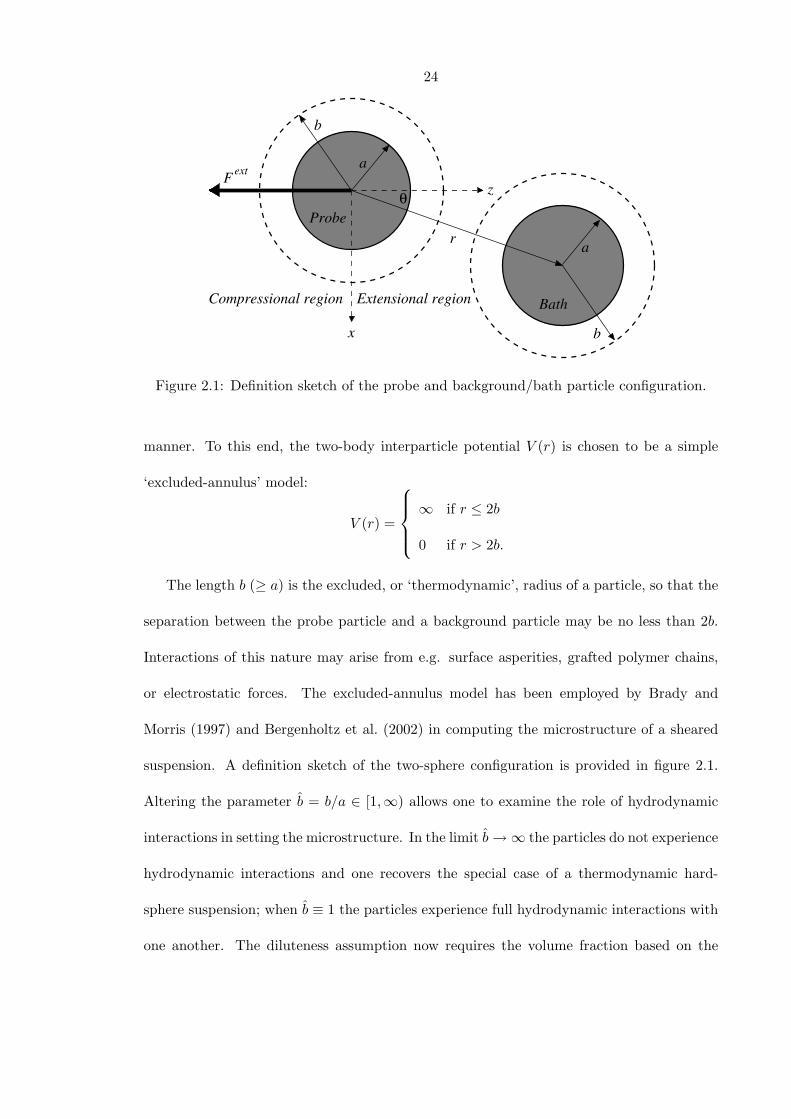
Figure 2.1: Definition sketch of the probe and background/bath particle configuration.

manner. To this end, the two-body interparticle potential V (r) is chosen to be a simple

‘excluded-annulus’ model:

V (r) =

∞ if r ≤ 2b

0 if r > 2b.

The length b (≥ a) is the excluded, or ‘thermodynamic’, radius of a particle, so that the

separation between the probe particle and a background particle may be no less than 2b.

Interactions of this nature may arise from e.g. surface asperities, grafted polymer chains,

or electrostatic forces. The excluded-annulus model has been employed by Brady and

Morris (1997) and Bergenholtz et al. (2002) in computing the microstructure of a sheared

suspension. A definition sketch of the two-sphere configuration is provided in figure 2.1.

Altering the parameter b = b/a ∈ [1,∞) allows one to examine the role of hydrodynamic

interactions in setting the microstructure. In the limit b→∞ the particles do not experience

hydrodynamic interactions and one recovers the special case of a thermodynamic hard-

sphere suspension; when b ≡ 1 the particles experience full hydrodynamic interactions with

one another. The diluteness assumption now requires the volume fraction based on the

25

excluded radius b to be small, φb = 4πnb3/3 1.

The pair-level Smoluchowski equation is made dimensionless by scaling quantities as

r ∼ b, U ∼ F0

6πηa, D ∼ 2D, and t ∼ 6πηab

F0,

where F0 is the magnitude of the external force F ext and D = kT/6πηa is the Stokes-

Einstein-Sutherland diffusivity of an isolated colloidal particle of radius a. In this study

we consider time independent microstructures for which the scaled pair-level Smoluchowski

equation reads

Peb∇ · (Ug) = ∇ ·D ·∇g, (2.2)

where all quantities are dimensionless, and for brevity the subscripts on ∇r,U r, and

Dr have been dropped. The above equation reflects the competition between advection due

to the application of an external force on the probe particle (the left-hand side of (2.2)) in

driving the system out of equilibrium and Brownian motion (the right-hand side of (2.2))

in attempting to restore equilibrium. The degree to which the microstructure is distorted

from its equilibrium state is governed by the Peclet number, Peb = F0/(2kT/b), which

emerges naturally from the scaling. The subscript b indicates that the Peclet number is

based on the excluded radius b rather than the hydrodynamic radius a. The Peclet number

may be viewed as a ratio of forces: the external force F0 over the Brownian force 2kT/b,

or alternatively, as a ratio of time scales: the diffusive time τD = b2/2D divided by the

advective time τA = 6πηab/F0. Either way, it should be clear that increasing the Peclet

number corresponds to driving the system away from equilibrium.

To fully determine the pair-distribution function the Smoluchowski equation (2.2) must

be accompanied by appropriate boundary conditions. It is assumed that the suspension

26

lacks any long-range order, which implies that

g(s) → 1 as s→∞, (2.3)

where s = r/b. The effect of the interparticle potential requires that the radial compo-

nent of the relative flux is zero at r = 2b; thus, we have

s ·D ·∇g = Peb s ·Ug at s = 2, (2.4)

with s = s/s the radial unit vector. As the pair-distribution function approaches unity

at large distances it is useful to define the structural deformation function f(s) ≡ g(s) −

1. Furthermore, in the dilute limit as the equilibrium pair-distribution function is unity

everywhere (i.e. for s ≥ 2), the structural deformation function is the departure from

equilibrium caused by application of the external force on the probe.

2.3 Average velocity of the probe particle and its interpre-

tation as a microviscosity

At low Reynolds number the average velocity of the probe particle may be written as

〈U〉 = U0 + 〈UH〉+ 〈UP 〉+ 〈UB〉, (2.5)

where U0 = F ext/6πηa is the velocity of the probe particle in isolation. The presence

of background colloidal particles causes the average velocity of the probe to differ from U0.

This difference may be expressed as the sum of hydrodynamic 〈UH〉, interparticle 〈UP 〉,

27

and Brownian 〈UB〉 contributions. In (2.5) the angle brackets denote an ensemble average

over the admissible positions of a background particle, and the overline on 〈UB〉 denotes an

average over the many collisions of the probe and background particles with the surrounding

solvent molecules. In this section we derive expressions for each of the three contributions.

The velocity of particle 1 (U1 say) subjected to an external force F 1 in the presence of

particle 2 subject to another external force F 2 is

U1 = MUF11 · F 1 + MUF

12 · F 2.

In the present case where the particles are spherical and of equal size the mobility tensors

take the form

MUFij =

16πηa

Aij(bs)ss +Bij(bs)(I − ss)

,

where I is the identity tensor, and Aij(r) and Bij(r) are scalar mobility functions

that depend on the magnitude of the dimensionless separation between the particles only.

Following the notation of Batchelor (1982), the relative Brownian diffusivity tensor and

relative velocity are given by

D = G(bs)ss +H(bs) (I − ss) , (2.6)

U =[G(bs)ss +H(bs) (I − ss)

]·(−F

ext),

where Fext

= F ext/F0. The absence of a factor of 2 multiplying the right hand side of

(2.6) is due to the relative diffusivity tensor being scaled with 2D (the relative diffusivity

of a pair of isolated spheres) rather than D (the Stokes-Einstein-Sutherland diffusivity of a

single isolated sphere). The hydrodynamic functions G(r) and H(r) describe the relative

28

mobility parallel and transverse to the line of centers of a pair of spheres respectively and

are defined by

G(r) = A11(r)−A12(r),

H(r) = B11(r)−B12(r).

The velocity of the probe particle caused by the application of the external force is

MUF11 · F ext; hence, the velocity due to hydrodynamic interactions is simply

UH =F ext

6πηa·A11(bs)ss +B11(bs)(I − ss)− I

,

i.e. the difference between the total velocity MUF11 · F ext and the velocity in isolation

U0. To obtain the average velocity due to hydrodynamic interactions the configuration-

specific velocity UH is weighted by the probability that the probe particle and a background

particle are in a configuration characterized by the vector separation s (namely ng(s)) and

averaged over the ensemble of all possible configurations. Following this program we have

〈UH〉 =3φb

4πF ext

6πηa·∫

s≥2

A11(bs)ss +B11(bs)(I − ss)− I

g(s)ds. (2.7)

It is important to note for large s that UH ∼ O(s−4) and g(s) ∼ O(1); thus, the integral

in (2.7) is convergent.

Suppose that the probe particle experiences an interparticle-force interaction with a

background particle specified by the interparticle force F P ; the average velocity of the

29

probe due to this interparticle force is given by

〈UP 〉 =1

6πηa3φb

4π

∫s≥2

G(bs)ss +H(bs)(I − ss)

· F P (s)g(s)ds.

The excluded-annulus model is represented by a hard-sphere force F P = −(kT/2b)δ(s−

2)s, where δ(x) is the Dirac delta distribution. Substituting this into the above equation

we have

〈UP 〉 = − F0

6πηa3φb

4π2G(2b)Peb

∮s=2

g(s)sdΩ. (2.8)

An immediate consequence of (2.8) is that in the limit b → 1, where G(2b) ∼ b − 1,

〈UP 〉 → 0. This is a statement of the fact that the hard-sphere force plays no dynamical

role in the case b ≡ 1: the rigidity of the particles is realized by the vanishing relative radial

mobility.

Lastly, we consider the average velocity contribution of the probe particle due to Brow-

nian motion. In appendix 2.A it is shown that

UB = −12∇ ·D, (2.9)

where the divergence is taken with respect to the last index of the relative diffusivity

tensor. Averaging (2.9) over the ensemble of admissible two-particle configurations yields

〈UB〉 = − F0

6πηa3φb

4π1

Peb

∫s≥2

(G(bs)−H(bs)

s+

12dG(bs)ds

)g(s)sds. (2.10)

The same result may be derived if one supposes the effect of Brownian motion is equiv-

alent to the action of equal and opposite ‘thermodynamic forces’ F B1 = kT∇ ln g(s) and

F B2 = −F B

1 acting on the probe and a background particle respectively (Batchelor 1982).

30

Note, the integrand in (2.10) is of O(s−5) for large s; hence, the integral is convergent.

Aside from the external force there are no other directional influences on g(s); therefore,

g(s) is axially-symmetric about the orientation of F ext. Moreover, as U0 is parallel to F ext

one expects 〈UH〉, 〈UP 〉, and 〈UB〉 to be parallel to F ext also. With this in mind, one is

able to interpret the change in translational velocity of the probe due to the presence of the

background particles as a dimensionless relative microviscosity, ηr, of the suspension. This

is done by application of the Stokes drag formula F ext/6πηa = ηr〈U〉. Thus, the relative

microviscosity is defined by

ηr ≡F0

6πηaFext · 〈U〉

. (2.11)

Note, the microviscosity contains (through its dependence on 〈U〉) an a priori unknown

dependence on the probe-to-background particle size ratio; this fact must be appreciated

when analyzing results from an active tracking experiment. In our study the probe and

background particles are of equal size so this is not a concern (see, however, the discussion

in § 2.7 and Squires and Brady 2005).

For dilute dispersions the denominator in (2.11) can be expanded to first order in the

background particle volume fraction φb, and the relative microviscosity may be written as

ηr = 1 + ηiφb, where ηi = ηHi + ηP

i + ηBi is the intrinsic microviscosity (i.e. the relative mi-

croviscosity minus the Newtonian solvent contribution and normalized by the background

particle volume fraction); ηHi , ηP

i , and ηBi are the hydrodynamic, interparticle, and Brow-

nian contributions to the intrinsic microviscosity, respectively. A question we shall explore

later is the relation between this microviscosity and the macroviscosity determined from

studies on macroscopically sheared colloidal dispersions.

To highlight the role played by the nonequilibrium microstructure it is instructive to

31

express the intrinsic microviscosity contributions in terms of the structural deformation

function f(s). Firstly, for the intrinsic hydrodynamic microviscosity we have

ηHi = ηH

i,0 −34π

Fext

Fext

:∫

s≥2

A11(bs)ss +B11(bs)(I − ss)− I

f(s)ds, (2.12)

where ηHi,0 is the contribution to the intrinsic hydrodynamic microviscosity due to the

equilibrium microstructure:

ηHi,0 = −

∫ ∞

2(A11(bs) + 2B11(bs)− 3)s2ds. (2.13)

The intrinsic interparticle microviscosity takes the form

ηPi =

34π

2G(bs)Peb

Fext ·

∮s=2

f(s)sdΩ, (2.14)

from which we see the equilibrium microstructure does not affect ηPi . For the intrinsic

Brownian microviscosity we have

ηBi =

34π

1Peb

Fext ·

∫s≥2

(G(bs)−H(bs)

s+

12dG(bs)ds

)f(s)s ds, (2.15)

which, as in the case of the intrinsic interparticle microviscosity, depends solely on the

nonequilibrium microstructure.

32

2.4 Nonequilibrium microstructure and microrheology at small

Peb

2.4.1 Perturbation expansion of the structural deformation

At small Peclet number, when the ratio of the external force to the restoring Brownian force

is much less than unity, the suspension is only slightly displaced from its equilibrium state,

enabling the pair-distribution function to be calculated via a perturbation expansion in Peb.

Recalling the definition of Peb as a ratio of timescales one anticipates that the perturbation

to the equilibrium microstructure is singular, based on the general non-uniformity criterion

proposed by Van Dyke (1975, pp. 80-83). Before dealing with the complicating effect of

hydrodynamic interactions it is useful to examine the singular nature of the problem in

their absence. Neglecting hydrodynamic interactions the pair-level Smoluchowski equation

(2.2) and associated boundary conditions (2.3) and (2.4) reduce to

PebU ·∇f = ∇2f, (2.16)

Peb(s · U)(1 + f) =df

dsat s = 2, (2.17)

f → 0 as s→∞, (2.18)

where U = −Fext

. The distortion to the equilibrium microstructure is governed by a

balance between isotropic diffusion and advection by a constant relative ‘velocity’ U . Even

though the Peclet number is small from (2.16) we see that at distances s ∼ O(Pe−1b ) (where

hydrodynamic interactions are unimportant anyway) the effects of advection and diffusion

are of the same order of magnitude. Defining an ‘outer’ coordinate ρ = sPeb ∼ O(1) we see

33

that (2.16) takes the form

U ·∇ρF = ∇2ρF, (2.19)

in this outer region; for clarity, we denote the structural deformation in the outer region

as F . It is required that a solution to (2.19) must vanish as ρ → ∞ and match with the

solution of the ‘inner’ equation (2.16) as ρ→ 0. If Peb ≡ 0 then the uniformly valid solution

is simply f = 0, corresponding to an equilibrium microstructure.

In the inner region the first perturbation to the equilibrium microstructure is linear in

the forcing U and is given by

f = −Peb4s2

s · U , (2.20)

which has the character of a diffusive dipole directed along Fext

. In terms of the outer

variables (2.20) is

f = −Pe3b

4ρ2

ρ · U ;

thus, the leading order perturbation to the equilibrium microstructure is of O(Pe3b) in

the outer region. This indicates that the expansion in the inner region will be regular

through terms of O(Pe2b); specifically, we may write

f = f1Peb + f2Pe2b +O(Pe3

b),

where f1 is given by (2.20). Now, f2 must be quadratic in the forcing U and it is a

simple (if tedious) matter to show that

f2 = 2(

4s3− 1s

)ss : UU − 2

(4

3s3− 1s

), (2.21)

34

from which it is seen that to leading order f2Pe2b ∼ O(Pe3

b) in the outer region also;

hence, the first term in the outer expansion should be matched to f1Peb + f2Pe2b . Now, if

one supposes the next term in the inner expansion to be f3Pe3b , then the singular nature of

the expansion is revealed, because the particular solution of f3 is forced by gradients in f2,

which from (2.21) are to leading order O(s−2). The resulting particular solution for f3 does

not decay as s → ∞. The matching condition for f3 is: f1Peb + f2Pe2b + f3Pe3

b = F1Pe3b

in the limits ρ→ 0 and s→∞, where F1 is the first term in the outer solution. Although

one may continue to higher orders in the expansion, the system (2.16)-(2.18) can be solved

exactly (Squires and Brady 2005), making this unnecessary.

We now consider the effect of hydrodynamic interactions. Guided by the analysis above

we propose an expansion for the structural deformation in the inner region of the form

f = Pebs · Fextf1(s) + Pe2

b

(ss : F

extF

extf2(s) + h2(s)

)+O(Pe3

b). (2.22)

Substituting this expansion into the Smoluchowski equation (2.2) and boundary condi-

tions (2.3) and (2.4) one obtains at O(Peb) the system

d

ds

(s2G(bs)

df1

ds

)− 2H(bs)f1 = −s2W (bs), (2.23)

df1

ds= −1 at s = 2,

f1 → 0 as s→∞,

where W (r) = dG/dr + 2(G − H)/r, is proportional to the divergence of the relative

35

2 2.5 3 3.5 4 4.5 50

0.2

0.4

0.6

0.8

1

s

f 1

10−3 10−2 10−1 100 101 1020.50.60.70.80.91

b/a −1

f 1(2)

∞3

1.5 1.1

b/a = 1.001

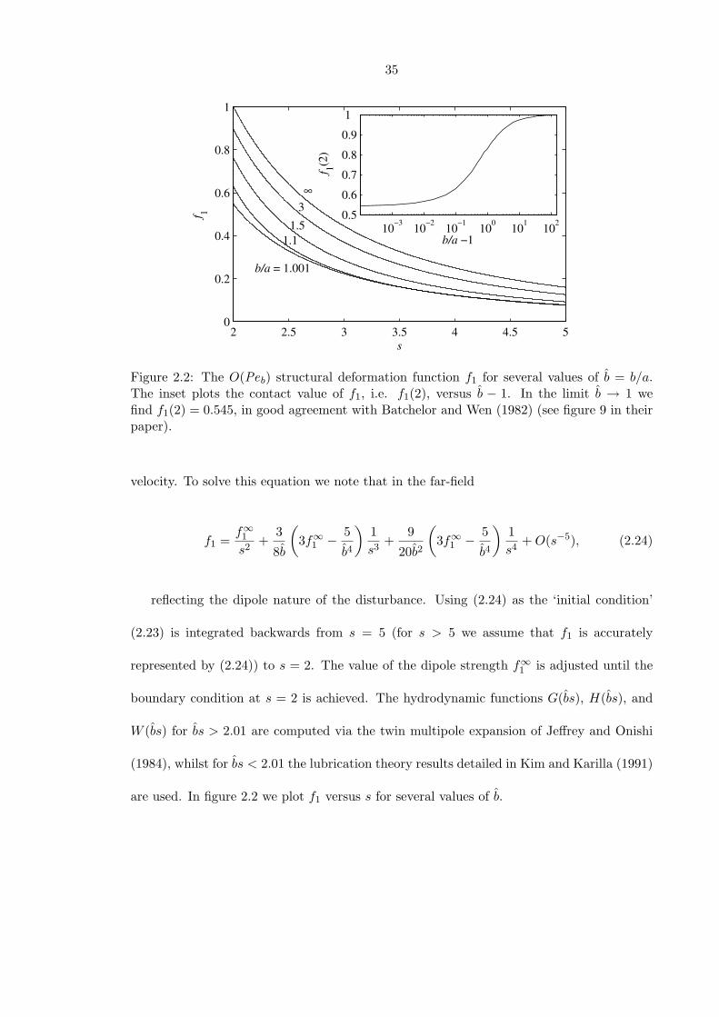
Figure 2.2: The O(Peb) structural deformation function f1 for several values of b = b/a.The inset plots the contact value of f1, i.e. f1(2), versus b − 1. In the limit b → 1 wefind f1(2) = 0.545, in good agreement with Batchelor and Wen (1982) (see figure 9 in theirpaper).

velocity. To solve this equation we note that in the far-field

f1 =f∞1s2

+3

8b

(3f∞1 − 5

b4

)1s3

+9

20b2

(3f∞1 − 5

b4

)1s4

+O(s−5), (2.24)

reflecting the dipole nature of the disturbance. Using (2.24) as the ‘initial condition’

(2.23) is integrated backwards from s = 5 (for s > 5 we assume that f1 is accurately

represented by (2.24)) to s = 2. The value of the dipole strength f∞1 is adjusted until the

boundary condition at s = 2 is achieved. The hydrodynamic functions G(bs), H(bs), and

W (bs) for bs > 2.01 are computed via the twin multipole expansion of Jeffrey and Onishi

(1984), whilst for bs < 2.01 the lubrication theory results detailed in Kim and Karilla (1991)

are used. In figure 2.2 we plot f1 versus s for several values of b.

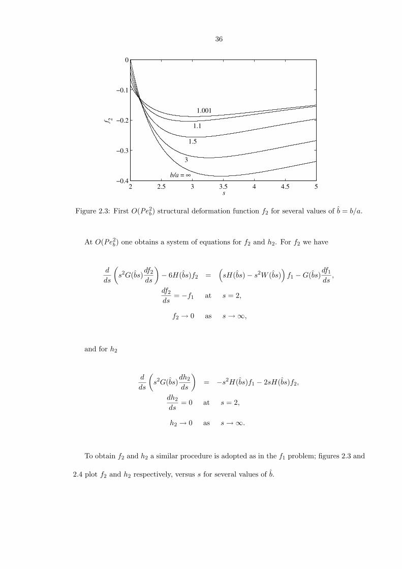
36

2 2.5 3 3.5 4 4.5 5−0.4

−0.3

−0.2

−0.1

0

s

f 2

b/a = ∞

3

1.5

1.1

1.001

Figure 2.3: First O(Pe2b) structural deformation function f2 for several values of b = b/a.

At O(Pe2b) one obtains a system of equations for f2 and h2. For f2 we have

d

ds

(s2G(bs)

df2

ds

)− 6H(bs)f2 =

(sH(bs)− s2W (bs)

)f1 −G(bs)

df1

ds,

df2

ds= −f1 at s = 2,

f2 → 0 as s→∞,

and for h2

d

ds

(s2G(bs)

dh2

ds

)= −s2H(bs)f1 − 2sH(bs)f2,

dh2

ds= 0 at s = 2,

h2 → 0 as s→∞.

To obtain f2 and h2 a similar procedure is adopted as in the f1 problem; figures 2.3 and

2.4 plot f2 and h2 respectively, versus s for several values of b.

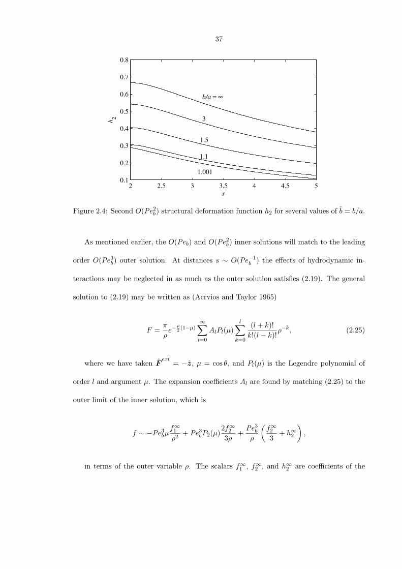
37

2 2.5 3 3.5 4 4.5 50.1

0.2

0.3

0.4

0.5

0.6

0.7

0.8

s

h 2

b/a = ∞

3

1.5

1.1

1.001

Figure 2.4: Second O(Pe2b) structural deformation function h2 for several values of b = b/a.

As mentioned earlier, the O(Peb) and O(Pe2b) inner solutions will match to the leading

order O(Pe3b) outer solution. At distances s ∼ O(Pe−1

b ) the effects of hydrodynamic in-

teractions may be neglected in as much as the outer solution satisfies (2.19). The general

solution to (2.19) may be written as (Acrvios and Taylor 1965)

F =π

ρe−

ρ2(1−µ)

∞∑l=0

AlPl(µ)l∑

k=0

(l + k)!k!(l − k)!

ρ−k, (2.25)

where we have taken Fext

= −z, µ = cos θ, and Pl(µ) is the Legendre polynomial of

order l and argument µ. The expansion coefficients Al are found by matching (2.25) to the

outer limit of the inner solution, which is

f ∼ −Pe3bµf∞1ρ2

+ Pe3bP2(µ)

2f∞23ρ

+Pe3

b

ρ

(f∞23

+ h∞2

),

in terms of the outer variable ρ. The scalars f∞1 , f∞2 , and h∞2 are coefficients of the

38

leading order terms of f1, f2, and h2 respectively as s → ∞; hence, the outer solution is

indirectly influenced by hydrodynamic interactions. Matching inner and outer solutions one

finds that

A0 = Pe3b

h∞2π, A1 = −Pe3

b

f∞12π

, Al = 0 ∀ l > 1,

so that the outer solution to leading order is

F =Pe3

b

ρe−

ρ2(1−µ)

h∞2 + µf∞2

(1 +

2ρ

),

which is basically the Green’s function for (2.19) with an additional term (proportional

to f∞2 ) accounting for the dipole structure of the leading order inner solution. Physically,

on the scale of ρ the probe appears to be a point source of structural deformation. At large

distances (s ∼ O(Pe−1b )) the perturbation to the equilibrium microstructure produced by

this point source is exponentially small everywhere except in a wake region where ρ(1−µ) ∼

O(1) in which the decay is algebraic ∼ ρ−1. In the limit ρ → ∞ the area of non-zero

structural deformation is restricted to θ ∼ O(ρ−1/2).

2.4.2 Linear response: The intrinsic microviscosity and its relation to

self-diffusivity

Having analyzed the perturbation to the equilibrium microstructure we now proceed to

compute the resulting intrinsic microviscosity. Firstly, we shall consider small departures

from equilibrium, the so-called linear-response regime, where to O(Peb) the distortion of the

equilibrium microstructure is linearly related to the external force. This is the realm of pas-

sive microrheology. In addition to providing a valuable check of our numerical calculations,

one can relate the intrinsic microviscosity in this limit to the long-time self-diffusivity.

39

There are three translational diffusive processes occurring in colloidal dispersions; each

characterized with it’s own diffusivity: the short-time self-diffusivity Ds0; the long-time self-

diffusivity Ds∞; and the collective, or down-gradient, diffusivity Dc. For an isolated colloidal

particle all three diffusivities are identical and equal to the Stokes-Einstein-Sutherland dif-

fusivity D = kT/6πηa. However, at finite particle concentrations the three diffusivities are

different and correspond to distinct physical processes. BothDs0 andDs

∞ are concerned with

the diffusion of a single test particle in a macroscopically quiescent dispersion (although on

quite different timescales), whilst Dc is the constant of proportionality relating the flux of

particles down a steady small concentration gradient (see e.g. Batchelor 1976).

The short-time self-diffusivity measures the instantaneous, or local, mobility of a par-

ticle on a time interval which is large compared to the inertial, or momentum, relaxation

timescale of the particle tI = m/6πηa (where m is the mass of the particle) but small

compared to the diffusive timescale of the particle tD = a2/D. Within this time interval

the particle will have experienced many collisions from the surrounding solvent molecules

without moving an appreciable fraction of its size and hence without affecting the spatial

arrangement of the particles surrounding it. Thus, one defines the short-time self-diffusivity

as the ensemble average of the particle mobility with respect to the equilibrium configuration

of the dispersion. If the test particle experiences hydrodynamic interactions with surround-

ing particles its mobility will be decreased from its value at infinite dilution; therefore,

the short-time self-diffusivity is less than the Stokes-Einstein-Sutherland diffusivity. The

difference between the short-time self-diffusivity and the Stokes-Einstein-Sutherland diffu-

sivity is nothing but the equilibrium hydrodynamic microviscosity ηHi,0, defined in (2.13)

as the ensemble average of the probe particle’s mobility with respect to the equilibrium

40

pair-distribution function. Indeed, one may make the formal relationship

Ds0

D= 1− ηH

i,0φb,

correct to first order in φb (There is also a direct relation between Ds0 and ηH

i,0 valid for

all φb, Brady 1994).

To examine the effects of hydrodynamic interactions onDs0 we may view ηH

i,0 as a function

of the excluded radius b. In the limit of long-range excluded volume interactions (b 1)

the asymptotic formulas for A11 and B11 (see e.g. Kim and Karilla 1991) may be used to

show

ηHi,0 =

15

8b4− 9

64b6− 1

20b8+

737

7168b10+O(b−12). (2.26)

For general values of b one must evaluate ηHi,0 numerically. This is accomplished by

splitting the range of integration [2,∞) into three regions: 2 ≤ bs < 2.01, in which the

contribution to the integral is evaluated analytically using lubrication theory results for the

hydrodynamic functions; 2.01 ≤ bs < 3, where the hydrodynamic functions are obtained

via a twin multipole expansion (Jeffrey and Onishi 1984) and the integral is performed

numerically; and 3 ≤ bs <∞, where the far-field forms of the hydrodynamic functions are

used. In figure 2.5 we plot ηHi,0 as a function of b; the solid line in figure 2.5 is the first

term in the series (2.26), whilst the circles represent the full numerical evaluation. The

agreement between the two is excellent. For the case of full hydrodynamic interactions

(b = 1) we find ηHi,0 = 1.83 in agreement with Batchelor (1976). Note, the first term in the

series (2.26) gives a value of ηHi,0 = 1.875 for b = 1, which is remarkably close to the actual

value. As ηHi,0 is positive the effect of hydrodynamic interactions is to decrease Ds

0/D, as

the motion of the probe is hindered by hydrodynamic interactions with its neighbors. Of

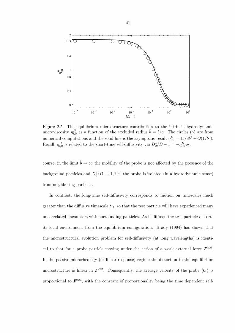
41

10−5 10−4 10−3 10−2 10−1 100 101

0

0.4

0.8

1

1.4

1.83

2

b/a − 1

ηH i,0

Figure 2.5: The equilibrium microstructure contribution to the intrinsic hydrodynamicmicroviscosity ηH

i,0 as a function of the excluded radius b = b/a. The circles () are fromnumerical computations and the solid line is the asymptotic result ηH

i,0 = 15/8b4 +O(1/b6).Recall, ηH

i,0 is related to the short-time self-diffusivity via Ds0/D − 1 = −ηH

i,0φb.

course, in the limit b→∞ the mobility of the probe is not affected by the presence of the

background particles and Ds0/D → 1, i.e. the probe is isolated (in a hydrodynamic sense)

from neighboring particles.

In contrast, the long-time self-diffusivity corresponds to motion on timescales much

greater than the diffusive timescale tD, so that the test particle will have experienced many

uncorrelated encounters with surrounding particles. As it diffuses the test particle distorts

its local environment from the equilibrium configuration. Brady (1994) has shown that

the microstructural evolution problem for self-diffusivity (at long wavelengths) is identi-

cal to that for a probe particle moving under the action of a weak external force F ext.

In the passive-microrheology (or linear-response) regime the distortion to the equilibrium

microstructure is linear in F ext. Consequently, the average velocity of the probe 〈U〉 is

proportional to F ext, with the constant of proportionality being the time dependent self-

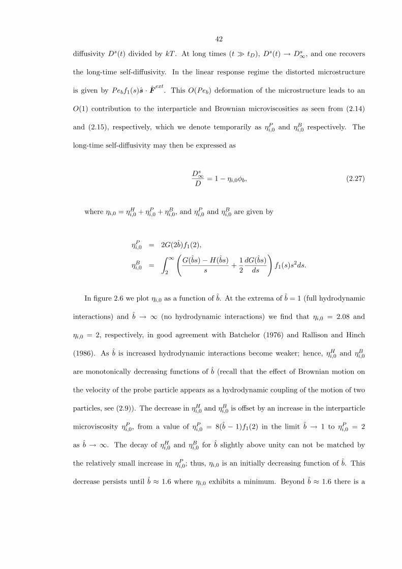
42

diffusivity Ds(t) divided by kT . At long times (t tD), Ds(t) → Ds∞, and one recovers

the long-time self-diffusivity. In the linear response regime the distorted microstructure

is given by Pebf1(s)s · Fext

. This O(Peb) deformation of the microstructure leads to an

O(1) contribution to the interparticle and Brownian microviscosities as seen from (2.14)

and (2.15), respectively, which we denote temporarily as ηPi,0 and ηB

i,0 respectively. The

long-time self-diffusivity may then be expressed as

Ds∞D

= 1− ηi,0φb, (2.27)

where ηi,0 = ηHi,0 + ηP

i,0 + ηBi,0, and ηP

i,0 and ηBi,0 are given by

ηPi,0 = 2G(2b)f1(2),

ηBi,0 =

∫ ∞

2

(G(bs)−H(bs)

s+

12dG(bs)ds

)f1(s)s2ds.

In figure 2.6 we plot ηi,0 as a function of b. At the extrema of b = 1 (full hydrodynamic

interactions) and b → ∞ (no hydrodynamic interactions) we find that ηi,0 = 2.08 and

ηi,0 = 2, respectively, in good agreement with Batchelor (1976) and Rallison and Hinch

(1986). As b is increased hydrodynamic interactions become weaker; hence, ηHi,0 and ηB

i,0

are monotonically decreasing functions of b (recall that the effect of Brownian motion on

the velocity of the probe particle appears as a hydrodynamic coupling of the motion of two

particles, see (2.9)). The decrease in ηHi,0 and ηB

i,0 is offset by an increase in the interparticle

microviscosity ηPi,0, from a value of ηP

i,0 = 8(b − 1)f1(2) in the limit b → 1 to ηPi,0 = 2

as b → ∞. The decay of ηHi,0 and ηB

i,0 for b slightly above unity can not be matched by

the relatively small increase in ηPi,0; thus, ηi,0 is an initially decreasing function of b. This

decrease persists until b ≈ 1.6 where ηi,0 exhibits a minimum. Beyond b ≈ 1.6 there is a

43

10−3 10−2 10−1 100 101 102

0

0.25

0.5

0.75

1

1.25

1.5

1.75

2 2.1

b/a − 1

η i,0

Figure 2.6: Intrinsic microviscosity contributions in the limit Peb → 0 as a function ofb = b/a: , total (ηi,0); , hydrodynamic (ηH

i,0); , Brownian (ηBi,0); and 4, interparticle

force (ηPi,0). Recall, ηi,0 is related to the long-time self-diffusivity via Ds

∞/D − 1 = −ηi,0φb.

monotonic increase of ηi,0 to its limiting value of 2 as b→∞.

The nonmonotonicity of ηi,0 is somewhat surprising and suggests the intriguing possi-

bility of maximizing the long-time self-diffusivity of a particle through modulation of its

interparticle-force interactions. If the volume fraction in (2.27) were based on the hydro-

dynamic radius a instead of the thermodynamic radius b (note that φb = b3φa) one must

multiply ηi,0 by b3, implying that the long-time self-diffusivity decreases monotonically

(and without bound) with increasing b. However, the geometric, or excluded, radius b is

the correct length scale in defining the volume fraction, as particles must actually move

past each other on this scale. The maximum in the long-time self-diffusivity (at b ≈ 1.6)

arises because b is sufficiently greater than unity, so that the highly resistive hydrodynamic

lubrication interactions do not hinder the motion of the probe, while b is not too large,

whence the long-time self-diffusivity decreases due to the increased role of the hard sphere

44

interparticle-force. Although the values of long-time self-diffusivity at the extrema of b = 1

and b→∞ are similar, it is interesting to contrast the physical mechanisms at work in both

limits: for b = 1 the resistance to the probe motion is via hydrodynamic interactions with

other particles, which are mediated through the solvent fluid, whilst in the limit b→∞ the

probe motion is hindered by the excluded volume interparticle-force, which acts at contact

to provide a purely geometric resistance to the probe motion.

2.4.3 Weakly nonlinear theory

Our discussion of the intrinsic microviscosity and its relation to self-diffusivity took place in

the regime of linear response, where the departure from the equilibrium microstructure is

small and linearly related to the external force and Peb. The linear relationship between the

distorted microstructure and the external force manifests itself in the structural deformation

being fore-aft symmetric about the direction of the external force. Upon increasing Peb one

enters the nonlinear regime where the distortion to the equilibrium microstructure is no

longer linearly related to Peb, and the fore-aft symmetry of the structural deformation about

the external force is broken. The first nonlinear contribution to the structural deformation

(in the inner region) occurs at O(Pe2b) and was calculated in § 2.4.1. Here, we compute the

effect on the intrinsic microviscosity arising from this O(Pe2b) nonlinear deformation.

Firstly, it is readily seen from (2.22) and the symmetry of the integrals in (2.14) and

(2.15) that the O(Pe2b) structural deformation does not contribute to the Brownian and

interparticle microviscosities; however, there is a contribution to the hydrodynamic micro-

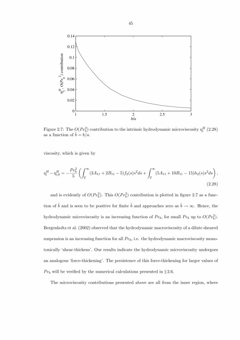
45

1 1.5 2 2.5 30

0.02

0.04

0.06

0.08

0.1

0.12

0.14

b/a

η iH, O

(Pe b2 ) c

ontri

butio

n

Figure 2.7: The O(Pe2b) contribution to the intrinsic hydrodynamic microviscosity ηH

i (2.28)as a function of b = b/a.

viscosity, which is given by

ηHi −ηH

i,0 = −Pe2b

5

(∫ ∞

2(3A11 + 2B11 − 5)f2(s)s2ds+

∫ ∞

2(5A11 + 10B11 − 15)h2(s)s2ds

),

(2.28)

and is evidently of O(Pe2b). This O(Pe2

b) contribution is plotted in figure 2.7 as a func-

tion of b and is seen to be positive for finite b and approaches zero as b → ∞. Hence, the

hydrodynamic microviscosity is an increasing function of Peb, for small Peb up to O(Pe2b).

Bergenholtz et al. (2002) observed that the hydrodynamic macroviscosity of a dilute sheared

suspension is an increasing function for all Peb, i.e. the hydrodynamic macroviscosity mono-

tonically ‘shear-thickens’. Our results indicate the hydrodynamic microviscosity undergoes

an analogous ‘force-thickening’. The persistence of this force-thickening for larger values of

Peb will be verified by the numerical calculations presented in § 2.6.

The microviscosity contributions presented above are all from the inner region, where

46

s ∼ O(1), and we must also consider the magnitude of the contributions arising from the

outer region, where s ∼ O(ρPe−1b ). At large distances the nonequilibrium contribution to

the hydrodynamic microviscosity behaves as

ηHi − ηH

i,0 ∼∫

1s4fs2ds ∼ O(Pe4

b),

since f ∼ O(Pe3b) in the outer region. Hence, the O(Pe2

b) contribution to ηHi comes

exclusively from the inner region. Similarly, the outer contribution to the Brownian micro-

viscosity is

ηBi ∼ 1

Peb

∫1s5fs2ds ∼ O(Pe4

b).

However, the next term in the inner solution, Pe3bf3, will generate an O(Pe2

b) contribu-

tion to ηBi (and to ηP

i ) and is therefore of lower order than the O(Pe4b) contribution from

the leading order outer solution.

2.5 Numerical solution of the Smoluchowski equation for ar-

bitrary Peb

The perturbation analysis presented above sheds light on the microstructural deformation

in the case of small departures from equilibrium. Attempting to continue the expansion

to higher orders in Peb is unwise as the matching of inner and outer solutions must be

performed numerically (except in the absence of hydrodynamic interactions where it can be

done analytically) and the algebra involved becomes rapidly intractable. Thus, to obtain

the microstructure for arbitrary values of Peb one must solve the Smoluchowski equation

numerically. For Peb ∼ O(1) and higher this is a challenging task owing to the formation of

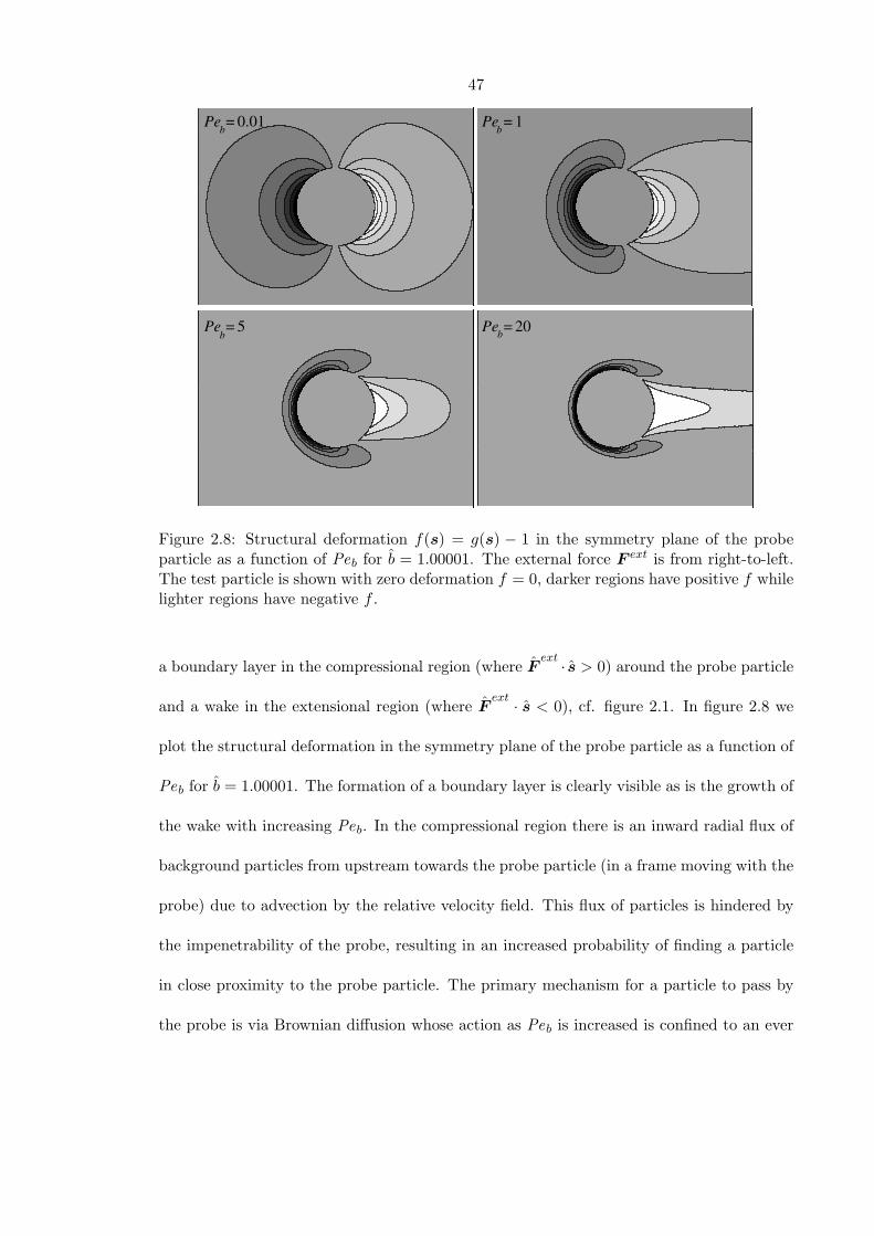
47

Pe =1

Pe =5 Pe =20

Pe =0.01

b b

b b

Figure 2.8: Structural deformation f(s) = g(s) − 1 in the symmetry plane of the probeparticle as a function of Peb for b = 1.00001. The external force F ext is from right-to-left.The test particle is shown with zero deformation f = 0, darker regions have positive f whilelighter regions have negative f .

a boundary layer in the compressional region (where Fext · s > 0) around the probe particle

and a wake in the extensional region (where Fext · s < 0), cf. figure 2.1. In figure 2.8 we

plot the structural deformation in the symmetry plane of the probe particle as a function of

Peb for b = 1.00001. The formation of a boundary layer is clearly visible as is the growth of

the wake with increasing Peb. In the compressional region there is an inward radial flux of

background particles from upstream towards the probe particle (in a frame moving with the

probe) due to advection by the relative velocity field. This flux of particles is hindered by

the impenetrability of the probe, resulting in an increased probability of finding a particle

in close proximity to the probe particle. The primary mechanism for a particle to pass by

the probe is via Brownian diffusion whose action as Peb is increased is confined to an ever

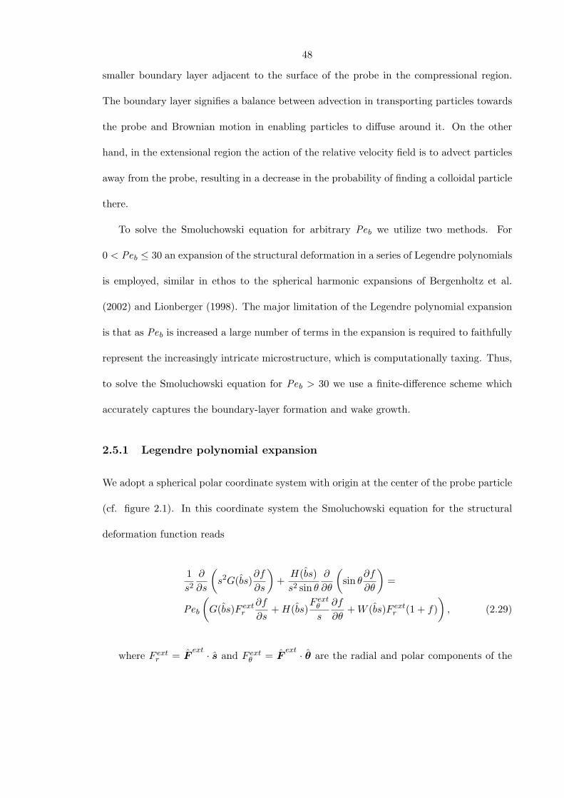
48

smaller boundary layer adjacent to the surface of the probe in the compressional region.

The boundary layer signifies a balance between advection in transporting particles towards

the probe and Brownian motion in enabling particles to diffuse around it. On the other

hand, in the extensional region the action of the relative velocity field is to advect particles

away from the probe, resulting in a decrease in the probability of finding a colloidal particle

there.

To solve the Smoluchowski equation for arbitrary Peb we utilize two methods. For

0 < Peb ≤ 30 an expansion of the structural deformation in a series of Legendre polynomials

is employed, similar in ethos to the spherical harmonic expansions of Bergenholtz et al.

(2002) and Lionberger (1998). The major limitation of the Legendre polynomial expansion

is that as Peb is increased a large number of terms in the expansion is required to faithfully

represent the increasingly intricate microstructure, which is computationally taxing. Thus,

to solve the Smoluchowski equation for Peb > 30 we use a finite-difference scheme which

accurately captures the boundary-layer formation and wake growth.

2.5.1 Legendre polynomial expansion

We adopt a spherical polar coordinate system with origin at the center of the probe particle

(cf. figure 2.1). In this coordinate system the Smoluchowski equation for the structural

deformation function reads

1s2

∂

∂s

(s2G(bs)

∂f

∂s

)+H(bs)s2 sin θ

∂

∂θ

(sin θ

∂f

∂θ

)=

Peb

(G(bs)F ext

r

∂f

∂s+H(bs)

F extθ

s

∂f

∂θ+W (bs)F ext

r (1 + f)), (2.29)

where F extr = F

ext · s and F extθ = F

ext · θ are the radial and polar components of the

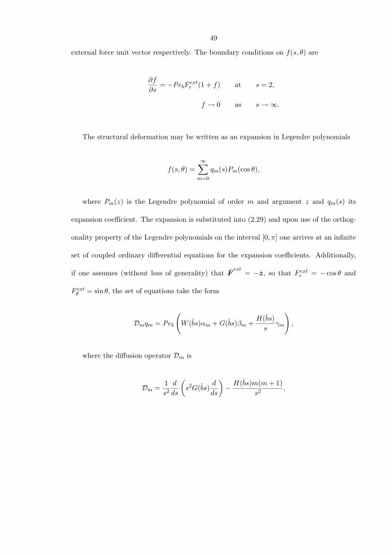
49

external force unit vector respectively. The boundary conditions on f(s, θ) are

∂f

∂s= −PebF

extr (1 + f) at s = 2,

f → 0 as s→∞.

The structural deformation may be written as an expansion in Legendre polynomials

f(s, θ) =∞∑

m=0

qm(s)Pm(cos θ),

where Pm(z) is the Legendre polynomial of order m and argument z and qm(s) its

expansion coefficient. The expansion is substituted into (2.29) and upon use of the orthog-

onality property of the Legendre polynomials on the interval [0, π] one arrives at an infinite

set of coupled ordinary differential equations for the expansion coefficients. Additionally,

if one assumes (without loss of generality) that Fext

= −z, so that F extr = − cos θ and

F extθ = sin θ, the set of equations take the form

Dmqm = Peb

(W (bs)αm +G(bs)βm +

H(bs)s

γm

),

where the diffusion operator Dm is

Dm =1s2

d

ds

(s2G(bs)

d

ds

)− H(bs)m(m+ 1)

s2,

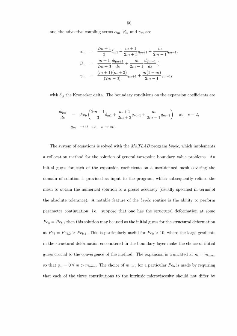
50

and the advective coupling terms αm, βm and γm are

αm =2m+ 1

3δm1 +

m+ 12m+ 3

qm+1 +m

2m− 1qm−1,

βm =m+ 12m+ 3

dqm+1

ds+

m

2m− 1dqm−1

ds, ]

γm =(m+ 1)(m+ 2)

(2m+ 3)qm+1 +

m(1−m)2m− 1

qm−1,

with δij the Kronecker delta. The boundary conditions on the expansion coefficients are

dqmds

= Peb

(2m+ 1

3δm1 +

m+ 12m+ 3

qm+1 +m

2m− 1qm−1

)at s = 2,

qm → 0 as s→∞.

The system of equations is solved with the MATLAB program bvp4c, which implements

a collocation method for the solution of general two-point boundary value problems. An

initial guess for each of the expansion coefficients on a user-defined mesh covering the

domain of solution is provided as input to the program, which subsequently refines the

mesh to obtain the numerical solution to a preset accuracy (usually specified in terms of

the absolute tolerance). A notable feature of the bvp4c routine is the ability to perform

parameter continuation, i.e. suppose that one has the structural deformation at some

Peb = Peb,1 then this solution may be used as the initial guess for the structural deformation

at Peb = Peb,2 > Peb,1. This is particularly useful for Peb > 10, where the large gradients

in the structural deformation encountered in the boundary layer make the choice of initial

guess crucial to the convergence of the method. The expansion is truncated at m = mmax

so that qm = 0 ∀ m > mmax. The choice of mmax for a particular Peb is made by requiring

that each of the three contributions to the intrinsic microviscosity should not differ by

51

more than 0.1% when computed using mmax and mmax+1 terms. As Peb increases so

does mmax, reflecting the need for more terms in the expansion to accurately describe the

microstructure. The highest value of Peb for which a solution was obtained was Peb = 30

requiring mmax = 60.

Finally, some care needs to be taken in application of the far-field boundary condition.

Here, we make the simple approximation of moving the boundary condition at infinity to

a finite radial location s = sfar, taking great care to ensure the choice of sfar does not

affect the computed intrinsic microviscosity contributions. For Peb < 1 at radial distances

O(Pe−1b ) advection is comparable to diffusion, requiring sfar O(Pe−1

b ). As a starting

point sfar is chosen to be 103Pe−1b and increased until convergence of each of the intrinsic

microviscosity contributions to eight decimal places is achieved. For Peb > 1, where, in

addition to the boundary-layer structure at the front of the probe, one must also account

for the wake region behind it (whose characteristic length grows linearly with Peb), we

start with sfar = 102Peb and increase sfar until the intrinsic microviscosity contributions

converge. In § 2.6 several studies are presented that validate our approximation of the

far-field boundary condition and demonstrate the accuracy of the numerical solutions.

2.5.2 Finite difference methods

Numerically solving the Smoluchowski equation accurately at large Peb is a demanding task:

the challenge is to capture the detailed boundary-layer structure of the pair-distribution

function near contact whilst maintaining sufficient resolution in the far-field to represent

the growing wake region behind the probe. In the range 2 ≤ Peb ≤ 100 the Smoluchowski

equation (2.29) is approximated by a finite difference equation, on a two-dimensional grid,

which has a dense collection of nodes in the boundary layer (to capture the large gradients

52

in the pair-distribution function there) and nodes distributed sparsely in the far-field. Both

radial and angular derivatives are approximated via central differences. Discretization of the

Smoluchowski equation leads to the linear matrix equation A ·f = w, where the coefficient

matrix A is tridiagonal with two fringes, f is the unknown structural deformation vector,

and w is the forcing vector. The matrix equation is solved iteratively using a simple Jacobi

scheme, requiring computation of the inverse of the tridiagonal portion of A, which is

performed via a standard back-substitution algorithm (Press et al. 1992). The method is

efficient in the sense that only the inverse of a tridiagonal matrix is to be computed, but

inefficient (as compared to other iterative techniques such as Gauss-Seidel or SOR) as it

requires a large number of iterations to converge. To reduce the number of iterations we

employ the convergence acceleration scheme proposed by Ng (1974). A detailed exposition

of the finite difference method is provided in appendix 2.B.

As Peb is increased one requires a greater number of grid points (and hence iterations)

for the method to converge. Beyond Peb ≈ 100 the iteration diverges; at such large Peb it is

reasonable to postulate that the rheological properties of the suspension are primarily de-

termined by the large gradients in the pair-distribution function occurring in the boundary

layer. Thus, for Peb > 100 we solve a boundary-layer approximation to the full Smolu-

chowski equation, which is derived in appendix 2.C. This equation retains the information

on the detailed structure of the boundary layer at the expense of obtaining accurate far-field

behavior. The boundary-layer equation reads

G∂2f

∂y2+Q

∂f

∂y+

Pe−2b H

4 sin θ∂

∂θ

(sin θ

∂f

∂θ

)= Pe−1

b

(W cos θ(1 + f)− H

2sin θ

∂f

∂θ

), (2.30)

where y = Peb(s−2) is a stretched radial coordinate, Q = −G cos θ+dG/dy+Pe−1b G(1−

53

Pe−1b y/2), and terms of O(Pe−3

b ) and greater have been discarded. The crucial distinction

between (2.30) and the full Smoluchowski equation (2.29) is the absence of the 1/s2 factor

multiplying the diffusive terms on the left-hand side of (2.30). This results in the exaggera-

tion of diffusive effects at large s. Consequently, although there remains a wake behind the

probe particle its size is diminished, making numerical solution of (2.30) considerably easier

than that of (2.29). Strictly speaking, the structural deformation determined from (2.30)

should be matched to an outer solution from the advectively dominated region. However,

this is not a simple task as the radial matching length is a function of the polar angle θ.

Here, we assume that the solution of (2.30) is valid throughout the entire domain, specif-

ically requiring that the solution should vanish at large radial separations. To solve the

boundary-layer equation we use a finite difference method analogous to that employed for

solution of the full Smoluchowski equation.

2.6 Results

2.6.1 No hydrodynamic interactions

In this subsection the microstructure and microviscosity of the dispersion are examined in

the absence of hydrodynamic interactions, b→∞. Particular attention is paid to this limit

as the accuracy of our numerical calculations may be demonstrated via comparison to the

exact solution of the Smoluchowski equation derived by Squires and Brady (2005) and the

perturbation analysis of § 2.4.

For weak forcing it was shown in § 2.4 that to O(Pe2b) the contact value of the structural

54

00.1

0.2

0.3

0.4

0.5

0.6

2/3

θ

(f −

Pebf 1) /

Pe b2

π/4 π/2 3π/4 π

Figure 2.9: Angular dependence of the structural deformation at contact (s = 2) for sev-eral Peb in the absence of hydrodynamic interactions: Peb = 10−3 (); Peb = 10−2 ();Peb = 10−1 (); and Peb = 1 (4). The solid line is the O(Pe2

b) perturbation result(f − Pebf1)/Pe2

b = 2/3 +O(Peb).

deformation is

f(2, θ) = −Peb cos θf1(2) + Pe2b

(cos2 θf2(2) + h2(2)

), (2.31)

where for definiteness it is assumed Fext

= −z. Figure 2.9 compares the contact value

obtained via the Legendre polynomial expansion to the perturbation theory result. In figure

2.9 the O(Pe2b) term has been isolated by plotting (f(2, θ) + Peb cos θ)/Pe2

b versus Peb and

comparing to the perturbation result 2/3+O(Peb). Evidently, the numerical calculations are

in good agreement with the perturbation theory up to Peb = 0.1, beyond which one requires

higher order terms in the expansion (2.31) to accurately represent the microstructure.

We now turn our attention to the structural deformation at large Peb, which is computed

via a finite difference solution of the full Smoluchowski equation (2 ≤ Peb ≤ 100) and a

55

boundary-layer approximation of it (20 ≤ Peb ≤ 1000). In the absence of hydrodynamic

interactions there is no reduction in the relative mobility as a force-free particle approaches

the probe particle. Thus, at large Peb the strong inward advective flux of force-free particles

(in a reference frame moving with the probe) in the compressional region (upstream) leads

to a large accumulation of pair density in a boundary layer at the surface of the probe

particle. The probe acts as an obstruction around which the force-free particles coming

from upstream must pass. The primary mechanism of passing is via Brownian diffusion,

which is driven by the large gradients of pair-density present in the boundary layer. In the

extensional region (downstream) advection carries the force-free particles away from the

probe and a decrease in pair density, or wake, resides there. In appendix 2.D we show that

at large Peb the pair-distribution function is given by

g(s, θ) =

F ext

r Peb exp−F ext

r Peb(s− 2)

+O(1) if F extr ≥ 0

0 if F extr < 0

(2.32)

The contact value of the pair-distribution function in the compressional region, g(2) =

F extr Peb, scales linearly with Peb. In figure 2.10 we plot the contact value as a function of

the polar angle θ for several Peb. The inset shows that scaling g(2) with Peb collapses that

data well, verifying the linear scaling predicted by (2.32).

In the absence of hydrodynamic interactions the intrinsic microviscosity of the suspen-

sion, ηi, is determined solely by the interparticle-force contribution (2.14), which is propor-

tional to the contact value of the structural deformation. Figure 2.11 plots ηi as a function

of Peb. In the limit Peb → 0, where the structural deformation is linear in the external

force, there is a Newtonian plateau at which ηi = 2. On increasing Peb the non-Newtonian

character of the dispersion is evident in the decrease, or force-thinning, of ηi. The inset

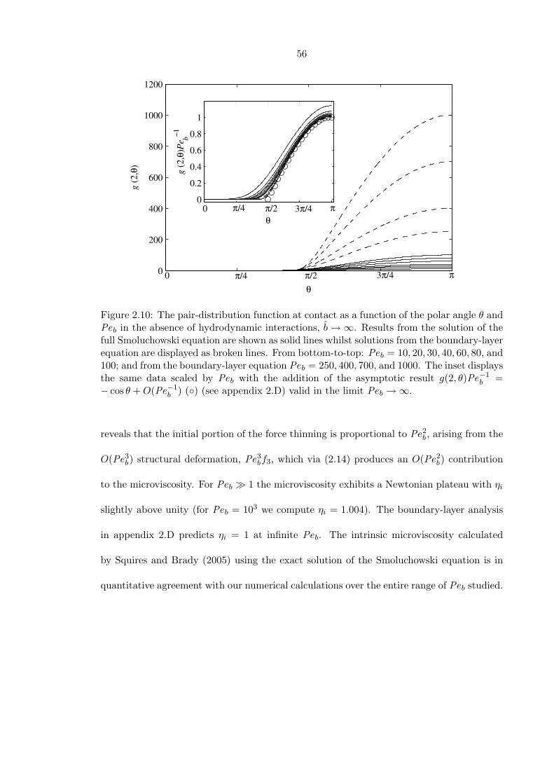
56

0

200

400

600

800

1000

1200

θ

g (2

,θ)

0

0.2

0.4

0.6

0.8

1

θ

g (2

,θ)P

e b−1

π/4 π/2 3π/4 π 0

0 π/4 π/2 3π/4 π

Figure 2.10: The pair-distribution function at contact as a function of the polar angle θ andPeb in the absence of hydrodynamic interactions, b→∞. Results from the solution of thefull Smoluchowski equation are shown as solid lines whilst solutions from the boundary-layerequation are displayed as broken lines. From bottom-to-top: Peb = 10, 20, 30, 40, 60, 80, and100; and from the boundary-layer equation Peb = 250, 400, 700, and 1000. The inset displaysthe same data scaled by Peb with the addition of the asymptotic result g(2, θ)Pe−1

b =− cos θ +O(Pe−1

b ) () (see appendix 2.D) valid in the limit Peb →∞.

reveals that the initial portion of the force thinning is proportional to Pe2b , arising from the

O(Pe3b) structural deformation, Pe3

bf3, which via (2.14) produces an O(Pe2b) contribution

to the microviscosity. For Peb 1 the microviscosity exhibits a Newtonian plateau with ηi

slightly above unity (for Peb = 103 we compute ηi = 1.004). The boundary-layer analysis

in appendix 2.D predicts ηi = 1 at infinite Peb. The intrinsic microviscosity calculated

by Squires and Brady (2005) using the exact solution of the Smoluchowski equation is in

quantitative agreement with our numerical calculations over the entire range of Peb studied.

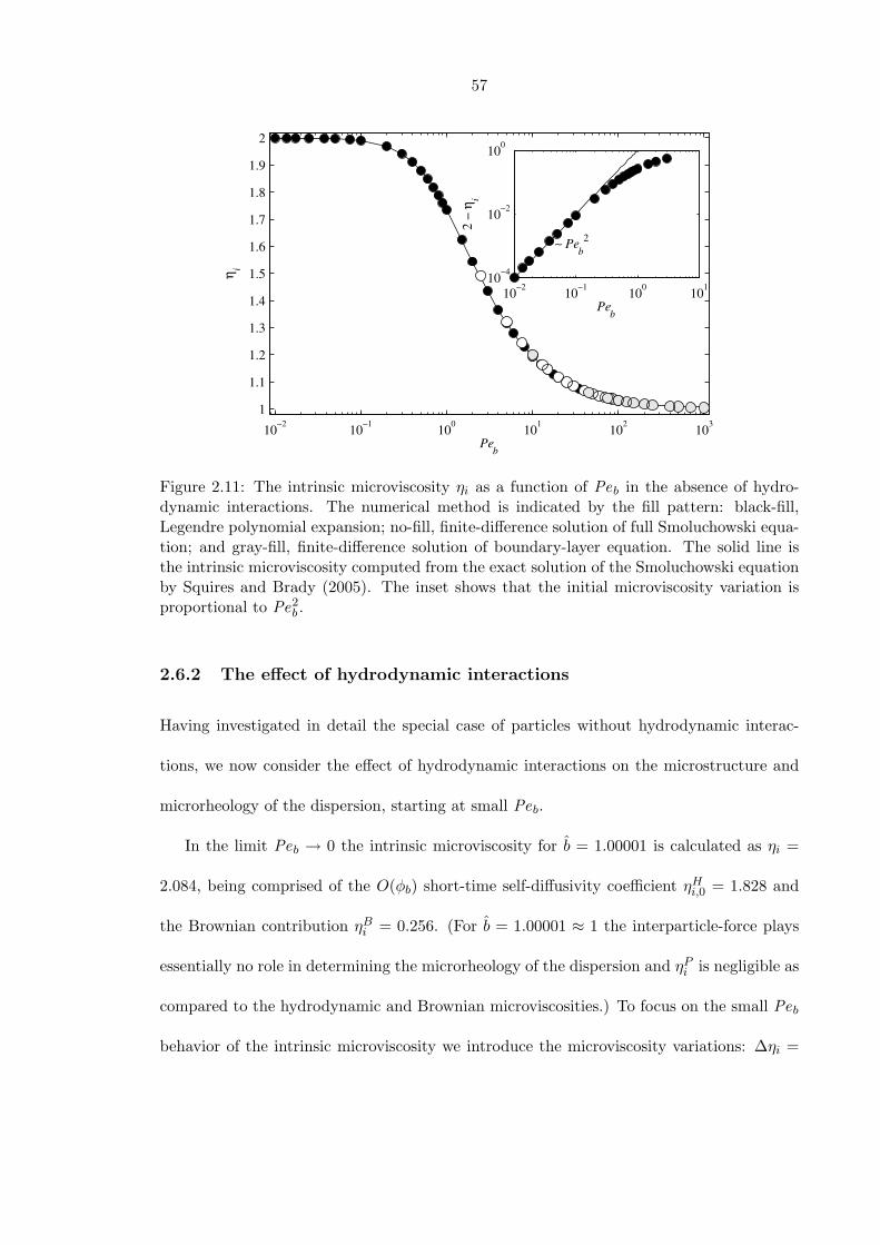
57

10−2 10−1 100 101 102 1031

1.1

1.2

1.3

1.4

1.5

1.6

1.7

1.8

1.9

2

Peb

η i

10−2 10−1 100 10110−4

10−2

100

Peb

2 −

η i

∼ Peb2

Figure 2.11: The intrinsic microviscosity ηi as a function of Peb in the absence of hydro-dynamic interactions. The numerical method is indicated by the fill pattern: black-fill,Legendre polynomial expansion; no-fill, finite-difference solution of full Smoluchowski equa-tion; and gray-fill, finite-difference solution of boundary-layer equation. The solid line isthe intrinsic microviscosity computed from the exact solution of the Smoluchowski equationby Squires and Brady (2005). The inset shows that the initial microviscosity variation isproportional to Pe2

b .

2.6.2 The effect of hydrodynamic interactions

Having investigated in detail the special case of particles without hydrodynamic interac-

tions, we now consider the effect of hydrodynamic interactions on the microstructure and

microrheology of the dispersion, starting at small Peb.

In the limit Peb → 0 the intrinsic microviscosity for b = 1.00001 is calculated as ηi =

2.084, being comprised of the O(φb) short-time self-diffusivity coefficient ηHi,0 = 1.828 and

the Brownian contribution ηBi = 0.256. (For b = 1.00001 ≈ 1 the interparticle-force plays

essentially no role in determining the microrheology of the dispersion and ηPi is negligible as

compared to the hydrodynamic and Brownian microviscosities.) To focus on the small Peb

behavior of the intrinsic microviscosity we introduce the microviscosity variations: ∆ηi =

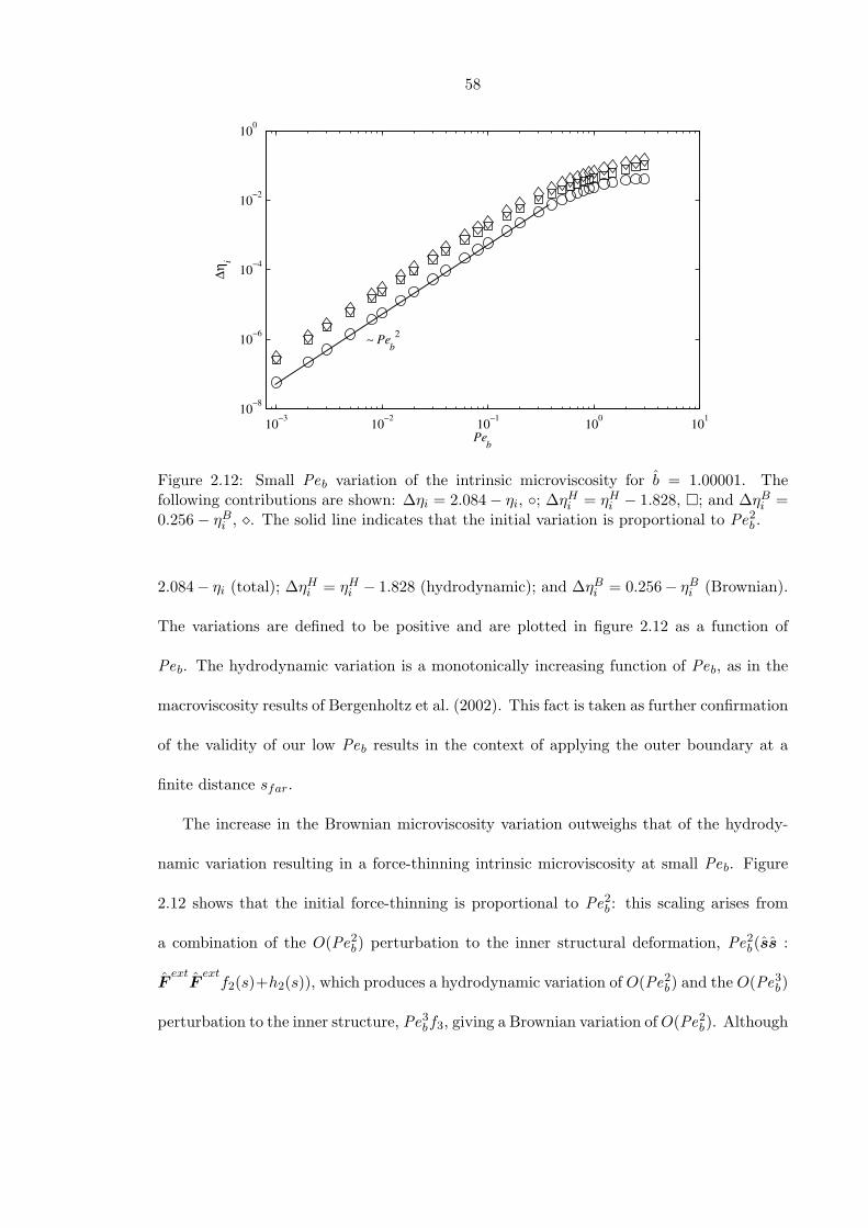
58

10−3 10−2 10−1 100 10110−8

10−6

10−4

10−2

100

Peb

∆ηi

∼ Peb2

Figure 2.12: Small Peb variation of the intrinsic microviscosity for b = 1.00001. Thefollowing contributions are shown: ∆ηi = 2.084− ηi, ; ∆ηH

i = ηHi − 1.828, ; and ∆ηB

i =0.256− ηB

i , . The solid line indicates that the initial variation is proportional to Pe2b .

2.084− ηi (total); ∆ηHi = ηH

i − 1.828 (hydrodynamic); and ∆ηBi = 0.256− ηB

i (Brownian).

The variations are defined to be positive and are plotted in figure 2.12 as a function of

Peb. The hydrodynamic variation is a monotonically increasing function of Peb, as in the

macroviscosity results of Bergenholtz et al. (2002). This fact is taken as further confirmation

of the validity of our low Peb results in the context of applying the outer boundary at a

finite distance sfar.

The increase in the Brownian microviscosity variation outweighs that of the hydrody-

namic variation resulting in a force-thinning intrinsic microviscosity at small Peb. Figure

2.12 shows that the initial force-thinning is proportional to Pe2b : this scaling arises from

a combination of the O(Pe2b) perturbation to the inner structural deformation, Pe2

b(ss :

Fext

Fextf2(s)+h2(s)), which produces a hydrodynamic variation of O(Pe2

b) and the O(Pe3b)

perturbation to the inner structure, Pe3bf3, giving a Brownian variation ofO(Pe2

b). Although

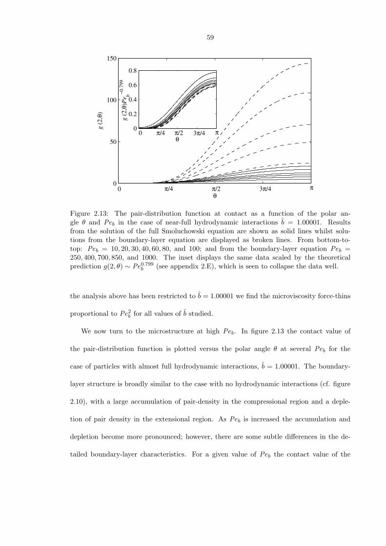
59

0

50

100

150

θ

g (2

,θ)

0

0.2

0.4

0.6

0.8

θ

g (2

,θ)P

e b−0.7

99

π 3π/4 π/2 π/4 0

0 π/4 π/2 3π/4 π

Figure 2.13: The pair-distribution function at contact as a function of the polar an-gle θ and Peb in the case of near-full hydrodynamic interactions b = 1.00001. Resultsfrom the solution of the full Smoluchowski equation are shown as solid lines whilst solu-tions from the boundary-layer equation are displayed as broken lines. From bottom-to-top: Peb = 10, 20, 30, 40, 60, 80, and 100; and from the boundary-layer equation Peb =250, 400, 700, 850, and 1000. The inset displays the same data scaled by the theoreticalprediction g(2, θ) ∼ Pe0.799

b (see appendix 2.E), which is seen to collapse the data well.

the analysis above has been restricted to b = 1.00001 we find the microviscosity force-thins

proportional to Pe2b for all values of b studied.

We now turn to the microstructure at high Peb. In figure 2.13 the contact value of

the pair-distribution function is plotted versus the polar angle θ at several Peb for the

case of particles with almost full hydrodynamic interactions, b = 1.00001. The boundary-

layer structure is broadly similar to the case with no hydrodynamic interactions (cf. figure

2.10), with a large accumulation of pair-density in the compressional region and a deple-

tion of pair density in the extensional region. As Peb is increased the accumulation and

depletion become more pronounced; however, there are some subtle differences in the de-

tailed boundary-layer characteristics. For a given value of Peb the contact value of the

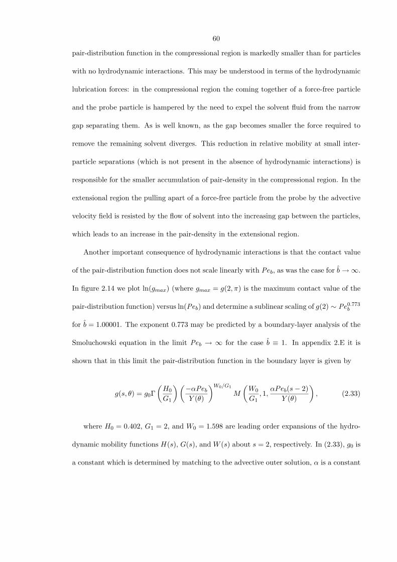
60

pair-distribution function in the compressional region is markedly smaller than for particles

with no hydrodynamic interactions. This may be understood in terms of the hydrodynamic

lubrication forces: in the compressional region the coming together of a force-free particle

and the probe particle is hampered by the need to expel the solvent fluid from the narrow

gap separating them. As is well known, as the gap becomes smaller the force required to

remove the remaining solvent diverges. This reduction in relative mobility at small inter-

particle separations (which is not present in the absence of hydrodynamic interactions) is

responsible for the smaller accumulation of pair-density in the compressional region. In the

extensional region the pulling apart of a force-free particle from the probe by the advective

velocity field is resisted by the flow of solvent into the increasing gap between the particles,

which leads to an increase in the pair-density in the extensional region.

Another important consequence of hydrodynamic interactions is that the contact value

of the pair-distribution function does not scale linearly with Peb, as was the case for b→∞.

In figure 2.14 we plot ln(gmax) (where gmax = g(2, π) is the maximum contact value of the

pair-distribution function) versus ln(Peb) and determine a sublinear scaling of g(2) ∼ Pe0.773b

for b = 1.00001. The exponent 0.773 may be predicted by a boundary-layer analysis of the

Smoluchowski equation in the limit Peb → ∞ for the case b ≡ 1. In appendix 2.E it is

shown that in this limit the pair-distribution function in the boundary layer is given by

g(s, θ) = g0Γ(H0

G1

)(−αPeb

Y (θ)

)W0/G1

M

(W0

G1, 1,

αPeb(s− 2)Y (θ)

), (2.33)

where H0 = 0.402, G1 = 2, and W0 = 1.598 are leading order expansions of the hydro-

dynamic mobility functions H(s), G(s), and W (s) about s = 2, respectively. In (2.33), g0 is

a constant which is determined by matching to the advective outer solution, α is a constant

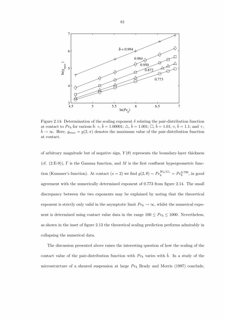
61

4.5 5 5.5 6 6.5 73

4

5

6

7

ln(Peb)

ln(g

max

)

δ = 0.994

0.9840.950

0.872

0.773

Figure 2.14: Determination of the scaling exponent δ relating the pair-distribution functionat contact to Peb for various b: , b = 1.00001; 4, b = 1.001; , b = 1.01; , b = 1.1; and +,b→∞. Here, gmax = g(2, π) denotes the maximum value of the pair-distribution functionat contact.

of arbitrary magnitude but of negative sign, Y (θ) represents the boundary-layer thickness

(cf. (2.E-9)), Γ is the Gamma function, and M is the first confluent hypergeometric func-

tion (Kummer’s function). At contact (s = 2) we find g(2, θ) ∼ PeW0/G1

b = Pe0.799b , in good

agreement with the numerically determined exponent of 0.773 from figure 2.14. The small

discrepancy between the two exponents may be explained by noting that the theoretical

exponent is strictly only valid in the asymptotic limit Peb →∞, whilst the numerical expo-

nent is determined using contact value data in the range 100 ≤ Peb ≤ 1000. Nevertheless,

as shown in the inset of figure 2.13 the theoretical scaling prediction performs admirably in

collapsing the numerical data.

The discussion presented above raises the interesting question of how the scaling of the

contact value of the pair-distribution function with Peb varies with b. In a study of the

microstructure of a sheared suspension at large Peb Brady and Morris (1997) conclude,

62

via an analytical boundary-layer study of the appropriate Smoluchowski equation, that

g(2) ∼ Peb for all b except in the so-called case of ‘pure-hydrodynamics’ b ≡ 1, where

g(2) ∼ Pe0.78b . Stokesian Dynamics simulations of concentrated Brownian suspensions (at

volume fractions of φ = 0.30 and φ = 0.45) in simple-shear flow performed by Morris and

Katyal (1995) indicate that g(2) ∼ Pe0.70b for b = 1.00025 in the range 1 ≤ Peb ≤ 1000, as

opposed to the linear scaling predicted by Brady and Morris (1997). This discrepancy in

the two studies may be attributed to the neglect of the divergence of the relative-velocity

field of two particles by Brady and Morris (1997), which plays a crucial role in setting

the microstructure at small interparticle separations for suspensions possessing very short-

range excluded volume interactions (b − 1 1). Mathematically, the non-zero divergence

of the relative-velocity field states that the phase space of pair-trajectories is not volume

conserving; physically, it acts as a source of pair-density in the compressional regions of

the flow and a sink in the extensional regions. (Note, although the relative-velocity field

of two particles has a non-zero divergence, the Newtonian suspending fluid is, of course,

incompressible.) Let us define the exponent δ = δ(b) such that g(2) ∼ Peδb . In figure 2.14

the exponent δ is determined for several values of b using data from our numerical solution

of the Smoluchowski equation in the range 100 ≤ Peb ≤ 1000. We find that δ changes

continuously between the limits of δ = 0.773 at b = 1.00001 to δ = 1 as b → ∞. Whether

this continuous change may be predicted by an analytical boundary-layer theory of the

Smoluchowski equation for arbitrary b is left as a future study.

In addition to affecting the microstructure of the dispersion hydrodynamic interactions

play a profound role in setting its microrheology. Let us first consider the microrheology of

the suspension for b close to unity, where the thermodynamic radius b is only slightly larger

than the hydrodynamic radius a, so that the particles experience nearly full hydrodynamic

63

0

0.5

1

1.5

2

2.4

0

0.5

1

1.5

2

2.4

10 10 10 10 10 10 10 10 10 10 10−2 −1 0 1 2 3 −1 0 1 2 3

b/a = 1.00001 b/a = 1.001

b/a = 1.01 b/a = 1.1

Peb

η i

Figure 2.15: Contributions to the intrinsic microviscosity ηi as a function of Peb for various b:, total; , hydrodynamic; , Brownian; and 4, interparticle force. The numerical methodis indicated by the fill pattern: black-fill, Legendre polynomial expansion; no-fill, finite-difference solution of full Smoluchowski equation; and gray-fill, finite-difference solution ofthe boundary-layer equation.

interactions. In figure 2.15 we plot the intrinsic microviscosity and its three constituents

as a function of Peb for b = 1.00001, b = 1.001, b = 1.01, and b = 1.1. For b = 1.00001

and b = 1.001 it is observed that the interparticle contribution to the intrinsic microviscos-

ity is essentially negligible as compared to the Brownian and hydrodynamic components.

For small Peb the intrinsic viscosity exhibits a Newtonian plateau which is primarily de-

termined by the hydrodynamic contribution although a smaller, yet significant, Brownian

contribution is present. Of course, the value of the intrinsic microviscosity at this plateau

is nothing but the O(φb) correction to the long-time self-diffusivity, as discussed in § 2.4.2.

On increasing Peb to O(1) the Brownian and hydrodynamic microviscosities decrease and

increase, respectively. The decrease in the Brownian contribution outweighs the increase

in the hydrodynamic contribution (cf. figure 2.12) causing the intrinsic microviscosity to

64

force-thin up to Peb ≈ 3 for b = 1.00001 and Peb ≈ 3.5 for b = 1.001, at which point it

attains a minimum. Beyond this minimum the Brownian contribution becomes negligible

and the hydrodynamic contribution increases steadily, which has the net effect of making

the intrinsic microviscosity force-thicken. As Peb is increased the advective flux (set up

through the relative velocity field induced by the external force on the probe) of force-

free particles towards the probe particle becomes stronger. For large Peb this advective

flux ‘squeezes’ particles into close-contact with the probe, where they experience highly

resistive lubrication forces, which is, in part, the cause of continuous force-thickening for

Peb ∼ O(1) and beyond. However, this is not the whole story: the moving probe not only

‘pushes’ background particles (leading to a high probability-density in the boundary layer

at the front of the probe), but also ‘drags’ background particles that are immediately behind

it, as these particles are ‘stuck’ to the probe due to the lubrication forces (cf. the higher

probability-density downstream of the probe with hydrodynamics (figure 2.13) as compared

to without hydrodynamics (figure 2.10)). Indeed, this ‘dragging’ effect contributes signifi-

cantly to the microviscosity at large Peb. In table 2.1 we split the intrinsic microviscosity at

Peb = 1000 into equilibrium ηHi,0; compressional (or pushing) ηi,c; and extensional (or drag-

ging) ηi,e contributions for full hydrodynamics (b = 1.00001 ≈ 1) and no hydrodynamics

(b→∞). For full hydrodynamics ηi,e/(ηi,e + ηi,c) = 0.351, whilst without hydrodynamics,

for which there is no dragging effect (as the particles do not experience lubrication forces),

ηi,e/(ηi,e + ηi,c) = 0.001. The qualitative picture of the microviscosity as a function of Peb

agrees with that of Bergenholtz et al. (2002) and the Stokesian Dynamics simulations of

concentrated sheared suspensions of Foss and Brady (2000) for the macroviscosity.

On increasing b the qualitative description presented above changes; for b = 1.1 (again,

see figure 2.15) the intrinsic microviscosity has significant contributions from all three of

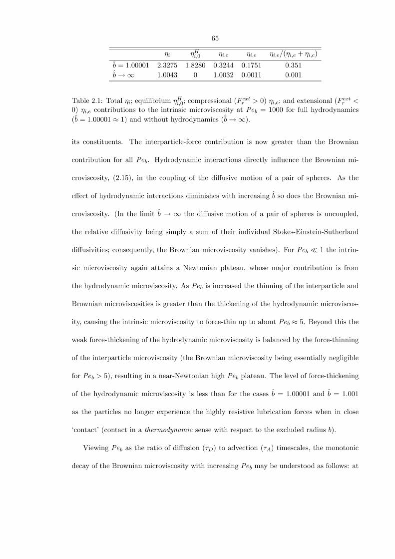
65

ηi ηHi,0 ηi,c ηi,e ηi,e/(ηi,e + ηi,c)

b = 1.00001 2.3275 1.8280 0.3244 0.1751 0.351b→∞ 1.0043 0 1.0032 0.0011 0.001

Table 2.1: Total ηi; equilibrium ηHi,0; compressional (F ext

r > 0) ηi,c; and extensional (F extr <

0) ηi,e contributions to the intrinsic microviscosity at Peb = 1000 for full hydrodynamics(b = 1.00001 ≈ 1) and without hydrodynamics (b→∞).

its constituents. The interparticle-force contribution is now greater than the Brownian

contribution for all Peb. Hydrodynamic interactions directly influence the Brownian mi-

croviscosity, (2.15), in the coupling of the diffusive motion of a pair of spheres. As the

effect of hydrodynamic interactions diminishes with increasing b so does the Brownian mi-

croviscosity. (In the limit b → ∞ the diffusive motion of a pair of spheres is uncoupled,

the relative diffusivity being simply a sum of their individual Stokes-Einstein-Sutherland

diffusivities; consequently, the Brownian microviscosity vanishes). For Peb 1 the intrin-

sic microviscosity again attains a Newtonian plateau, whose major contribution is from

the hydrodynamic microviscosity. As Peb is increased the thinning of the interparticle and

Brownian microviscosities is greater than the thickening of the hydrodynamic microviscos-

ity, causing the intrinsic microviscosity to force-thin up to about Peb ≈ 5. Beyond this the

weak force-thickening of the hydrodynamic microviscosity is balanced by the force-thinning

of the interparticle microviscosity (the Brownian microviscosity being essentially negligible

for Peb > 5), resulting in a near-Newtonian high Peb plateau. The level of force-thickening

of the hydrodynamic microviscosity is less than for the cases b = 1.00001 and b = 1.001

as the particles no longer experience the highly resistive lubrication forces when in close

‘contact’ (contact in a thermodynamic sense with respect to the excluded radius b).

Viewing Peb as the ratio of diffusion (τD) to advection (τA) timescales, the monotonic

decay of the Brownian microviscosity with increasing Peb may be understood as follows: at

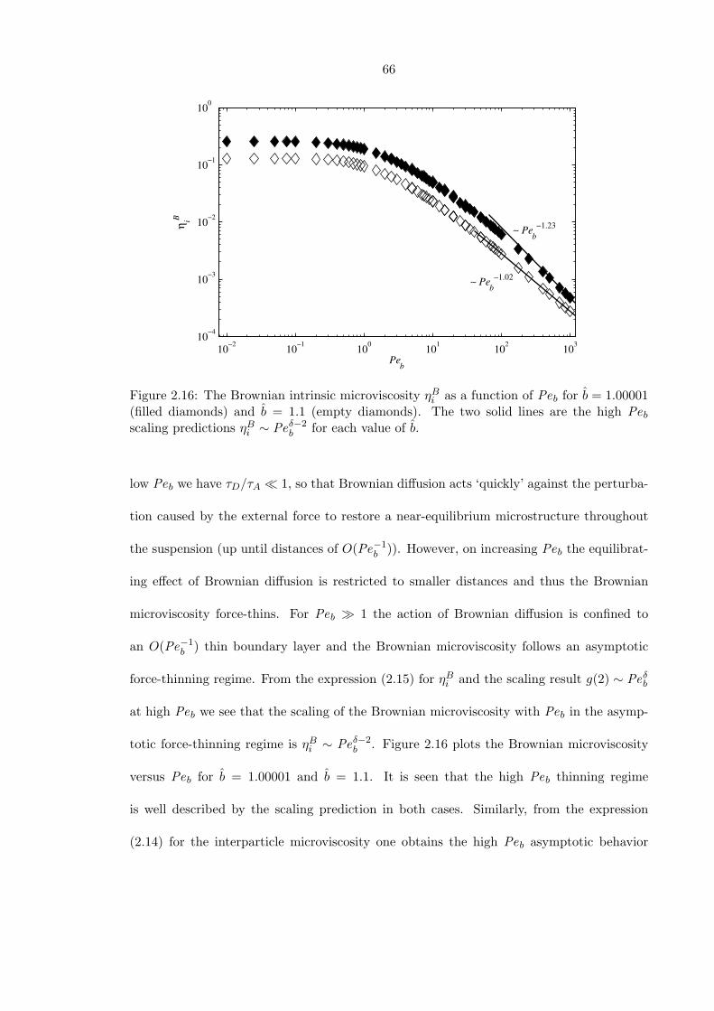
66

10−2 10−1 100 101 102 10310−4

10−3

10−2

10−1

100

Peb

η iB

∼ Peb−1.02

∼ Peb−1.23

Figure 2.16: The Brownian intrinsic microviscosity ηBi as a function of Peb for b = 1.00001

(filled diamonds) and b = 1.1 (empty diamonds). The two solid lines are the high Peb

scaling predictions ηBi ∼ Peδ−2

b for each value of b.

low Peb we have τD/τA 1, so that Brownian diffusion acts ‘quickly’ against the perturba-

tion caused by the external force to restore a near-equilibrium microstructure throughout

the suspension (up until distances of O(Pe−1b )). However, on increasing Peb the equilibrat-

ing effect of Brownian diffusion is restricted to smaller distances and thus the Brownian

microviscosity force-thins. For Peb 1 the action of Brownian diffusion is confined to

an O(Pe−1b ) thin boundary layer and the Brownian microviscosity follows an asymptotic

force-thinning regime. From the expression (2.15) for ηBi and the scaling result g(2) ∼ Peδ

b

at high Peb we see that the scaling of the Brownian microviscosity with Peb in the asymp-

totic force-thinning regime is ηBi ∼ Peδ−2

b . Figure 2.16 plots the Brownian microviscosity

versus Peb for b = 1.00001 and b = 1.1. It is seen that the high Peb thinning regime

is well described by the scaling prediction in both cases. Similarly, from the expression

(2.14) for the interparticle microviscosity one obtains the high Peb asymptotic behavior

67

ηPi ∼ G(2b)Peδ−1

b . This implies that for all finite b (for which δ < 1) the interparticle

microviscosity should be a weakly decaying function Peb at large Peb. Only in the absence

of hydrodynamic interactions (b → ∞, where δ = 1) does the interparticle microviscosity

attain a true high Peb Newtonian plateau.

Unlike the Brownian and interparticle microviscosities, which for Peb 1 are deter-

mined primarily by the boundary-layer structure, the hydrodynamic microviscosity has

contributions arising throughout the entire domain s ≥ 2. The boundary layer has a char-

acteristic size of O(Pe−1b ) and contains an O(Peδ

b) buildup of pair-density, which from (2.12)

implies an O(Peδ−1b ) contribution to ηH

i . The O(1) pair-density in the advective ‘outer’ re-

gion (s− 2 O(Pe−1b )) yields an O(1) (i.e. independent of Peb) contribution to ηH

i . Thus,

in the limit Peb → ∞ the hydrodynamic microviscosity takes the form ηHi ∼ α + βPeδ−1

b ,

where α and β are functions of b only. This asymptotic form may be used to extrapolate

the large Peb results for ηHi to the Peb →∞ limit. The coefficients α and β are determined

from a nonlinear regression analysis of ηHi versus Peb plots, using ηH

i data for Peb ≥ 200.

Figure 2.17 displays an extrapolation of the intrinsic microviscosity ηi for b = 1.00001, for

which ηHi ∼ 2.511− 0.879Pe−0.227

b (recall that for b = 1.00001 at large Peb both ηBi and ηP

i

are negligible as compared to ηHi ). At infinite Peb the extrapolation predicts ηi = 2.511,

in good agreement with the studies of Batchelor and Wen (1982) and Almog and Brenner

(1997) who both find that ηi = 2.52 for b ≡ 1 in the ‘Falling-Ball’ limit Pe−1b ≡ 0. Fur-

thermore, for b ≡ 1 and Pe−1b ≡ 0 the pair-distribution function is spherically symmetric

(cf. (2.E-1)), i.e. for a given radial separation there is an equal probability of finding a

background particle in the compressional or extensional regions around the probe. Hence,

ηi must have equal compressional/pushing (ηi,c) and extensional/dragging (ηi,e) contribu-

tions. As the equilibrium contribution ηHi,0 = 1.83 for b ≡ 1 this gives ηi,c = ηi,e = 0.35 at

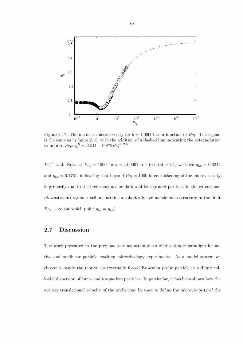
68

10−2 100 102 104 106 108 10102

2.1

2.2

2.3

2.4

2.5 2.52

Peb

η i

Figure 2.17: The intrinsic microviscosity for b = 1.00001 as a function of Peb. The legendis the same as in figure 2.15, with the addition of a dashed line indicating the extrapolationto infinite Peb: ηH

i ∼ 2.511− 0.879Pe−0.227b .

Pe−1b ≡ 0. Now, at Peb = 1000 for b = 1.00001 ≈ 1 (see table 2.1) we have ηi,c = 0.3244

and ηi,e = 0.1751, indicating that beyond Peb = 1000 force-thickening of the microviscosity

is primarily due to the increasing accumulation of background particles in the extensional

(downstream) region, until one attains a spherically symmetric microstructure in the limit

Peb →∞ (at which point ηi,c = ηi,e).

2.7 Discussion

The work presented in the previous sections attempts to offer a simple paradigm for ac-

tive and nonlinear particle tracking microrheology experiments. As a model system we

choose to study the motion an externally forced Brownian probe particle in a dilute col-

loidal dispersion of force- and torque-free particles. In particular, it has been shown how the

average translational velocity of the probe may be used to define the microviscosity of the

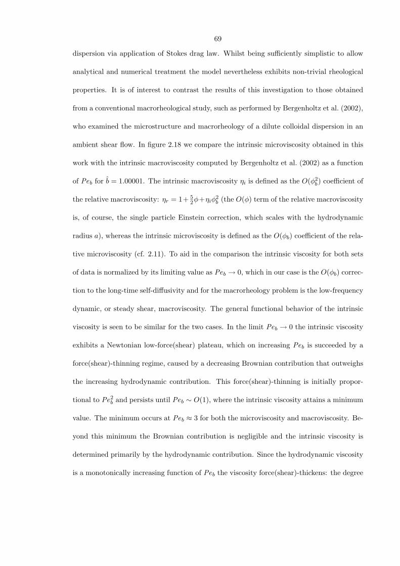
69

dispersion via application of Stokes drag law. Whilst being sufficiently simplistic to allow

analytical and numerical treatment the model nevertheless exhibits non-trivial rheological

properties. It is of interest to contrast the results of this investigation to those obtained

from a conventional macrorheological study, such as performed by Bergenholtz et al. (2002),

who examined the microstructure and macrorheology of a dilute colloidal dispersion in an

ambient shear flow. In figure 2.18 we compare the intrinsic microviscosity obtained in this

work with the intrinsic macroviscosity computed by Bergenholtz et al. (2002) as a function

of Peb for b = 1.00001. The intrinsic macroviscosity ηi is defined as the O(φ2b) coefficient of

the relative macroviscosity: ηr = 1+ 52φ+ηiφ

2b (the O(φ) term of the relative macroviscosity

is, of course, the single particle Einstein correction, which scales with the hydrodynamic

radius a), whereas the intrinsic microviscosity is defined as the O(φb) coefficient of the rela-

tive microviscosity (cf. 2.11). To aid in the comparison the intrinsic viscosity for both sets

of data is normalized by its limiting value as Peb → 0, which in our case is the O(φb) correc-

tion to the long-time self-diffusivity and for the macrorheology problem is the low-frequency

dynamic, or steady shear, macroviscosity. The general functional behavior of the intrinsic

viscosity is seen to be similar for the two cases. In the limit Peb → 0 the intrinsic viscosity

exhibits a Newtonian low-force(shear) plateau, which on increasing Peb is succeeded by a

force(shear)-thinning regime, caused by a decreasing Brownian contribution that outweighs

the increasing hydrodynamic contribution. This force(shear)-thinning is initially propor-

tional to Pe2b and persists until Peb ∼ O(1), where the intrinsic viscosity attains a minimum

value. The minimum occurs at Peb ≈ 3 for both the microviscosity and macroviscosity. Be-

yond this minimum the Brownian contribution is negligible and the intrinsic viscosity is

determined primarily by the hydrodynamic contribution. Since the hydrodynamic viscosity

is a monotonically increasing function of Peb the viscosity force(shear)-thickens: the degree

70

10−2 10−1 100 101 1020.9

0.95

1

1.05

1.1

1.15

Peb

η i(Pe b) /

ηi(P

e b → 0

)

10−2 100 1020.4

0.6

0.8

1

Pebη i(P

e b) / η

i(Pe b →

0)

Figure 2.18: Comparison of the intrinsic microviscosity as a function of Peb for b = 1.00001obtained in this investigation () with the intrinsic macroviscosity results of Bergenholtzet al. (2002) (). The filling pattern indicates the method of numerical solution as infigure 2.11. The inset shows a comparison of the intrinsic viscosities in the absence ofhydrodynamic interactions b→∞. For the microviscosity the Peclet number is defined asPeb = F0/(2kT/b), whilst for the macroviscosity Peb = 6πηabγ/(2kT/b), where γ is theshear-rate of the imposed shear flow.

of thickening is significantly greater for the microviscosity (ηi/ηi,0 ≈ 1.10 at Peb = 500)

as compared to the macroviscosity (ηi/ηi,0 ≈ 1.02 at Peb = 500). Our results support the

claim of Bergenholtz et al. (2002) that shear-thickening of the macroviscosity of colloidal

dispersions at high Peb is a two-body (or dilute) effect, which arises as a consequence of

the boundary-layer formation at small interparticle separations.

When the particles do not experience hydrodynamic interactions (b→∞) the intrinsic

microviscosity and intrinsic macroviscosity are determined exclusively from the interparticle-

force contribution. It was found that the microviscosity thins monotonically with increasing

Peb from a Newtonian plateau in the limit Peb → 0 to a second Newtonian plateau at infinite

Peb. Qualitatively similar behavior is seen for the intrinsic macroviscosity, as shown by the

71

inset of figure 2.18.

The comparison of micro- and macro-viscosity raises several issues that warrant further

elaboration. As noted above, the micro- and macro-viscosity scale differently with the back-

ground particle volume fraction φb: the microstructurally-dependent contribution (which

has hitherto been termed the intrinsic viscosity) to the microviscosity is O(φb), whilst for

the macroviscosity it is O(φ2b). Knowing these scalings in advance allows one to compare

the micro- and macro-viscosity in a consistent manner. However, for more complicated (or

unknown) materials such scalings may not be known a priori, and the comparison between

micro and macro may not be so agreeable. Nonetheless, as mentioned in § 2.1, dispari-

ties between micro- and macro-rheological measurements are denotive of the fundamental

physical differences in the two techniques. Therefore, such discrepancies do not render the

microrheological data invalid; on the contrary, one should strive to understand the addi-

tional information contained in them, and, to this end, it is essential to develop detailed

theoretical models for active microrheology experiments.

The comparison in figure 2.18 is between the microviscosity at fixed force and the macro-

viscosity at fixed shear rate. Properly, one should compared the fixed force microviscosity

to the fixed stress macroviscosity (and, likewise, fixed velocity micro to fixed shear rate

macro). However, in the dilute limit it is easy to show that the fixed stress and fixed

shear rate macroviscosities are identical. Thus, the comparison in figure 2.18 is legitimate.

In contrast, as demonstrated by Squires and Brady (2005) and discussed below, the fixed

force and fixed velocity microviscosities are different in the dilute limit. Furthermore, in

the fixed velocity mode the probe does not move diffusively, and the relative diffusivity is

the background particle (Stokes-Einstein-Sutherland) diffusivity D. In fixed force mode the

probe moves deterministically and diffusively; thus, the relative diffusivity is 2D. Therefore,

72

the Peclet number for fixed velocity (F0/(kT/b)) is twice that for fixed force (F0/(2kT/b)).

Lastly, although one can compare the micro- and macro-viscosity, microrheology can only

determine a scalar viscosity (at least for a single spherical probe: a non-spherical probe or

two spherical probes may yield more information), whereas in macrorheology the full stress

tensor is obtainable, including normal stress differences and an isotropic osmotic pressure

(Bergenholtz et al. 2002).

In this study it was assumed (for simplicity) that the probe particle is of the same size

as the background particles; in practice, this is not always the case. For instance, Habdas

et al. (2004) in their investigation of the forced motion of a magnetic bead in a dense

colloidal dispersion used bead particles of roughly twice the size of the dispersion particles.

A natural question to pose is: how does the calculated microviscosity of the dispersion vary

with the size of the probe particle? Almog and Brenner (1997) have addressed this question

in the so-called ‘Falling-Ball’ limit, Pe−1 ≡ 0, for b ≡ 1. They find that when the probe

sphere is much larger than the suspended spheres one recovers Einstein’s viscosity correction

ηi = 2.5. On the other hand, when the probe is much smaller than the suspended spheres

they observe ηi → ∞. In the absence of hydrodynamic interactions (b → ∞) Squires and

Brady (2005) have solved the pair problem for all Peb and all size ratios. They show that

ηi ∼ (1 + λ)2/2, where λ is the size ratio of probe particle to background particle. It would

be of interest to examine how the microviscosity varies with the size of the probe particle

at finite Peb and whether or not the scaling results of Squires and Brady (2005) hold as

hydrodynamic interactions are brought in.

An alternative to fixing the force on the probe is to fix its velocity. In this case the

ensemble averaged force on the probe may now be related to the suspension’s microviscosity

via the Stokes drag formula. A natural question arises as to whether the fixed force and fixed

73

velocity procedures give the same intrinsic microviscosity. Almog and Brenner (1997) have

shown in the ‘Falling-Ball’ limit (Peb → ∞) that the intrinsic microviscosity does differ

when calculated using fixed-force or fixed-velocity probe particles. In fact, the intrinsic

viscosity measured using the fixed-velocity probe is always greater than that obtained for

the fixed-force probe, except in the limit where the probe particle is much larger than the

suspended spheres for which one recovers Einstein’s viscosity correction in both cases. In

the absence of hydrodynamic interactions and for all Peb, Squires and Brady (2005) find

that the ratio of fixed-velocity to fixed-force intrinsic microviscosities is (1 + λ)/λ. Once

again, the fixed-velocity microviscosity is always greater than the fixed-force microviscosity

except in the limit where the probe is much larger than the background particles, where they

are equal. Physically speaking, the fixed-velocity probe expends more energy in pushing

surrounding particles out of its path than the fixed-force probe which may pass around

any obstructing particles. Almog and Brenner (1997) state the discrepancy between the

fixed-force and fixed-velocity microviscosities to be indicative of the fundamentally non-

continuum nature of the suspension. Whether this discrepancy persists for finite Peb is not

known (except in the special case b→∞, Squires and Brady 2005) and is clearly a question

of interest as it suggests the intriguing possibility of applying microrheological techniques

to study the non-continuum nature of soft heterogeneous materials.

In conclusion, one may view this investigation as a step towards laying a theoretical

foundation for active and nonlinear microrheology. Adopting the forced motion of a single

probe particle in an otherwise quiescent colloidal dispersion as a simple paradigm for active

tracking experiments, we have shown that, when appropriately scaled, the microviscosity

of the dispersion is in qualitative agreement with the macroviscosity. However, for more

complex materials, where the relevant micro and macro scalings are not known a priori,

74

micro- and macro-rheological data may not be in such good agreement, and great care is to

be taken in the interpretation of the microrheology experiments. Nevertheless, our study

suggests that active microrheology has the potential to be a valuable tool with which to

explore the rich nonlinear rheology of complex fluids.

75

2.8 Bibliography

M. Abramowitz and I. Stegun. Handbook of mathematical functions. Dover, 1972.

A. Acrvios and T. D. Taylor. Heat and mass transfer from single spheres in Stokes flow.

Phys. Fluids, 5:387–394, 1965.

Y. Almog and H. Brenner. Non-continuum anomalies in the apparent viscosity experienced

by a test sphere moving through an otherwise quiescent suspension. Phys. Fluids, 9:

16–22, 1997.

H. A. Barnes, J. F. Hutton, and K. Walters. An Introduction to Rheology. Elsevier, 1989.

G. K. Batchelor. Brownian diffusion of particles with hydrodynamic interaction. J. Fluid

Mech., 74:1–29, 1976.

G. K. Batchelor. Sedimentation in a dilute polydisperse system of interacting spheres. Part

1. General theory. J. Fluid Mech., 119:379–408, 1982.

G. K. Batchelor. Diffusion in a dilute polydisperse system of interacting spheres. J. Fluid

Mech., 131:155–176, 1983.

G. K. Batchelor and C. S. Wen. Sedimentation in a dilute polydisperse system of interacting

spheres. Part 2. Numerical results. J. Fluid Mech., 124:495–528, 1982.

J. Bergenholtz, J. F. Brady, and M. Vicic. The non-Newtonian rheology of dilute colloidal

suspensions. J. Fluid Mech., 456:239–275, 2002.

J. F. Brady. The long-time self-diffusivity in concentrated colloidal dispersions. J. Fluid

Mech., 272:109–133, 1994.

76

J. F. Brady and J. F. Morris. Microstructure of strongly sheared suspensions and its impact

on rheology and diffusion. J. Fluid Mech., 348:103–139, 1997.

J. C. Crocker, M. T. Valentine, E. R. Weeks, T. Gisler, P. D. Kaplan, A. G. Yodh, and

D. A. Weitz. Two-point microrheology of inhomogeneous soft materials. Phys. Rev. Lett.,

84:888–891, 2000.

R. H. Davis and N. A. Hill. Hydrodynamic diffusion of a sphere sedimenting through a

dilute suspension of neutrally buoyant spheres. J. Fluid Mech., 236:513–533, 1992.

D. R. Foss and J. F. Brady. Structure, diffusion and rheology of Brownian suspensions by

Stokesian Dynamics simulation. J. Fluid Mech., 407:167–200, 2000.

F. Gittes, B. Schnurr, P. D. Olmsted, F. C. MacKintosh, and C. F. Schimdt. Microscopic

viscoelasticity: shear moduli of soft materials determined from thermal fluctuations. Phys.

Rev. Lett., 79:3286–3289, 1997.

P. Habdas, D. Schaar, A. C. Levitt, and E. R. Weeks. Forced motion of a probe particle

near the colloidal glass transition. Europhys. Lett., 79:477–483, 2004.

D. J. Jeffrey and Y. Onishi. Calculation of the resistance and mobility functions of two

unequal rigid spheres in low-Reynolds-number flow. J. Fluid Mech., 139:261–290, 1984.

S. Kim and S. J. Karilla. Microhydrodynamics: Principles and Selected Applications.

Butterworth-Heinemann, 1991.

R. A. Lionberger. Shear thinning of coloidal dispersions. J. Rheol., 42:843–863, 1998.

F. C. MacKintosh and C. F. Schmidt. Microrheology. Curr. Opin. Colloid Interface Sci.,

4:300–307, 1999.

77

T. G. Mason, K. Ganesan, J. H. van Zanten, D. Wirtz, and S. C. Kuo. Particle tracking

microrheology of complex fluids. Phys. Rev. Lett., 79:3282–3285, 1997.

T. G. Mason and D. A. Weitz. Optical measurements of frequency-dependent linear vis-

coelastic moduli of complex fluids. Phys. Rev. Lett., 74:1250–1253, 1995.

J. F Morris and B. Katyal. Microstructure from simulated Brownian suspension flows at

large shear rate. Phys. Fluids, 14:1920–1937, 1995.

K. C. Ng. Hypernetted chain solution for the classical one component plasma up to γ = 7000.

J. Chem. Phys, 61:2680–2689, 1974.

W. H. Press, S. A. Teukolsky, W. Vetterling, and B. P. Flannery. Numerical recipes in

FORTRAN. Cambridge University Press, 1992.

J. M. Rallison and E. J. Hinch. The effect of particle interactions on dynamic light scattering

from a dilute suspension. J. Fluid Mech., 167:131–168, 1986.

W. B. Russel, D. A. Saville, and W. R. Schowalter. Colloidal Dispersions. Cambridge

University Press, 1989.

T. M. Squires and J. F. Brady. A simple paradigm for active and nonlinear microrheology.

Phys. Fluids, 17:073101, 2005.

M. Van Dyke. Perturbation Methods in Fluid Mechanics. Parabolic Press, 1975.

T. A. Waigh. Microrheology of complex fluids. Rep. Prog. Phys., 68:685–742, 2005.

78

Appendices to chapter 2

79

2.A The Brownian velocity contribution

In this appendix the result (2.9) for the Brownian velocity contribution is derived. We

consider a collection of colloidal particles subjected to a stochastic Brownian force F B. In

what follows there is an implicit summation over all particles in the suspension.

The Brownian force is characterized by the usual statistical properties

F B(t′) = 0, and F B(t′)F B(t′′) = Fδ(t′ − t

′′), (2.A-1)

where the overline denotes an average over the many collisions of the solvent molecules

with the suspended particles. The appropriate timescale for this average is ts = ms/6πηas

(where ms and as are the mass and radius of a solvent molecule respectively), i.e. the

vorticity diffusion, or inertial relaxation, time of a solvent molecule. The amplitude of

correlation of the Brownian force at times t′and t

′′is given by the fluctuation-dissipation

theorem as F = 2kTRFU , with RFU the multiparticle resistance tensor relating the forces

on the particles to their velocities. This resistance tensor is a function of the instantaneous

configuration, say X(t), of all the particles.

From low Reynolds number fluid dynamics the instantaneous velocity of the particles

due to the Brownian force is UB = MUF ·F B, where MUF = (RFU )−1 is the multiparticle

mobility tensor that relates the velocities of the particles to the forces acting on them. We

need to average this velocity over a time step ∆t, which is long compared to the inertial

relaxation time of a particle, tI = m/6πηa, but much smaller than the diffusive timescale,

80

tD = a2/D, characterizing changes in the configuration of the particles. Doing so we find

1∆t

∫ t+∆t

tUB

i dt′

=1

∆t

∫ t+∆t

tMUF

ij (t′)Fj(t

′)dt

′

= MUFij (t)

1∆t

∫ t+∆t

tFj(t

′)dt

′+∂MUF

ij (t)∂xk

1∆t

∫ t+∆t

t∆Xk(t

′)Fj(t

′)dt

′,

(2.A-2)

where the summation convention is applied to repeated indices, and the configuration

displacement is to leading order ∆Xk(t′) = MUF

kl (t)∫ t

′

0 Fl(t′′)dt

′′. Averaging (2.A-2) over

many solvent collisions and using (2.A-1) we obtain

UB = kT∇ ·MUF ,

where the divergence is taken with respect to the last index of the mobility tensor.

The velocity of an individual particle α is given by UBα = kT

∑Nβ=1 ∇β · MUF

αβ , where

the index β runs over all N particles. In the case of just two particles (say 1 and 2) we

have UB1 = kT (∇1 · MUF

11 + ∇2 · MUF12 ). Employing a center-of-mass coordinate system

(∇r = ∇2 = −∇1) the result (2.9) is recovered.

2.B Finite difference method

In this appendix we describe in detail the finite difference solution of the Smoluchowski

equation that was outlined in § 2.5.2. The finite difference solution is used for Peb ≥ 2, for

which one expects a boundary layer adjacent to the probe in the compressional region of the

relative-velocity field in which there are large gradients in the pair-distribution function. To

accurately capture the behavior of the pair-distribution function in the boundary layer we

81

stretch the radial coordinate via the transformation y = Peb(s−2). Thus, the Smoluchowski

equation (2.29) becomes (with Fext

= −z)

G cos θ∂f

∂y−

Pe−1b H sin θ

2x∂f

∂θ+W cos θ(1 + f)

= G∂2f

∂y2+ Pe−1

b

(dG

ds+G

x

)∂f

∂y+

Pe−2b H

4x2 sin θ∂

∂θ

(sin θ

∂f

∂θ

),

where x = 1+Pe−1b y/2. Whilst paying careful attention to the boundary-layer structure

it is also important to correctly describe the far-field behavior of f(s). To this end, we

perform a second radial coordinate transformation to go from the semi-infinite domain

y ∈ [0,∞) to the finite domain t ∈ [0, 1] via the mapping

t = exp(−ω +

1− ω

1 + y

y

),

where ω is an adjustable parameter. The Smoluchowski equation now reads

G cos θdt

dy

∂f

∂t−

Pe−1b H sin θ

2x∂f

∂θ+W cos θ(1 + f)

= G

(dt

dy

)2 ∂2f

∂t2+(Gd2t

dy2Pe−1

b

dG

ds+G

x

dt

dy

)∂f

∂t

+Pe−2

b H

4x2 sin θ∂

∂θ

(sin θ

∂f

∂θ

),

with the boundary conditions

(dt

dy

)∂f

∂t= cos θ(1 + f) at t = 1,

f = 0 at t = 0.

The Smoluchowski equation is discretized by approximating the radial and angular

82

derivatives by central differences

∂f

∂t=

fj+1,k − fj−1,k

2∆t,

∂2f

∂t2=fj+1,k − 2fj,k + fj−1,k

∆t2,

∂f

∂θ=

fj,k+1 − fj,k−1

2∆θ,

∂2f

∂θ2=fj,k+1 − 2fj,k + fj,k−1

∆θ2,

where j = 1, 2, ..., J and k = 0, 1, ...,K. The interior domain of solution is 0 < t < 1 with

t = j/(J+1) (the points t = 0 and t = 1 are excluded as the radial boundary conditions must

be applied there) and 0 ≤ θ ≤ π with θ = kπ/K. Thus, the node spacings are ∆θ = π/K

and ∆t = 1/(J + 1). Note, though the node spacing is constant in t-space it is not so in

s-space, and via the adjustment of ω one can place a large number of nodes near s = 2

to accurately model the boundary layer. One can make a vector comprising the unknown

structural deformation at each grid point, fj,k, by defining an index i = j + kJ running

from 1 to J(K + 1). This enables the discretized Smoluchowski equation to be written as

the matrix equation A · f = w, with f the unknown structural deformation vector. The

coefficient matrix A is tridiagonal with two fringes, so we may write T ·f = w−(F1+F2)·f ,

where T is the tridiagonal part of A, and F1 and F2 are the fringes. (Here, the term fringe

is used to denote a matrix whose tridiagonal elements are zero.) The matrix equation is

solved by constructing the Jacobi iteration

f (n+1) = T−1 ·(w − (F1 + F2) · f (n)

),

where n is the iteration number. For a particular value of Peb (Peb,2 say) the iteration

input f(0)

Peb,2is the converged result fPeb,1

for the structural deformation at Peb,1 < Peb,2,

i.e. a parameter continuation in Peb is performed. The iteration is deemed to have converged

if the norm ‖f (n+1) − f (n)‖ < ε, where the tolerance ε is typically 10−14. Alternatively, the

83

matrix equation may be written in component form as

aifi−1 + bifi + cifi+1 + difi−J + eifi+J = wi,

where the vectors constituting the tridiagonal matrix T are

ai = G

(dt

dy

)2

∆t−2 − 12

(Gd2t

dy2Pe−1

b

dG

ds+G

x

dt

dy

)∆t−1 +

G

2cos θ

(dt

dy

)∆t−1,

bi = −2G(dt

dy

)2

∆t−2 −Pe−2

b H

2x2∆θ−2 − Pe−1

b W cos θ,

ci = G

(dt

dy

)2

∆t−2 +12

(Gd2t

dy2Pe−1

b

dG

ds+G

x

dt

dy

)∆t−1 − G

2cos θ

(dt

dy

)∆t−1,

the fringe vectors are

di = −Pe−1

b H sin θ4x

∆θ−1 +Pe−2

b H

4x2∆θ−2 −

Pe−2b H

8x2cot θ∆θ−1,

ei =Pe−1

b H sin θ4x

∆θ−1 +Pe−2

b H

4x2∆θ−2 +

Pe−2b H

8x2cot θ∆θ−1,

and the forcing vector is simply wi = Pe−1b W cos θ. It appears from the above that di

and ei are infinite at θ = 0 and θ = π; however, this is just a coordinate singularity and

can easily be eliminated by imposing a natural symmetry boundary condition ∂f/∂θ = 0

(in finite difference terms fj,k+1 = fj,k−1) at θ = 0 and θ = π.

2.C Boundary-layer equation

Our point of departure is the Smoluchowski equation in spherical polar coordinates (2.29).

To focus on the details of the boundary layer in the high Peb limit we introduce the stretched

84

radial coordinate y = Peb(s− 2), yielding the following equation

G∂2f

∂y2+Q

∂f

∂y+

Pe−2b H

4 sin θ∂

∂θ

(sin θ

∂f

∂θ

)= −Pe−1

b

(H

2F ext

θ

∂f

∂θ+WF ext

r (1 + f)), (2.C-1)

where terms of O(Pe−3b ) and higher have been neglected. The smallest term discarded

is O(y2Pe−3b ) which indicates that (2.C-1) is not uniformly valid. However, the loss of

uniformity occurs at y ∼ O(Pe1/2b ) and hence should not affect the boundary-layer structure

(for which y ∼ O(1)) of the pair-distribution function at large Peb. The function Q is given

by

Q = F extr G+

dG

dy+ Pe−1

b G

(1−

Pe−1b y

2

).

The boundary conditions on f(y, θ) are

∂f

∂y= −F ext

r (1 + f) at y = 0,

f → 0 as y →∞.

If it is assumed that Fext

= −z, so that F extr = − cos θ and F ext

θ = sin θ, we recover the

boundary-layer equation (2.30) presented in § 2.5.2.

85

2.D Boundary-layer analysis of the pair-distribution func-

tion at high Peb in the absence of hydrodynamic inter-

actions

Here, we derive the expression (2.32) for the pair-distribution function, g(s), at high Peb in

the absence of hydrodynamic interactions. Without hydrodynamics g(s) satisfies

−PebFext ·∇ g = ∇2g, (2.D-1)

−Pebs · Fextg =

∂g

∂sat s = 2,

g → 1 as s→∞.

For Peb 1 advection dominates the microstructural deformation and, except near the

probe, (2.D-1) reduces to Fext ·∇g = 0. This simply states that along a ‘streamline’ g is

constant, and the far-field boundary condition dictates the constant to be unity. However,

this constant solution does not satisfy the no-flux boundary condition at contact and near

the probe there exists a boundary layer in which Brownian diffusion balances advection. To

focus on the boundary layer we introduce the stretched, or inner, coordinate y = Peb(s−2).

The Smoluchowski equation now reads

Pe2b(1− Pe−2

b y2)∂2g

∂y2+ Peb(1− Pe−1

b y)∂g

∂y+

1− Pe−1b y

4 sin θ∂

∂θ

(sin θ

∂g

∂θ

)= −Pe2

bFextr

∂g

∂y−

PebFextθ

2

(1−

Pe−1b y

2

)∂g

∂θ, (2.D-2)

86

the boundary conditions on g are

−F extr g =

∂g

∂yat y = 0,

g → 1 as y →∞.

Inside the boundary layer we pose the expansion g(y, θ;Peb) = g1(y, θ)Peb + g2(y, θ) +

O(Pe−1b ). Inserting the expansion into (2.D-2) yields equations for g1 and g2. For g1 we

have

∂2g1∂y2

+ F extr

∂g1∂y

= 0,

∂g1∂y

+ F extr g1 = 0 at y = 0,

g1 → 0 as y →∞,

which has the solution

g1(y, θ) = A(θ)e−F extr y,

where the angular function A(θ) will be found at the next order. This solution is only

valid in the compressional region around the probe particle (F extr > 0), in which inward

radial advection (F extr ∂g1/∂y) balances Brownian diffusion (∂2g1/∂y

2) leading to an O(Peb)

build-up of pair-density in the O(Pe−1b ) thin boundary layer. In the extensional region,

F extr < 0, force-free particles are advected away from the probe and there exists a wake in

which g ≈ 0.

87

The equation for g2 is

∂2g2∂y2

+ F extr

∂g2∂y

= −∂g1∂y

−F ext

θ

2∂g1∂θ

,

∂g2∂y

+ F extr g2 = 0 at y = 0,

g2 → 1 as y →∞.

The far-field condition on g2 ensures correct matching to the constant outer solution of

unity. Some straightforward working gives

g2(y, θ) =(β1(θ) + β2(θ)y + β3(θ)y2

)e−F ext

r y − β2(θ)F ext

r

,

where

β1(θ) =Fθ

2(F extr )2

dA(θ)dθ

− A(θ)F ext

r

(1 +

Fθ

2(F extr )2

dF extr

dθ

)− B(θ)F ext

r

,

β2(θ) =F ext

θ

2F extr

dA(θ)dθ

−A(θ)(

1 +Fθ

2(F extr )2

dF extr

dθ

),

β3(θ) = −F ext

θ

4F extθ

dF extr

dθA(θ).

To determine the angular function B(θ) the perturbation expansion must be continued

to the next order in Peb; however, this is not important for our current purposes. The

far-field boundary condition on g2 is satisfied if β2(θ) = −F extr , which yields an equation

for A(θ)

F extθ

2F extr

dA(θ)dθ

−A(θ)(

1 +Fθ

2(F extr )2

dF extr

dθ

)= −F ext

r ,

which has the solutionA(θ) = F extr . Thus, the pair-distribution function in the boundary

layer is g(y, θ;Peb) = PebFextr e−F ext

r y +O(1), which shows that there is an O(Peb) excess of

88

force-free particles in the compressional region around the probe. From (2.14) we see that

at high Peb the intrinsic microviscosity is

ηi =34π

2Peb

Fext ·

∮s=2

g(s)sdΩ =32π

∫F ext

r >0F ext

r F extr dΩ +O(Pe−1

b ).

Taking Fext

= −z (so that F extr = − cos θ) gives ηP

i = 1 +O(Pe−1b ) as Peb →∞.

2.E Boundary-layer analysis of the pair-distribution function

at high Peb for b ≡ 1

In this appendix we derive the scaling result g(2) ∼ Pe0.799b used in § 2.6.2 in discussing the

contact value of the pair-distribution function at high Peb in the limit b→ 1.

For large Peb the Smoluchowski equation (2.29) displays the familiar trait of a small

parameter multiplying the highest order derivative of a differential equation. Thus, we

expect the solution about Pe−1b ≡ 0 to be singular with an ‘inner’ region (or boundary

layer) adjacent to the probe particle in which the effects of Brownian motion and advection

are of comparable magnitude. Outside the boundary layer, where advection is dominant,

Batchelor (1982) finds that the pair-distribution function is

ln g(s) =∫ ∞

s

(2(G−H)

zG+

1G

dG

dz

)dz, (2.E-1)

which is spherically symmetric and satisfies the boundary condition at infinity. However,

in the limit s→ 2

g(ξ) ∼ g0ξH0/G1−1(ln(ξ−1))−H1/G1 , (2.E-2)

where ξ = s − 2, g0 is a constant, and H0 = 0.402 and G1 = 2 are leading order

89

terms in the expansion of the hydrodynamic functions H(s) and G(s) respectively about

s = 2. This expression is singular as s → 2 and one must take into account the effects

of Brownian diffusion to satisfy the inner boundary condition. Balancing terms in (2.29)

suggests that diffusion balances advection when s ∼ O(Pe−1b ); defining an inner radial

coordinate y = Peb(s− 2) we obtain to leading order in Peb the boundary-layer equation

∂

∂y

(G1y

∂g

∂y

)−G1 cos θy

∂g

∂y+H0

2sin θ

∂g

∂θ−W0 cos θg = 0, (2.E-3)

where W0 = G1−H0. The first term in (2.E-3) represents radial diffusion of pair-density

with a linearly increasing diffusivity G1y. The second and third terms denote the radial

and angular advection of pair-density respectively via the relative velocity field. Finally,

the last term corresponds to a dipole source of pair-density. The boundary conditions that

a solution of (2.E-3) must satisfy are

g(y, θ) → g0PeW0/G1

b y−W0/G1 as y →∞, (2.E-4)

y∂g

∂y= 0 at y = 0.

The right hand side of (2.E-4) is the inner limit of Batchelor’s solution at infinite Peclet

number (2.E-2), modulo a weak multiplicative correction of O((ln(Peb/y))−H1/G1) to which

it is not possible to match at this order. To solve the boundary-layer problem we propose

the similarity solution g(y, θ) = h(θ)p(η), where η = y/Y (θ) is the similarity variable.

Substituting this ansatz into (2.E-3) one finds that

ηd2p

dη2+

1−(

cos θY +H0

2G1sin θ

dY

dθ

)η

dp

dη+(H0

2G1sin θY

d lnhdθ

− W0

G1cos θY

)p = 0,

90

subject to the boundary conditions

h(θ)p(η) → g0PeW0/G1

b y−W0/G1 as η →∞, (2.E-5)

η∂g

∂η= 0 at η = 0.

For the similarity transformation to be successful we require that

H0

2G1sin θ

dY

dθ+ cos θY = α, (2.E-6)

H0

2G1sin θY

d lnhdθ

− W0

G1cos θY = β, (2.E-7)

for constants α and β. Setting θ = π in the above equations one finds that α/β =

−G1/W0. The equation for the similarity function p then becomes

ηd2p

dη2+ (1− η)

dp

dη− W0

G1g = 0, (2.E-8)

with η = αη. The solution to (2.E-8) is

p(η) = c1M

(W0

G1, 1, αη

)+ c2U

(W0

G1, 1, αη

),

where M (a, b, z) (the Kummer function) and U (a, b, z) (the Tricomi function) are con-

fluent hypergeometric functions. For a second argument of unity the function U is logarith-

mically singular at η = 0 and hence is discarded. To satisfy the far-field condition (2.E-5)

we note that for |z| → ∞ and Re(z) < 0 (which restricts α to be negative, Abramowitz and

Stegun 1972)

M (a, b, z) =Γ(b)

Γ(b− a)(−z)−a

(1 +O(|z|−1)

),

91

where Γ(z) is the Gamma function. From (2.E-5) we find

c1 = g0Γ(H0

L1

)(−αPeb)W0/G1

Y −W0/G1

h,

which, for c1 to indeed be a constant requires h(θ) = Y −W0/G1 , compatible with (2.E-

6) and (2.E-7). Thus, we arrive at the boundary-layer solution for the pair-distribution

function

g(y, θ) = g0Γ(H0

G1

)(−αPeb

Y (θ)

)W0/G1

M

(W0

G1, 1,

αy

Y (θ)

).

Evidently, the function Y (θ) plays the role of the boundary-layer thickness and is found

to be

Y (θ) =−2αG1

H0(sin θ)−2G1/H0

∫ π

θ(sinφ)2G1/H0−1 dφ. (2.E-9)

One may show that −Y/α = 1 at θ = π and that Y > 0 for 0 < θ ≤ π so that the

boundary layer starts smoothly at θ = π and is well behaved for 0 < θ ≤ π. As θ → 0

the boundary-layer thickness diverges as Y ∼ θ−2G1/H0 . This breakdown of the boundary-

layer solution may be traced to the neglect of angular diffusion terms in (2.E-3), which

are expected to be important near θ = 0 in describing the coalescence of the boundary

layer into a wake behind the probe. Simple scaling arguments indicate that to retain the

angular diffusion terms one must introduce the variable x = Pe1/2b θ in addition to the radial

boundary-layer coordinate y = Peb(s − 2). This suggests that the coalescence region is of

size O(Pe−3/2b ) and hence ‘smaller’ than the O(Pe−1

b ) boundary layer.

Finally, we note that the contact (y = 0) value of the pair-distribution function is

g(0, θ) = g0Γ(H0

G1

)(−αPeb

Y (θ)

)W0/G1

,

92

from which we obtain the important scaling relation g ∼ Pe0.799b in the boundary layer.

This is in good agreement with the numerical scaling relation g ∼ Pe0.773b determined from

the finite difference solution of the Smoluchowski equation at b = 1.00001 (cf. figure 2.14).

93

Chapter 3

“Microviscoelasticity” of colloidaldispersions

94

3.1 Introduction

The experimental measurement and theoretical prediction of the transport properties of

materials is a major preoccupation for engineers and scientists alike. For the traditional

states of matter: solids, liquids, and gases, this is a relatively straightforward task, with

well-established techniques based on statistical mechanics (McQuarrie 2000) and kinetic

theory (Chapman and Cowling 1970). On the other hand, for complex or non-Newtonian

fluids, such as polymer solutions, colloidal dispersions, and biological materials, the situ-

ation is rather more complicated (see e.g. Bird et al. 1988 and Russel et al. 1989). This

increase in difficulty stems from the viscoelastic nature of complex fluids: they exhibit both

elastic (solid-like) and viscous (liquid-like) behavior, depending on the length and time (or

frequency) scales on which they are scrutinized. In turn, the viscoelasticity of complex

fluids is due to their inherently intricate microstructure; here, microstructure refers to the

spatio-temporal evolution of the macromolecular constituents of the complex fluid. As an

example, for colloidal dispersions the configuration of the (sub) micrometer-sized colloidal

particles in the suspending fluid constitutes the microstructure. It is of particular impor-

tance to understand how the microstructure is affected by external forcing and ambient

flow-fields.

Traditionally, experimental measurements are conducted in mechanical rheometers (e.g.

cone-and-plate, parallel-plate), on milliliter amounts of sample, by application of oscillatory-

or steady-shear flow. Through adjustment of the amplitude and time-dependence of the

imposed flow it is possible to investigate linear rheological properties, such as storage and

loss moduli (using small-amplitude oscillatory flow), or nonlinear properties, such as normal

stress differences, shear-thinning, and shear-thickening (with finite-amplitude steady flow).

95

For a review of traditional rheology or, as we shall refer to it henceforth, ‘macrorheology’

see Barnes et al. (1989). However, macrorheological techniques have several limitations;

for instance, they do not allow for the measurement of local viscoelastic properties, which

can be important in the characterization of microscopically inhomogeneous materials (such

as cell cytoplasm). The requirement of milliliter amounts of sample precludes the use of

macrorheology to study rare or precious materials, including biological substances that are

difficult to obtain in macroscopic quantities. Furthermore, rheometers often suffer from slip

at the walls and inertial effects; the latter places a limit on the order of hundreds of Hertz

for the maximum accessible frequencies in small-amplitude oscillatory-flow experiments.

Over the last ten years microrheology (Mason and Weitz 1995, see MacKintosh and

Schmidt 1999 for a review) has burst onto the scene as an alternative to macrorheology.

The term microrheology encompasses many experimental techniques that are tailored specif-

ically to study the viscoelastic properties of complex fluids and biological materials at the

microscopic scale. Living cells (Bausch et al. 1999), actin networks (Gittes et al. 1997),

colloidal dispersions (Sohn and Rajagopalan 2004), polymer gels (Mahaffy et al. 2000), and

DNA solutions (Mason et al. 1997) are but a few of the many systems that have been inves-

tigated using microrheological techniques (a comprehensive review is contained in Waigh

2005). The principle advantages of microrheology over macrorheology are that microrheol-

ogy requires only microliter amounts of sample and may be used to study local properties

of rheologically inhomogeneous materials. Also, when combined with various optical probes

(e.g. confocal microscopy) one can obtain simultaneous rheological and microstructural

information.

A cornerstone of microrheology is the tracking of colloidal probe particles embedded in

the material under examination, and it is through the motion of the probe that one infers

96

the viscoelastic nature of the material. In passive tracking experiments the probe motion is

induced by random thermal fluctuations of the surrounding environment. The location of

the probe is monitored using e.g. confocal microscopy (Habdas et al. 2004), diffusing-wave

spectroscopy (Mason and Weitz 1995), or laser deflection particle tracking (Mason et al.

1997). The mean-squared displacement of the probe is measured, from which the complex,

or frequency-dependent, shear modulus of the surrounding material is inferred via appli-

cation of a generalized Stokes-Einstein-Sutherland1 relation (GSESR) (Mason and Weitz

1995). By its very nature, passive microrheology yields information on linear viscoelastic

properties only. Nonlinear viscoelastic properties may be investigated via active tracking

experiments, in which the material sample is driven out of equilibrium by application of

an external force on the probe. Methods of probe manipulation include magnetic tweezers

(Bausch et al. 1998), optical-traps (Velegol and Lanni 2001), and placement of the probe

on an atomic force microscope tip (Mahaffy et al. 2000). In analogy to macrorheology,

depending on the amplitude and time-dependence of the external force on the probe, the

linear or nonlinear response of the material may be ascertained.

In this study we consider small-amplitude oscillatory probe motion, as a technique for

determining linear viscoelastic properties of complex fluids at the microscale. Aside from

the advantages of microrheology over macrorheology already mentioned, the use of small

colloidal probes (which are typically on the order of a micron in diameter) allows the

measurement of viscoelastic properties up to frequencies on the order of 106 Hertz, approx-

imately three decades greater than the maximum accessible frequency in macrorheology

experiments. Nevertheless, an important question we shall address is to what extent, if at1It has recently been brought to the attention of the scientific community that Sutherland (1905) derived

and published the relationship between diffusion and hydrodynamic mobility in the same year, 1905, asEinstein. Thus, we feel it only proper to henceforth denote this as the Stokes-Einstein-Sutherland relation.

97

all, do the results from a small-amplitude oscillatory-force microrheology experiment mirror

those from the macrorheological equivalent of small-amplitude oscillatory-flow rheometry?

As microrheology is a relatively young field (as compared to macrorheology), it is only

natural that one should set macrorheology as the standard to which it is compared. Whilst

agreement between microrheologically- and macrorheologically-measured properties would

give credence to the microrheological results, it is prudent to ask if such an agreement is

expected and necessary for microrheology to be considered useful. Indeed, microrheology

and macrorheology probe the rheological properties of complex materials on fundamentally

different length scales: in macrorheology the material is deformed over a ‘macroscopic’

(or global) length scale (e.g. the spacing between the plates of a rheometer), whilst in mi-

crorheology the deformation occurs at a ‘microscopic’ (or local) level, on the scale of a probe

particle. Micro- and macro-rheology are also distinct from a microstructural perspective:

in macrorheology a material is subjected to ambient flow (or stress) field — a quadrupolar

forcing, whilst in microrheology the material is disturbed by an externally forced probe —

a dipolar forcing.2 Furthermore, in macrorheology the microstructure is deformed using a

viscometric flow (e.g. simple shear), whereas the flow induced by an externally forced probe

is not viscometric. It is for this reason that even in the large-probe (or continuum) limit

micro- and macro-rheology may not give identical results. With the above in mind, it seems,

in general, that one should not expect agreement between micro- and macro-rheology, and

an instance in which the two do agree may be considered somewhat remarkable. Note,

however, that any differences in micro- and macro-rheological measurements are indicative

of the physically distinct manner by which the two techniques probe complex materials;2In macro the forcing is with the imposed flow (with rate of strain E, say); in the small-amplitude limit

the microstructural deformation is linear in E (i.e. r ·E ·r, with r the position vector), which is characteristicof a quadrupole. In micro the forcing is by the imposed force on the probe (F ext); in the small-amplitudelimit the deformation is linear in F ext (i.e. r · F ext), yielding a dipolar disturbance.

98

by investigating and understanding these differences one can only learn more about the

viscoelastic response of the material. Thus, one should view microrheology as a companion

(rather than a replacement) for macrorheology. Given the significant differences between

micro- and macro-rheology, it is important to develop theoretical models for microrheolog-

ical experiments: so that they may be interpreted correctly and compared in a consistent

fashion to macrorheological data.

Following our previous work on active microrheology (Khair and Brady 2006), as a model

system we consider the motion of a colloidal probe particle under the action of an oscillatory

external force amidst a dispersion of monodisperse force-free colloidal ‘bath’ particles. It

is assumed, for simplicity, that the probe and bath particles are spherical and of equal

size. Imposition of an external force on the probe generates relative motion between the

probe and bath particles; consequently, the microstructure of the dispersion is driven away

from its equilibrium state. Opposing this is the Brownian diffusion of the probe and bath

particles, induced by the random thermal movements of the solvent molecules, which serves

to equilibrate the microstructure. It is the ratio of the magnitude of the external force

to the Brownian (or entropic) force that dictates the extent to which the microstructure

is displaced from equilibrium: this ratio is expressed as a Peclet number, Pe. Small-

amplitude oscillatory-force microrheology corresponds to the limit Pe 1, for which the

microstructure is only slightly disturbed from its equilibrium configuration. There is, of

course, no such restriction on the magnitude of (the appropriately non-dimensionalized)

frequency of oscillation; indeed, our goal is to compute the viscoelastic response of the

dispersion as a function of the oscillation frequency of the probe.

The macroscale viscoelastic, or ‘macroviscoelastic’, nature of colloidal dispersions is

heavily influenced by hydrodynamic interactions between particles. Nowhere is this more

99

evident than in the high-frequency behavior of the elastic modulus of the dispersion. Theo-

retical macroviscoelasticity studies (Brady 1993; Lionberger and Russel 1994) find that the

elastic modulus diverges at high-frequency for particles that interact only through hard-

sphere repulsion on contact. For particles that experience ‘full hydrodynamic interactions’

(a term that will be made precise below) the elastic modulus attains a finite value, or

plateau, in the limit of infinite frequency; furthermore, if the particles interact with a ‘soft’

(or continuous) potential the elastic modulus is also found to be finite at high-frequency.

A major part of this study is to predict the high-frequency behavior of the elastic modulus

from a microscale viscoelastic, or ‘microviscoelastic’, approach; therefore, it is crucial to

investigate the effects of hydrodynamic interactions in a simple, systematic manner. To

this end, we employ a hard-sphere like interparticle force, in which the minimum center-

to-center separation between the probe and a bath particle is 2b ≥ 2a, where a is the

hydrodynamic (or ‘true’) radius and b is the excluded-volume (or thermodynamic) radius

of an individual particle. Interactions of this nature may arise from e.g. surface roughness,

grafted polymer chains, or electrostatic repulsion. This same ‘excluded-annulus’ model was

employed in previous work on the nonlinear microrheology of colloidal dispersions (Khair

and Brady 2006; Squires and Brady 2005). Through variation of the ratio b ≡ b/a we are

able to move continuously from the extremes of no hydrodynamic interactions, b → ∞, to

full hydrodynamic interactions, b ≡ 1.

The random nature of the Brownian force acting on the probe and bath particles ne-

cessitates a probabilistic description of the dispersion microstructure. To make analytical

progress we assume the dispersion is dilute, i.e. the bath particle volume fraction is much

less than unity, so that interactions between the probe and a single bath particle determine

the microstructure. At this level of approximation the pair-distribution function, which

100

gives the probability of finding a bath particle at a vector location from the probe, satisfies

a two-body Smoluchowski equation. From knowledge of the pair-distribution function it is

possible to calculate many microstructurally averaged quantities; for our purposes the most

important such quantity is the average translational velocity of the probe, which may be

interpreted as a ‘microviscosity’ of the dispersion via application of Stokes drag law. For

a given frequency, the microviscosity has, in general, real and imaginary parts: the real

part corresponds to viscous dissipation, and the imaginary part to elasticity; hence, com-

puting the microviscosity over a wide range of oscillation frequencies serves to delineate the

viscoelastic response of the dispersion.

The rest of the chapter is organized as follows. In § 3.2.1 we present the two-body

Smoluchowski equation governing the spatio-temporal evolution of the pair-distribution

function in response to the application of an external force, of arbitrary magnitude, to the

probe. The microstructurally averaged velocity of the probe is calculated in § 3.2.2 as a

sum of hydrodynamic, interparticle-force, and Brownian contributions. In § 3.3 we focus

on small-amplitude oscillations of the probe and demonstrate that the average velocity

of the probe may be interpreted as a (complex) microviscosity of the dispersion. The

microviscosity is intimately related to the self-diffusivity of the probe (as measured in passive

microrheology experiments) and we discuss their connection in § 3.4. In § 3.5 we study the

microstructural evolution problem in the absence of hydrodynamic interactions: in this

limit the Smoluchowski equation may be solved exactly and used to derive a closed form

expression for the microviscosity. Hydrodynamic interactions are considered in § 3.6, which

requires numerical solution of the Smoluchowski equation. Particular attention is paid to

the high-frequency behavior of the elastic modulus; importantly, we find that by including

full hydrodynamic interactions the elastic modulus attains a plateau at high frequencies, in

101

agreement with the macroviscoelasticity studies of Brady (1993) and Lionberger and Russel

(1994). In § 3.7 we discuss how to scale-up our dilute-limit results to more concentrated

dispersions, and the results of the scaling analysis are employed in § 3.8 where our theoretical

microviscosity calculations are compared to experimental micro- and macro-viscosity data.

Finally, concluding remarks and suggestions for future investigations are offered in § 3.9.

3.2 Governing equations

3.2.1 Smoluchowski equation

Consider a dispersion comprised of N neutrally buoyant spherical particles of radii a homo-

geneously dispersed in an incompressible Newtonian fluid of density ρ and dynamic viscosity

η. An oscillatory external force, F ext = F eiωt (ω is the frequency of oscillation), is applied

to one of the particles (the probe), and the other N−1 bath particles are force- and torque-

free. The Reynolds number, Re = ρUa/η (U is a typical velocity scale) characterizing the

fluid inertia over a linear dimension of order of magnitude a, is assumed to be much less

than unity; additionally, it is assumed that the frequency non-dimensionalized on the vor-

ticity diffusion time scale ρa2/η, or Strouhal number, St = ρωa2/η is much less than unity,

enabling use of the quasi-steady Stokes equations in describing the fluid flow.

Let us denote the probability density for finding the colloidal particles in a given config-

uration at time t by PN (x1,x2, . . . ,xN , t): label 1 refers to the probe and labels 2 through

N refer to the bath particles. The spatio-temporal evolution of PN (x1,x2, . . . ,xN , t) is

governed by the N -particle Smoluchowski equation:

∂PN

∂t+

N∑i=1

∇i · ji = 0,

102

with the sum being over all particles in the dispersion. The flux of particle i is

ji = UHi PN −

N∑j=1

DijPN ·∇j (lnPN + VN/kT ) ,

where kT is the thermal energy, and VN is the N -particle interaction potential. The hy-

drodynamic velocity of particle i is UHi =

∑Nj=1 MUF

ij ·F extj , where MUF

ij is the configuration-

dependent mobility tensor relating the velocity of particle i to the external force imposed

on particle j. The Brownian/entropic force acting on particle i due to the random ther-

mal fluctuations of the solvent molecules is −kT∇i lnPN , and the relative diffusivity of an

ij-pair of particles is Dij = kTMUFij .

To obtain a closed equation for the pair-distribution function the N -particle Smolu-

chowski equation is integrated over the configurational degrees of freedom of N − 2 bath

particles, neglecting any resulting three-body interaction terms (a systematic derivation

is presented in Squires and Brady 2005). By neglecting the three-body couplings the

validity of our theory is restricted to the limit of small bath particle volume fraction,

φa = 4πna3/3 1 (where n is the number density of bath particles), with the advan-

tage that it is possible to make analytical progress. The pair-distribution function g(r, t)

is defined as ng(r, t) = P1/1(r, t), with P1/1(r, t) the conditional probability of finding a

bath particle at a separation r from the probe located at x1, and satisfies a pair-level

Smoluchowski equation:

∂g

∂t+ ∇r · (UH

r g) = ∇r ·Dr · (g∇rV/kT + ∇rg). (3.1)

In (3.1) the relative coordinate system r = x2−x1 and z = x2+x1 has been introduced,

where 1 denotes the probe and 2 the bath particle. The relative hydrodynamic velocity and

103

relative Brownian diffusivity tensor are given by UHr = UH

2 −UH1 and Dr = D11 + D22 −

D12 −D21, respectively.

The two-body interparticle potential V (r) is chosen to be a simple hard-sphere ‘excluded-

annulus’ model:

V (r) =

∞ if r ≤ 2b

0 if r > 2b.

The diluteness assumption now requires the volume fraction based on the excluded-

volume radius b to be small, i.e. φb = 4πnb3/3 1.

Quantities are made dimensionless by scaling as

r ∼ b, UH ∼ F0

6πηa, D ∼ 2D, and t ∼ b2

2D, (3.2)

where D = kT/6πηa is the Stokes-Einstein-Sutherland diffusivity for an isolated col-

loidal particle of radius a, and F0 is the magnitude of the external force F ext. The scaled

pair-level Smoluchowski equation reads

∂g

∂t+ Peb∇ · (Ug) = ∇ ·D ·∇g, (3.3)

and to simplify notation the subscripts and superscripts on ∇r,UHr , and Dr have been

discarded. A Peclet number, Peb = F0/(2kT/b), emerges naturally from the scaling and

may be viewed as the ratio of the external force F0 to the Brownian force 2kT/b: the

subscript b indicates that the Peclet number is based on the excluded-volume radius b

rather than the hydrodynamic radius a.

104

At large distances it is assumed that the suspension attains a disordered structure:

g(s) → 1 as s→∞, (3.4)

with s = r/b. At r = 2b the radial component of the relative flux vanishes due to the

excluded-volume interparticle-force interaction:

s · (D ·∇g − PebUg) = 0 at s = 2, (3.5)

where s = s/s is the radial unit vector.

In the dilute limit the mobility tensors MUFij take the explicit form

MUFij (s; b) =

16πηa

Aij(bs)ss +Bij(bs)(I − ss)

,

where I is the identity tensor, and Aij(r) and Bij(r) are two-body scalar mobility

functions. The relative hydrodynamic velocity and relative Brownian diffusivity tensor may

be written in the form

D = G(bs)ss +H(bs) (I − ss) ,

U =[G(bs)ss +H(bs) (I − ss)

]·(−F

ext),

with Fext

= F ext/F0. The hydrodynamic functions G(r) = A11(r)−A12(r) and H(r) =

B11(r)−B12(r) describe the relative mobility parallel and transverse to line of centers of a

pair of spheres, respectively, and can be found in Kim and Karilla (1991).

105

3.2.2 Average probe velocity

In the limit of vanishing Reynolds number the velocity of the probe particle is given by

U1 = MUF11 · F ext +

N∑j=1

MUF1j · F P

j − kT

N∑j=1

MUF1j ·∇j lnPN . (3.6)

The first term on the right-hand side of (3.6), to be denoted as UH , is the hydrodynamic

contribution to the probe velocity arising from application of the external force. The second

term, to be denoted as UP , is the interparticle-force contribution: F Pj = −∇jVN is the

interparticle-force acting on particle j. Lastly, the third term, to be denoted as UB, is the

Brownian contribution: −kT∇j lnPN is the entropic, or thermal, force exerted on particle

j. The average velocity of the probe is obtained by averaging the configuration-specific

velocity (3.6) over the admissible positions of the N − 1 bath particles (see Squires and

Brady 2005 for a detailed derivation). In the dilute limit the three contributions to the

average probe velocity are given by

〈UH〉 =F ext

6πηa·(

I +3φb

4π

∫s≥2

A11(bs)ss +B11(bs)(I − ss)− I

g(s)ds

), (3.7)

〈UP 〉 = − F0

6πηa3φb

4π2G(2b)Peb

∮s=2

g(s)sdΩ, (3.8)

〈UB〉 = − F0

6πηa3φb

4π1

Peb

∫s≥2

(G(bs)−H(bs)

s+

12dG(bs)ds

)g(s)sds, (3.9)

with the angle brackets denoting an average over the N − 1 bath particle positions.

3.3 Small-amplitude oscillations

The pair-level Smoluchowski equation (3.3) describes the spatio-temporal evolution of the

dispersion microstructure in response to the imposition of an oscillatory external force of

106

arbitrary amplitude (compatible with quasi-inertia-free Brownian motion and creeping fluid

flow) on the probe particle. Here, we apply the restriction that the forcing amplitude be

small; consequently, the perturbation to the equilibrium microstructure is linear in the

external force:

g(s) = 1 + Pebf(s;α)eiαts · F , (3.10)

where F = F /F0, and α = ωb2/2D is the oscillation frequency ω non-dimensionalized

by the diffusive timescale b2/2D. The small amplitude of the external force requires that

Peb 1: the dispersion microstructure is only slightly displaced from its equilibrium state.

Substituting (3.10) into the pair-level Smoluchowski equation (3.3) and associated boundary

conditions (3.4) and (3.5) leads to an equation for the radial structural deformation f(s;α):

1s2

d

ds

(s2G(bs)

df

ds

)− 2H(bs)f

s2− iαf = −W (bs), (3.11)

df

ds= −1 at s = 2, (3.12)

f → 0 as s→∞. (3.13)

The hydrodynamic function W = dG/ds+2(G−H)/s arises from the divergence of the

relative velocity, viz. ∇ ·U = −W s · F ext.

In the small-amplitude limit the three probe velocity contributions are strictly propor-

tional to the external force F ext, as may be seen by substituting (3.10) into (3.7)-(3.9)

and performing the necessary angular integrations. Through application of the Stokes drag

law, F ext/6πηa = 〈U1〉ηr, one may interpret the three velocity contributions as increments

to the relative microviscosity ηr of the dispersion above the solvent viscosity (which has a

dimensionless value of unity). To first order in the volume fraction of bath particles the

107

relative microviscosity may be written as

ηr = 1 + ηH + ηB + ηP : (3.14)

ηH , ηP , and ηB are the hydrodynamic, interparticle-force, and Brownian microviscosity

increments to the relative microviscosity, respectively. The three increments are given by

ηH = φb

∫ ∞

2

(3−A11(bs)− 2B11(bs)

)s2ds,

ηP = 2φbG(2b)f(2;α),

ηB =φb

2

∫ ∞

2W (bs)f(s;α)s2ds.

The hydrodynamic increment involves an average over the equilibrium microstructure

(which, in the dilute limit, is unity); hence, ηH is a purely real quantity. In contrast, the

interparticle-force and Brownian increments involve weighting over the radial microstruc-

tural deformation f(s;α) which is, in general, a complex function. As a result, the interparticle-

force and Brownian increments will have real and imaginary components: the imaginary

part corresponds to elasticity and the real part corresponds to viscous dissipation; therefore,

it is useful to separate the relative microviscosity into real and imaginary parts:

ηr(ω) = η′(ω)− i η′′(ω),

where the frequency dependence of the microviscosity is noted explicitly. The real part

of the relative microviscosity is

η′r(ω) = 1 + ηH + η′P (ω) + η′B(ω),

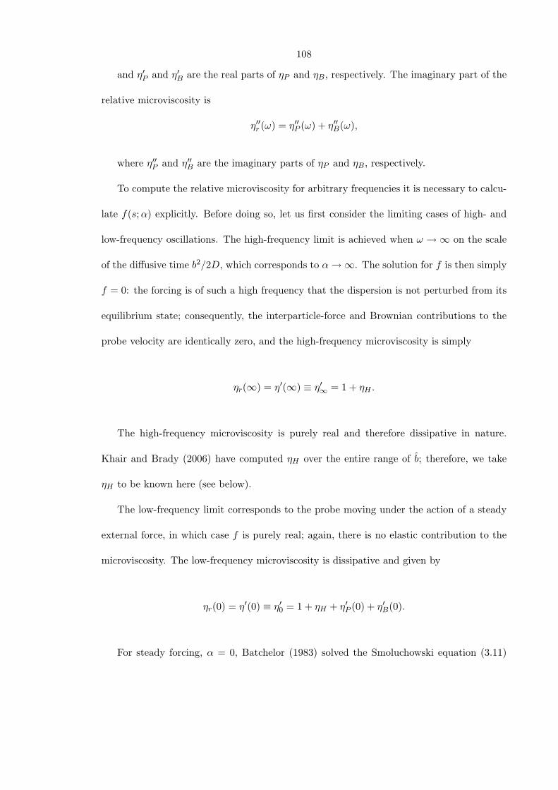
108

and η′P and η′B are the real parts of ηP and ηB, respectively. The imaginary part of the

relative microviscosity is

η′′r (ω) = η′′P (ω) + η′′B(ω),

where η′′P and η′′B are the imaginary parts of ηP and ηB, respectively.

To compute the relative microviscosity for arbitrary frequencies it is necessary to calcu-

late f(s;α) explicitly. Before doing so, let us first consider the limiting cases of high- and

low-frequency oscillations. The high-frequency limit is achieved when ω →∞ on the scale

of the diffusive time b2/2D, which corresponds to α→∞. The solution for f is then simply

f = 0: the forcing is of such a high frequency that the dispersion is not perturbed from its

equilibrium state; consequently, the interparticle-force and Brownian contributions to the

probe velocity are identically zero, and the high-frequency microviscosity is simply

ηr(∞) = η′(∞) ≡ η′∞ = 1 + ηH .

The high-frequency microviscosity is purely real and therefore dissipative in nature.

Khair and Brady (2006) have computed ηH over the entire range of b; therefore, we take

ηH to be known here (see below).

The low-frequency limit corresponds to the probe moving under the action of a steady

external force, in which case f is purely real; again, there is no elastic contribution to the

microviscosity. The low-frequency microviscosity is dissipative and given by

ηr(0) = η′(0) ≡ η′0 = 1 + ηH + η′P (0) + η′B(0).

For steady forcing, α = 0, Batchelor (1983) solved the Smoluchowski equation (3.11)

109

10−3 10−2 10−1 100 101 102

0

0.2

0.4

0.6

0.8

1

1.2

1.4

1.6

1.8

22.1

b/a − 1

(η′ 0 −

1 )

/ φb

Figure 3.1: O(φb) coefficient of the low-frequency microviscosity η′0 versus b = b/a: total(η′0 − 1)/φb, ; hydrodynamic ηH/φb, ; Brownian η′B(0)/φb, ; and interparticle-forceη′P (0)/φb, 4. Data taken from Khair and Brady (2006).

for b ≡ 1 in computing the O(φb) correction to the long-time self-diffusivity. More recently,

Khair and Brady (2006) have solved (3.11) for steady forcing over the entire range of b and

calculated the low-frequency microviscosity η′0. Figure 3.1 plots the O(φb) coefficient of η′0

(i.e. (η′0 − 1)/φb) as a function of b, along with it’s hydrodynamic (ηH/φb), interparticle-

force (η′P (0)/φb), and Brownian (η′B(0)/φb) constituents. (Recall that the high-frequency

microviscosity η′∞ is 1 plus the hydrodynamic microviscosity ηH .) At the extrema of b = 1

(full hydrodynamic interactions) and b → ∞ (no hydrodynamic interactions) we find that

η′0 = 1 + 2.08φb and η′0 = 1 + 2φb, respectively. However, η′0 is a non-monotonic function

of b: it has a minimum of η′0 = 1 + 1.13φb occurring at b ≈ 1.6. The minimum in η′0

arises because b is sufficiently greater than unity, so that the highly resistive hydrodynamic

lubrication interactions (which are present only for b − 1 1) do not hinder the motion

of the probe, but b is also not too large, whence η′0 increases due to the prominent role of

110

the hard-sphere interparticle force (which provides a purely geometrical resistance to the

probe’s motion).

To emphasize the influence of frequency dependent microstructural deformation it is

useful to define reduced microviscosity functions: for the real part of the microviscosity we

define the reduced function as

η′r(ω)− η′∞η′0 − η′∞

=η′P (ω) + η′B(ω)η′P (0) + η′B(0)

, (3.15)

and for the imaginary part of the microviscosity the reduced function is

η′′r (ω)η′0 − η′∞

=η′′P (ω) + η′′B(ω)η′P (0) + η′B(0)

. (3.16)

Both reduced microviscosities are functions of the dimensionless frequency α only; the

explicit volume fraction dependence has been removed by the scaling.

3.4 Connection between microviscosity and self-diffusivity of

the probe particle

Here, we elucidate the intimate relationship between the microviscosity of the dispersion

and the self-diffusivity of the probe particle. Recall, in passive microrheology one measures

the mean-squared displacement of the probe (i.e. its self-diffusivity) and relates this to the

complex modulus of the material through a GSESR. There are several methods (see figure

2 of Waigh 2005) to convert the mean-squared displacement of the probe (a purely real

quantity) into a complex modulus. For example, one can take the Laplace transform of

the mean-squared displacement and apply a Laplace-space GSESR to obtain the (Laplace

111

transformed) relaxation modulus; the complex modulus is then obtained via an analytic

continuation of the Laplace transformed relaxation modulus into Fourier space. Alterna-

tively, one may take the Fourier transform of the mean-squared displacement and apply a

Fourier-space GSESR (Mason 2000), thereby directly obtaining the complex modulus. In

what follows we demonstrate that the small-amplitude oscillatory motion of an active (as

opposed to passive) probe fundamentally relates the microviscosity to self-diffusion.

For sufficiently high frequencies, on the scale of the diffusive time b2/2D, the oscillation

of the probe does not distort the microstructure of the dispersion from its equilibrium state.

Thus, the average velocity of the probe is 〈U1〉 = 〈MUF11 〉eq ·F ext (where 〈· · · 〉eq denotes an

average over the equilibrium microstructure), and the microviscosity is equal to the high-

frequency microviscosity η′∞. On the other hand, the short-time self-diffusivity tensor Ds0 is

defined as kT 〈MUF11 〉eq. For an isotropic equilibrium microstructure Ds

0 = Ds0I; therefore,

the (scalar) short-time self-diffusivity is related to the high-frequency microviscosity via the

identity η′∞ ≡ D/Ds0 (recall, D is the Stokes-Einstein-Sutherland diffusivity, and η′∞ has

already been made dimensionless by the solvent viscosity η).

A probe executing oscillations of lower frequency does disturb the microstructure in its

surroundings. In the small-amplitude regime, to leading order in Peb, the disturbance is pro-

portional to F ext = F eiωt, due to the linearity of the Smoluchowski equation. Consequently,

〈U1〉 is also linearly dependent on F ext, and the complex proportionality constant defines

the frequency-dependent self-diffusivity, Ds(ω), divided by kT . The frequency-dependent

self-diffusivity is equal to the Fourier transform of dDs(t)/dt (Cichocki and Felderhof 1991),

where Ds(t) is the time-dependent self-diffusivity, which is simply the time derivative of the

mean-squared displacement of the probe. Thus, the complex microviscosity is equal to the

inverse of the frequency-dependent self-diffusivity: ηr(ω) ≡ D/Ds(ω).

112

In the limit of zero-frequency oscillations, where the probe moves under a steady external

force, the (purely real) proportionality constant between 〈U1〉 and F ext is the long-time

self-diffusivity, Ds∞, divided by kT . Thus, the zero-frequency or steady-force microviscosity

is related to the long-time self-diffusivity via η′0 ≡ D/Ds∞.

In fact, in the linear-response regime the (Fourier transformed) microstructural evolution

equation for self-diffusion (Brady 1994), at long wavelengths, is identical to that of our

oscillatory probe problem. Note, however, that beyond the linear-response regime there is

no such simple relationship, if indeed a relationship exists at all, between the self-diffusion

problem and the finite-amplitude oscillatory motion of an active probe.

With the above in mind, the scaled transition from low- to high-frequency microviscosity

is equivalent to the scaled transition from long- to short-time self-diffusivity:

ηr(ω)− η′∞η′0 − η′∞

=1/Ds(ω)− 1/Ds

0

1/Ds∞ − 1/Ds

0

,

Thus, in the linear-response regime the connection between the mean-squared displace-

ment (Ds(ω)) and the microviscosity (ηr(ω)) is fundamentally exact by definition; the con-

nection between the microviscosity and the macroviscosity is not obvious, however, and

needs to be addressed.

3.5 Microstructure & microrheology: No hydrodynamic in-

teractions

Before dealing with the complicating effect of hydrodynamic interactions it is instructive to

consider the microstructural deformation problem in their absence. In terms of the excluded-

annulus model neglecting hydrodynamic interactions corresponds to the limit b = b/a→∞:

113

the excluded-volume radius b is much larger than the hydrodynamic radius a. In the absence

of hydrodynamic interactions (G = 1, H = 1, and W = 0) the Smoluchowski equation reads

1s2

d

ds

(s2df

ds

)− 2f

s2− iαf = 0, (3.17)

df

ds= −1 at s = 2, (3.18)

f → 0 as s→∞, (3.19)

and admits the exact solution (Brady 1994)

f =4s2

(1 + z0s/2

1 + z0 + z20/2

)ez0(1−s/2) ,

where z0 = 2(iα)1/2. Without hydrodynamic interactions the Brownian ηB and hydro-

dynamic ηH microviscosity increments are both identically zero, and the relative microvis-

cosity is simply 1 plus the interparticle-force component ηP = 2f(2;α)φb. The solution to

(3.17) for α = 0, corresponding to a steady force on the probe, is f(s; 0) = 4/s2; thus,

the low-frequency microviscosity is η′0 = 1 + 2φb. Of course, in the absence of hydrody-

namic interactions the high-frequency microviscosity is simply equal to solvent viscosity, i.e.

η′∞ = 1.

After a little algebra, the contact value of the structural deformation may be separated

into real and imaginary parts, giving the reduced microviscosity functions

η′r(ω)− η′∞η′0 − η′∞

= <f(2;α) =1 + β + β2

(1 + β)(1 + β2),

and

η′′r (ω)η′0 − η′∞

= −=f(2;α) =β2

(1 + β)(1 + β2),

114

where β = (2α)1/2.

Although we have an exact solution for f(2;α) for arbitrary α, it is useful to examine

the asymptotic limits of small and large α. At small α the contact value of the structural

deformation has the asymptotic form

f(2;α) ∼ 1− (2α)3/2 + (2α)2 − i(2α− (2α)3/2) +O(α3).

The first departure from the steady solution, which is of O(α), is purely imaginary

and therefore elastic in nature. Interestingly, the first frequency correction to the real part

of f(2;α) is O(α3/2), a non-analytic dependence, which is due to singular nature of the

Smoluchowski equation for small α: Brownian diffusion dominates the microstructural de-

formation, except at distances s ∼ O(α−1/2) where it is balanced by unsteadiness/oscillatory

forcing.

In the limit of infinite frequency f = 0, which satisfies the far-field condition (3.19) but

not the no-flux condition at contact (3.18). The perturbation about infinite frequency is

therefore singular, with a boundary layer adjacent to the probe particle in which diffusion

balances oscillatory forcing. Defining the stretched coordinate y = α1/2(s− 2) leads to the

boundary-layer equation d2f/dy2 = if , which has the solution

f =1

(iα)1/2e−i1/2y +

i

2α

(1 + i1/2y

)e−i1/2y +O(α−3/2). (3.20)

To leading order, the real and imaginary parts of f(2;α), and hence ηr, vanish like

α−1/2 as α → ∞. The elastic modulus of the dispersion G′ is related to the imaginary

part of the microviscosity by G′(ω) = ωη′′(ω). A microviscosity decaying as α−1/2 gives

an elastic modulus that diverges as α1/2 at high frequency. The unbounded growth of

115

G′ with α is clearly unphysical, and in § 3.6 it is shown that including full hydrodynamic

interactions (b = 1) removes the divergence. In terms of self-diffusion, the α−1/2 decay in

f(2;α) incorrectly predicts a short-time temporal response proportional to t1/2; again, by

including full hydrodynamic interactions we shall resolve this issue.

It is interesting to compare the complex viscosity obtained from our microrheological

study with that from macrorheology. In macrorheology a colloidal dispersion is subjected

to an oscillatory linear flow of the form Eeiωt, where E is a constant traceless tensor

detailing the flow type (simple shear, elongational etc.). (In macrorheology there is no

probe particle, and all particles have the same hydrodynamic radii a and excluded-volume

radii b). For small-amplitude oscillations, which requires the Peclect number based on the

excluded-volume radius b: Peb = γb2/2D (where γ = |E|), to be much less than unity,

the microstructural deformation is linear in E. Hence, the average stress in the disper-

sion will be strictly proportional to E, and the coefficient of proportionality defines the

complex macroviscosity. In analogy to the complex microviscosity, the real part of the

complex macroviscosity corresponds to viscous dissipation, and the imaginary part cor-

responds to elasticity. There is, however, an important distinction between the micro-

and macro-viscosity: the microstructurally-dependent contribution to the microviscosity

is O(φb), whilst for the macroviscosity it is O(φ2b) (the O(φb) contribution to the relative

macroviscosity is, of course, the single particle Einstein correction 52φ). Nevertheless, using

reduced viscosity functions we are able to scale out the explicit volume fraction dependen-

cies and make a direct comparison between the microstructurally-dependent contributions

to the micro- and macro-viscosities. In figures 3.2 and 3.3 we compare the reduced com-

plex microviscosity to the reduced complex macroviscosity (as computed by Brady 1993)

for dilute dispersions in the absence of hydrodynamic interactions, as a function of the

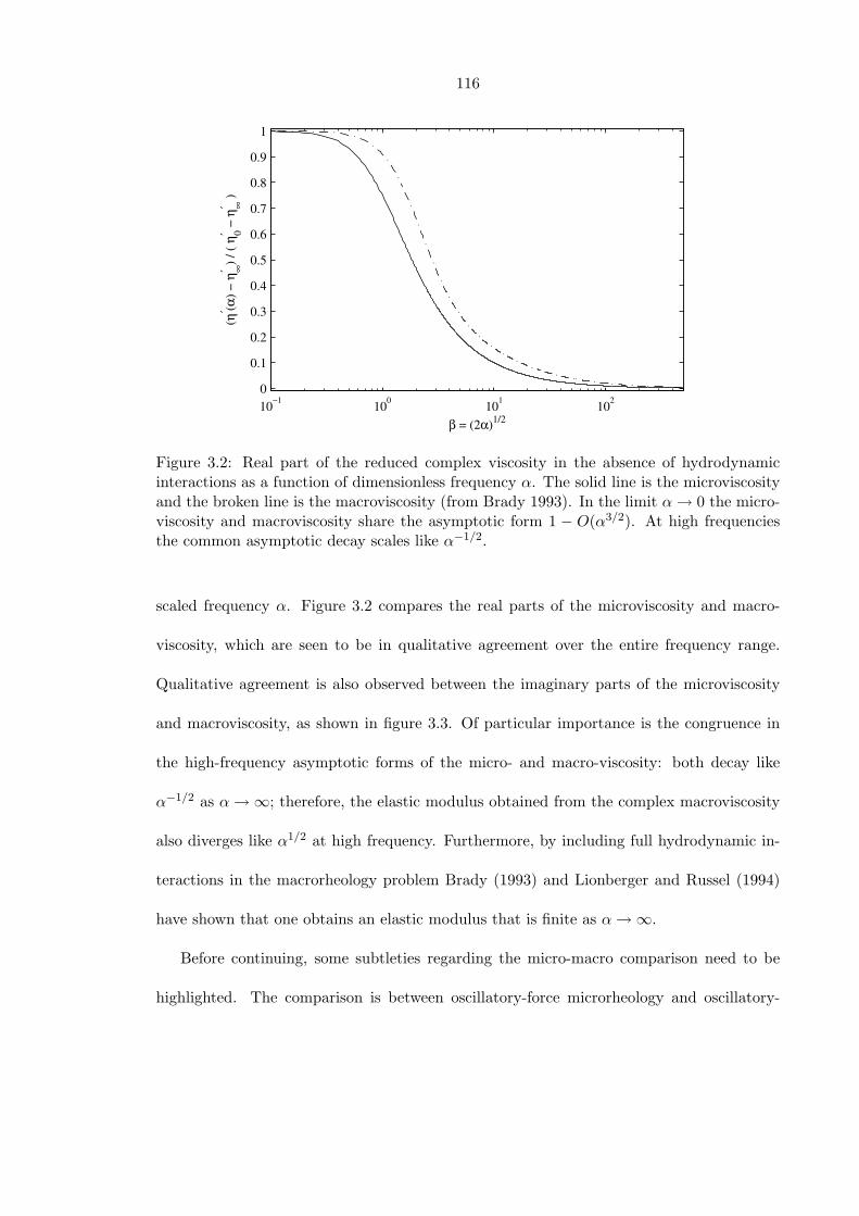
116

10−1 100 101 1020

0.1

0.2

0.3

0.4

0.5

0.6

0.7

0.8

0.9

1

β = (2α)1/2

(η′ (α

) − η

′ ∞) /

( η′ 0 −

η′ ∞

)

Figure 3.2: Real part of the reduced complex viscosity in the absence of hydrodynamicinteractions as a function of dimensionless frequency α. The solid line is the microviscosityand the broken line is the macroviscosity (from Brady 1993). In the limit α→ 0 the micro-viscosity and macroviscosity share the asymptotic form 1 − O(α3/2). At high frequenciesthe common asymptotic decay scales like α−1/2.

scaled frequency α. Figure 3.2 compares the real parts of the microviscosity and macro-

viscosity, which are seen to be in qualitative agreement over the entire frequency range.

Qualitative agreement is also observed between the imaginary parts of the microviscosity

and macroviscosity, as shown in figure 3.3. Of particular importance is the congruence in

the high-frequency asymptotic forms of the micro- and macro-viscosity: both decay like

α−1/2 as α→∞; therefore, the elastic modulus obtained from the complex macroviscosity

also diverges like α1/2 at high frequency. Furthermore, by including full hydrodynamic in-

teractions in the macrorheology problem Brady (1993) and Lionberger and Russel (1994)

have shown that one obtains an elastic modulus that is finite as α→∞.

Before continuing, some subtleties regarding the micro-macro comparison need to be

highlighted. The comparison is between oscillatory-force microrheology and oscillatory-

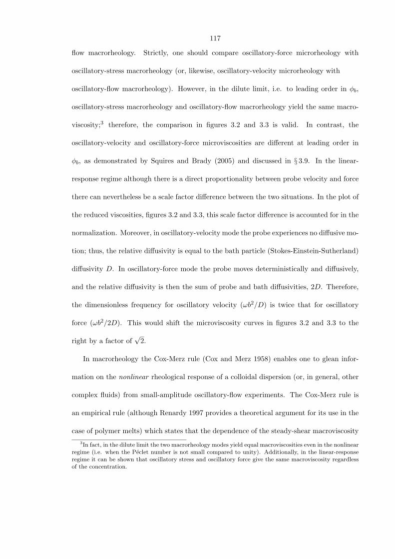
117

flow macrorheology. Strictly, one should compare oscillatory-force microrheology with

oscillatory-stress macrorheology (or, likewise, oscillatory-velocity microrheology with

oscillatory-flow macrorheology). However, in the dilute limit, i.e. to leading order in φb,

oscillatory-stress macrorheology and oscillatory-flow macrorheology yield the same macro-

viscosity;3 therefore, the comparison in figures 3.2 and 3.3 is valid. In contrast, the

oscillatory-velocity and oscillatory-force microviscosities are different at leading order in

φb, as demonstrated by Squires and Brady (2005) and discussed in § 3.9. In the linear-

response regime although there is a direct proportionality between probe velocity and force

there can nevertheless be a scale factor difference between the two situations. In the plot of

the reduced viscosities, figures 3.2 and 3.3, this scale factor difference is accounted for in the

normalization. Moreover, in oscillatory-velocity mode the probe experiences no diffusive mo-

tion; thus, the relative diffusivity is equal to the bath particle (Stokes-Einstein-Sutherland)

diffusivity D. In oscillatory-force mode the probe moves deterministically and diffusively,

and the relative diffusivity is then the sum of probe and bath diffusivities, 2D. Therefore,

the dimensionless frequency for oscillatory velocity (ωb2/D) is twice that for oscillatory

force (ωb2/2D). This would shift the microviscosity curves in figures 3.2 and 3.3 to the

right by a factor of√

2.

In macrorheology the Cox-Merz rule (Cox and Merz 1958) enables one to glean infor-

mation on the nonlinear rheological response of a colloidal dispersion (or, in general, other

complex fluids) from small-amplitude oscillatory-flow experiments. The Cox-Merz rule is

an empirical rule (although Renardy 1997 provides a theoretical argument for its use in the

case of polymer melts) which states that the dependence of the steady-shear macroviscosity3In fact, in the dilute limit the two macrorheology modes yield equal macroviscosities even in the nonlinear

regime (i.e. when the Peclet number is not small compared to unity). Additionally, in the linear-responseregime it can be shown that oscillatory stress and oscillatory force give the same macroviscosity regardlessof the concentration.

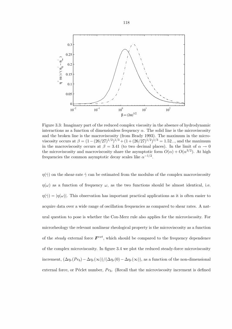
118

10−2 10−1 100 101 1020

0.05

0.1

0.15

0.2

0.25

0.3

β = (2α)1/2

η′′ (α )

/ ( η

0′ − η

∞′ )

Figure 3.3: Imaginary part of the reduced complex viscosity in the absence of hydrodynamicinteractions as a function of dimensionless frequency α. The solid line is the microviscosityand the broken line is the macroviscosity (from Brady 1993). The maximum in the micro-viscosity occurs at β = (1− (26/27)1/2)1/3 +(1+(26/27)1/2)1/3 = 1.52···, and the maximumin the macroviscosity occurs at β = 3.41 (to two decimal places). In the limit of α → 0the microviscosity and macroviscosity share the asymptotic form O(α) +O(α3/2). At highfrequencies the common asymptotic decay scales like α−1/2.

η(γ) on the shear-rate γ can be estimated from the modulus of the complex macroviscosity

η(ω) as a function of frequency ω, as the two functions should be almost identical, i.e.

η(γ) = |η(ω)|. This observation has important practical applications as it is often easier to

acquire data over a wide range of oscillation frequencies as compared to shear rates. A nat-

ural question to pose is whether the Cox-Merz rule also applies for the microviscosity. For

microrheology the relevant nonlinear rheological property is the microviscosity as a function

of the steady external force F ext, which should be compared to the frequency dependence

of the complex microviscosity. In figure 3.4 we plot the reduced steady-force microviscosity

increment, (∆ηr(Peb)−∆ηr(∞))/(∆ηr(0)−∆ηr(∞)), as a function of the non-dimensional

external force, or Peclet number, Peb. (Recall that the microviscosity increment is defined

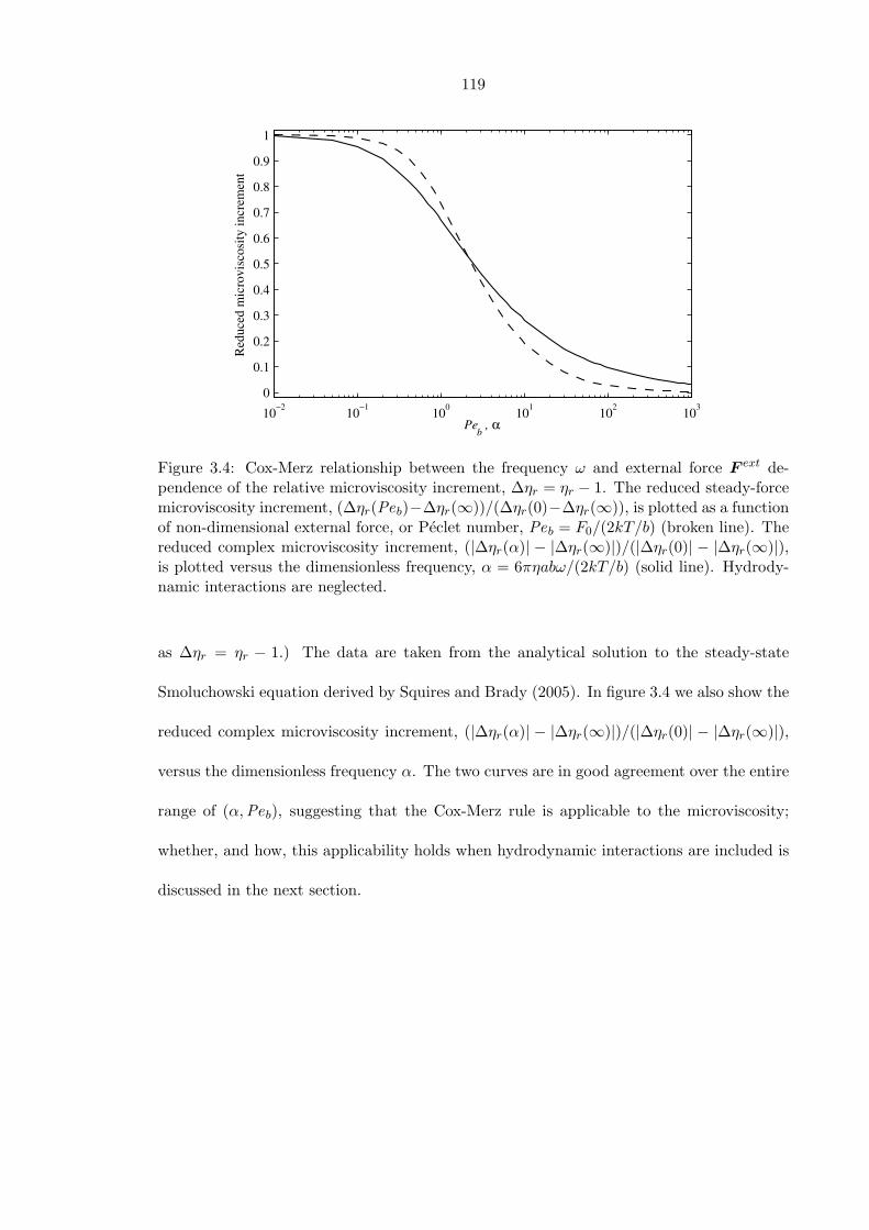
119

10−2 10−1 100 101 102 1030

0.1

0.2

0.3

0.4

0.5

0.6

0.7

0.8

0.9

1

Peb , α

Redu

ced

mic

rovi

scos

ity in

crem

ent

Figure 3.4: Cox-Merz relationship between the frequency ω and external force F ext de-pendence of the relative microviscosity increment, ∆ηr = ηr − 1. The reduced steady-forcemicroviscosity increment, (∆ηr(Peb)−∆ηr(∞))/(∆ηr(0)−∆ηr(∞)), is plotted as a functionof non-dimensional external force, or Peclet number, Peb = F0/(2kT/b) (broken line). Thereduced complex microviscosity increment, (|∆ηr(α)| − |∆ηr(∞)|)/(|∆ηr(0)| − |∆ηr(∞)|),is plotted versus the dimensionless frequency, α = 6πηabω/(2kT/b) (solid line). Hydrody-namic interactions are neglected.

as ∆ηr = ηr − 1.) The data are taken from the analytical solution to the steady-state

Smoluchowski equation derived by Squires and Brady (2005). In figure 3.4 we also show the

reduced complex microviscosity increment, (|∆ηr(α)| − |∆ηr(∞)|)/(|∆ηr(0)| − |∆ηr(∞)|),

versus the dimensionless frequency α. The two curves are in good agreement over the entire

range of (α,Peb), suggesting that the Cox-Merz rule is applicable to the microviscosity;

whether, and how, this applicability holds when hydrodynamic interactions are included is

discussed in the next section.

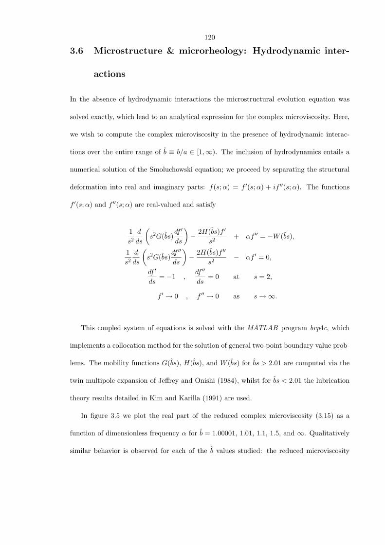
120

3.6 Microstructure & microrheology: Hydrodynamic inter-

actions

In the absence of hydrodynamic interactions the microstructural evolution equation was

solved exactly, which lead to an analytical expression for the complex microviscosity. Here,

we wish to compute the complex microviscosity in the presence of hydrodynamic interac-

tions over the entire range of b ≡ b/a ∈ [1,∞). The inclusion of hydrodynamics entails a

numerical solution of the Smoluchowski equation; we proceed by separating the structural

deformation into real and imaginary parts: f(s;α) = f ′(s;α) + if ′′(s;α). The functions

f ′(s;α) and f ′′(s;α) are real-valued and satisfy

1s2

d

ds

(s2G(bs)

df ′

ds

)− 2H(bs)f ′

s2+ αf ′′ = −W (bs),

1s2

d

ds

(s2G(bs)

df ′′

ds

)− 2H(bs)f ′′

s2− αf ′ = 0,

df ′

ds= −1 ,

df ′′

ds= 0 at s = 2,

f ′ → 0 , f ′′ → 0 as s→∞.

This coupled system of equations is solved with the MATLAB program bvp4c, which

implements a collocation method for the solution of general two-point boundary value prob-

lems. The mobility functions G(bs), H(bs), and W (bs) for bs > 2.01 are computed via the

twin multipole expansion of Jeffrey and Onishi (1984), whilst for bs < 2.01 the lubrication

theory results detailed in Kim and Karilla (1991) are used.

In figure 3.5 we plot the real part of the reduced complex microviscosity (3.15) as a

function of dimensionless frequency α for b = 1.00001, 1.01, 1.1, 1.5, and ∞. Qualitatively

similar behavior is observed for each of the b values studied: the reduced microviscosity

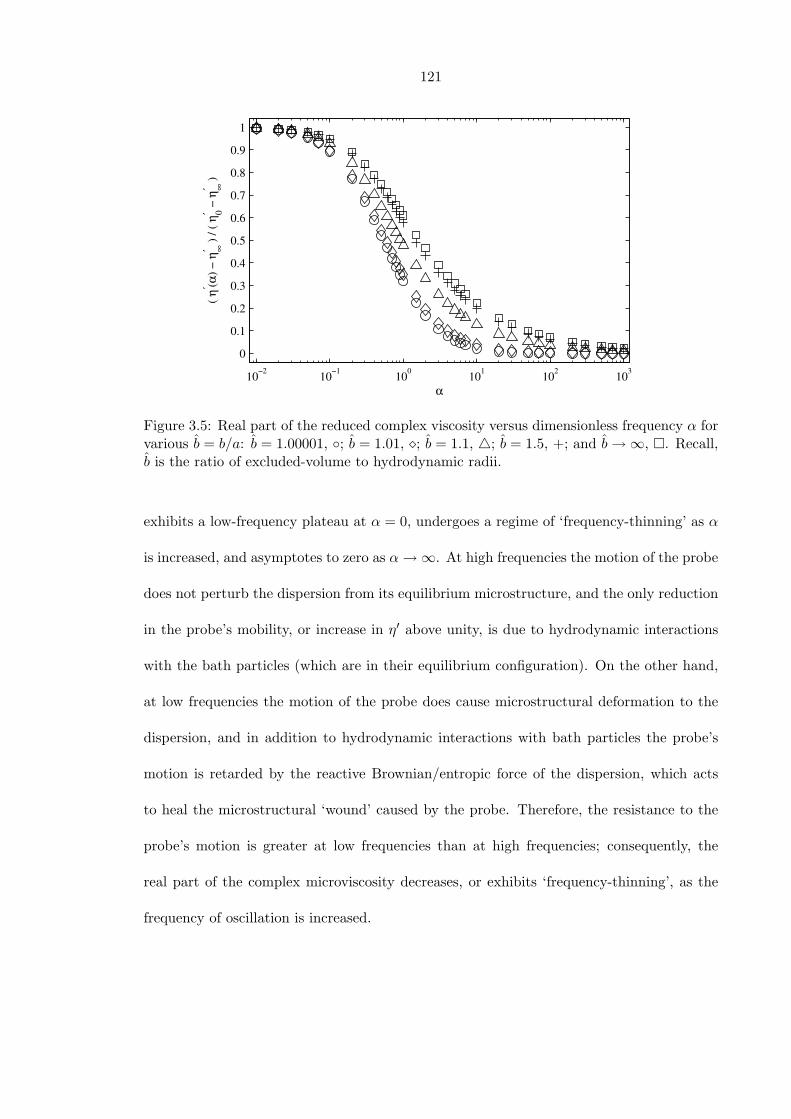
121

10−2 10−1 100 101 102 103

0

0.1

0.2

0.3

0.4

0.5

0.6

0.7

0.8

0.9

1

α

( η′ (α

) − η

′ ∞ )

/ ( η

′ 0 − η

′ ∞ )

Figure 3.5: Real part of the reduced complex viscosity versus dimensionless frequency α forvarious b = b/a: b = 1.00001, ; b = 1.01, ; b = 1.1, 4; b = 1.5, +; and b→∞, . Recall,b is the ratio of excluded-volume to hydrodynamic radii.

exhibits a low-frequency plateau at α = 0, undergoes a regime of ‘frequency-thinning’ as α

is increased, and asymptotes to zero as α→∞. At high frequencies the motion of the probe

does not perturb the dispersion from its equilibrium microstructure, and the only reduction

in the probe’s mobility, or increase in η′ above unity, is due to hydrodynamic interactions

with the bath particles (which are in their equilibrium configuration). On the other hand,

at low frequencies the motion of the probe does cause microstructural deformation to the

dispersion, and in addition to hydrodynamic interactions with bath particles the probe’s

motion is retarded by the reactive Brownian/entropic force of the dispersion, which acts

to heal the microstructural ‘wound’ caused by the probe. Therefore, the resistance to the

probe’s motion is greater at low frequencies than at high frequencies; consequently, the

real part of the complex microviscosity decreases, or exhibits ‘frequency-thinning’, as the

frequency of oscillation is increased.

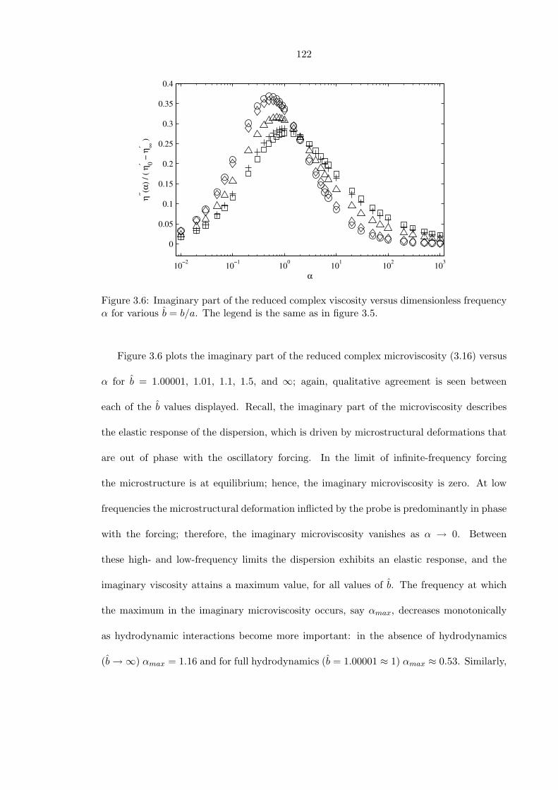
122

10−2 10−1 100 101 102 103

0

0.05

0.1

0.15

0.2

0.25

0.3

0.35

0.4

α

η′′ (α) /

( η′ 0 −

η′ ∞

)

Figure 3.6: Imaginary part of the reduced complex viscosity versus dimensionless frequencyα for various b = b/a. The legend is the same as in figure 3.5.

Figure 3.6 plots the imaginary part of the reduced complex microviscosity (3.16) versus

α for b = 1.00001, 1.01, 1.1, 1.5, and ∞; again, qualitative agreement is seen between

each of the b values displayed. Recall, the imaginary part of the microviscosity describes

the elastic response of the dispersion, which is driven by microstructural deformations that

are out of phase with the oscillatory forcing. In the limit of infinite-frequency forcing

the microstructure is at equilibrium; hence, the imaginary microviscosity is zero. At low

frequencies the microstructural deformation inflicted by the probe is predominantly in phase

with the forcing; therefore, the imaginary microviscosity vanishes as α → 0. Between

these high- and low-frequency limits the dispersion exhibits an elastic response, and the

imaginary viscosity attains a maximum value, for all values of b. The frequency at which

the maximum in the imaginary microviscosity occurs, say αmax, decreases monotonically

as hydrodynamic interactions become more important: in the absence of hydrodynamics

(b→∞) αmax = 1.16 and for full hydrodynamics (b = 1.00001 ≈ 1) αmax ≈ 0.53. Similarly,

123

10−2 10−1 100 101 102 103 104 105

10−4

10−2

100

102

α

G′ (α

) / φ

b = α

η′′ (α

) / φ

b

∼ α1/2

Figure 3.7: Elastic modulus G′(α)/φb = αη′′(α)/φb versus dimensionless frequency α forvarious b = b/a. The legend is the same as in figure 3.5, with the addition of 5 representingb = 1.03.

the ‘half-value’ in the real part of the reduced microviscosity in figure 3.5 (defined as the

frequency, αhalf , at which (η′(αhalf ) − η′∞)/(η′0 − η′∞) = 1/2) decreases monotonically as

hydrodynamics become stronger: in the absence of hydrodynamics αhalf = 1.69 and for

full hydrodynamics αhalf ≈ 0.53. Importantly, both αmax and αhalf are close to unity, for

all values of b. We shall return to this issue in § 3.8 where our theoretical calculations are

compared to experimental data.

From the discussion above, one might be lead to believe that hydrodynamic interactions

play only a quantitative role in the viscoelasticity of the dispersion; however, as we shall

see below, this is not the case.

Further insight into the effect of hydrodynamic interactions on the viscoelasticity of

the dispersion may be acquired by examination of the elastic modulus G′(α). Recall, in

the absence of hydrodynamic interactions G′ ∼ α1/2 as α → ∞. In figure 3.7 the elastic

124

modulus is plotted as a function of α for b = 1.00001, 1.01, 1.03, 1.1, 1.5, and ∞. With the

exception of b = 1.00001, it is seen that G′ ∼ α1/2 as α→∞, for all values of b shown. To

understand this behavior it is necessary to examine the high-frequency asymptotics of the

Smoluchowski equation.

We proceed with a regular perturbation expansion of the structural deformation in in-

verse powers of α. To leading order the Smoluchowski equation (3.11) reflects a balance be-

tween oscillatory forcing and advection, with the asymptotic solution f ≡ F = −iW (bs)/α.

At large distances W (bs) ∼ O(bs)−5; thus, F satisfies the zero deformation condition (3.13),

but does not satisfy the no-flux boundary condition at contact (3.12). The perturbation

about infinite frequency is singular: near contact there exists a boundary layer of O(α−1/2)

in which (radial) Brownian diffusion balances unsteady effects. In appendix 3.A we show

that in the boundary layer the structural deformation is

f(y;α) =(G0

iα

)1/2

e−(i/G0)1/2y +i

4α(2G0 +G1)

(1 +

(i

G0

)1/2

y

)e−(i/G0)1/2y

+G1

4αG0y2e−(i/G0)1/2y − iW0

α+O(α−3/2),

where y = α1/2(s− 2) is a boundary-layer coordinate, G0 = G(2b), G1 = dG/ds|2b, and

W0 = W (2b). As y → ∞, f → −iW0/α, which is precisely the inner limit of the outer

solution F = −iW (bs)/α. After a little work (again, see Appendix 3.A for the details) the

interparticle-force G′P and Brownian G′

B contributions to the elastic modulus G′ are found

as

G′P

φb=

(2G3

0α)1/2 −G0

(G0 +

G1

2− 2W0

)+O(α−1/2), (3.21)

G′B

φb= 2W0G0 +

12

∫ ∞

2[W (bs)]2s2ds+O(α−1/2). (3.22)

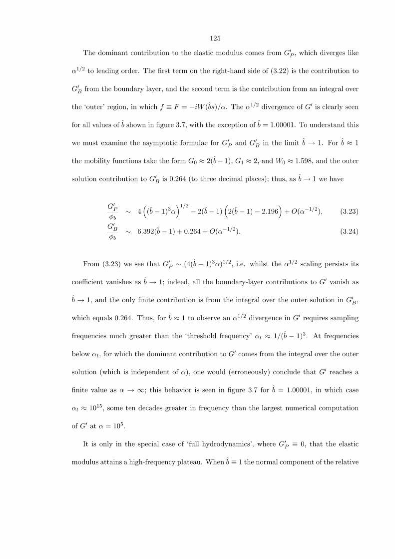
125

The dominant contribution to the elastic modulus comes from G′P , which diverges like

α1/2 to leading order. The first term on the right-hand side of (3.22) is the contribution to

G′B from the boundary layer, and the second term is the contribution from an integral over

the ‘outer’ region, in which f ≡ F = −iW (bs)/α. The α1/2 divergence of G′ is clearly seen

for all values of b shown in figure 3.7, with the exception of b = 1.00001. To understand this

we must examine the asymptotic formulae for G′P and G′

B in the limit b → 1. For b ≈ 1

the mobility functions take the form G0 ≈ 2(b− 1), G1 ≈ 2, and W0 ≈ 1.598, and the outer

solution contribution to G′B is 0.264 (to three decimal places); thus, as b→ 1 we have

G′P

φb∼ 4

((b− 1)3α

)1/2− 2(b− 1)

(2(b− 1)− 2.196

)+O(α−1/2), (3.23)

G′B

φb∼ 6.392(b− 1) + 0.264 +O(α−1/2). (3.24)

From (3.23) we see that G′P ∼ (4(b − 1)3α)1/2, i.e. whilst the α1/2 scaling persists its

coefficient vanishes as b → 1; indeed, all the boundary-layer contributions to G′ vanish as

b → 1, and the only finite contribution is from the integral over the outer solution in G′B,

which equals 0.264. Thus, for b ≈ 1 to observe an α1/2 divergence in G′ requires sampling

frequencies much greater than the ‘threshold frequency’ αt ≈ 1/(b − 1)3. At frequencies

below αt, for which the dominant contribution to G′ comes from the integral over the outer

solution (which is independent of α), one would (erroneously) conclude that G′ reaches a

finite value as α → ∞; this behavior is seen in figure 3.7 for b = 1.00001, in which case

αt ≈ 1015, some ten decades greater in frequency than the largest numerical computation

of G′ at α = 105.

It is only in the special case of ‘full hydrodynamics’, where G′P ≡ 0, that the elastic

modulus attains a high-frequency plateau. When b ≡ 1 the normal component of the relative

126

velocity between the probe and bath particle is zero at contact; consequently, the inner

boundary condition on the Smoluchowski equation is s·D ·∇g = 0, and for small-amplitude

forcing this implies (s − 2)df/ds = 0 at s = 2. The outer solution of f ≡ F = −iW (s)/α

is uniformly valid, i.e. it satisfies the boundary condition at s = 2; hence, there is no

boundary layer near contact. This is consistent with (3.23) and (3.24), which indicate

that the boundary-layer contributions to G′ vanish as b → 1. The numerical value of the

high-frequency plateau for b ≡ 1, denoted as G′∞, is

G′∞ = −αφb

2

∫ ∞

2W (s)=f(s;α)s2ds =

φb

2

∫ ∞

2[W (s)]2s2ds = 0.264φb.

Theoretical macrorheology studies by Brady (1993) and Lionberger and Russel (1994)

find that the elastic modulus attains a high-frequency plateau for b ≡ 1, in agreement with

our results; in the absence of hydrodynamic interactions (b → ∞) they both observe that

G′ grows like α1/2 as α → ∞, in accordance with the findings of § 3.5. Between these

two limiting cases it is expected that the elastic modulus obtained from macrorheology

should also diverge like α1/2 as α → ∞ (or, more precisely, for frequencies greater than

a macrorheology threshold frequency analogous to αt) as per the microviscosity (3.23).

However, at the present time, the numerical solution of the macrorheology Smoluchowski

equation at finite b has yet to be determined.

The divergence ofG′ as α→∞ originates from the excluded-annulus model of interparticle-

force interactions, which implements a hard-sphere repulsion between the probe and a bath

particle, acting at a distance b greater than the true radius a of the probe. If the colloidal

particles experience a soft interparticle-force interaction Brady (1993) has shown that the

elastic modulus determined from macrorheology attains a high-frequency plateau. One

127

should observe an analogous plateau in the microrheological elastic modulus, although we

leave this for future study. Finally, we note the implications for self-diffusivity: for full hy-

drodynamics the 1/α decay of f(y;α) predicts a short-time temporal response proportional

to t.

In § 3.5 (see also figure 3.4) we demonstrated that in the absence of hydrodynamic inter-

actions the microviscosity obeys, to a good degree, the Cox-Merz rule. (Recall, the Cox-Merz

rule states η(F ext) = |η(ω)|, where η(F ext) is the nonlinear microviscosity obtained from

a steady-force experiment, and |η(ω)| is the linear microviscosity from an small-amplitude,

oscillatory-force experiment.) In the presence of hydrodynamic interactions the application

of the Cox-Merz rule needs to be modified. In steady-force microrheology the microviscos-

ity increment, ∆ηr = ηr − 1, is a sum of hydrodynamic, Brownian, and interparticle-force

contributions: the hydrodynamic contribution is a monotonically increasing function of the

non-dimensional force (or Peclet number, Peb), whilst the Brownian and interparticle-force

contributions are monotonically decreasing functions of Peb (Khair and Brady 2006). If hy-

drodynamic interactions are sufficiently strong, i.e. b ≈ 1, the increase in the hydrodynamic

contribution outweighs the decrease in the Brownian and interparticle-force contributions,

and the microviscosity ‘force-thickens’, in analogy to macrorheological shear-thickening, at

large Peb. For small-amplitude oscillatory-force experiments the microviscosity increment

is again comprised of hydrodynamic, Brownian, and interparticle-force constituents; how-

ever, the hydrodynamic contribution, to leading order in the oscillation amplitude Peb, is

not a function of the oscillation frequency and merely sets the bath particle contribution to

the high-frequency dynamic microviscosity. The Brownian and interparticle-force microvis-

cosity contributions are, of course, frequency-dependent. Therefore, when hydrodynamic

interactions are present the Cox-Merz is understood to mean ηT (F ext) = |ηT (ω)|, where the

128

subscript T denotes the thermodynamic (i.e. Brownian plus interparticle-force) contribution

to the microviscosity.

One can measure ηT via so-called stress-jump (or flow-cessation) experiments. In

macrorheological stress-jump experiments the dispersion is sheared at a constant rate until

a steady-state microstructure is attained (in which the colloidal particles are subject to

hydrodynamic and thermodynamic forces), and the shear is then stopped suddenly: the

hydrodynamic contribution to the macroviscosity vanishes instantly, allowing one to isolate

the thermodynamic contribution ηT (which decays on the diffusive microstructural relax-

ation time scale). It is possible to formulate a microrheological analog of the stress-jump

experiment (as discussed in § 3.9), so that one may verify the Cox-Merz relationship with

experimental microviscosity data.

In figure 3.8 we plot the reduced steady-force microviscosity increment, (∆T ηr(Peb) −

∆T ηr(∞))/(∆T ηr(0)−∆T ηr(∞)), as a function of Peb; here, ∆T ηr(Peb) = ηr(Peb)− (1 +

ηH(Peb)) is the thermodynamic contribution to the microviscosity increment. The data are

taken from the numerical solution of the Smoluchowski equation by Khair and Brady (2006).

The reduced complex microviscosity increment, (|∆T ηr(α)| − |∆T ηr(∞)|)/(|∆T ηr(0)| −

|∆T ηr(∞)|), is also plotted in figure 3.8, versus the dimensionless frequency α. For both

sets of data b = 1.00001. Reasonable agreement (the half-value, αhalf , of the steady-force

increment is approximately three times that of the complex increment) between the steady-

force microviscosity increment and the complex microviscosity increment is observed over

the entire range of (α,Peb), indicating that the Cox-Merz rule may be applicable to the

(thermodynamic contribution of the) microviscosity when hydrodynamic interactions are

present.

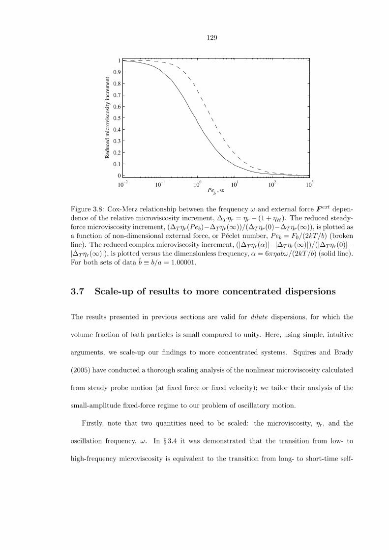
129

10−2 10−1 100 101 102 1030

0.1

0.2

0.3

0.4

0.5

0.6

0.7

0.8

0.9

1

Peb , α

Redu

ced

mic

rovi

scos

ity in

crem

ent

Figure 3.8: Cox-Merz relationship between the frequency ω and external force F ext depen-dence of the relative microviscosity increment, ∆T ηr = ηr − (1 + ηH). The reduced steady-force microviscosity increment, (∆T ηr(Peb)−∆T ηr(∞))/(∆T ηr(0)−∆T ηr(∞)), is plotted asa function of non-dimensional external force, or Peclet number, Peb = F0/(2kT/b) (brokenline). The reduced complex microviscosity increment, (|∆T ηr(α)|−|∆T ηr(∞)|)/(|∆T ηr(0)|−|∆T ηr(∞)|), is plotted versus the dimensionless frequency, α = 6πηabω/(2kT/b) (solid line).For both sets of data b ≡ b/a = 1.00001.

3.7 Scale-up of results to more concentrated dispersions

The results presented in previous sections are valid for dilute dispersions, for which the

volume fraction of bath particles is small compared to unity. Here, using simple, intuitive

arguments, we scale-up our findings to more concentrated systems. Squires and Brady

(2005) have conducted a thorough scaling analysis of the nonlinear microviscosity calculated

from steady probe motion (at fixed force or fixed velocity); we tailor their analysis of the

small-amplitude fixed-force regime to our problem of oscillatory motion.

Firstly, note that two quantities need to be scaled: the microviscosity, ηr, and the

oscillation frequency, ω. In § 3.4 it was demonstrated that the transition from low- to

high-frequency microviscosity is equivalent to the transition from long- to short-time self-

130

diffusivity. The self-diffusivity transition may be expressed in dimensional form as (Cichocki

and Felderhof 1991)

Ds∞ −Ds

0 =13

∫ ∞

0〈v(t) · v(0)〉dt,

where 〈v(t) · v(0)〉 is the velocity autocorrelation function. Here, 〈· · · 〉 denotes an

ensemble average over all particles in the dispersion and v(t) is the regular part of the

velocity of a ‘tagged’ particle (that is, only the part which fluctuates due to microstructural

fluctuations caused by Brownian motion) measured on the diffusive, or Smoluchowski, time

scale b2/D. The ‘relaxation’ time scale characterizing the self-diffusivity transition is simply

defined by

τD(φb) =

∫∞0 〈tv(t) · v(0)〉dt∫∞0 〈v(t) · v(0)〉dt

.

We define a dimensionless oscillation frequency α∗(φb) = ωτD(φb). In the dilute limit,

φb 1, and in the absence of hydrodynamic interactions, b → ∞, Cichocki and Felderhof

(1993) calculate DτD/b2 = 1. Therefore, α∗(φb 1) = 2 × (ωb2/2D), which is a factor of

two greater than our ‘naive’ scaling of α = ωb2/2D (see equation (3.2)). Little appears to

be known about the behavior of τD beyond the dilute limit. The Brownian Dynamics (BD)

simulations of Cichocki and Hinsen (1992) suggest that DτD/b2 decreases with increasing

φb until φb ≈ 0.46, where it attains a minimum value of DτD/b2 ≈ 0.06, and then increases.

Unfortunately, Cichocki and Hinsen (1992) do not present data beyond φb = 0.50, and it is

not known how τD behaves as the limit of random close packing, φm ≈ 0.63, is approached.

Intuitively, one would expect that τD diverges as φb → φm: a particle becomes trapped in a

‘cage’ formed by other particles and can only escape the cage (and hence lose correlation with

its initial velocity) on times much larger than b2/D. With full hydrodynamic interactions,

b = 1, all that is known about τD, to our knowledge, is the dilute-limit resultDτD/b2 = 1.868

131

(Cichocki and Felderhof 1993). In § 3.8, where our theoretical calculations are compared to

experimental micro- and macro-viscosity data, we propose a simple model for the volume

fraction dependence of τD.

Finally, the microviscosity itself must be scaled, or, more precisely, the contribution

to the microviscosity arising from microstructural deformations ∆η ≡ ηr − η′∞ (recall, the

high-frequency dynamic microviscosity η′∞ is a function of the equilibrium microstructure).

As mentioned above, for small-amplitude forcing the average velocity of the probe is pro-

portional to the long-time self-diffusivity; thus, the appropriate scale for ∆η is D/Ds∞.

Brady (1994) has shown that the long-time self-diffusivity may be approximated as Ds∞ =

Ds0 × Ds,nohydro

∞ , where Ds,nohydro∞ is the dimensionless long-time self-diffusivity in the ab-

sence of hydrodynamic interactions; furthermore, Brady (1994) notes that Ds,nohydro∞ scales

approximately like 1/φbgeq(2;φb), where geq(2;φb) is the contact-value of the equilibrium

pair-distribution function (which may be obtained from the Carnahan-Starling equation of

state).

Putting this together suggests the microviscosity to scale like

∆η ∼ D

Ds∞

Υ(α∗; b) ≈ φbgeq(2;φb)Ds

0/DΥ(α∗; b),

where the dimensionless (complex) function Υ(α∗; b) details the frequency response for

a particular value of b. Interestingly, starting from the N -particle Smoluchowski equa-

tion, Brady (1993) demonstrates that the macroviscosity scales in the same manner as the

microviscosity (aside from an extra factor of φb for the macroviscosity).

132

3.8 Comparison with experimental data

In § 3.5 (see also figures 3.2 and 3.3) we showed in the dilute limit and in the absence of

hydrodynamic interactions that the complex microviscosity compares favorably with the

complex macroviscosity over the entire range of oscillation frequencies. Here, with the

aid of the scaling arguements developed in § 3.7, we compare our microviscosity results to

experimental micro- and macro-viscosity data for concentrated dispersions.

The appropriate time scale for macroviscoelastic response arises from consideration of

the transition from low- to high-frequency macroviscosity, which is given by the following

dimensional Green-Kubo formula (Nagele and Bergenholtz 1998)

η′0 − η′∞ =V

kT

∫ ∞

0〈σT

xy(t)σTxy(0)〉dt,

where V is the volume, 〈σTxy(t)σ

Txy(0)〉 is the shear stress autocorrelation function, and

σTxy(t) denotes the instantaneous thermodynamic shear stress (due to interparticle-forces

and/or Brownian diffusion) arising from fluctuations in the dispersion microstructure about

its equilibrium configuration. (The subscript xy is used for definiteness, but since there is

no preferred direction at equilibrium we could have used xz or yz.) In analogy to τD, we

define a macroviscosity relaxation time

τη(φb) =

∫∞0 〈tσT

xy(t)σTxy(0)〉dt∫∞

0 〈σTxy(t)σT

xy(0)〉dt.

In the dilute limit and in the absence of hydrodynamic interactions Dτη/b2 = 2/9

(Cichocki and Felderhof 1993). For higher concentrations much more is known about τη as

compared to τD. The mode coupling theory (MCT) calculations of Banchio et al. (1999)

133

show that τη decreases on increasing φb (MCT predicts Dτη/b2 = 0.19 in the dilute limit)

until φb ≈ 0.3, at which point it attains a minimum of Dτη/b2 ≈ 0.08. This initial decrease

in τη is due to the increasing number of collisions as φb increases past the dilute limit, which

leads to faster relaxation of the shear stress. Beyond φb ≈ 0.3, τη increases and diverges in

the limit φb → φm. In analogy to τD, the increase in τη for φb > 0.3 is due to the caging of

particles in concentrated dispersions, which leads to a slower relaxation of the shear stress.

The MCT description of τη as a function of φb is confirmed by the BD study of Foss and

Brady (2000); interestingly, both Foss and Brady (2000) and Banchio et al. (1999) find that

the product Ds,nohydro∞ (φb)τη(φb)/b2 is approximately constant over a wide range of φb. In

particular, τη(φb) scales like b2/Ds,nohydro∞ (φb) as φb → φm (here, Ds,nohydro

∞ = D×Ds,nohydro∞

is the dimensional long-time self-diffusivity in the absence of hydrodynamic interactions).

With full hydrodynamic interactions and in the dilute limit Dτη/b2 = 0.4892 (Cichocki

and Felderhof 1993), which is approximately double the value of Dτη/b2 in the absence of

hydrodynamic interactions. Beyond the dilute limit nothing, to our knowledge, is known

theoretically about τη in the presence of hydrodynamic interactions, although Van der Werff

et al. (1989) have measured this quantity experimentally. The ‘simplest’ way to account for

the effect of hydrodynamic interactions on τη (and, for that matter, τD) is in an averaged, or

mean-field like, approach by replacing the solvent viscosity with the high-frequency dynamic

macroviscosity: it is as if two particles are in a suspending fluid of effective viscosity η′∞.

As the high-frequency dynamic macroviscosity is inversely proportional to the short-time

self-diffusivity (Brady 1994) one may equivalently multiply Ds,nohydro∞ by Ds

0/D; thus, in the

presence of hydrodynamic interactions we propose that τη(φb) scales like b2/Ds∞(φb), where

Ds∞ = Ds

0 × Ds,nohydro∞ is the long-time self-diffusivity in the presence of hydrodynamic

interactions. To test the accuracy of this assumption one could calculate τη from Stokesian

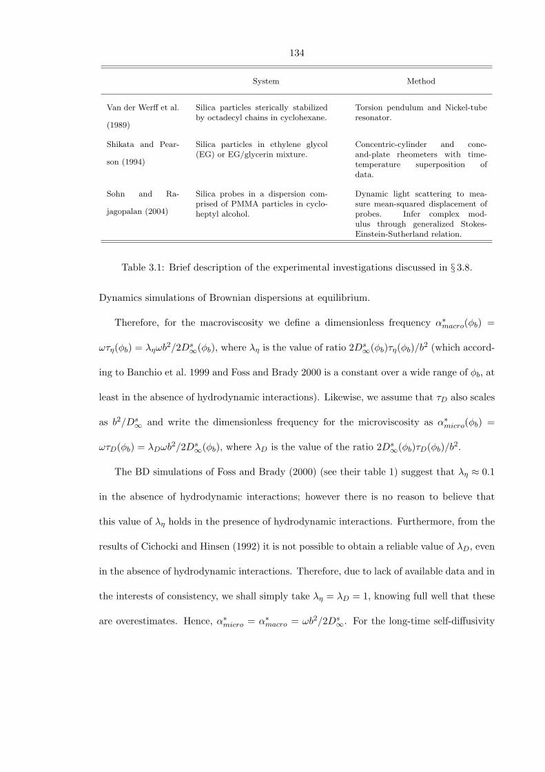
134

System Method

Van der Werff et al.

(1989)

Silica particles sterically stabilizedby octadecyl chains in cyclohexane.

Torsion pendulum and Nickel-tuberesonator.

Shikata and Pear-

son (1994)

Silica particles in ethylene glycol(EG) or EG/glycerin mixture.

Concentric-cylinder and cone-and-plate rheometers with time-temperature superposition ofdata.

Sohn and Ra-

jagopalan (2004)

Silica probes in a dispersion com-prised of PMMA particles in cyclo-heptyl alcohol.

Dynamic light scattering to mea-sure mean-squared displacement ofprobes. Infer complex mod-ulus through generalized Stokes-Einstein-Sutherland relation.

Table 3.1: Brief description of the experimental investigations discussed in § 3.8.

Dynamics simulations of Brownian dispersions at equilibrium.

Therefore, for the macroviscosity we define a dimensionless frequency α∗macro(φb) =

ωτη(φb) = ληωb2/2Ds

∞(φb), where λη is the value of ratio 2Ds∞(φb)τη(φb)/b2 (which accord-

ing to Banchio et al. 1999 and Foss and Brady 2000 is a constant over a wide range of φb, at

least in the absence of hydrodynamic interactions). Likewise, we assume that τD also scales

as b2/Ds∞ and write the dimensionless frequency for the microviscosity as α∗micro(φb) =

ωτD(φb) = λDωb2/2Ds

∞(φb), where λD is the value of the ratio 2Ds∞(φb)τD(φb)/b2.

The BD simulations of Foss and Brady (2000) (see their table 1) suggest that λη ≈ 0.1

in the absence of hydrodynamic interactions; however there is no reason to believe that

this value of λη holds in the presence of hydrodynamic interactions. Furthermore, from the

results of Cichocki and Hinsen (1992) it is not possible to obtain a reliable value of λD, even

in the absence of hydrodynamic interactions. Therefore, due to lack of available data and in

the interests of consistency, we shall simply take λη = λD = 1, knowing full well that these

are overestimates. Hence, α∗micro = α∗macro = ωb2/2Ds∞. For the long-time self-diffusivity

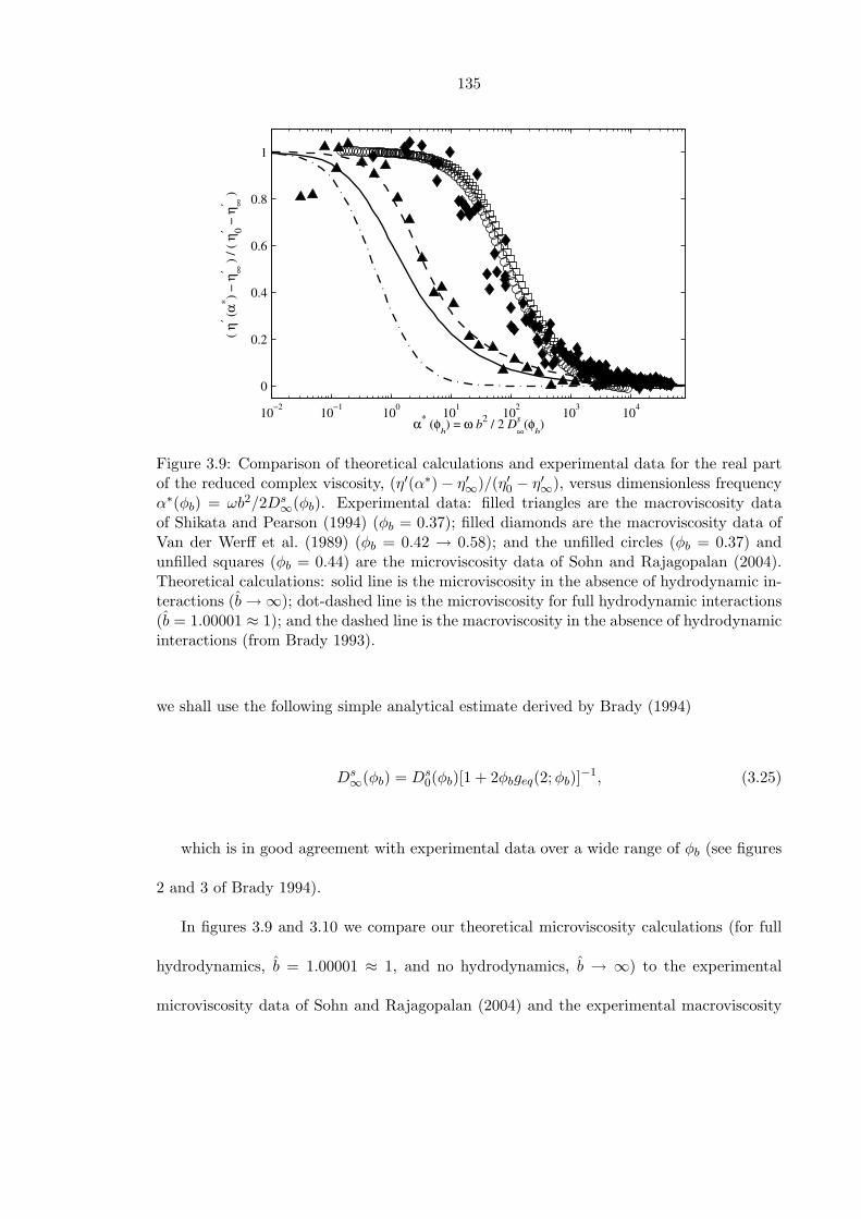
135

10−2 10−1 100 101 102 103 104

0

0.2

0.4

0.6

0.8

1

α* (φb) = ω b2 / 2 Ds∞(φb)

( η′ (α

* ) − η

′ ∞ )

/ ( η

′ 0 − η

′ ∞ )

Figure 3.9: Comparison of theoretical calculations and experimental data for the real partof the reduced complex viscosity, (η′(α∗)− η′∞)/(η′0 − η′∞), versus dimensionless frequencyα∗(φb) = ωb2/2Ds

∞(φb). Experimental data: filled triangles are the macroviscosity dataof Shikata and Pearson (1994) (φb = 0.37); filled diamonds are the macroviscosity data ofVan der Werff et al. (1989) (φb = 0.42 → 0.58); and the unfilled circles (φb = 0.37) andunfilled squares (φb = 0.44) are the microviscosity data of Sohn and Rajagopalan (2004).Theoretical calculations: solid line is the microviscosity in the absence of hydrodynamic in-teractions (b→∞); dot-dashed line is the microviscosity for full hydrodynamic interactions(b = 1.00001 ≈ 1); and the dashed line is the macroviscosity in the absence of hydrodynamicinteractions (from Brady 1993).

we shall use the following simple analytical estimate derived by Brady (1994)

Ds∞(φb) = Ds

0(φb)[1 + 2φbgeq(2;φb)]−1, (3.25)

which is in good agreement with experimental data over a wide range of φb (see figures

2 and 3 of Brady 1994).

In figures 3.9 and 3.10 we compare our theoretical microviscosity calculations (for full

hydrodynamics, b = 1.00001 ≈ 1, and no hydrodynamics, b → ∞) to the experimental

microviscosity data of Sohn and Rajagopalan (2004) and the experimental macroviscosity

136

data of Van der Werff et al. (1989) and Shikata and Pearson (1994) (see table 3.1 for a

brief description of each experimental study). Figure 3.9 plots the real part of the reduced

viscosity, (η′(α∗)−η′∞)/(η′0−η′∞), versus dimensionless frequency, α∗ = ωb2/2Ds∞. Although

the shape of each experimental reduced viscosity data set as a function of α∗ is in qualitative

agreement with our theoretical microviscosity calculations, the experimental data are shifted

to higher α∗ as compared to the theoretical curves: for the data of Van der Werff et al.

(1989) and Sohn and Rajagopalan (2004) the shift is by approximately two decades in α∗.

One should, however, not be alarmed by this shift of the experimental data since in the

comparison, due to the lack of available data, we took λη = λD = 1. Van der Werff et al.

(1989) observe that G′(ω) ∼ ω1/2 at high frequencies, which indicates that short-range

hydrodynamic lubrication interactions may not be important in their dispersions; the BD

simulations of Foss and Brady (2000) suggest that λη ≈ 0.1, which would shift the data of

Van der Werff et al. (1989) a decade lower in α∗, as compared to figure 3.9. Furthermore, if

lubrication interactions are not present the simple formula (3.25) underestimates the long-

time self-diffusivity, and this may also contribute to the discrepancy between their data and

the theoretical curves. Similarly, before drawing conclusions concerning the comparison of

our microviscosity calculations with the data of Shikata and Pearson (1994) and Sohn and

Rajagopalan (2004), which both exhibit a high-frequency plateau in the elastic modulus, one

needs to calculate λη and λD in the presence of full hydrodynamic interactions. Additionally,

Sohn and Rajagopalan (2004) used probe particles approximately twice as large as their

bath particles; therefore, properly, one should define a dimensionless frequency for their data

as ωb2/Dr∞, where Dr

∞ is the long-time relative diffusivity, rather than ωb2/Ds∞. Whilst

Dr∞ and Ds

∞ should share the same dependence on bath particle concentration, Dr∞ is also

a function of the ratio of probe size to bath particle size. Furthermore, the theoretical

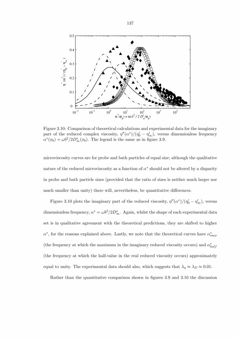
137

10−2 10−1 100 101 102 103 1040

0.1

0.2

0.3

0.4

0.5

α*(φb) = ω b2 / 2 Ds∞(φb)

η′′ (α* ) /

(η′ 0 −

η′ ∞

)

Figure 3.10: Comparison of theoretical calculations and experimental data for the imaginarypart of the reduced complex viscosity, η′′(α∗)/(η′0 − η′∞), versus dimensionless frequencyα∗(φb) = ωb2/2Ds

∞(φb). The legend is the same as in figure 3.9.

microviscosity curves are for probe and bath particles of equal size; although the qualitative

nature of the reduced microviscosity as a function of α∗ should not be altered by a disparity

in probe and bath particle sizes (provided that the ratio of sizes is neither much larger nor

much smaller than unity) there will, nevertheless, be quantitative differences.

Figure 3.10 plots the imaginary part of the reduced viscosity, η′′(α∗)/(η′0 − η′∞), versus

dimensionless frequency, α∗ = ωb2/2Ds∞. Again, whilst the shape of each experimental data

set is in qualitative agreement with the theoretical predictions, they are shifted to higher

α∗, for the reasons explained above. Lastly, we note that the theoretical curves have α∗max

(the frequency at which the maximum in the imaginary reduced viscosity occurs) and α∗half

(the frequency at which the half-value in the real reduced viscosity occurs) approximately

equal to unity. The experimental data should also, which suggests that λη ≈ λD ≈ 0.01.

Rather than the quantitative comparison shown in figures 3.9 and 3.10 the discussion

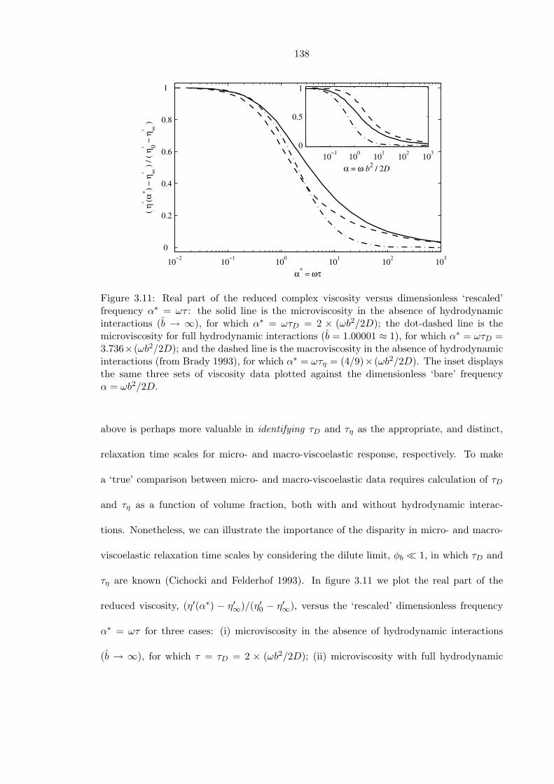
138

10−2 10−1 100 101 102 1030

0.2

0.4

0.6

0.8

1

α* = ωτ

( η′ (α

* ) − η

′ ∞ )

/ ( η

′ 0 − η

′ ∞ )

10−1 100 101 102 1030

0.5

1

α = ω b2 / 2D

Figure 3.11: Real part of the reduced complex viscosity versus dimensionless ‘rescaled’frequency α∗ = ωτ : the solid line is the microviscosity in the absence of hydrodynamicinteractions (b → ∞), for which α∗ = ωτD = 2 × (ωb2/2D); the dot-dashed line is themicroviscosity for full hydrodynamic interactions (b = 1.00001 ≈ 1), for which α∗ = ωτD =3.736×(ωb2/2D); and the dashed line is the macroviscosity in the absence of hydrodynamicinteractions (from Brady 1993), for which α∗ = ωτη = (4/9)× (ωb2/2D). The inset displaysthe same three sets of viscosity data plotted against the dimensionless ‘bare’ frequencyα = ωb2/2D.

above is perhaps more valuable in identifying τD and τη as the appropriate, and distinct,

relaxation time scales for micro- and macro-viscoelastic response, respectively. To make

a ‘true’ comparison between micro- and macro-viscoelastic data requires calculation of τD

and τη as a function of volume fraction, both with and without hydrodynamic interac-

tions. Nonetheless, we can illustrate the importance of the disparity in micro- and macro-

viscoelastic relaxation time scales by considering the dilute limit, φb 1, in which τD and

τη are known (Cichocki and Felderhof 1993). In figure 3.11 we plot the real part of the

reduced viscosity, (η′(α∗) − η′∞)/(η′0 − η′∞), versus the ‘rescaled’ dimensionless frequency

α∗ = ωτ for three cases: (i) microviscosity in the absence of hydrodynamic interactions

(b → ∞), for which τ = τD = 2 × (ωb2/2D); (ii) microviscosity with full hydrodynamic

139

interactions (b = 1.00001 ≈ 1), for which τ = τD = 3.736 × (ωb2/2D); and (iii) macrovis-

cosity in the absence of hydrodynamic interactions, for which τ = τη = (4/9) × (ωb2/2D).

Plotting the three viscosity curves versus the rescaled frequency is seen to collapse them

quite well at low frequencies (α∗ ≤ 1), as can be appreciated by comparing to the inset of

figure 3.11, which displays the same three curves as a function of the ‘bare’ dimensionless

frequency α = ωb2/2D. However, the collapse of the three curves fails for α∗ = ωτ 1,

where the reduced microviscosity with full hydrodynamics decays to zero faster than the

micro- and macro-viscosities in the absence of hydrodynamic interactions (which both de-

cay like (α∗)−1/2). This is indicative of the fundamental influence of hydrodynamic interac-

tions and interparticle-forces on the high-frequency viscoelasticity of colloidal dispersions:

without hydrodynamics the hard-sphere-like interparticle force sets up a boundary layer

adjacent to the probe (in which oscillatory forcing balances Brownian diffusion), and it is

the microstructural deformation inside the boundary layer that determines the viscoelastic

response, whilst with full hydrodynamic interactions there is no such boundary layer as

the hard-sphere interparticle-force plays no dynamical role (the rigidity of the particles is

realized by the vanishing relative radial mobility of two particles at contact).

3.9 Discussion

The last decade has witnessed the emergence of a new paradigm in rheology: the interroga-

tion of complex fluids at the microscopic scale. In that spirit, the work presented here offers

a perspective on the viscoelasticity of colloidal dispersions from a microscale viewpoint (or,

as we call it, the ‘microviscoelasticity’ of colloidal dispersions). As a model system, the

small-amplitude oscillatory motion of an externally forced probe particle in a quiescent col-

loidal dispersion (consisting of monodisperse hard-spheres suspended in a Newtonian fluid)

140

was investigated. By calculating the average velocity of the probe it was possible to in-

fer the (complex) microviscosity of the dispersion, through application of Stokes drag law.

The hard-sphere colloidal dispersion is perhaps the simplest of complex fluids, yet we have

shown it exhibits significantly non-trivial microviscoelastic response. However, a criticism

often leveled at microrheology is that the results from a single particle tracking experiment

may bear little resemblance to the macroscopic, or ‘true’, properties of the material; indeed,

two-point microrheology (Crocker et al. 2000), which cross-correlates the fluctuating mo-

tion of two distant probes, was designed to provide an accurate description of the rheology

of microscopically heterogeneous materials. It is encouraging then that our microviscosity

is in qualitative agreement with the shear-viscosity or ‘macroviscosity’ from macrorheol-

ogy studies (see figures 3.2 and 3.3), at least in the absence of hydrodynamic interactions.

However, as noted in § 3.5, the micro- and macro-viscosity scale differently with the bath

particle volume fraction φb: the microstructurally-dependent contributions to the micro-

and macro-viscosity are O(φb) and O(φ2b), respectively. It is only through knowledge of

these scalings that one can compare the micro- and macro-viscosity in a meaningful and

consistent manner. For more complex (or unknown) materials, where such scalings may not

be known a priori, micro- and macro-rheological measurements should not be expected to be

in agreement in general. Nevertheless, as discussed in § 3.1, differences between micro- and

macro-rheological data originate from the fundamentally different physical mechanisms the

two methods employ to probe materials. Thus, any disagreement between the micro- and

macro-rheological results should not devalue the microrheological data. Indeed, it should

act as a spur to develop theoretical microrheology models to decipher the additional infor-

mation encoded in the disparity between the micro- and macro-rheological measurements.

It would be interesting to see if the qualitative similarities between microviscosity and

141

macroviscosity persists when hydrodynamic interactions are considered, i.e. over the entire

range of b. It is not possible to make this comparison at the present time as the complex

macroviscosity has only been computed for the limiting cases of b → ∞ (for all ω, Brady

1993) and b ≡ 1 (for ω 1, Brady 1993; Lionberger and Russel 1994). Nevertheless,

Khair and Brady (2006) demonstrate, in the presence of hydrodynamic interactions, that

the nonlinear microviscosity and nonlinear macroviscosity are qualitatively similar functions

of the Peclet number; consequently, (by our verification of the Cox-Merz rule in § 3.6) we

expect the frequency dependence of the complex macroviscosity and complex microviscosity

to be in qualitative agreement when hydrodynamic interactions are present.

A significant portion of this work was devoted to elucidating the behavior of the elastic

modulus in the limit of high-frequency oscillations. It was found that the elastic modulus

diverges like ω1/2 as ω →∞ for particles experiencing hard-sphere interparticle-force inter-

actions, regardless of at what distance the interaction occurs (i.e. for all b/a > 1). On the

other hand, in the absence of hard-sphere interparticle forces (b/a ≡ 1) the effect of hydro-

dynamic interactions yields an elastic modulus that is finite as ω →∞. These conclusions

agree with the macrorheology studies of Brady (1993) and Lionberger and Russel (1994);

furthermore, Brady (1993) and Lionberger and Russel (1994) suggest that dispersions in

which the particles experience soft interparticle-force interactions exhibit a high-frequency

plateau in the elastic modulus. The two-body Smoluchowski formulation may easily be

extended to more specific, or realistic, interparticle-force laws, making it possible to test

the claims of Brady (1993) and Lionberger and Russel (1994), from a microrheological view-

point. As a first step it would be prudent to consider the microstructural evolution problem

in the absence of hydrodynamic interactions: in order to isolate the effect of a particular

interparticle-force law on microstructural deformation.

142

With the exception of the a posteriori scaling analysis in § 3.7 and comparison with ex-

perimental data in § 3.8, the dispersion was assumed to be dilute. One possible approach in

modeling more concentrated systems is to introduce conditionally averaged hydrodynamic

interactions within the framework of the two-body Smoluchowski equation. Although rel-

atively straightforward from a technical standpoint, it may be that correctly capturing

the many-body particle interactions for concentrated dispersions requires consideration of

higher-order distribution functions (three-body, four-body etc.), beyond our pair-level (or

two-body) theory. Whilst it is possible to formulate a hierarchy of equations for these

distribution functions one is faced with the problem of closure (in our theory the hierar-

chy is closed, with an O(φb) error, by the assumption of diluteness) and the complicated

(integro-differential) nature of the equations themselves. Of course, as an alternative to the-

oretical analyses one could employ Stokesian Dynamics simulations to study probe motion

in concentrated dispersions.

Several variations on the present theme are possible. For simplicity, and in keeping

with macrorheology practices, the probe particle and bath particles were assumed to be of

equal size. It would be interesting to see what effect varying the size ratio of probe particle

to bath particle has on the complex microviscosity. Batchelor (1983) has considered this

problem in the context of diffusion in a polydisperse suspension: he calculates the short-

and long-time self-diffusivities for varying size ratios of particles; however, the frequency

response of the self-diffusivity (or, equivalently, complex microviscosity) as a function of

size ratio is an open problem. A similar extension is to impose an oscillatory velocity on

the probe, rather than an oscillatory force. Squires and Brady (2005) have computed the

nonlinear microviscosity as a function of Peb, in the absence of hydrodynamic interactions,

from fixed-force and fixed-velocity probe motion. They find that the ratio of fixed-velocity to

143

fixed-force microviscosity is (1+λ)/λ, where λ is the ratio of probe size to bath particle size;

thus, the fixed-velocity microviscosity is always greater than the fixed-force microviscosity:

the fixed-velocity probe expends more energy in ‘bulldozing’ bath particles out of its path

than the fixed-force probe which may move around any obstructing bath particles. Thus,

it is expected (at least in the absence of hydrodynamic interactions) that the complex

microviscosity should be greater for an oscillatory-velocity probe than an oscillatory-force

probe. How the inclusion of hydrodynamic interactions affects the situation is not known.

The present theoretical framework may be used to study microrheology equivalents

of other macrorheology techniques, such as flow-cessation (or stress-jump), start-up flow,

creep tests, and step-strain experiments. For instance, in the microrheology analog of

flow-cessation the probe moves under a steady external force, so that a steady-state mi-

crostructure has been established, for times t < 0. At t = 0 the external force on the

probe is removed, and the relaxation of the microstructure towards its equilibrium state is

monitored. In the absence of an external force the microstructural relaxation is diffusive;

thus, the ‘force-cessation’ (or ‘velocity-jump’) experiment provides a method of separating

the hydrodynamic and thermodynamic contributions to the microviscosity. In ‘start-up

force’ experiments a steady external force is applied to the probe at t = 0 (for t < 0

the dispersion is in equilibrium), and one observes the evolution of the microstructure to-

wards it’s nonequilibrium steady-state form. The time-dependence of the hydrodynamic

and Brownian contributions to the microviscosity can be studied in such an experiment.

144

3.10 Bibliography

A. J. Banchio, G. Nagele, and J. Bergenholtz. Viscoelasticity and generalized Stokes-

Einstein relations of colloidal dispersions. J. Chem. Phys., 111:8721–8740, 1999.

H. A. Barnes, J. F. Hutton, and K. Walters. An Introduction to Rheology. Elsevier, 1989.

G. K. Batchelor. Diffusion in a dilute polydisperse system of interacting spheres. J. Fluid

Mech., 131:155–176, 1983.

A. R. Bausch, W. Moller, and E. Sackmann. Measurement of local viscoelasticity and forces

in living cells by magnetic tweezers. Biophys. J., 76:573–579, 1999.

A. R. Bausch, F. Ziemann, A. A. Boulbitch, K. Jacobson, and E. Sackmann. Local mea-

surement of viscoelastic parameters of adherent cell membranes by magnetic bead mi-

crorheometry. Biophys. J., 75:2038–2049, 1998.

R. B. Bird, O. Hassager, R. C. Armstrong, and C. F. Curtiss. Dynamics of Polymeric

Liquids, Kinetic Theory. Wiley, 1988.

J. F. Brady. The rheological behavior of concentrated colloidal dispersions. J. Chem. Phys.,

99:567–581, 1993.

J. F. Brady. The long-time self-diffusivity in concentrated colloidal dispersions. J. Fluid

Mech., 272:109–133, 1994.

S. Chapman and T. G. Cowling. The Mathematical Theory of Nonuniform Gases. Cam-

bridge University Press, 1970.

B. Cichocki and B. U. Felderhof. Time-dependent self-diffusion coefficient of interacting

Brownian particles. Phys. Rev. A, 44:6551–6558, 1991.

145

B. Cichocki and B. U. Felderhof. Influence of hydrodynamic interactions on self-diffusion

and stress relaxation in a semidilute suspension of hard spheres. Physica A, 198:423–440,

1993.

B. Cichocki and K. Hinsen. Dynamic computer simulation of concentrated hard sphere

suspensions. II. Re-analysis of mean square displacement data. Physica A, 187:133–144,

1992.

W. P. Cox and E. H. Merz. Correlation of dynamic and steady flow viscosities. J. Polym.

Sci., 28:619–622, 1958.

J. C. Crocker, M. T. Valentine, E. R. Weeks, T. Gisler, P. D. Kaplan, A. G. Yodh, and

D. A. Weitz. Two-point microrheology of inhomogeneous soft materials. Phys. Rev. Lett.,

84:888–891, 2000.

D. R. Foss and J. F. Brady. Brownian dynamics simulation of hard-sphere colloidal disper-

sions. J. Rheol., 44:629–651, 2000.

F. Gittes, B. Schnurr, P. D. Olmsted, F. C. MacKintosh, and C. F. Schimdt. Microscopic

viscoelasticity: shear moduli of soft materials determined from thermal fluctuations. Phys.

Rev. Lett., 79:3286–3289, 1997.

P. Habdas, D. Schaar, A. C. Levitt, and E. R. Weeks. Forced motion of a probe particle

near the colloidal glass transition. Europhys. Lett., 79:477–483, 2004.

D. J. Jeffrey and Y. Onishi. Calculation of the resistance and mobility functions of two

unequal rigid spheres in low-Reynolds-number flow. J. Fluid Mech., 139:261–290, 1984.

A. S. Khair and J. F. Brady. Single particle motion in colloidal dispersions: A simple model

for active and nonlinear microrheology. J. Fluid Mech., 557:73–117, 2006.

146

S. Kim and S. J. Karilla. Microhydrodynamics: Principles and Selected Applications.

Butterworth-Heinemann, 1991.

R. A. Lionberger and W. B. Russel. High frequency modulus of hard sphere colloids. J.

Rheol., 38:1885–1908, 1994.

F. C. MacKintosh and C. F. Schmidt. Microrheology. Curr. Opin. Colloid Interface Sci.,

4:300–307, 1999.

R. E. Mahaffy, C. K. Shih, F. C. MacKintosh, and J. Kas. Scanning probe-based frequency

dependent microrheology of polymer gels and biological cells. Phys. Rev. Lett., 85:880–

883, 2000.

T. G. Mason. Estimating the viscoelastic moduli of complex fluids using the generalized

Stokes-Einstein equation. Rheol. Acta., 39:371–378, 2000.

T. G. Mason, K. Ganesan, J. H. van Zanten, D. Wirtz, and S. C. Kuo. Particle tracking

microrheology of complex fluids. Phys. Rev. Lett., 79:3282–3285, 1997.

T. G. Mason and D. A. Weitz. Optical measurements of frequency-dependent linear vis-

coelastic moduli of complex fluids. Phys. Rev. Lett., 74:1250–1253, 1995.

D. A. McQuarrie. Statistical Mechanics. University Science Books, 2000.

G. Nagele and J. Bergenholtz. Linear viscoelasticity of colloidal mixtures. J. Chem. Phys,

108:9893–9904, 1998.

M. Renardy. Qualitative correlation between viscometric and linear viscoelastic functions.

J. Non-Newtonian Fluid Mech., 68:133–135, 1997.

147

W. B. Russel, D. A. Saville, and W. R. Schowalter. Colloidal Dispersions. Cambridge

University Press, 1989.

T. Shikata and D. S. Pearson. Viscoelastic behavior of concentrated spherical suspensions.

J. Rheol., 38:601–616, 1994.

I. S. Sohn and R. Rajagopalan. Microrheology of model quasi-hard-sphere dispersions. J.

Rheol., 48:117–140, 2004.

T. M. Squires and J. F. Brady. A simple paradigm for active and nonlinear microrheology.

Phys. Fluids, 17:073101, 2005.

W. Sutherland. A dynamical theory of diffusion for nonelectrolytes and the molecular mass

of albumin. Phil. Mag., 6:781–785, 1905.

J. C. Van der Werff, C. G. de Kruif, C. Blom, and J. Mellema. Linear viscoelastic behavior

of dense hard-sphere dispersions. Phys. Rev. A, 39:795–807, 1989.

D. Velegol and F. Lanni. Cell traction forces on soft biomaterials. 1: Microrheology of type

1 collagen gels. Biophys. J., 81:1786–1792, 2001.

T. A. Waigh. Microrheology of complex fluids. Rep. Prog. Phys., 68:685–742, 2005.

148

Appendix to chapter 3

149

3.A High-frequency asymptotics with hydrodynamic inter-

actions

Here, we consider the high-frequency asymptotics of the Smoluchowski equation in the

presence of hydrodynamic interactions. At high frequencies the Smoluchowski equation

(3.11) reflects a balance between oscillatory forcing and advection, and the solution is

f ≡ F = −iW (bs)/α; whilst satisfying the far-field condition (3.13) this solution does

not meet the no-flux boundary condition at contact (3.12). Therefore, near contact there

exists an ‘inner’ region, or boundary layer, of O(α−1/2) in which Brownian diffusion balances

oscillatory forcing. We introduce the boundary-layer coordinate y = α1/2(s−2) and expand

the mobility functions H(bs), G(bs), and W (bs) about s = 2. The Smoluchowski equation

then reads

(G0 +G1α

−1/2y)αd2f

dy2+((

1− α−1/2y/2)(

G0 +G1α−1/2y

)+G1

)α1/2 df

dy− iαf

=12

(1− α−1/2y

)(H0 +H1α

−1/2y)f −

(W0 +W1α

−1/2y)

+O(α−3/2), (3.A-1)

with X0 = X(2b) and X1 = dX/ds|2b, for X = G, H, or W . The boundary conditions

on f(y;α) are

df

dy= − 1

α1/2at y = 0,

f → − iW0

αas y →∞.

To satisfy the boundary condition at contact f(y;α) must scale like α−1/2 to leading

order; hence, we pose the expansion f(y;α) ∼ f0(y)/α1/2 + f1(y)/α + O(α−3/2). Inserting

150

this expansion into (3.A-1) yields equations for f0(y) and f1(y). For f0 we have

G0d2f0

dy2− if0 = 0,

df0

dy= −1 at y = 0,

f0 → 0 as y →∞,

which has the solution

f0 =(G0

i

)1/2

e−(i/G0)1/2y. (3.A-2)

The equation for f1 is

G0d2f1

dy2− if1 = −W0 −G1y

d2f0

dy2− (G0 +G1)

df0

dy,

df1

dy= 0 at y = 0,

f1 → −iW0 as y →∞.

The far-field condition on f1 ensures correct matching with the outer solution F =

−iW (bs)/α. Some straightforward algebra gives

f1 =i

4(2G0 +G1)

(1 +

(i

G0

)1/2

y

)e−(i/G0)1/2y +

G1

4G0y2e−(i/G0)1/2y − iW0. (3.A-3)

In the absence of hydrodynamic interactions (G0 = 1, G1 = 0, and W0 = 0) the expres-

sion (3.20) for the structural deformation is recovered. All terms in the inner expansion of

the structural deformation (with the exception of the −iW0/α matching term) are propor-

tional to e−(i/G0)1/2y: these terms decay exponentially fast with increasing radial distance

y. The length scale of the decay is G1/20 , which vanishes like (b− 1)1/2 as b→ 1. In fact, for

151

the special case of full hydrodynamic interactions (b ≡ 1, where the terms proportional to

e−(i/G0)1/2y decay on an infinitesimally small length scale) there is no boundary layer and

f ≡ F = −iW (s)/α is a uniformly valid asymptotic solution to the Smoluchowski equation.

(When b = 1 the inner boundary condition at s = 2 is now s · D · ∇g = 0, which for

small-amplitude forcing implies (s− 2)df/ds = 0 at s = 2.) Thus, it should be appreciated

that the presence of the boundary layer at high frequencies is solely due to the hard-sphere

interparticle-force interaction.

From the contact value of the structural deformation, f(0;α) ∼ f0(0)/α1/2 + f1(0)/α+

O(α−3/2), the real and imaginary parts of the interparticle-force microviscosity, ηP (α) =

2G0f(0;α), are found as

η′Pφb

=(

2G30

α

)1/2

+O(α−3/2),

η′′Pφb

=(

2G30

α

)1/2

− G0

α

(G0 −

G1

2− 2W0

)+O(α−3/2), .

The O(1/α) contribution to the contact value of the structural deformation is purely

imaginary; hence, there is no O(1/α) term in the high-frequency expansion of η′P . For

full hydrodynamic interactions (b ≡ 1 and G0 = 0) the interparticle-force microviscosity

vanishes, as expected. By multiplying the imaginary part of the interparticle-force micro-

viscosity by α we recover the expression for interparticle-force contribution to the elastic

modulus (3.21).

To arrive at an asymptotic expression for the Brownian microviscosity ηB requires a

little more work. Recall, the definition of ηB:

ηB

φb= −1

2

∫ ∞

2W (bs)f(s;α)s2ds. (3.A-4)

152

We proceed by constructing the composite expansion, denoted as fc, of the inner and

outer expansions for the structural deformation:

fc =f0

α1/2+f1 + iW0

α+ F. (3.A-5)

Inserting (3.A-5) into (3.A-4) we find

ηB

φb= −1

2

∫ ∞

2W (bs)

(f0

α1/2+f1 + iW0

α

)s2ds+

i

2α

∫ ∞

2[W (bs)]2s2ds+O(α−3/2). (3.A-6)

The first term on the right-hand side of (3.A-6) is the contribution to ηB from the

boundary layer, and the second term is the contribution from the outer region. Using

expressions (3.A-2) and (3.A-3) for f0 and f1 respectively the boundary-layer contribution

to ηB is 2iW0G0/α+O(α−3/2); thus, the Brownian microviscosity is

ηB

φb=

2iW0G0

α+

i

2α

∫ ∞

2[W (bs)]2s2ds+O(α−3/2),

which to leading order in α is purely imaginary. Multiplying the above expression by α

we recover the Brownian contribution to the high-frequency elastic modulus (3.22) .

153

Chapter 4

Microrheology of colloidaldispersions: shape matters

154

4.1 Introduction

Over the past decade, a number of experimental techniques have emerged with the ability

to infer rheological properties of complex fluids and biological materials at the micrometer

scale. Collectively, they have come to be known as ‘microrheology’ (for reviews see MacK-

intosh and Schmidt 1999; Waigh 2005). The name microrheology was adopted, perhaps,

to distinguish these techniques from more traditional (macro-) rheological procedures (e.g.,

mechanical rheometry), which typically operate on much larger (millimeter or more) length

scales. Therein lies the main advantage of micro- over macro-rheology: it requires much

smaller (microliter) amounts of sample. This is a particular advantage for rare, expensive,

or biological substances that one simply cannot produce or procure in quantities sufficient

for macrorheological testing.

At the heart of microrheology is the use of colloidal ‘probe’ particles embedded in the

material of interest. Through tracking the motion of the probe (using, e.g., light scattering,

diffusing-wave spectroscopy, or laser-deflection particle tracking) it is possible to infer the

viscoelastic properties of the material. In passive tracking experiments the probe moves

diffusively due to the random thermal fluctuations of its surrounding environment. The

mean-squared displacement of the probe is measured, from which the complex, or frequency-

dependent, shear modulus of the material is inferred via a generalized Stokes-Einstein-

Sutherland relation (Mason and Weitz 1995; Mason et al. 1997). Many diverse systems, such

as polymer gels (Mahaffy et al. 2000), single cells (Daniels et al. 2006), colloidal dispersions

(Sohn and Rajagopalan 2004), and actin networks (Gittes et al. 1997), have been studied

using passive microrheology. One should not think, however, that the use of thermally

diffusing probes is limited to ascertaining viscoelastic moduli: recent studies have employed

155

them to study protein folding (Tu and Breedveld 2005), liquid-solid interfaces (Joly et al.

2006), and vortices in non-Newtonian fluids (Atakhorammi et al. 2005).

In passive microrheology the probe only slightly disturbers its surroundings; conse-

quently, one can infer only the near-equilibrium, or linear-response, properties of a ma-

terial. In contradistinction, active microrheology, in which the material is pushed out of

equilibrium by driving the probe through it (using, for instance, optical traps or magnetic

tweezers), can be used to determine nonlinear viscoelastic properties. Colloids near the

glass transition (Habdas et al. 2004); suspensions of rod-like particles (Wensink and Lowen

2006); semiflexible polymer networks (Ter-Oganessian et al. 2005a,b); and colloidal disper-

sions (Meyer et al. 2006), are but a few of the systems that have been investigated using

actively driven probe particles.

Our own recent work (Squires and Brady 2005; Khair and Brady 2005, 2006) has focused

on developing theoretical paradigms for active-microrheology experiments, by studying pos-

sibly the simplest of scenarios: an externally driven spherical probe in a monodisperse hard-

sphere colloidal dispersion. The moving probe pushes the microstructure of the colloidal

‘bath’ particles out of equilibrium. In turn, the progress of the probe is retarded by the pres-

ence of the bath particles, which, through Brownian diffusion, act to restore equilibrium.

The relative magnitude of the probe’s externally driven motion to the thermal restoring

force of the bath particles sets the degree of microstructural distortion and is known as the

Peclet number, Pe.

One can interpret the retardation of the probe’s motion in terms of a ‘microviscosity’ of

the dispersion via application of Stokes drag law. As shown by Squires and Brady (2005),

the computed value of the microviscosity depends on the whether the probe is driven at

fixed force or fixed velocity, and on the probe to bath particle size ratio. Nevertheless, after

156

scaling appropriately for these effects, Squires and Brady (2005) demonstrate qualitative

agreement between the microviscosity and the shear, or macro-, viscosity from macrorhe-

ology. Further work (Khair and Brady 2006) investigated the role of hydrodynamic inter-

actions between the probe and bath particles: in particular, when the particles experience

short-range lubrication forces the microviscosity ‘force-thickens’ at large Pe, in analogy to

the ‘shear-thickening’ of the macroviscosity (Bergenholtz et al. 2002). Note, however, this

near-quantitative agreement between micro- and macro-viscosity is only possible as the rel-

evant scalings for both are known a priori, allowing for a direct and meaningful comparison

of the two. For more complex (or unknown) materials, where this is not the case, one should

not expect micro and macro to agree, in general.

In the present work, we examine a facet of active microrheology that has hitherto been

unexplored; namely, what role does the shape of the probe play? One might ask if it is

worthwhile to address this issue since, after all, the symmetry of a spherical probe greatly

simplifies experimental design and theoretical analysis. Unfortunately, this symmetry can

also be viewed as a drawback: one can infer only a scalar (micro-) viscosity from a (single)

spherical probe, whereas in macrorheology the full stress tensor is obtainable, including nor-

mal stress differences and an isotropic osmotic pressure (Bergenholtz et al. 2002). Naturally,

this leads one to ask if a non-spherical probe might give more than just a microviscosity. For

example, could it be used to infer normal stress differences? In this (first) study, however,

we shall ask the simpler question of how the shape of the probe affects the computed value

of the microviscosity. Certainly, this is an issue of experimental significance as one expects

the probe to have some degree of non-sphericity, as result of the manufacturing process or

due to surface asperities, for instance.

As a variation of the model system used in our previous work, we consider a non-spherical

157

probe translating at constant velocity through a dispersion of spherical bath particles. The

probe is a body of revolution with major and minor semiaxes a and b, respectively, and

the bath particles are spheres of radii b. The probe’s shape is such that when its ma-

jor(minor) axis is the axis of revolution the excluded-volume, or contact, surface between

the probe and a bath particle is a prolate(oblate) spheroid.1 To facilitate an analytical

treatment we assume the volume fraction of bath particles is small compared to unity and

neglect solvent-mediated hydrodynamic interactions between the probe and bath particles.

In this limit, the pair-distribution function, which represents the likelihood of finding a bath

particle at a particular location from the probe (and hence is a measure of the nonequilib-

rium microstructure), satisfies a two-body Smoluchowski equation. Our main focus in this

chapter is on a (prolate or oblate) probe moving along its symmetry axis, for which the

pair-distribution function is axisymmetric about the direction of motion. From the pair-

distribution function we calculate the average external force required to sustain the probe’s

motion, which can be interpreted in terms of a microviscosity via application of Stokes law.

Our aim is to calculate the nonequilibrium microstructure and microviscosity over a wide

range of probe aspect ratio a = a/b and Pe (here, Pe is the dimensionless velocity of the

probe).

The rest of this chapter is organized as follows. In § 4.2 we present the Smoluchowski

equation governing the non-equilibrium microstructure of the dispersion. Details of the

coordinate systems used for modeling a prolate and oblate probe translating along its sym-

metry axis are given in § 4.2.1 and § 4.2.2, respectively. In § 4.3 we demonstrate how the

average external force on the probe can be interpreted as a microviscosity of the dispersion.1The reader may wonder why we did not simply take the probe to be an prolate(oblate) spheroid. It is,

of course, possible to do this, but the resulting excluded-volume shape is rather complicated: specifically, itis not a coordinate surface in prolate(oblate) spheroidal coordinates, making the ensuing analysis far moredifficult.

158

In § 4.4 we present a perturbation analysis of the Smoluchowski equation in the limits of

small (Pe 1) and large (Pe 1) departures from equilibrium. For arbitrary Pe the

Smoluchowski equation is solved numerically, and the techniques used for doing so are ex-

plained in § 4.5. Results for the microstructure and microviscosity are detailed in § 4.6.

In § 4.7 we offer some concluding remarks, including a preliminary analysis of a prolate

probe translating at an angle β to its symmetry axis. In this case, one must apply an

external torque to prevent the probe from rotating, and we suggest how the torque may be

indicative of the normal stress differences of the dispersion.

4.2 Nonequilibrium microstructure

Consider a probe particle traveling at constant velocity through a dispersion of colloidal

bath particles suspended in a Newtonian fluid of shear viscosity η. The probe is a body of

revolution with major and minor semiaxes a and b, respectively, and the bath particles are

spheres of radii b. To develop an analytical description of the microstructural deformation

caused by the driven probe, we assume the volume fraction of bath particles, φ = 4πnb3/3

(with n the number density of bath particles), is much less than unity. In this (dilute)

limit the microstructure is determined by interactions between the probe and a single bath

particle, and the pair-distribution function g(r) [defined as ng(r) = P1/1(r), with P1/1(r)

the conditional probability of finding a bath particle at a separation r from the probe]

satisfies a two-body Smoluchowski equation, viz.

D∇2rg + U ·∇rg = 0, (4.1)

where D = kT/6πηb is the Stokes-Einstein-Sutherland diffusivity of a bath particle (kT

159

being the thermal energy), and U is the probe velocity. [For a systematic derivation of

(4.1), starting from the N -body Smoluchowski equation, see Squires and Brady (2005).] In

writing (4.1) the relative coordinate system r = x2 − x1 and z = x2 + x1 is employed,

where x1 and x2 denote the probe and bath particle positions, respectively.

To non-dimensionalize the Smoluchowski equation we scale lengths with b and velocities

by U = |U |, which gives

∇2g + PeU ·∇g = 0, (4.2)

where U = U/U , and we have dropped the subscript r for brevity. A Peclet number,

Pe = Ub/D, arises from the scaling and may be thought of as a ratio of advective (U) to

diffusive (D/b) ‘velocities’. Far from the probe, it is assumed that the dispersion has no

long-range order:

g(s) → 1 as |s| → ∞, (4.3)

with s = r/b. The rigidity of the particles is represented by a no-flux condition:

n·(∇g + PeUg) = 0 on Se, (4.4)

where Se is the excluded-volume, or contact, surface between the probe and bath par-

ticle. Clearly, the form of Se is dependent on the shape of the probe. In this study, we

take the probe shape to be that which results in a prolate(oblate) spheroidal Se when the

probe’s axis of revolution is its major(minor) axis. In both cases, when the probe moves

along its symmetry axis the microstructure is axisymmetric about the direction of motion;

however, the two situations require different coordinate systems with which to solve the

Smoluchowski equation, as discussed next.

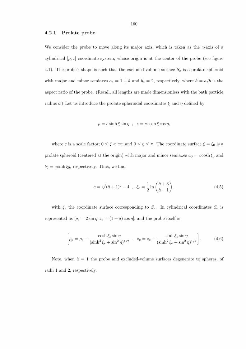
160

4.2.1 Prolate probe

We consider the probe to move along its major axis, which is taken as the z-axis of a

cylindrical [ρ, z] coordinate system, whose origin is at the center of the probe (see figure

4.1). The probe’s shape is such that the excluded-volume surface Se is a prolate spheroid

with major and minor semiaxes ae = 1 + a and be = 2, respectively, where a = a/b is the

aspect ratio of the probe. (Recall, all lengths are made dimensionless with the bath particle

radius b.) Let us introduce the prolate spheroidal coordinates ξ and η defined by

ρ = c sinh ξ sin η , z = c cosh ξ cos η,

where c is a scale factor; 0 ≤ ξ <∞; and 0 ≤ η ≤ π. The coordinate surface ξ = ξ0 is a

prolate spheroid (centered at the origin) with major and minor semiaxes a0 = c cosh ξ0 and

b0 = c sinh ξ0, respectively. Thus, we find

c =√

(a+ 1)2 − 4 , ξe =12

ln(a+ 3a− 1

), (4.5)

with ξe the coordinate surface corresponding to Se. In cylindrical coordinates Se is

represented as [ρe = 2 sin η, ze = (1 + a) cos η], and the probe itself is

[ρp = ρe −

cosh ξe sin η(sinh2 ξe + sin2 η)1/2

, zp = ze −sinh ξe sin η

(sinh2 ξe + sin2 η)1/2

]. (4.6)

Note, when a = 1 the probe and excluded-volume surfaces degenerate to spheres, of

radii 1 and 2, respectively.

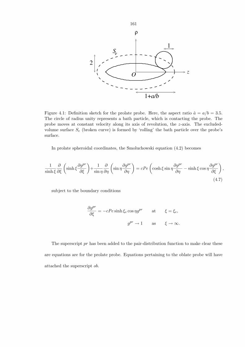
161

Se

1+a/b

ρ

z

1

2

O

Figure 4.1: Definition sketch for the prolate probe. Here, the aspect ratio a = a/b = 3.5.The circle of radius unity represents a bath particle, which is contacting the probe. Theprobe moves at constant velocity along its axis of revolution, the z-axis. The excluded-volume surface Se (broken curve) is formed by ‘rolling’ the bath particle over the probe’ssurface.

In prolate spheroidal coordinates, the Smoluchowski equation (4.2) becomes

1sinh ξ

∂

∂ξ

(sinh ξ

∂gpr

∂ξ

)+

1sin η

∂

∂η

(sin η

∂gpr

∂η

)= cPe

(cosh ξ sin η

∂gpr

∂η− sinh ξ cos η

∂gpr

∂ξ

),

(4.7)

subject to the boundary conditions

∂gpr

∂ξ= −cPe sinh ξe cos ηgpr at ξ = ξe,

gpr → 1 as ξ →∞.

The superscript pr has been added to the pair-distribution function to make clear these

are equations are for the prolate probe. Equations pertaining to the oblate probe will have

attached the superscript ob.

162

O z

ρ

Se

1+a/b

1

2

Figure 4.2: Definition sketch for the oblate probe. Here, the aspect ratio a = a/b = 3.5, andthe legend is the same as in figure 4.1. Again, the probe moves along its axis of revolution(the z-axis) at constant velocity.

4.2.2 Oblate probe

In this case, the probe moves along its minor axis, which is the z-axis of a cylindrical [ρ, z]

coordinate system. The shape of Se is an oblate spheroid, with the same major and minor

semiaxes as in the prolate case (see figure 4.2). We define the oblate spheroidal coordinates

ξ and η by

ρ = c cosh ξ sin η , z = c sinh ξ cos η,

where ξ and η have the same ranges as before; moreover, the scale factor c and the

excluded-volume coordinate surface ξe are again given by (4.5). In fact, one can transform

from prolate to oblate coordinates via the transformation

c→ −ic , cosh ξ → i sinh ξ, (4.8)

where i =√−1 (Morse and Feshbach 1953). Therefore, in the interests of brevity, rather

than state explicitly the excluded-volume shape, probe shape, and Smoluchowski equation

163

in oblate spheroidal coordinates, we note that they can be obtained by applying (4.8) to

the relevant prolate spheroidal equations. Furthermore, in the what follows we perform

detailed calculations for the prolate probe and, wherever possible, employ (4.8) to obtain

results for the equivalent oblate probe.

4.3 Microviscosity

From the pair-distribution function it is possible to calculate many microstructurally-

averaged properties. In the present context, the most interesting is the average external

force on the probe 〈F ext〉, which, as derived by Squires and Brady (2005), is given by

〈F ext〉 = M−1U + nkT

∮ng(r)dSe, (4.9)

whereM = 1/6πηbK is the mobility of the probe, and dSe is the differential area element

of the excluded-volume surface. The mobility factor K accounts for the non-sphericity of

the probe. For the rather complicated probe shape represented by (4.6) evaluation of K is

nontrivial. Therefore, we make the assumption that (for purposes of computing the mobility

only) the probe itself may be approximated as a spheroid with the same major and minor

semiaxes. Thus, the mobility factors are (Happel and Brenner 1965)

Kpr =43(τ2p − 1

)−1/2 [(τ2p + 1) coth−1 τp − τp

]−1, (4.10)

Kob =4a3(λ2

p + 1)−1/2 [

λp − (λ2p − 1) cot−1 λp

]−1,

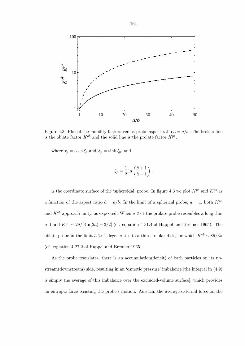
164

1 10 20 30 40 501

10

100

a/b

Kob

Kpr

Figure 4.3: Plot of the mobility factors versus probe aspect ratio a = a/b. The broken lineis the oblate factor Kob and the solid line is the prolate factor Kpr.

where τp = cosh ξp and λp = sinh ξp, and

ξp =12

ln(a+ 1a− 1

),

is the coordinate surface of the ‘spheroidal’ probe. In figure 4.3 we plot Kpr and Kob as

a function of the aspect ratio a = a/b. In the limit of a spherical probe, a = 1, both Kpr

and Kob approach unity, as expected. When a 1 the prolate probe resembles a long thin

rod and Kpr ∼ 2a/[3 ln(2a)− 3/2] (cf. equation 4-31.4 of Happel and Brenner 1965). The

oblate probe in the limit a 1 degenerates to a thin circular disk, for which Kob ∼ 8a/3π

(cf. equation 4-27.2 of Happel and Brenner 1965).

As the probe translates, there is an accumulation(deficit) of bath particles on its up-

stream(downstream) side, resulting in an ‘osmotic pressure’ imbalance [the integral in (4.9)

is simply the average of this imbalance over the excluded-volume surface], which provides

an entropic force resisting the probe’s motion. As such, the average external force on the

165

probe required to maintain its velocity at U is greater than if the probe were traveling in

the absence of bath particles. One can interpret the increase in external force as an incre-

ment to a ‘microviscosity’ of the dispersion: from Stokes drag law, 〈F extz 〉 = 6πηbKUηr (the

external force is, by symmetry, directed solely along the z-axis), a dimensionless relative

microviscosity ηr is defined

ηr = 1 +nkT

6πηbKU

∮nzgdSe,

where nz = n·U . It is natural to define a microviscosity increment, ∆ηr, as

∆ηr =nkT

6πηbKU

∮nzgdSe,

representing the contribution to the microviscosity due to the interaction of the probe

with bath particles. For the prolate probe the increment may be written as

∆ηprr =

6φKprPe

∫ π

0gpr cos η sin ηdη. (4.11)

Recall, φ = 4πnb3/3 is the volume fraction of bath particles. In the oblate case the

increment is

∆ηobr =

3(1 + a)2φ2KobPe

∫ π

0gob cos η sin ηdη. (4.12)

166

4.4 Analytical results

4.4.1 Near equilibrium Pe 1

For small Pe the Brownian diffusion of bath particles dominates over advection by the

moving probe; the microstructure is only slightly perturbed from its equilibrium state.

This is the passive-microrheology, or linear-response, regime in which the microstructural

deformation is proportional to the probe velocity. Therefore, we write the pair-distribution

function as g = 1 + Pef , where f satisfies Laplace’s equation and must vanish at large

distances. In the prolate case the no-flux condition on the excluded-volume surface reads

∂fpr

∂ξ= −c sinh ξe cos η at ξ = ξe,

representing a dipolar forcing. The solution for fpr is found to be

fpr =c(τ2

e − 1)coth−1 τe − τe(τe coth−1 τe − 1)

(τ coth−1 τ − 1) cos η, (4.13)

where τ = cosh ξ and τe = cosh ξe. We note the ‘angular’ dependence of cos η, giving fpr

the structure a diffusive dipole directed along U . From (4.11), the microviscosity increment

is calculated as

∆ηprr =

1Kpr

[8(τ2

e − 1)1/2(τe coth−1 τe − 1)coth−1 τe − τe(τe coth−1 τe − 1)

]φ,

where we have used c(τ2e − 1)1/2 = 2. Using the transformation (4.8) on (4.13), we find

in the oblate case

fob =c(λ2

e + 1)λe(1− λe cot−1 λe)− cot−1 λe

(λ cot−1 λ− 1) cos η,

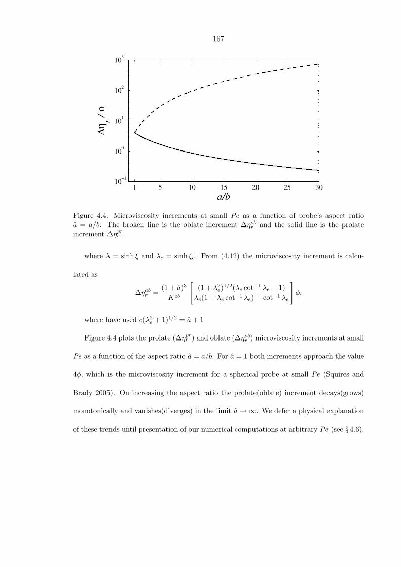
167

1 5 10 15 20 25 3010−1

100

101

102

103

a/b

∆ηr /

φ

Figure 4.4: Microviscosity increments at small Pe as a function of probe’s aspect ratioa = a/b. The broken line is the oblate increment ∆ηob

r and the solid line is the prolateincrement ∆ηpr

r .

where λ = sinh ξ and λe = sinh ξe. From (4.12) the microviscosity increment is calcu-

lated as

∆ηobr =

(1 + a)3

Kob

[(1 + λ2

e)1/2(λe cot−1 λe − 1)

λe(1− λe cot−1 λe)− cot−1 λe

]φ,

where have used c(λ2e + 1)1/2 = a+ 1

Figure 4.4 plots the prolate (∆ηprr ) and oblate (∆ηob

r ) microviscosity increments at small

Pe as a function of the aspect ratio a = a/b. For a = 1 both increments approach the value

4φ, which is the microviscosity increment for a spherical probe at small Pe (Squires and

Brady 2005). On increasing the aspect ratio the prolate(oblate) increment decays(grows)

monotonically and vanishes(diverges) in the limit a→∞. We defer a physical explanation

of these trends until presentation of our numerical computations at arbitrary Pe (see § 4.6).

168

4.4.2 Far from equilibrium Pe 1

For large Pe advection dominates the microstructure, and Brownian diffusion is important

only in a thin boundary layer on the upstream side of the probe. The boundary layer

represents (in a frame fixed on the moving probe) a balance between the strong advection

of bath particles (with velocity −U) towards the probe and diffusion, which enables the bath

particles to pass around the (impenetrable) probe. As a result, there is a large accumulation

of bath particles (g 1) in the boundary layer. Downstream of the probe advection carries

bath particles away: a region of low-particle density (g ≈ 0), or wake, is present. In

this subsection, we present a simple physical argument to calculate the boundary-layer

microstructure. However, note that (as shown in appendix 4.B) the same conclusions may

be obtained from a rigorous asymptotic analysis. In what follows, we examine the oblate

and prolate cases separately.

4.4.2.1 Oblate probe

As mentioned above, the boundary layer signifies a balance between ‘radial’ diffusion (D∇2ξg)

and advection (U⊥·∇ξg) with the perpendicular component of the probe velocity (U⊥ = U·ξ).

Equating these two terms gives an approximate (first order) model for the microstructure

in the boundary layer, which, in dimensional terms, reads

D∂2gob

∂t2+ Uc cosh ξe cos η

∂gob

∂t= 0, (4.14)

where t = ξ − ξe is a dimensionless coordinate perpendicular to the (local) excluded-

volume surface (Se), and c cosh ξe = a+b is the major semiaxis of Se. The solution of (4.14)

169

is

gob ∼ Aob(η)e−U(a+b)t cos η/D. (4.15)

Clearly, this solution is valid only upstream of the probe, 0 ≤ η ≤ π/2; downstream

there is a wake in which g ≈ 0. We integrate across the boundary layer to obtain the local

surface density σ:

σ =∫ ∞

0Aob(η)e−U(a+b)t cos η/Ddt =

DAob(η)U(a+ b) cos η

. (4.16)

At steady state σ must be independent of the angular coordinate η, to ensure there is

no accumulation of bath particles on Se; thus, Aob ∼ cos η. The constant of proportionality

can be determined through a flux balance on the boundary layer. In general, the oblate

shape of the probe leads to a complicated boundary-layer geometry. However, we can make

progress in the limit a b, where Se degenerates to a circular disk of radius a + b and

thickness 4b (see figure 4.5). The flux of bath particles Qin towards the disk is simply

Qin = π(a+ b)2g∞U,

where g∞(= 1) is the far-field value of the pair-distribution function. At steady state,

Qin is balanced by a flux Qout of particles exiting the boundary layer. The bath-particle

surface density σ is advected around Se with the parallel component of velocity U|| = U·η =

−U sinh ξe sin η/(cosh2 ξe − sin2 η)1/2 and finally leaves the boundary layer from the edge

of the disk, over a cylindrical (exit) surface of perimeter 2π(a + b) and thickness 2b. (The

thickness of the disk edge is 4b; however the boundary layer terminates half way along the

edge. Thus, the thickness of the exit surface is 2b.) The edge corresponds to η = 1/2, for

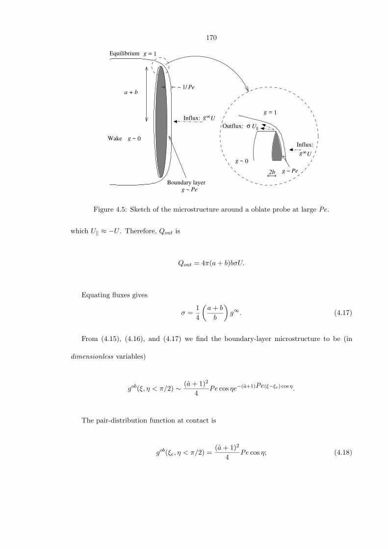
170

2b

U||σ

~ 1/ Pe

8g U

8g U

g = 1

g ~ 0

g = 1

g ~ 0

Boundary layer

Influx:

Influx:

Outflux:

a + b

Wake

Equilibrium

g ~ Pe

g ~ Pe

Figure 4.5: Sketch of the microstructure around a oblate probe at large Pe.

which U|| ≈ −U . Therefore, Qout is

Qout = 4π(a+ b)bσU.

Equating fluxes gives

σ =14

(a+ b

b

)g∞. (4.17)

From (4.15), (4.16), and (4.17) we find the boundary-layer microstructure to be (in

dimensionless variables)

gob(ξ, η < π/2) ∼ (a+ 1)2

4Pe cos ηe−(a+1)Pe(ξ−ξe) cos η.

The pair-distribution function at contact is

gob(ξe, η < π/2) =(a+ 1)2

4Pe cos η; (4.18)

171

thus, there is a large O(Pe = Ub/D) excess of bath particles in front of the probe.

Moreover, this excess is amplified by a geometrical factor of (a+ 1)2/4. Properly, though,

for the circular disk (and, actually, for all oblate probes) one should scale lengths with the

disk radius a+ b (it being the dominant length scale in the problem), which yields

gob(ξe, η < π/2) =(a+ 1)

4Pea cos η,

where Pea = U(a+ b)/D is a Peclet number based on the major semiaxis of Se, rather

than the bath particle radius b. Now we find the O(Pea) build-up of bath particles is

amplified by (a + 1)/4, which is simply the ratio of the surface areas for entry [π(a + b)2]

and exit [4πb(a + b)] of bath particles: physically, bath particles are advected into the

boundary layer through a much [O(a+ b)] larger area (the disk face) than from which they

can escape (the disk edge), leading to large amplification of the O(Pe) build-up.

Finally, from (4.12) and (4.18) (i.e., with the Peclet number based on the bath particle

radius) the microviscosity increment is

∆ηobr =

3(1 + a)2φ2KobPe

∫ π/2

0gob cos η sin ηdη =

(a+ 1)4

8φ

Kob.

4.4.2.2 Prolate probe

For the prolate probe at large Pe an equation for the boundary-layer microstructure may

be obtained by balancing again ‘radial’ diffusion (D∇2ξg) and advection (U⊥ ·∇ξg), viz.

D∂2gpr

∂t2+ Uc sinh ξe cos η

∂gpr

∂t= 0, (4.19)

where t = ξ−ξe, and c sinh ξe = 2b is the minor semiaxis of the excluded-volume surface.

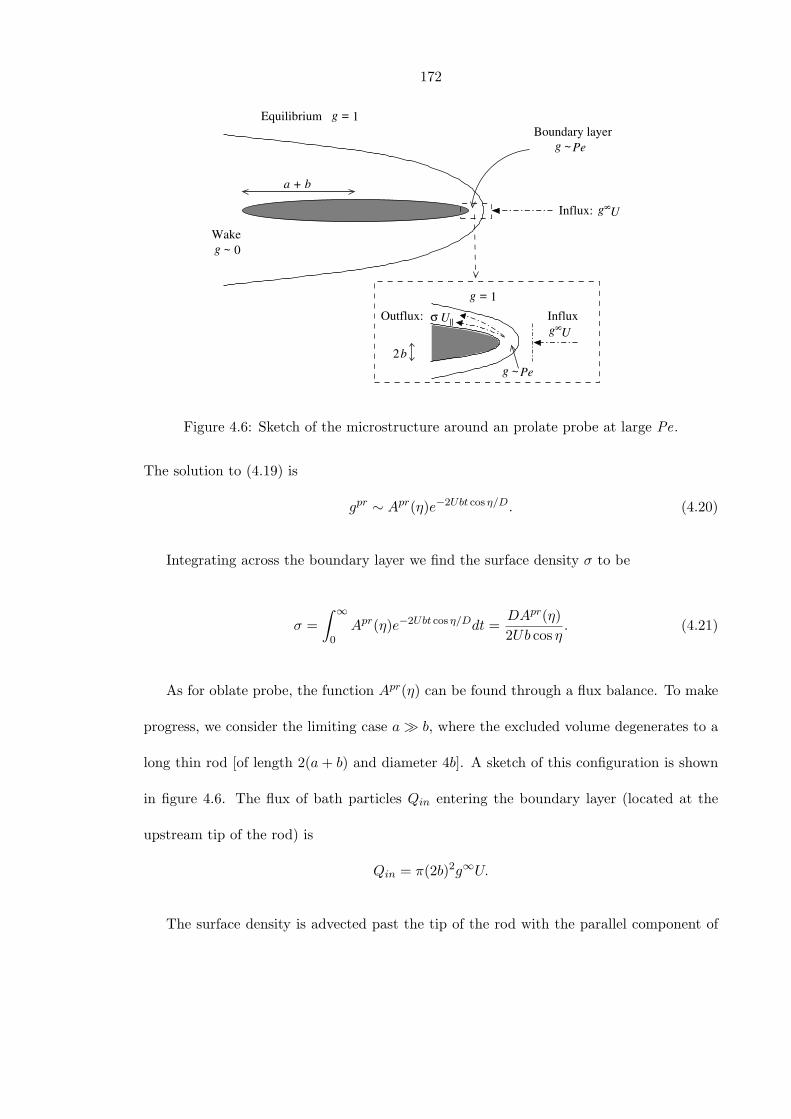
172

g 8U

g 8U

2b

U||

g = 1

g = 1

Pe

Pe

Equilibrium

Wake

a + b

Boundary layer

Influx

Influx:

Outflux: σ

g ~ 0

g ~

g ~

Figure 4.6: Sketch of the microstructure around an prolate probe at large Pe.

The solution to (4.19) is

gpr ∼ Apr(η)e−2Ubt cos η/D. (4.20)

Integrating across the boundary layer we find the surface density σ to be

σ =∫ ∞

0Apr(η)e−2Ubt cos η/Ddt =

DApr(η)2Ub cos η

. (4.21)

As for oblate probe, the function Apr(η) can be found through a flux balance. To make

progress, we consider the limiting case a b, where the excluded volume degenerates to a

long thin rod [of length 2(a+ b) and diameter 4b]. A sketch of this configuration is shown

in figure 4.6. The flux of bath particles Qin entering the boundary layer (located at the

upstream tip of the rod) is

Qin = π(2b)2g∞U.

The surface density is advected past the tip of the rod with the parallel component of

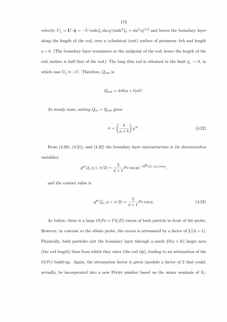
173

velocity U|| = U ·η = −U cosh ξe sin η/(sinh2 ξe + sin2 η)1/2 and leaves the boundary layer

along the length of the rod, over a cylindrical (exit) surface of perimeter 4πb and length

a+ b. (The boundary layer terminates at the midpoint of the rod; hence the length of the

exit surface is half that of the rod.) The long thin rod is obtained in the limit ξe → 0, in

which case U|| ≈ −U . Therefore, Qout is

Qout = 4πb(a+ b)σU.

At steady state, setting Qin = Qout gives

σ =(

b

a+ b

)g∞. (4.22)

From (4.20), (4.21), and (4.22) the boundary layer microstructure is (in dimensionless

variables)

gpr(ξ, η < π/2) ∼ 2a+ 1

Pe cos ηe−2Pe(ξ−ξe) cos η,

and the contact value is

gpr(ξe, η < π/2) =2

a+ 1Pe cos η. (4.23)

As before, there is a large O(Pe = Ub/D) excess of bath particle in front of the probe.

However, in contrast to the oblate probe, the excess is attenuated by a factor of 2/(a+ 1).

Physically, bath particles exit the boundary layer through a much [O(a + b)] larger area

(the rod length) than from which they enter (the rod tip), leading to an attenuation of the

O(Pe) build-up. Again, the attenuation factor is given (modulo a factor of 2 that could,

actually, be incorporated into a new Peclet number based on the minor semiaxis of Se:

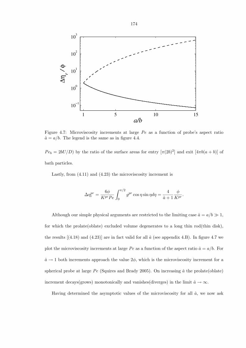
174

1 5 10 15

10−1

100

101

102

103

a/b

∆ηr /

φ

Figure 4.7: Microviscosity increments at large Pe as a function of probe’s aspect ratioa = a/b. The legend is the same as in figure 4.4.

Peb = 2bU/D) by the ratio of the surface areas for entry [π(2b)2] and exit [4πb(a + b)] of

bath particles.

Lastly, from (4.11) and (4.23) the microviscosity increment is

∆ηprr =

6φKprPe

∫ π/2

0gpr cos η sin ηdη =

4a+ 1

φ

Kpr.

Although our simple physical arguments are restricted to the limiting case a = a/b 1,

for which the prolate(oblate) excluded volume degenerates to a long thin rod(thin disk),

the results [(4.18) and (4.23)] are in fact valid for all a (see appendix 4.B). In figure 4.7 we

plot the microviscosity increments at large Pe as a function of the aspect ratio a = a/b. For

a → 1 both increments approach the value 2φ, which is the microviscosity increment for a

spherical probe at large Pe (Squires and Brady 2005). On increasing a the prolate(oblate)

increment decays(grows) monotonically and vanishes(diverges) in the limit a→∞.

Having determined the asymptotic values of the microviscosity for all a, we now ask

175

1 2 3 4 5 6 7 8 9 10−5

−4

−3

−2

−1

0

1

2

3

a/b

[ ∆η r(P

e <<1

) −∆η

r(Pe >

>1) ]

/ φ

Figure 4.8: Difference in microviscosity increments at small Pe and large Pe as a functionof probe aspect ratio a = a/b. The broken(solid) line is the difference in the oblate(prolate)increment

how it transitions between these limits. To this end, it is useful to to examine the difference

between the microviscosity in the limits Pe 1 and Pe 1 (see figure 4.8). For the

prolate probe the microviscosity (for a fixed a) at small Pe is greater than at large Pe, which

suggests the microviscosity decreases, or ‘velocity-thins’, as a function of Pe. However, the

situation is not so simple for the oblate probe. On increasing a (above unity) the difference

between small Pe and large Pe microviscosities is positive and growing, indicating that

the microviscosity velocity-thins. This trend continues until a = 1.89 (to two decimal

places), at which point the difference reaches a maximum value and proceeds to decreases

monotonically with increasing a. The difference in microviscosities is zero for a = 3.52

(to two decimal places), and for higher a it becomes increasingly negative. This behavior

is rather unexpected and suggests that the microviscosity increment for the oblate probe

increases, or ‘velocity-thickens’, as a function of Pe for a > 3.52. The conclusions of our

asymptotic analysis will be verified by results from numerical solution of the Smoluchowski

176

equation and a physical explanation for this unexpected behavior will be offered. Next, we

describe the methods used to perform the numerical computations.

4.5 Numerical methods

In the preceding section, we calculated the microstructure and microviscosity increments

for small and large departures from equilibrium, using analytical perturbation methods.

Here, we present numerical methods that facilitate computation of the microstructure and

microviscosity at arbitrary Pe. One should note, however, that the Smoluchowski equation

does in fact admit an exact solution in spheroidal coordinates (see appendix 4.A for details).

Therefore, one could, in principle, use the exact solution to develop analytical formulas for

the microviscosity valid for all Pe. The exact solution is found by separation of variables

and takes the usual form of a eigenfunction summation; unfortunately, the complexity of

the eigenfunctions coupled with the mixed (Robin) no-flux boundary condition (4.4) on Se,

makes numerical evaluation of the exact solution computationally prohibitive (especially at

large Pe, where one needs to retain a large number of eigenfunctions). Therefore, we choose

to solve the Smoluchowski equation numerically, using two different methods.

For Pe < 10 an expansion of the pair-distribution function in a series of Legendre poly-

nomials is employed. This approach was used previously in determining the microstructure

around a externally forced spherical probe (Khair and Brady 2006). As Pe increases one

requires more terms in the expansion to faithfully represent the increasingly complex mi-

crostructure, which is computationally taxing. Therefore, for Pe > 10 we solve the Smolu-

chowski equation using a finite-difference scheme, which accurately captures the boundary

layer and wake structure present at large Pe. The two methods are described next.

177

4.5.1 Legendre polynomial expansion

For for the prolate probe, the pair-distribution gpr function is written as

gpr(ξ, η) = 1 +∞∑

n=0

fprn (ξ)Pn(cos η), (4.24)

where Pn(z) is the Legendre polynomial of degree n and argument z. This expansion is

substituted into the Smoluchowski equation (4.7) and, after using the orthogonality property

of the Legendre polynomials on the interval [0, π], we arrive at a coupled set of ordinary

differential equations for the expansion coefficients fprn (ξ):

1sinh ξ

(sinh ξ

∂fprn

∂ξ

)− n(n+ 1)fpr

n = −cPe (αn cosh ξ + βn sinh ξ) , (4.25)

where the advective coupling terms are

αn =(n+ 1)(n+ 2)

2n+ 3fpr

n+1 +n(1− n)2n− 1

fprn−1,

βn =n+ 12n+ 3

∂fprn+1

∂ξ+

n

2n− 1∂fpr

n−1

∂ξ.

The boundary conditions on the expansion coefficients are

∂fprn

∂ξ= −c sinh ξe Pe

(δn1 +

n+ 12n+ 3

fprn+1 +

n

2n− 1fpr

n−1

)at ξ = ξe, (4.26)

fprn → 0 as ξ →∞, (4.27)

where δij is Kronecker’s delta. The system of equations is solved using the Matlab

boundary-value problem solver bvp4c. The summation in (4.24) is truncated at n = nmax;

for a given value of Pe, the choice of nmax is made be requiring the resulting microviscosity

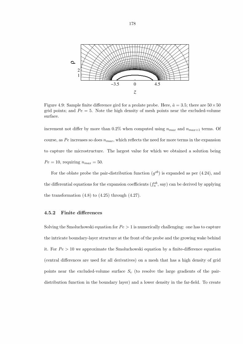
178

0−3.5 4.5

12

z

ρ

Figure 4.9: Sample finite difference gird for a prolate probe. Here, a = 3.5; there are 50×50grid points; and Pe = 5. Note the high density of mesh points near the excluded-volumesurface.

increment not differ by more than 0.2% when computed using nmax and nmax+1 terms. Of

course, as Pe increases so does nmax, which reflects the need for more terms in the expansion

to capture the microstructure. The largest value for which we obtained a solution being

Pe = 10, requiring nmax = 50.

For the oblate probe the pair-distribution function (gob) is expanded as per (4.24), and

the differential equations for the expansion coefficients (fobn , say) can be derived by applying

the transformation (4.8) to (4.25) through (4.27).

4.5.2 Finite differences

Solving the Smoluchowski equation for Pe > 1 is numerically challenging: one has to capture

the intricate boundary-layer structure at the front of the probe and the growing wake behind

it. For Pe > 10 we approximate the Smoluchowski equation by a finite-difference equation

(central differences are used for all derivatives) on a mesh that has a high density of grid

points near the excluded-volume surface Se (to resolve the large gradients of the pair-

distribution function in the boundary layer) and a lower density in the far-field. To create

179

this non-uniform mesh in (physical) ξ-space we employ a mapping from the semi-infinite

domain ξ ∈ [ξe,∞) to the finite interval p ∈ [0, 1], viz.

ln p = −y(ω +

1− ω

1 + y

),

where ω is a parameter and y = Pe(ξ − ξe). Using a uniform grid in p-space one can

(via adjustment of ω) place a large number of nodes near ξ = ξe, to accurately model the

near-field microstructure (e.g., see figure 4.9).

The linear system of equations resulting from discretization of the Smoluchowski equa-

tion is solved using a simple Jacobi iteration (the method closely resembles that of Khair

and Brady 2006, who calculated the microstructure around a spherical probe at large Pe).

As Pe increases, one requires are greater number of grid points for the method to converge:

the maximum value of Pe for which a solution was obtained being Pe = 100.

4.6 Results

In this section, we present results for the microstructure and microviscosity at arbitrary Pe

for different values of a. In figure 4.10 the microstructural deformation, g − 1, is plotted

in the symmetry plane of a prolate probe of aspect ratio a = 3.5, as a function of Pe. For

Pe 1 diffusion dominates: the deformation is approximately for-aft symmetric about

the probe, with an O(Pe) accumulation(depletion) on its upstream(downstream) side, in

agreement with the linear-response analysis of § 4.4.1. Moving to Pe ∼ O(1) advection

comes into play, and the symmetry is broken. For larger Pe the probe acts as a ‘bulldozer’:

it accumulates bath particles in a O(Pe−1) thin boundary-layer on its upstream side and

leaves a wake of bath-particle free suspending fluid behind it. Note, the ‘width’ of the

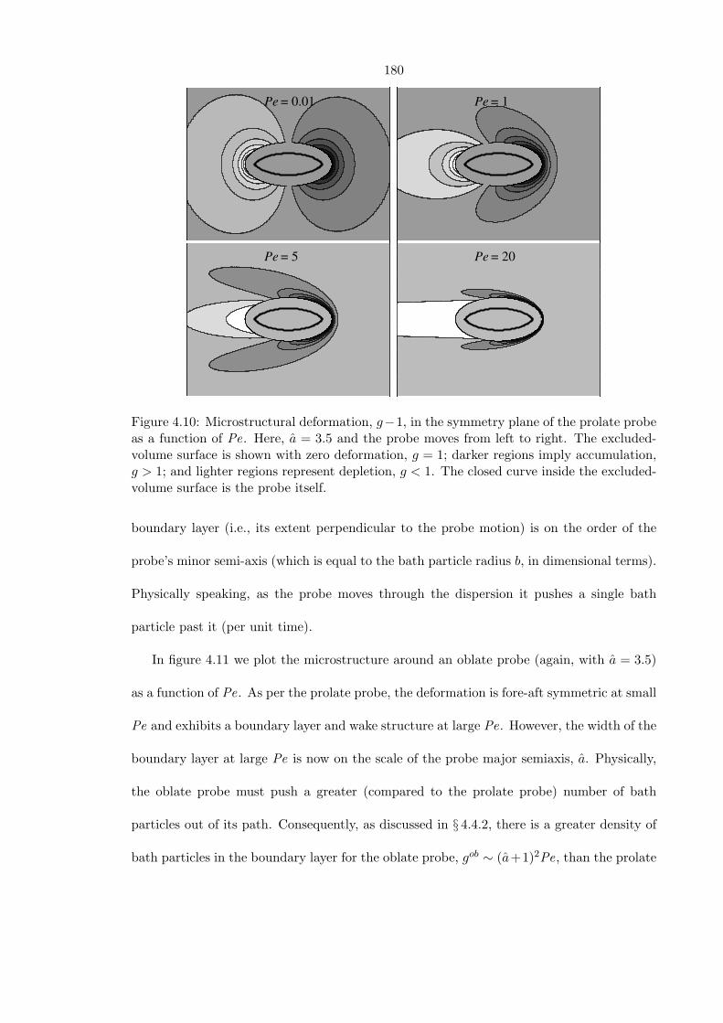
180

Pe = 0.01 Pe = 1

Pe = 5 Pe = 20

Figure 4.10: Microstructural deformation, g−1, in the symmetry plane of the prolate probeas a function of Pe. Here, a = 3.5 and the probe moves from left to right. The excluded-volume surface is shown with zero deformation, g = 1; darker regions imply accumulation,g > 1; and lighter regions represent depletion, g < 1. The closed curve inside the excluded-volume surface is the probe itself.

boundary layer (i.e., its extent perpendicular to the probe motion) is on the order of the

probe’s minor semi-axis (which is equal to the bath particle radius b, in dimensional terms).

Physically speaking, as the probe moves through the dispersion it pushes a single bath

particle past it (per unit time).

In figure 4.11 we plot the microstructure around an oblate probe (again, with a = 3.5)

as a function of Pe. As per the prolate probe, the deformation is fore-aft symmetric at small

Pe and exhibits a boundary layer and wake structure at large Pe. However, the width of the

boundary layer at large Pe is now on the scale of the probe major semiaxis, a. Physically,

the oblate probe must push a greater (compared to the prolate probe) number of bath

particles out of its path. Consequently, as discussed in § 4.4.2, there is a greater density of

bath particles in the boundary layer for the oblate probe, gob ∼ (a+1)2Pe, than the prolate

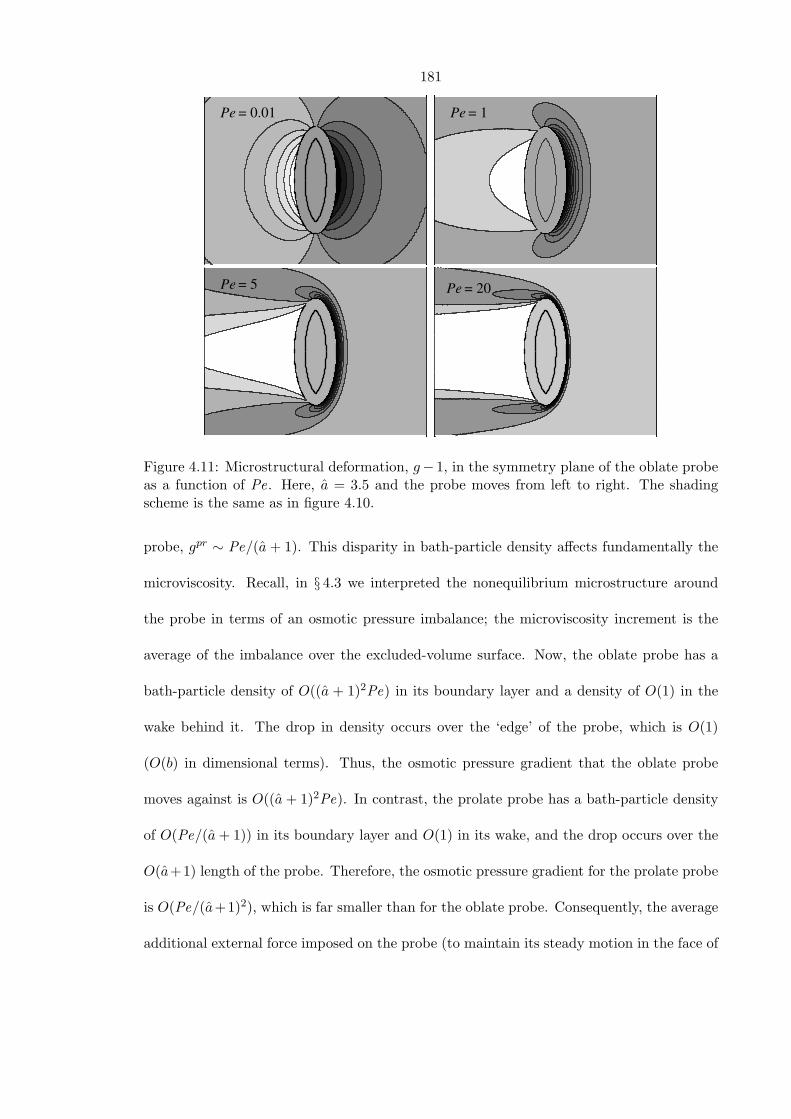
181

Pe = 1Pe = 0.01

Pe = 5 Pe = 20

Figure 4.11: Microstructural deformation, g− 1, in the symmetry plane of the oblate probeas a function of Pe. Here, a = 3.5 and the probe moves from left to right. The shadingscheme is the same as in figure 4.10.

probe, gpr ∼ Pe/(a + 1). This disparity in bath-particle density affects fundamentally the

microviscosity. Recall, in § 4.3 we interpreted the nonequilibrium microstructure around

the probe in terms of an osmotic pressure imbalance; the microviscosity increment is the

average of the imbalance over the excluded-volume surface. Now, the oblate probe has a

bath-particle density of O((a + 1)2Pe) in its boundary layer and a density of O(1) in the

wake behind it. The drop in density occurs over the ‘edge’ of the probe, which is O(1)

(O(b) in dimensional terms). Thus, the osmotic pressure gradient that the oblate probe

moves against is O((a+ 1)2Pe). In contrast, the prolate probe has a bath-particle density

of O(Pe/(a+ 1)) in its boundary layer and O(1) in its wake, and the drop occurs over the

O(a+1) length of the probe. Therefore, the osmotic pressure gradient for the prolate probe

is O(Pe/(a+1)2), which is far smaller than for the oblate probe. Consequently, the average

additional external force imposed on the probe (to maintain its steady motion in the face of

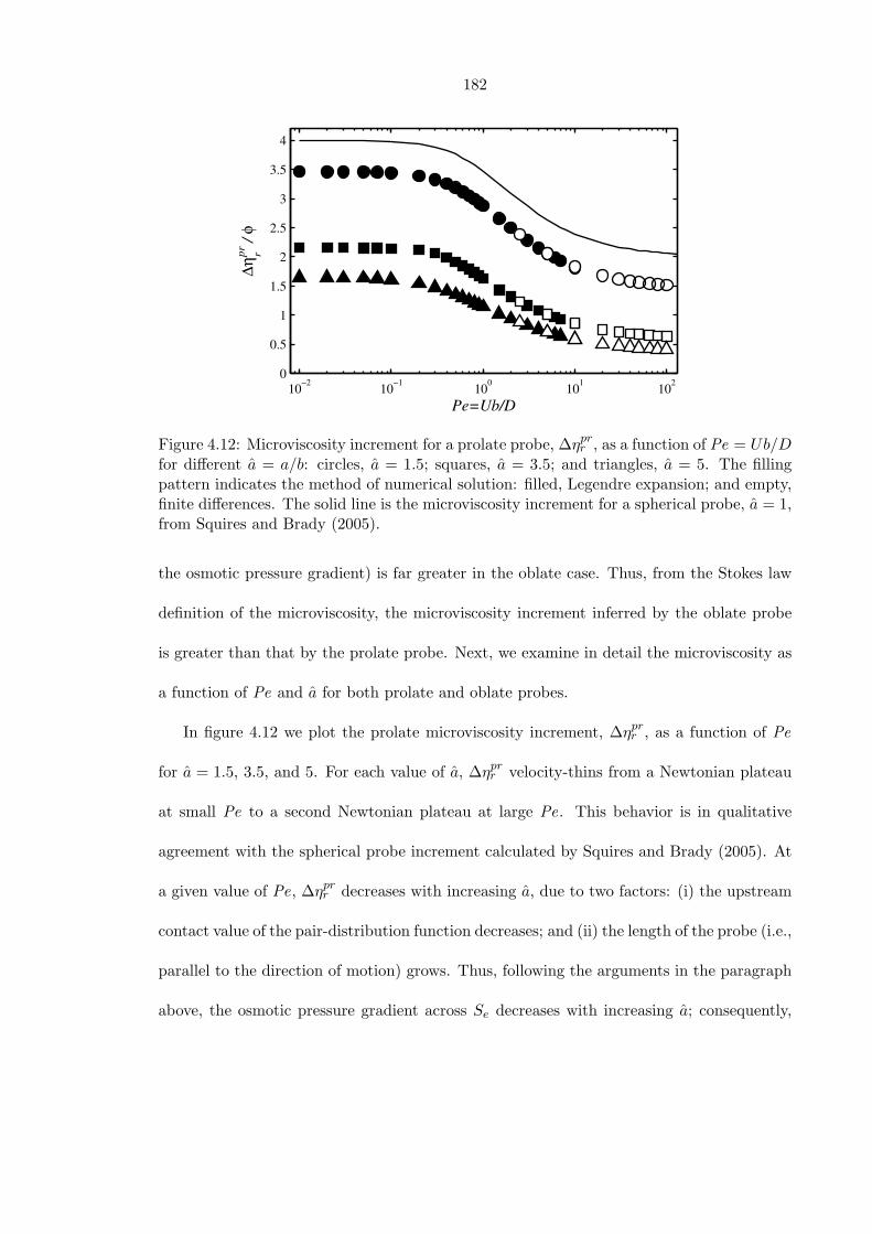
182

10−2 10−1 100 101 1020

0.5

1

1.5

2

2.5

3

3.5

4

Pe=Ub/D

∆ηrpr

/ φ

Figure 4.12: Microviscosity increment for a prolate probe, ∆ηprr , as a function of Pe = Ub/D

for different a = a/b: circles, a = 1.5; squares, a = 3.5; and triangles, a = 5. The fillingpattern indicates the method of numerical solution: filled, Legendre expansion; and empty,finite differences. The solid line is the microviscosity increment for a spherical probe, a = 1,from Squires and Brady (2005).

the osmotic pressure gradient) is far greater in the oblate case. Thus, from the Stokes law

definition of the microviscosity, the microviscosity increment inferred by the oblate probe

is greater than that by the prolate probe. Next, we examine in detail the microviscosity as

a function of Pe and a for both prolate and oblate probes.

In figure 4.12 we plot the prolate microviscosity increment, ∆ηprr , as a function of Pe

for a = 1.5, 3.5, and 5. For each value of a, ∆ηprr velocity-thins from a Newtonian plateau

at small Pe to a second Newtonian plateau at large Pe. This behavior is in qualitative

agreement with the spherical probe increment calculated by Squires and Brady (2005). At

a given value of Pe, ∆ηprr decreases with increasing a, due to two factors: (i) the upstream

contact value of the pair-distribution function decreases; and (ii) the length of the probe (i.e.,

parallel to the direction of motion) grows. Thus, following the arguments in the paragraph

above, the osmotic pressure gradient across Se decreases with increasing a; consequently,

183

10−2 10−1 100 101 1020

5

10

15

20

25

30

35

40

Pe=Ub/D

∆ηrob

/ φ

Figure 4.13: Microviscosity increment for an oblate probe, ∆ηobr , as a function of Pe = Ub/D

for different a = a/b. The legend is the same as in figure 4.12.

the additional external force, and hence the microviscosity, also decrease. Ultimately, as

a→∞ — a long thin rod probe — the microviscosity vanishes for all Pe. In this limit, the

rod appears infinitely long on the scale of a bath particle; as such, the bath particles cannot

‘see’ the ends of the rod, and the microstructure is not disturbed by the moving rod.

Figure 4.13 plots the microviscosity increment for the oblate probe, ∆ηobr , versus Pe for

a = 1.5, 3.5, and 5. We note for a given value of Pe that ∆ηobr increases with increasing a,

which can be explained by the following argument. As a increases the area of the excluded-

volume surface upon which bath particles from upstream are incident grows (∼ a2). This

leads to an increase in the contact value of the pair-distribution function on the upstream

side of the probe. Moreover, unlike the prolate probe, as a increases the extent of the probe

parallel to its motion (i.e., its thickness) stays fixed at 2 (2b in dimensional terms). Thus, the

osmotic pressure gradient of bath particles across Se increases with increasing a. As a result,

the average external force on the probe, and hence the microviscosity, increase. Finally, as

a → ∞ — a thin circular disk probe — the microviscosity diverges for all Pe: essentially,

184

the probe must overcome an infinite osmotic pressure gradient to maintain steady motion.

The behavior of the oblate increment for a given value of a as a function of Pe is far

more complicated than the prolate increment. For a = 1.5, in analogy to the spherical

and prolate probe microviscosities, the oblate increment monotonically velocity-thins from

a small Pe plateau (∆ηobr /φ = 5.80 at Pe = 0.001) to a plateau at high Pe (∆ηob

r /φ =

3.55 at Pe = 100). However, for a = 3.5 the increment is approximately independent

of Pe: it undergoes a small amount of velocity-thinning initially (from ∆ηobr /φ = 16.87

at Pe = 0.001), which is recovered by velocity-thickening at Pe ∼ O(1) and greater (at

Pe = 100 we find ∆ηobr /φ = 16.81). For a = 5 the increment monotonically velocity-

thickens from a small Pe plateau (∆ηobr /φ = 29.13 at Pe = 0.001) until a plateau at large

Pe is reached (∆ηobr /φ = 37.46 at Pe = 100). Note, these numerical results are in agreement

entirely with the asymptotic analysis presented in § 4.4. (In fact, a = 3.5 was chosen for

numerical calculations because it is close the value, a = 3.52, at which the small and large

Pe microviscosities are predicted to be equal, cf. figure 4.8.)

At first glance, the transition of ∆ηobr from velocity-thinning to -thickening with increas-

ing a might seem somewhat strange. There is a relatively simple explanation, however. Let

us define the microstructural deformation F ob = gob − 1. Recall, from (4.12) the mi-

croviscosity increment is directly proportional to F ob averaged over the excluded-volume

surface, Se. At small Pe the deformation is forced by the no-flux condition at contact

[dF ob/dξ = −(a+1)Pe cos η at ξ = ξe], and the contact value of the deformation was found

to be (see § 4.4.1)

F ob(Pe 1) = (a+ 1)H(λe)Pe cos η,

185

where

H(λe) =(1 + λ2

e)1/2(λe cot−1 λe − 1)

λe(1− λe cot−1 λe)− cot−1 λe.

The function H(λe) = 0.5 for a = 1, and H(λe) → 0.64 (to two decimal places) as

a → ∞. Hence, to make progress we assume H(λe) ≈ 0.5 for all a. The microstructural

deformation averaged over Se is

〈F ob(Pe 1)〉Se =∫ π

0F ob(Pe 1) cos η sin ηdη = 2(a+ 1)H(λe)Pe ≈ (a+ 1)Pe.

At large Pe, from the boundary-layer analysis in § 4.4.2 we found

F ob(Pe 1) =14(a+ 1)2Pe cos η;

importantly, this solution is valid only upstream of the probe, η ≤ π/2; downstream

there is wake in which gob ≈ 0. The surface-averaged deformation is

〈F ob(Pe 1)〉Se =∫ π/2

0F ob(Pe 1) cos η sin ηdη =

14(a+ 1)2Pe.

The small- and large-Pe averaged deformations are equal, (〈F ob(Pe 1)〉Se = 〈F ob(Pe

1)〉Se), at a = 3, which is close to the transition point a = 3.52 of ∆ηobr from velocity-thinning

to -thickening. (Of course, using the full form of H(λe) would yield the correct value of

a = 3.52 from our simple analysis.)

Before proceeding to the next section, we pause to make a comment about the micro-

viscosity increment ∆ηr as a function of Pe. As mentioned above, ∆ηr is proportional to

the contact value of the pair-distribution function, which is O(Pe) for all Pe. And, since

there is a factor of 1/Pe multiplying the microstructural integrals in (4.11) and (4.12),

186

∆ηr ∼ O(Pe0) for all Pe. (The microstructural pictures at small and large Pe are, of

course, very different: for Pe 1 the probe causes a small O(Pe) deformation over a

large O(1/Pe) region; in the singular limit of Pe → ∞ there is a large O(Pe) deforma-

tion in a small O(1/Pe) thin boundary layer.) However, while we know ∆ηr is of O(Pe0)

at both small and large Pe, there is no way (without detailed calculation) of knowing in

which limit it is greater (and hence if ∆ηr thins or thickens with increasing Pe). The thin-

ning/thickening behavior is dependent on the detailed geometry — in our case the (prolate

or oblate) probe shape and a — of the probe and bath particle configuration. This points

up the care that must be taken when selecting a probe (in terms of its shape, size, and

orientation) for use in a particular active microrheology experiment.

4.7 Discussion

In this study, we have developed a model for active (nonlinear) microrheology experiments

using non-spherical probe particles. We consider the probe to be a body of revolution moving

along its symmetry axis at constant velocity, through a colloidal dispersion of spherical bath

particles. The probe’s shape is such that the excluded-volume, or contact, surface between

it and a bath particle is a(n) prolate(oblate) spheroid when its major(minor) axis is the

axis of revolution. The average external force imposed on the probe (to maintain its steady

motion) can be interpreted in terms of a microviscosity of the dispersion via application of

Stokes drag law. This is, possibly, the simplest model system one could conceive; however,

as shown in the preceding sections, the resulting microrheology is nontrivial.

It is instructive to determine to what extent the results from a particular microrhe-

ological experiment represent the true, or macrorheological, properties of a material. As

mentioned in § 4.1, for highly complex or unknown materials it is, in general, not possible

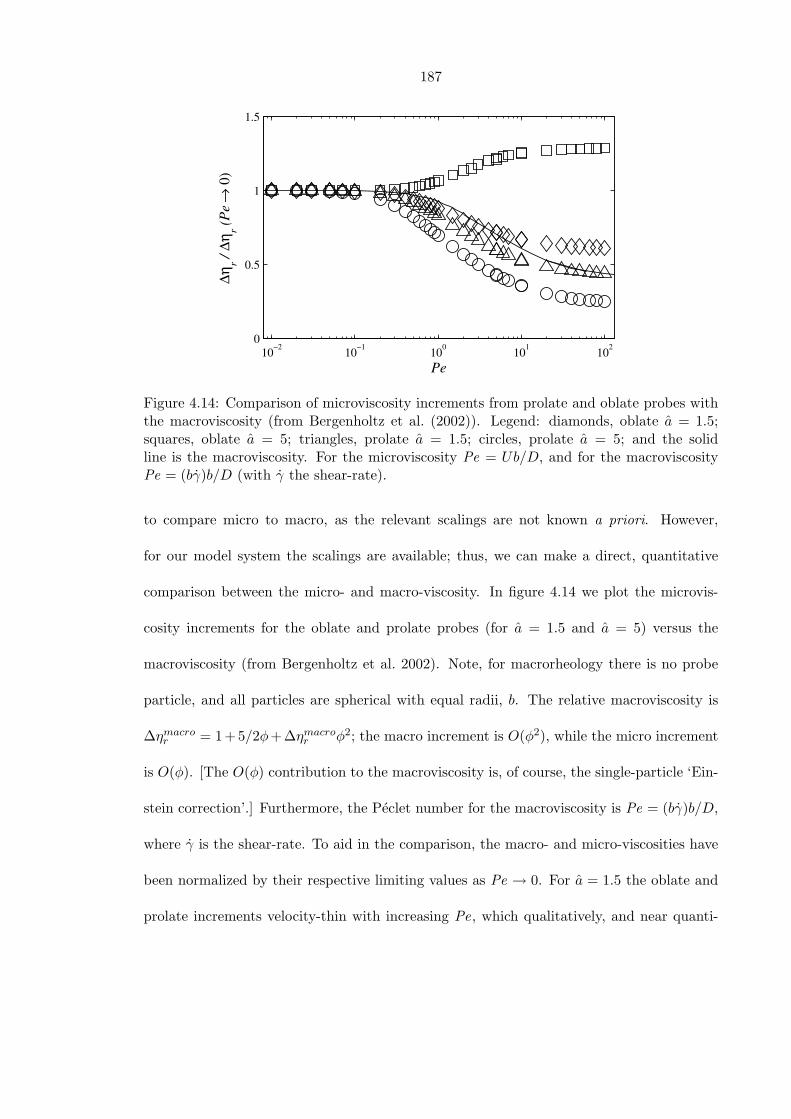
187

10−2 10−1 100 101 1020

0.5

1

1.5

Pe

∆ηr /

∆ηr (P

e → 0

)

Figure 4.14: Comparison of microviscosity increments from prolate and oblate probes withthe macroviscosity (from Bergenholtz et al. (2002)). Legend: diamonds, oblate a = 1.5;squares, oblate a = 5; triangles, prolate a = 1.5; circles, prolate a = 5; and the solidline is the macroviscosity. For the microviscosity Pe = Ub/D, and for the macroviscosityPe = (bγ)b/D (with γ the shear-rate).

to compare micro to macro, as the relevant scalings are not known a priori. However,

for our model system the scalings are available; thus, we can make a direct, quantitative

comparison between the micro- and macro-viscosity. In figure 4.14 we plot the microvis-

cosity increments for the oblate and prolate probes (for a = 1.5 and a = 5) versus the

macroviscosity (from Bergenholtz et al. 2002). Note, for macrorheology there is no probe

particle, and all particles are spherical with equal radii, b. The relative macroviscosity is

∆ηmacror = 1+5/2φ+∆ηmacro

r φ2; the macro increment is O(φ2), while the micro increment

is O(φ). [The O(φ) contribution to the macroviscosity is, of course, the single-particle ‘Ein-

stein correction’.] Furthermore, the Peclet number for the macroviscosity is Pe = (bγ)b/D,

where γ is the shear-rate. To aid in the comparison, the macro- and micro-viscosities have

been normalized by their respective limiting values as Pe → 0. For a = 1.5 the oblate and

prolate increments velocity-thin with increasing Pe, which qualitatively, and near quanti-

188

tatively, mimics the ‘shear-thinning’ of the macroviscosity. However, for a = 5.0 the oblate

increment velocity-thickens for all Pe, which is qualitatively different from the macrovis-

cosity behavior. One should not think, though, this disagreement somehow invalidates the

microrheological results. On the contrary, it simply highlights the fundamental physical

differences between microrheology and macrorheology (for detailed discussions of these dif-

ferences see Squires and Brady 2005; Khair and Brady 2006), and emphasizes the care

that must be taken when comparing the results from a microrheology experiment using

non-spherical probes to the ‘equivalent’ macrorheological measurements.

The theoretical framework presented in this work can be used to study other related

problems. A natural extension is to consider a non-spherical (oblate or prolate) probe that

is translating with fixed velocity at an angle (β, say) to its symmetry axis (see figure 4.15).

In this sense, the present study considers the special case β = 0, in which the microstructure

is axisymmetric about the direction of motion; however, for non-zero β the microstructure

is now fully three dimensional. Consequently, to maintain steady motion not only must

an additional external force (above the Stokes drag) be imposed on the probe, but also

an external torque to prevent the probe from rotating. In appendix 4.C we present a

preliminary analysis of this problem for small and large Pe. In the linear-response regime

(Pe 1) the symmetry of the O(Pe) microstructural deformation (4.C-2) dictates that

the dispersion does not exert a torque on the probe. In contrast, far from equilibrium

(Pe 1) the highly nonlinear microstructure does necessitate the application an external

torque. Importantly, we find that the external torque is directed perpendicular to the plane

of motion; therefore, there is no tendency for the probe to rotate out of that plane or about

its symmetry axis. Furthermore, for longwise, β = 0, and broadside, β = π/2, motion the

external torque vanishes, indicating that both are steady modes of translation. However,

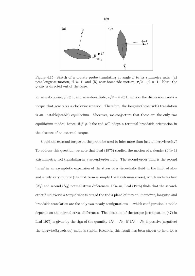
189

z

Ux

z

β

U

x

β

(a) (b)

Figure 4.15: Sketch of a prolate probe translating at angle β to its symmetry axis: (a)near-longwise motion, β 1; and (b) near-broadside motion, π/2 − β 1. Note, they-axis is directed out of the page.

for near-longwise, β 1, and near-broadside, π/2− β 1, motion the dispersion exerts a

torque that generates a clockwise rotation. Therefore, the longwise(broadside) translation

is an unstable(stable) equilibrium. Moreover, we conjecture that these are the only two

equilibrium modes; hence, if β 6= 0 the rod will adopt a terminal broadside orientation in

the absence of an external torque.

Could the external torque on the probe be used to infer more than just a microviscosity?

To address this question, we note that Leal (1975) studied the motion of a slender (a 1)

axisymmetric rod translating in a second-order fluid. The second-order fluid is the second

‘term’ in an asymptotic expansion of the stress of a viscoelastic fluid in the limit of slow

and slowly varying flow (the first term is simply the Newtonian stress), which includes first

(N1) and second (N2) normal stress differences. Like us, Leal (1975) finds that the second-

order fluid exerts a torque that is out of the rod’s plane of motion; moreover, longwise and

broadside translation are the only two steady configurations — which configuration is stable

depends on the normal stress differences. The direction of the torque [see equation (47) in

Leal 1975] is given by the sign of the quantity 4N1 +N2: if 4N1 +N2 is positive(negative)

the longwise(broadside) mode is stable. Recently, this result has been shown to hold for a

190

prolate spheroid of arbitrary a for the special case N1 = −2N2 (Galdi 2000).

Our analysis for a prolate probe gave a stable broadside orientation which, assuming

that the second-order fluid model is applicable to the hard-sphere colloidal dispersion, sug-

gests that 4N1 +N2 < 0 at large Pe. Is this consistent with macrorheological observations?

To answer this question, we note that the microstructure at large Pe was found via a simple

‘radial-balance approximation’ of the full boundary-layer equations (see appendix 4.C for

details), used originally by Brady and Morris (1997) in calculation of the microstructure of

a sheared dispersion at large Pe. From the radial-balance microstructure Brady and Morris

(1997) computed the normal stress differences of the dispersion, finding that N1 ≡ 0 (by

the symmetry properties of the approximate boundary-layer equations) and N2 < 0 at large

Pe. This implies that 4N1 +N2 is indeed negative, in agreement with our microrheological

findings that broadside translation is stable. However, note that Bergenholtz et al. (2002)

solved numerically the full macrorheological boundary-layer equations and found N1 to be

‘small’ and positive at large Pe; infact their results give 4N1 +N2 > 0, which suggests that

the longwise translation should be stable. Clearly, one needs to solve the full microrhe-

ological boundary-layer equations (4.C-3) to determine if the broadside mode is stable as

a result of the radial-balance approximation (i.e., would a solution of the full equations

give a stable longwise translation). Furthermore, as shown by Zarraga et al. (2000), for

non-colloidal dispersions (Pe−1 ≡ 0) both N1 and N2 are proportional to the shear-rate γ,

whereas for the second-order fluid N1 and N2 scale as γ2. Thus, it is not clear that one

can use Leal’s (Leal 1975) results to infer normal stress differences from a prolate probe

translating at large Pe.2 Nevertheless, the discussion above has shown that microrheology2However, colloidal dispersions near equilibrium (Pe 1) posses normal stress differences, N1 and N2,

that do scale as γ2 (Brady and Vicic 1995), in accordance with the second-order fluid model. Thus one canuse Leal’s analysis to infer normal stress differences for a prolate probe moving at small Pe. Of course, Pemust be sufficient in magnitude such that the dispersion is out of the linear-response regime, for which thereis no torque on the probe.

191

with non-spherical probes has the potential to give information on normal stress differences.

In this study we supposed, for simplicity, that the minor semiaxis of the probe was equal

in size to the bath particle radius. This allowed the probe-bath geometry to be specified by a

single quantity: the probe aspect ratio a = a/b. One could, however, relax this assumption

by setting the bath particle radius equal to c (here, c is not to be confused with the scale

factor in spheroidal coordinates, of course). Now, the geometry is set by the ratios a1 = a/b

and a2 = a/c. The additional degree of freedom allows us to study several interesting

limiting cases: for example, (i) a1 1 and a2 ∼ O(1) — a flat disk (oblate) / thin rod

(prolate) translating past bath particles of comparable size; and (ii) a1 1 and a2 1 —

a flat disk (oblate) / thin rod (prolate) moving through a dispersion of much larger bath

particles. Case (i) is particularly interesting, as while the oblate probe is a flat disk, it

now pushes only one bath particle out of its path (per unit time). Hence, one expects the

microviscosity inferred from it may not velocity-thicken at large Pe.

Recently, Khair and Brady (2005) examined a spherical probe executing small-amplitude

oscillations in a colloidal dispersion. The small-amplitude condition requires that the Peclet

number be much less than unity; the system is in the linear-response (passive) regime.

There is, however, no such restriction on the (appropriately non-dimensionalized) oscillation

frequency (α, say). In this limit, the microstructural deformation has a component that is in

phase with the probe oscillation and a component that is out of phase. Through application

of Stokes drag law one can define a complex microviscosity of the dispersion — the real and

imaginary parts of which correspond to liquid-like and solid-like response, respectively.

In that sense, the oscillating probe may be used to study the ‘microviscoelasticity’ of the

dispersion As a variation on that (and the present) theme, one may consider a non-spherical

probe moving parallel to its axis of revolution with a small-amplitude oscillatory velocity.

192

Again, the microstructural response will contain in-phase and out of phase components, from

which a complex microviscosity can be inferred. For a spherical probe Khair and Brady

(2005) demonstrated that the Cox-Merz rule is obeyed to a reasonable degree (see figure

4 in that paper). Recall, the Cox-Merz rule states that the frequency dependence of the

modulus of the complex microviscosity should be almost identical to the Pe dependence of

the steady microviscosity. For the oblate probe, it would be interesting to see if the complex

microviscosity ‘frequency-thickens’ at large α, in analogy to the velocity-thickening of the

nonlinear (steady) microviscosity at large Pe for a > 3.5 (see figure 4.13). If the complex

microviscosity does not thicken this would constitute a violation of the Cox-Merz rule.

193

4.8 Bibliography

M. Atakhorammi, G. H. Koenderink, C. F. Schmidt, and F. C. MacKintosh. Short-time

inertial response of viscoelastic fluids: observation of vortex propagation. Phys. Rev.

Lett., 95:208302, 2005.

J. Bergenholtz, J. F. Brady, and M. Vicic. The non-Newtonian rheology of dilute colloidal

suspensions. J. Fluid Mech., 456:239–275, 2002.

J. F. Brady and J. F. Morris. Microstructure of strongly sheared suspensions and its impact

on rheology and diffusion. J. Fluid Mech., 348:103–139, 1997.

J. F. Brady and M. Vicic. Normal stresses in colloidal dispersions. J. Rheol., 39:545–566,

1995.

B. R. Daniels, B. C. Masi, and D. Wirtz. Probing single-cell micromechanics in vivo: the

micorheology of C. elegans developing embryos. Biophys. J., 90:4712–4719, 2006.

C. Flammer. Spheroidal wave functions. Stanford University Press, 1957.

G. P. Galdi. Slow steady fall of rigid bodies in a second-order fluid. J. Non-Newtonian

Fluid Mech., 90:81–89, 2000.

F. Gittes, B. Schnurr, P. D. Olmsted, F. C. MacKintosh, and C. F. Schimdt. Microscopic

viscoelasticity: shear moduli of soft materials determined from thermal fluctuations. Phys.

Rev. Lett., 79:3286–3289, 1997.

P. Habdas, D. Schaar, A. C. Levitt, and E. R. Weeks. Forced motion of a probe particle

near the colloidal glass transition. Europhys. Lett., 79:477–483, 2004.

J. Happel and H. Brenner. Low Reynolds number Hydrodynamics. Prentice-Hall, 1965.

194

L. Joly, C. Ybert, and L. Bocquet. Probing the nanohydrodynamics at the liquid-solid

interfaces using thermal motion. Phys. Rev. Lett., 96:046101, 2006.

A. S. Khair and J. F. Brady. “Microviscoelasticity” of colloidal dispersions. J. Rheol., 49:

1449–1481, 2005.

A. S. Khair and J. F. Brady. Single particle motion in colloidal dispersions: A simple model

for active and nonlinear microrheology. J. Fluid Mech., 557:73–117, 2006.

L. G. Leal. The slow motion of a slender rod-like particle in a second-order fluid. J. Fluid

Mech., 69:305–337, 1975.

F. C. MacKintosh and C. F. Schmidt. Microrheology. Curr. Opin. Colloid Interface Sci.,

4:300–307, 1999.

R. E. Mahaffy, C. K. Shih, F. C. MacKintosh, and J. Kas. Scanning probe-based frequency

dependent microrheology of polymer gels and biological cells. Phys. Rev. Lett., 85:880–

883, 2000.

T. G. Mason, K. Ganesan, J. H. van Zanten, D. Wirtz, and S. C. Kuo. Particle tracking

microrheology of complex fluids. Phys. Rev. Lett., 79:3282–3285, 1997.

T. G. Mason and D. A. Weitz. Optical measurements of frequency-dependent linear vis-

coelastic moduli of complex fluids. Phys. Rev. Lett., 74:1250–1253, 1995.

A. Meyer, A. Marshall, B. G. Bush, and E. M. Furst. Laser tweezer microrheology of a

colloidal suspension. J. Rheol., 50:77–92, 2006.

P. M. Morse and H. Feshbach. Methods of theoretical physics. Part II. McGraw-Hill, 1953.

195

I. S. Sohn and R. Rajagopalan. Microrheology of model quasi-hard-sphere dispersions. J.

Rheol., 48:117–140, 2004.

T. M. Squires and J. F. Brady. A simple paradigm for active and nonlinear microrheology.

Phys. Fluids, 17:073101, 2005.

N. Ter-Oganessian, D. A. Pink, and A. Boulbitch. Active microrheology of networks com-

posed of semiflexible polymers: theory and comparison with simulations. Phys. Rev. E.,

72:041511, 2005a.

N. Ter-Oganessian, B. Quinn, D. A. Pink, and A. Boulbitch. Active microrheology of

networks composed of semiflexible polymers: computer simulation of magnetic tweezers.

Phys. Rev. E, 72:041510, 2005b.

R. S. Tu and V. Breedveld. Microrheological detection of protein unfolding. Phys. Rev. E.,

72:041914, 2005.

T. A. Waigh. Microrheology of complex fluids. Rep. Prog. Phys., 68:685–742, 2005.

H. H. Wensink and H. Lowen. Rhythmic cluster generation in strongly driven colloidal

dispersions. Phys. Rev. Lett., 97:038303, 2006.

I. E. Zarraga, D. A. Hill, and D. T. Leighton. The characterization of the total stress

of concentrated suspensions of noncolloidal spheres in Newtonian fluids. J. Rheol., 44:

185–220, 2000.

196

Appendices to chapter 4

197

4.A Exact solution of the Smoluchowski equation

Here, we derive an exact solution to the Smoluchowski equation (4.2) in spheroidal coordi-

nates. In the interests of brevity, we deal with the prolate probe only; however, it is possible

to calculate an exact solution for the oblate probe also (either from first principles or by

simply using the transformation (4.8) in the formulas below).

First, we write the pair-distribution function as

gpr = 1 + fpre−cκ cosh ξ cos η,

where κ = Pe/2. Substituting this into the Smoluchowski equation (4.7) we find that

fpr satisfies a modified Helmholtz equation:

1sinh ξ

∂

∂ξ

(sinh ξ

∂fpr

∂ξ

)+

1sin η

∂

∂η

(sin η

∂fpr

∂η

)= c2κ2(sinh2 ξ + sin2 η)fpr, (4.A-1)

subject to the boundary conditions

∂fpr

∂ξ= −2κ cos η

[1 + 2e(a+1)κ cos η

]at ξ = ξe,

fpr → 0 as ξ →∞.

The solution to (4.A-1) is found by separation of variables (see, e.g., Flammer 1957)

and can be written as an eigenfunction expansion:

fpr =∞∑

n=0

AnS0n(ik, µ)R(3)0n (ik, τ),

where µ = cos η, τ = cosh ξ, k = cκ, and the An are expansion coefficients. The function

198

S0n is the (axisymmetric) angle function of the first kind and is defined as a sum of Legendre

polynomials:

S0n(ik, µ) =∞∑

r=0,1

d0nr (ik)Pr(µ),

where the summation is over even(odd) values of r when n is even(odd). The summation

coefficients d0nr obey a recurrence relation — see equation 3.1.4 of Flammer (1957). The

function R(3)0n is known as the radial function of third kind, which vanishes for large τ (thus

satisfying the far-field boundary condition). Formally, R(3)0n may be written as a summation

of spherical Hankel functions of the first kind (denoted as h(1)r )

R(3)0n (ik, τ) =

∞∑r=0,1

d0nr (ik)

−1∞∑

r=0,1

ir−nd0nr (ik)h(1)

r (ikτ).

To satisfy the boundary condition at contact we require

∞∑n=0

An∂R

(3)0n

∂ξ|ξeS0n(ik, µ) = −2κµ

[1 + 2e(a+1)κµ

].

We note that the angle functions satisfy are orthogonal on the interval [−1, 1]:

∫ 1

−1S0n(ik, µ)S0p(ik, µ)dµ = δnpN0n(k);

the normalization constantN0n(k) is given by equation 3.1.33 of Flammer (1957). Hence,

the constants An are given by

An = − 2κ

N0k∂R

(3)0n

∂ξ |ξe

[∫ 1

−1S0n(ik, µ)µdµ+ 2

∫ 1

−1S0n(ik, µ)e(a+1)κµµdµ

]. (4.A-2)

The first integral in (4.A-2) can be performed analytically; however, the second integral

199

must be computed numerically, which does, unfortunately, limit the usefulness of the exact

solution.

Finally, from (4.11) the microviscosity increment is given by

∆ηpr =6φ

KprPe

∞∑n=0

AnR(3)0n (ik, τe)

∫ 1

−1S0n(ik, µ)e−(a+1)κµµdµ.

Again, this integral must be performed numerically.

4.B Asymptotic analysis at large Pe

In this appendix, we present a rigorous asymptotic analysis of the microstructure at large Pe,

to confirm the findings of our simple physical arguments in § 4.4.2. Detailed calculations

are performed for the prolate probe, and the results for the equivalent oblate probe are

obtained via the transformation (4.8).

At large Pe advection dominates the microstructure and, except near the probe, the

Smoluchowski equation (4.2) reduces to U ·∇g = 0, implying g is constant along a ‘stream-

line’. The far-field condition (4.3) dictates this constant to be unity; however, this solution

does not satisfy the no-flux boundary condition on the excluded-volume surface Se (4.4).

The Smoluchowski equation is in fact singular in the limit Pe−1 → 0, and there exists

an ‘inner’ region (or boundary layer) adjacent to the probe in which Brownian diffusion

balances advection, thus enabling the no-flux condition on Se to be met.

To focus on the boundary layer we introduce the stretched, or inner, coordinate y =

200

Pe(ξ − ξe). The Smoluchowski equation in prolate spheroidal coordinates (4.7) becomes

Pe2

sinh ξe + Pe−1y cosh ξe

∂

∂y

[(sinh ξe + Pe−1y cosh ξe)

∂gpr

∂y

]+

1sin η

∂

∂η

(sin η

∂gpr

∂η

)= cPe

[(cosh ξe + Pe−1y sinh ξe) sin η

∂gpr

∂η− Pe

(sinh ξe + Pe−1y cosh ξe

)cos η

∂gpr

∂y

],

(4.B-1)

subject to the boundary conditions

∂gpr

∂y= −c sinh ξe cos ηgpr at y = 0.

gpr → 1 as y →∞,

Inside the boundary layer we expand the pair-distribution function as gpr(y, η;Pe) =

gpr1 (y, η)Pe + gpr

2 (y, η)+O(Pe−1). Inserting this expansion into (4.B-1) yields equations for

gpr1 and gpr

2 . For gpr1 we have

∂2gpr1

∂y2+ c sinh ξe cos η

∂gpr1

∂y= 0,

∂gpr1

∂y+ c sinh ξe cos ηgpr

1 = 0 at y = 0,

gpr1 → 0 as y →∞,

which has the solution

gpr1 (y, η) = A(η)e−cy sinh ξe cos η.

The ‘angular’ function A(η) will be found at the next order. Note, this solution is

only valid upstream of the probe (0 ≤ η ≤ π/2), where advection balances diffusion in the

201

boundary layer. Downstream of the probe, π/2 ≤ η ≤ π, bath particles are advected away

and there exists a wake in which g ≈ 0.

The system for gpr2 reads

∂2gpr2

∂y2+ c sinh ξe cos η

∂gpr2

∂y= c cosh ξe

(sin η

∂gpr1

∂η− y cos η

∂gpr1

∂y

)− coth ξe

∂gpr1

∂y,

∂gpr2

∂y+ c sinh ξe cos ηgpr

2 = 0 at y = 0.

gpr2 → 1 as y →∞,

The far-field condition on gpr2 ensures correct matching to the advective outer solution

of unity. Some straightforward working yields

gpr2 (y, η) = [β1(η) + β2(η)y + β3(η)y2]e−cy sinh ξe cos η − β2

c sinh ξe cos η,

where

β1(η) = − coth ξec sinh ξe

[A(η)cos3 η

+tan ηcos η

dA(η)dη

]− B(η)c sinh ξe cos η

,

β2(η) = − coth ξe

[tan η

dA(η)dη

+ (1 + sec2 η)A(η)],

β3(η) = −c cosh ξe2 cos η

A(η).

One can determine the function B(η) by continuing the perturbation expansion to the

next order in Pe; this is not, however, required for our current purposes. To satisfy the

far-field condition on gpr2 requires β2(η) = −c sinh ξe cos η, from which we obtain an equation

for A(η):

tan ηdA(η)dη

+ (1 + sec2 η)A(η) = c sinh ξe tanh ξe cos η,

202

which has the solution A(η) = 12c sinh ξe tanh ξe cos η. Hence, the pair-distribution func-

tion in the boundary layer may be written as

gpr(y, η;Pe) =12c sinh ξe tanh ξe cos ηe−cPe(ξ−ξe) sinh ξe cos η +O(1). (4.B-2)

From (4.11) we find that at large Pe the microviscosity increment is

∆ηprr =

6φKprPe

∫ π/2

0gpr cos η sin ηdη =

4a+ 1

φ

Kpr+O(Pe−1),

where we have used the relations c sinh ξe = 2 and tanh ξe = 2/(a+ 1)

For the oblate probe, using the transformation (4.8) on (4.B-2), we find the pair-

distribution function in the boundary layer is

gob(y, η;Pe) =12c cosh ξe coth ξe cos ηe−cPe(ξ−ξe) cosh ξe cos η +O(1),

and from (4.12) the microviscosity increment is

∆ηobr =

3(1 + a)2φ2KobPe

∫ π/2

0gob cos η sin ηdη =

(a+ 1)4

8φ

Kob+O(1).

where we have used c cosh ξe = a+ 1 and coth ξe = (a+ 1)/2. Note, both results above

are in complete agreement with the simple geometric balance presented in § 4.4.2.

203

4.C Prolate probe translating at an angle to its symmetry

axis

Here, we present an asymptotic analysis for a prolate probe translating at an angle β to its

symmetry axis (see figure 4.15). The dimensionless velocity of the probe is

U = cosβz + sinβx.

In addition to an external force 〈F ext〉 (4.9) one must, in general, apply an external

torque 〈T ext〉 to maintain steady motion. The ‘osmotic force’ exerted by the bath particles

on an infinitesimal area dSe of the probe is −nkTg(r)ndSe. Therefore, the average external

torque about the center of the probe is

〈T ext〉 = nkT

∮r ∧ ng(r)dSe,

which for the prolate probe reduces to

〈T ext〉6ηb2U

=6φ

Pe sinh2 ξe

∫ 2π

0

∫ π

0gpr(r)(cos θy − sin θx) sin2 η cos ηdηdθ. (4.C-1)

Here, θ is the azimuthal coordinate about the z-axis. In the linear-response regime

(Pe 1) we write gpr = 1 + Pefpr, where fpr solves Laplace’s equation and vanishes at

large distances. The no-flux condition on the excluded volume surface is

∂fpr

∂ξ= −c (cosβ sinh ξe cos η + sinβ cosh ξe sin η cos θ) at ξ = ξe,

representing a weighted combination of axisymmetric (along z-axis) and

204

non-axisymmetric (along x-axis) forcing. The solution for fpr is found to be

fpr = − 2dQ0

1(τ)/dξ|ξe

cosβ cos ηQ01(τ)−

a+ 1dQ1

1(τ)/dξ|ξe

sinβ sin ηQ11(τ) cos θ, (4.C-2)

where τ = cosh ξ and Qmn (τ) is an associated Legendre polynomial of the second kind.

Using (4.C-2) with (4.C-1) we find that the external torque is identically zero — as a conse-

quence of the symmetry of microstructure — in the linear-response regime. On increasing

Pe this fore-aft symmetry will be broken, resulting in a non-zero torque.

We now consider the opposite extreme, Pe 1, where advection dominates the mi-

crostructure. As in appendix 4.B, the problem is singular in this limit with a boundary

layer adjacent to the probe in which diffusion balances advection. Thus, near Se we stretch

ξ as y = Pe(ξ − ξe). The Smoluchowski equation for gpr in stretched coordinates reads

∂2gpr

∂y2+ Pe−1 coth ξe

∂gpr

∂y= Pe−1c sinβ

sinh2 ξe + sin2 η

sinh ξe sin ηsin θ

∂gpr

∂θ

− c cosβ[(sinh ξe + Pe−1y cosh ξe) cos η

∂gpr

∂y− Pe−1 cosh ξe sin η

∂gpr

∂η

]− c sinβ

[(cosh ξe + Pe−1y sinh ξe) sin η

∂gpr

∂y+ Pe−1 sinh ξe cos η

∂gpr

∂η

]+O(Pe−2);

(4.C-3)

furthermore, gpr must satisfy the boundary conditions

∂gpr

∂y= −c (cosβ sinh ξe cos η + sinβ cosh ξe sin η cos θ) gpr at y = 0, (4.C-4)

gpr → 1 as y →∞. (4.C-5)

One can, in principle, solve for gpr by posing the expansion gpr = Pegpr1 +gpr

2 +O(Pe−1)

as per appendix 4.B; however, the resulting algebra is rather cumbersome. Instead, to find

205

gpr we invoke the ‘radial-balance approximation’ used by Brady and Morris (1997) for the

microstructure of a sheared suspension at large Pe. The physical idea is that the competition

between ‘radial’ advection and diffusion generates the large gradients of gpr present in the

boundary layer. Thus, we form a ‘leading-order’ equation by retaining the O(Pe0) and the

O(Pe−1) radial (∂/∂y) terms in (4.C-3), which gives

∂2gpr

∂y2+ vy

(1 +

1vy

Pe−1 coth ξe + Pe−1∂ ln vy

∂ξey

)∂gpr

∂y= 0, (4.C-6)

where vy is the ‘radial’ advective velocity in the boundary layer:

vy(η, θ) = c (cosβ sinh ξe cos η + sinβ cosh ξe sin η cos θ) . (4.C-7)

The solution to (4.C-6) satisfying (4.C-4) and (4.C-5) is

gpr(y) =1− vy

∫ y0 e

−s(z)dz

1− vy

∫∞0 e−s(z)dz

,

where s(z) is given by

s(z) = vy

[(1 +

1vy

Pe−1 coth ξe

)z +

12Pe−1∂ ln vy

∂ξez2

].

Note, this solution is valid only if vy > 0: the locus of points on the excluded-volume

surface satisfying vy = 0 defines the transition between upstream (vy > 0) and downstream

(vy < 0) regions. Physically, bath particles are advected from upstream towards the probe,

resulting in a boundary layer, while downstream they are advected away from it, giving a

206

low-density wake in which gpr ≈ 0. We can rewrite gpr as

gpr(y) = gpr(0)[1− vy

∫ y

0e−s(z)dz

],

and in the limit Pe →∞ it is found that

gpr(0) = Pe tanh ξevy,

=2Pe

(a+ 1)[2 cosβ cos η + (a+ 1) sinβ sin η cos θ] , (4.C-8)

showing that there is an O(Pe) accumulation of bath particles in the upstream boundary

layer. Note that for β = 0 we recover, modulo a factor of 2, the contact value for a probe

translating along its symmetry axis, cf. (4.23).

Substituting the above into (4.C-1) we can now evaluate the external torque. However,

there is a subtlety: the range of η in (4.C-1) is formally between 0 to π (from the upstream to

downstream end of the probe), while the contact value (4.C-8) is valid only in the upstream

region, from η = 0 to η = ηl, where vy(ηl, θ) = 0. (The interval η < ηl < π corresponds to

the downstream region in which gpr ≈ 0.) From (4.C-7), ηl satisfies the equation

2 cosβ cos ηl + (a+ 1) sinβ sin ηl cos θ = 0. (4.C-9)

To make progress, we focus on the limits of near-longwise (β 1) and near-broadside

(π/2− β 1) translation. For β 1, the solution to (4.C-9) is

ηl =π

2+a+ 1

2β cos θ,

207

i.e., the O(β) tilting causes the boundary layer-wake transition to occur slightly down-

stream of the probe midpoint (η = π/2). The external torque for β 1 is found to be

〈T ext〉6πηb2U

= 3φβ

[(a+ 1

2

)2

− 1

]y, (4.C-10)

where we have used sinh2 ξe = [(a+ 1)2/4− 1]−1. Similarly, for π/2− β 1 we have

ηl = π − a+ 12

(π2− β

)cos θ;

thus, in near-broadside translation the boundary layer occupies nearly the entire upstream-

facing side of the probe, and the resulting torque is

〈T ext〉6πηb2U

=158φ(π

2− β

)4(a+ 1

2

)4[(

a+ 12

)2

− 1

]y. (4.C-11)

From (4.C-10) and (4.C-11) one can make the following observations. First, for a spher-

ical probe, a = 1, the torque vanishes as expected. Second, the torque is directed along

the positive y-axis; hence, there is no tendency for the probe to rotate out of its plane of

motion (or about its symmetry axis). Third, for longwise, β = 0, and broadside, β = π/2,

motion the torque vanishes, indicating that both of these are possible equilibrium modes

of translation. However, by referring to figure 4.15 for near-longwise and near-broadside

motion the external torque rotates the probe anticlockwise; consequently, the dispersion

exerts a torque that generates a clockwise rotation. Hence, in the absence of an external

torque the longwise(broadside) translation is an unstable(stable) equilibrium configuration.

Furthermore, we conjecture that these are the only two equilibrium modes; hence, if β 6= 0

the rod will adopt a terminal broadside orientation.

208

Finally, we note that in obtaining (4.C-8) the O(Pe−1) ‘angular’ terms in (4.C-3) were

neglected, while the O(Pe−1) ‘radial’ terms were retained, thus forming a ‘radial balance’

with the leading order [O(Pe0)] terms (4.C-6). This is generally not a valid procedure, as

the angular terms in (4.C-3) will affect the O(Pe0) angular structure of the pair-distribution

function at contact, gpr(0). However, to leading order [O(Pe)] the angular structure of the

contact value should not be affected by the neglect of the O(Pe−1) angular terms, although

the magnitude of gpr(0) might be. [Indeed, this is evident for β = 0, where the radial-

balance solution (4.C-8) gives a contact value that is identical, modulo a factor of 2, to the

solution of the full boundary-layer equations, (4.23).] Therefore, while a solution of the full

boundary-layer equations (4.C-3) may well alter the magnitude of the torque in (4.C-10)

and (4.C-11), we do not expect the sense of rotation to change.

209

Chapter 5

On the motion of two particlestranslating with equal velocitiesthrough a colloidal dispersion

210

5.1 Introduction

Colloidal dispersions, comprising (sub-) micrometer sized particles in a suspending fluid,

occur in a variety of natural and man-made settings: inks, aerosols, foodstuffs, paints, and

biological materials are but a few everyday examples. From an academic viewpoint, the

length and time scales relevant to colloidal dispersions place them in a perhaps unique

position at the intersection of fluid dynamics, statistical mechanics, and macromolecular

chemistry. A central goal of colloid science is the calculation of the macroscopic, or ef-

fective, properties of a dispersion (e.g., diffusion coefficients, viscosity, conductivity), from

interactions at the microscopic level, or microscale. In these materials, it is the inter-

play of hydrodynamic, interparticle, and Brownian (or thermal) forces that determines the

microscale configuration, or microstructure, of the colloidal particles. In equilibrium the

balance is between interparticle and Brownian forces, and the microstructure is given by the

familiar Boltzmann distribution. The action of external agents, such as ambient flow-fields

or body forces, drives the microstructure out of equilibrium, where hydrodynamic forces

now enter the description.

In this work, we study the nonequilibrium microstructure created by two colloidal

(‘probe’) particles translating with equal, fixed velocities through an otherwise undisturbed

colloidal dispersion. The driven motion of the probes pushes the dispersion’s microstructure

out of equilibrium; counteracting this is the Brownian diffusion of the colloidal ‘bath’ parti-

cles, which acts to heal this microstructural wound. As a consequence of the microstructural

deformation, the dispersion exerts an entropic, or thermal, force on each of the probes, which

is a function of the separation between the probes d, and the dimensionless velocity of the

probes, or Peclet number, Pe. Our aim is to calculate the entropic forces on the probes over

211

the entire range of d and Pe, for which one must, of course, determine the nonequilibrium

microstructure.

In equilibrium, it is well known that entropic forces between colloidal particles are often

produced by the addition of macromolecular entities to the suspending fluid. These entities

may be other (usually smaller) colloidal particles (Crocker et al. 1999), polymers (Verma

et al. 1998), or stiff rods (Heldon et al. 2003). The generated forces have important physical

consequences and applications, including crystallization (Anderson and Lekkerkerker 2002)

and self-assembly (Yodh et al. 2001). A classic example, first noted by Asakura and Oosawa

(1958), is the so-called ‘depletion attraction’, where two colloidal particles in a dilute bath

of smaller colloids experience an attractive (depletion) force when the excluded-volume

surfaces of the large particles overlap, owing to an increase in volume available to the bath

particles. The depletion force can lead to depletion flocculation (Jenkins and Snowden 1996)

and has been seen to promote phase separation in binary colloid mixtures (Kaplan et al.

1994). The diluteness of bath particles is crucial; for more concentrated systems interactions

between the bath particles themselves can lead to a repulsive force between the two large

colloids (Crocker et al. 1999; Tehver et al. 1999).

Away from equilibrium, the depletion interaction between colloidal particles must com-

pete with external driving mechanisms. This can lead to pattern formation on macroscopic

(i.e., much greater the particle size) length scales: e.g., ‘lane’ formation in binary mixtures

of oppositely driven colloids (Dzubiella et al. 2002; Chakrabarti et al. 2004). To our knowl-

edge, the only theoretical study of depletion forces out of equilibrium is that of Dzubiella

et al. (2003), who computed the forces on two fixed colloidal particles in a drifting bath

of smaller Brownian particles. As expected, for non-zero drift velocities the forces on the

fixed particles are not equal, which Dzubiella et al. (2003) interpreted as a violation of

212

Newton’s third law. Their analytical approach [Brownian Dynamics (BD) simulations were

also performed] consisted of superimposing the microstructural deformations induced by a

single fixed particle in the drifting bath, at the (two) locations relevant to the two-particle

configuration. This is valid only if the fixed particles are widely separated and the (appro-

priately non-dimensionalized) drift velocity is small; somewhat surprisingly, the theoretical

results are in good agreement with the BD simulations even when these two conditions are

not met. In this work, subject to the assumptions listed below, we are able to avoid such

approximations and restrictions in computing the microstructural deformation caused by

the moving probes.

In the present study, we make four important assumptions. First, for simplicity, we take

the probes and bath particles to be spherical and of equal size. However, note that the

theory developed in § 5.2 for the nonequilibrium microstructure may be easily extended to

different-sized probe and bath particles. Hence, we could, if desired, recover the small bath

particle limit of Dzubiella et al. (2003). Second, in analogy to classic theories of depletion

forces in equilibrium, we take the volume fraction of bath particles to be small, so that in-

teractions between bath particles may be neglected. Furthermore, to facilitate an analytical

treatment, we assume the microstructure is determined by interactions of the probes with

a single bath particle. Third, hydrodynamic interactions mediated by the suspending fluid

are neglected. While seemingly over-restrictive, this condition can be realized for particles

whose excluded-volume (or hard-sphere) radii are much greater than their physical (or hy-

drodynamic) radii, such as present in sterically- or charge-stabilized dispersions. Fourth, we

assume that the particles move along their line of centers, d. Therefore, the microstructural

deformation is axisymmetric about d, and the (entropic) forces on the probes are directed

along d. With these conditions in place, we are able to derive a closed equation for the

213

nonequilibrium microstructure in terms of a ‘conditional pair-distribution function’, which

gives the probability of finding a bath particle at a particular location, given the two-probe

configuration.

The rest of the chapter is organized as follows. In § 5.2.1 we present the three-body

Smoluchowski equation governing the spatio-temporal evolution of the nonequilibrium mi-

crostructure, and the entropic forces on the probes are derived in § 5.2.2. The Smoluchowski

equation must be solved numerically and, as discussed in § 5.3, different approaches are used

for overlapping and non-overlapping probe excluded-volumes. Results are presented in § 5.4

and concluding remarks offered in § 5.5.

5.2 Governing equations

5.2.1 Nonequilibrium microstructure

Consider a collection of N colloidal particles of radii a suspended in a Newtonian fluid

of density ρ and viscosity η. The N -particle probability density function for finding the

particles in a given spatial configuration at time t is PN (x1,x2,x3, . . . ,xN , t), where the

labels 1 and 2 refer to the trailing and leading probes, respectively, and 3 → N are the N−2

bath particles. The probability density satisfies an N -particle Smoluchowski equation:

∂PN

∂t+

N∑i=1

∇i ·ji = 0,

where ji = U iPN is the probability flux carried by particle i. Neglecting hydrodynamic

interactions, the configuration-specific, or instantaneous, velocity of particle i, U i, is given

by

U i =1

6πηa(F i − kT∇i lnPN ) , (5.1)

214

where kT is the thermal energy; F i is the external force acting on particle i; and

−kT∇i lnPN is the thermal, or Brownian, force on particle i, due to random thermal fluc-

tuations of the solvent molecules. We proceed by integrating the N -particle Smoluchowski

equation over the configurational degrees of freedom of N − 3 bath particles, neglecting in-

teractions between bath particles. The neglect of such higher-order couplings restricts our

theory to low bath particle volume fractions, φ = 4πna3/3 1 (n being the number density

of bath particles), for which only one bath particle interacts with the probes. The three-

particle distribution function P3(x1,x2,x3, t), defined as P3 = [(N−3)!]−1∫PNdx4 . . . dxN ,

satisfies a three-body Smoluchowski equation:

∂P3

∂t+ ∇1 ·〈j1〉3 + ∇2 ·〈j2〉3 + ∇3 ·〈j3〉3 = 0,

where 〈· · · 〉3 denotes a conditional average with the trailing probe, leading probe, and

bath particle at x1, x2, and x3, respectively. For a statistically homogeneous suspension

we adopt a coordinate system relative to the trailing probe; defining r1i = xi−x1 we have

∂P3

∂t+ ∇12 ·〈j2 − j1〉3 + ∇13 ·〈j3 − j1〉3 = 0. (5.2)

The absolute position of the trailing probe does not matter; hence, derivatives with

respect to x1 are zero. The probability fluxes in the relative coordinate system are given

by

〈j2 − j1〉3 = (U2 −U1)P3 , 〈j3 − j1〉3 = −D3∇13P3 −U1P3,

where D3 = kT/6πηa is the Stokes-Einstein-Sutherland diffusivity of the bath particle.

215

Thus, (5.2) becomes

∂P3

∂t+ (U2 −U1)·∇12P3 −U1 ·∇13P3 −D3∇2

13P3 = 0. (5.3)

In this study, we assume that the probes translate with equal velocities; hence, the

second term in (5.3) vanishes. The three-particle distribution function may be written as

P3(x1,x2,x3) = P1/2(x3|x1,x2)P2(x1,x2), (5.4)

where P1/2(x3|x1,x2) is the conditional probability of finding the bath particle at x3

given the leading and trailing probes at x1 and x2, respectively. Substituting this into (5.3)

gives

∂P1/2

∂t−U1 ·∇13P1/2 −D3∇2

13P1/2 = 0. (5.5)

Furthermore, P1/2 may be written as P1/2(x3|x1,x2) = ng(r13|r12), where g(r13|r12) is

the ‘conditional pair-distribution function’ (hereafter CPDF), which gives the probability of

locating the bath particle at a separation r13 (henceforth r) from the trailing probe, given

a (fixed and finite) separation r12 (henceforth d) between the leading and trailing probes.

Thus, (5.5) becomes

∂g

∂t−U1 ·∇13g −D3∇2

13g = 0.

We make quantities dimensionless by scaling as

r ∼ a, U1 ∼ U, t ∼ a2

D3,

with U = |U1|. In this study we consider time-independent microstructures, for which

216

the scaled three-body Smoluchowski equation reads

−Pe U ·∇g = ∇2g, (5.6)

where U = U/U ; all quantities are dimensionless; and the subscripts on U1 and ∇13

have been dropped. Physically, (5.6) expresses a balance between advection by the moving

probes, which drives the microstructure out of equilibrium, and Brownian diffusion of the

bath particles, which acts to restore equilibrium. The degree to which the microstructure

is distorted is given by the Peclet number, Pe = Ua/D3, which emerges naturally from the

scaling as a ratio of advective (U) to diffusive (D3/a) ‘velocities’. We leave the subscript

on D3 to emphasize that only the bath particle undergoes Brownian diffusion, whereas the

motion of the probes is deterministic.

To fully determine the microstructure, the Smoluchowski equation must be accompanied

with suitable boundary conditions. At large separations it is assumed the dispersion has no

long-range order, which implies

g(r|d) → 1 as |r| → ∞, (5.7)

where r = r/a and d = d/a. Henceforth, we drop the tildes on r and d; they are to be

understood. The rigidity of the particles requires that the normal component of the relative

flux vanishes when the bath particle is contacting either of the probes:

ni3 ·(∇g + PeUg) = 0 on Si3, (5.8)

where ni3 is the outward unit normal from probe i to the bath particle, and Si3 is the

217

excluded-volume surface between probe i and the bath particle.

5.2.2 Forces on the probes

From the CPDF it is possible to compute a variety of microstructurally-averaged properties.

The most interesting in the present context is the average external force on each of the

probes. The average force is computed as an integral of the configuration-specific force F i

on the probe [cf. (5.1)] weighted by the admissible positions of a bath particle, given the

(fixed) locations of the probes. Formally, we have

〈F 1〉2 = 6πηaU1 + kT

∫〈∇1 lnPN 〉3P1/2dx3,

〈F 2〉2 = 6πηaU2 + kT

∫〈∇2 lnPN 〉3P1/2dx3,

where 〈· · · 〉2 denotes a conditional average with the trailing and leading probes at x1

and x2, respectively. In the relative three-particle coordinate system the difference in the

forces is then

〈F 2〉2 − 〈F 1〉2 = 6πηa(U2 −U1) + kT

∫(∇13 lnP3)P1/2dr13 + 2kT

∫(∇12 lnP3)P1/2dr13,

(5.9)

where the first term on the right-hand side of (5.9) is the difference in the Stokes drags,

which vanishes if the probes move with equal velocities (as assumed henceforth). Using

(5.4), we may write (5.9) as

〈F 2〉2 − 〈F 1〉2 = kT1P2

∫∇13P3dr13 + 2kT∇12 lnP2.

218

Applying the divergence theorem to the volume integral in the above gives

〈F 2〉2 − 〈F 1〉2 = kT

∮n23P1/2dS23 − kT

∮n13P1/2dS13 + 2kT∇12 lnP2,

where dSi3 is the differential area element of the excluded-volume surface Si3. In terms

of the CPDF, g(r|d), we have

〈F 2〉2 − 〈F 1〉2 = nkT

∮n23gdS23 − nkT

∮n13gdS13 + 2kT∇12 lnP2. (5.10)

The two integrals in (5.10) represent the effect of a third (bath) particle, while the

2kT∇12 lnP2 term is the isolated two-probe contribution. We remove this two-probe con-

tribution by defining an ‘entropic’ force 〈∆F 〉2 = 〈∆F l〉2 − 〈∆F t〉2, due solely to the

presence of the bath particles, where

〈∆F t〉2 = −nkT∮

ntgdSt, and 〈∆F l〉2 = −nkT∮

nlgdSl, (5.11)

are the entropic forces on each probe. These forces are exerted by the dispersion on the

probes, as a result of the microstructural deformation: they are simply the integral over

the surface of the probe of the ‘osmotic’ pressure exerted by the bath particles. Thus, to

ensure the probes move with constant velocities one must adjust the external forces acting

on them, by an amount equal in magnitude but opposite in direction to their respective

entropic forces. Above, and henceforth, we replace the probe labels 1 and 2 with t (trailing)

and l (leading), respectively.

219

5.3 Solution of the Smoluchowski equation

Computation of the dispersion microstructure is technically challenging: one has to solve

the Smoluchowski (advection-diffusion) equation (5.6) subject to the far-field constraint

(5.7) and the no-flux boundary condition (5.8) on the two excluded-volume surfaces, St

and Sl. We assume that the probes move along their line of centers; consequently, the

microstructural deformation is axisymmetric about the direction of motion, which somewhat

simplifies the problem. Furthermore, the axisymmetry of g(r|d) implies that the entropic

forces are directed along d.

The shape of the excluded-volume surfaces St and Sl, and hence the microstructural

deformation, is crucially dependent on the probe spacing, d. For d = |d| > 4 (recall, d

is made dimensionless with the probe radius, a) St and Sl are non-intersecting spheres of

radii 2 (see figure 5.1). In contrast, for d < 4 both St and Sl are spheres (again, of radii

2), which intersect to form a closed dumbbell (see figure 5.3). Physically, for d > 4 a bath

particle is able to pass between the probes; for d < 4 it is not. Mathematically, the two

scenarios require different coordinate systems in which to solve the Smoluchowski equation:

for d > 4 we employ bispherical coordinates, and for d < 4 we use toroidal coordinates (see,

e.g., Morse and Feshbach 1953). Note, the case d = 4, for which St and Sl are touching

spheres, may be treated using tangent-sphere coordinates (see Moon and Spencer 1961);

however, we do not study this special value here.

Before discussing the cases d > 4 and d < 4 in more detail, we simplify the mathematical

complexity of the problem by following Squires and Brady (2005) in writing the CPDF as

g(r|d) = 1 + f(r|d) exp(−κU ·r

),

220

where κ = Pe/2. Substituting this into the Smoluchowski equation (5.6) yields

∇2f = κ2f, (5.12)

i.e., a modified Helmholtz equation for f(r|d), as compared to the advection-diffusion

equation for g(r|d). The far-field boundary condition on f(r|d) is

f(r|d) → 0 as |r| → ∞,

and the no-flux conditions (for i = t, l) are

ni ·(∇f + κUf

)= −2κni ·U exp

(κU ·r

)on Si. (5.13)

5.3.1 Non-intersecting excluded volumes: bispherical coordinates

We consider the probes to be moving along their line of centers, d = dz, which is taken

as the z-axis of a two-dimensional Cartesian [x,z] coordinate system, whose origin is at the

midpoint of the probes (see figure 5.1). Thus, the leading probe is at [0,d/2] and the trailing

probe is at [0,−d/2]. Let us introduce the bispherical coordinates µ and η defined by

x =c sin η

coshµ− cos η, z =

c sinhµcoshµ− cos η

,

where c is a scale factor; 0 ≤ η ≤ π; and −∞ < µ <∞. The surface µ = µ0 is a sphere

of radius c/| sinhµ0| centered at [0,c cothµ0]. Thus, we find

c =12

√(d− 4)(d+ 4) , coshµ0 =

d

4.

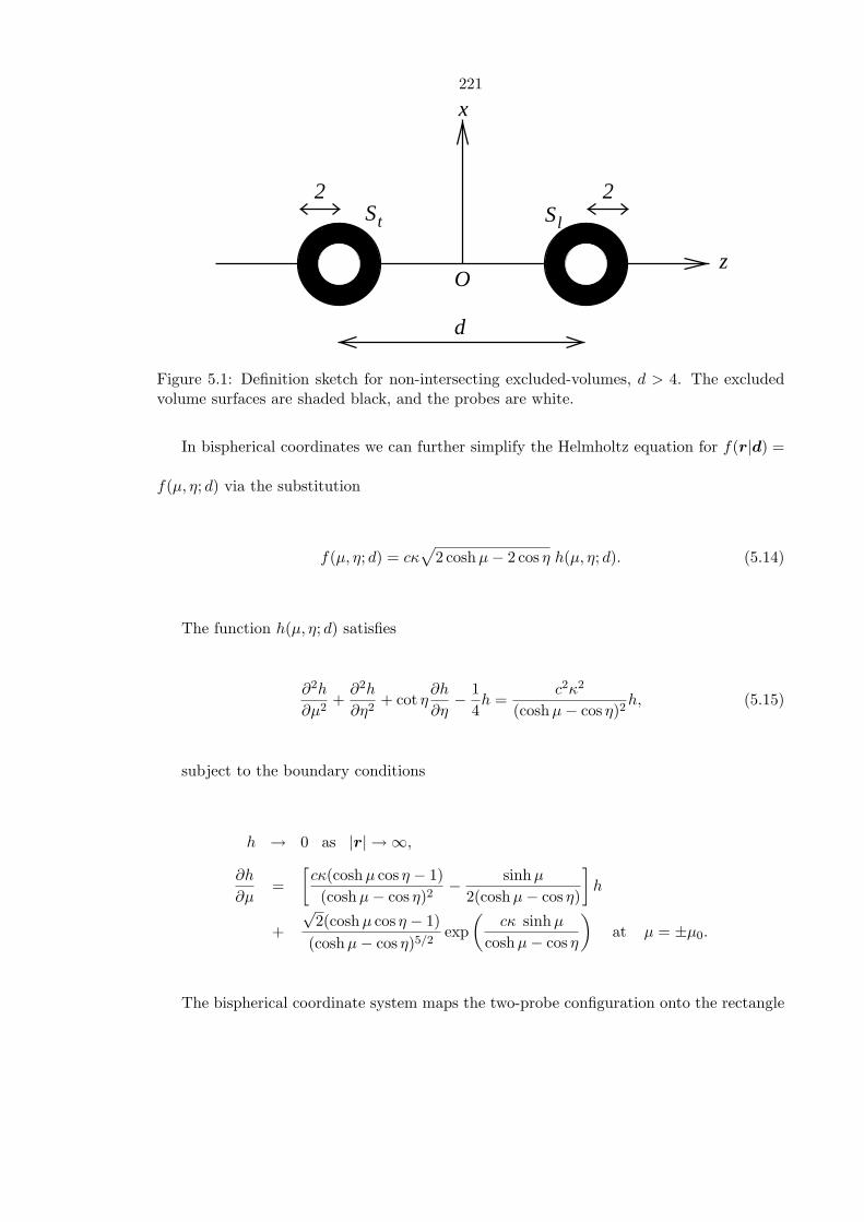
221

z

St Sl

d

O

x

22

Figure 5.1: Definition sketch for non-intersecting excluded-volumes, d > 4. The excludedvolume surfaces are shaded black, and the probes are white.

In bispherical coordinates we can further simplify the Helmholtz equation for f(r|d) =

f(µ, η; d) via the substitution

f(µ, η; d) = cκ√

2 coshµ− 2 cos η h(µ, η; d). (5.14)

The function h(µ, η; d) satisfies

∂2h

∂µ2+∂2h

∂η2+ cot η

∂h

∂η− 1

4h =

c2κ2

(coshµ− cos η)2h, (5.15)

subject to the boundary conditions

h → 0 as |r| → ∞,

∂h

∂µ=

[cκ(coshµ cos η − 1)(coshµ− cos η)2

− sinhµ2(coshµ− cos η)

]h

+√

2(coshµ cos η − 1)(coshµ− cos η)5/2

exp(

cκ sinhµcoshµ− cos η

)at µ = ±µ0.

The bispherical coordinate system maps the two-probe configuration onto the rectangle

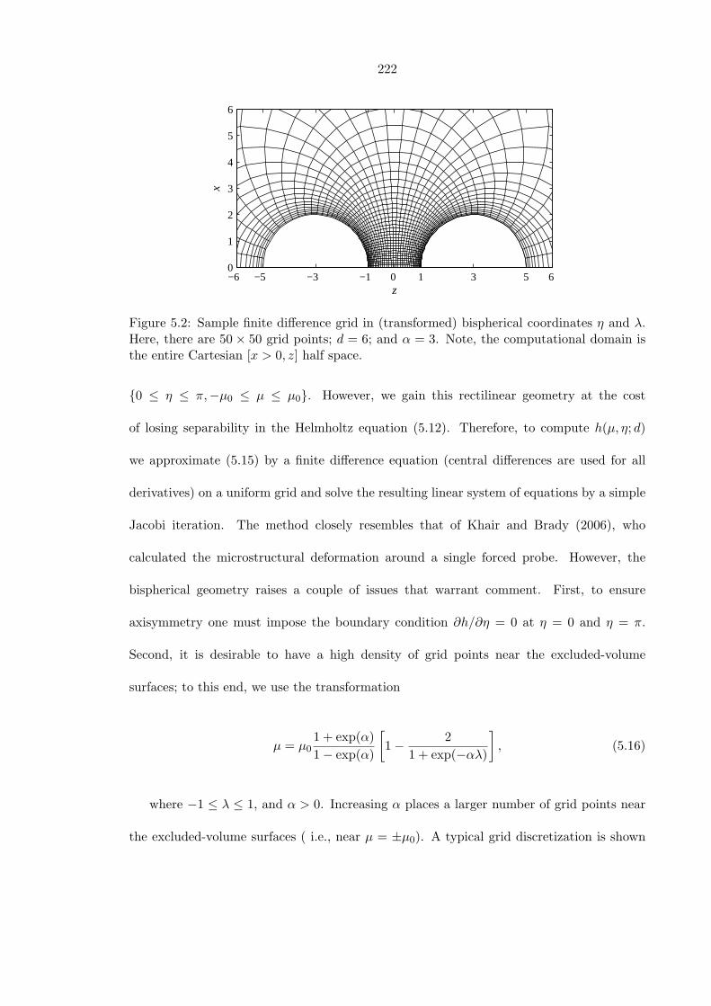
222

−6 −5 −3 −1 0 1 3 5 6 0

1

2

3

4

5

6

z

x

Figure 5.2: Sample finite difference grid in (transformed) bispherical coordinates η and λ.Here, there are 50 × 50 grid points; d = 6; and α = 3. Note, the computational domain isthe entire Cartesian [x > 0, z] half space.

0 ≤ η ≤ π,−µ0 ≤ µ ≤ µ0. However, we gain this rectilinear geometry at the cost

of losing separability in the Helmholtz equation (5.12). Therefore, to compute h(µ, η; d)

we approximate (5.15) by a finite difference equation (central differences are used for all

derivatives) on a uniform grid and solve the resulting linear system of equations by a simple

Jacobi iteration. The method closely resembles that of Khair and Brady (2006), who

calculated the microstructural deformation around a single forced probe. However, the

bispherical geometry raises a couple of issues that warrant comment. First, to ensure

axisymmetry one must impose the boundary condition ∂h/∂η = 0 at η = 0 and η = π.

Second, it is desirable to have a high density of grid points near the excluded-volume

surfaces; to this end, we use the transformation

µ = µ01 + exp(α)1− exp(α)

[1− 2

1 + exp(−αλ)

], (5.16)

where −1 ≤ λ ≤ 1, and α > 0. Increasing α places a larger number of grid points near

the excluded-volume surfaces ( i.e., near µ = ±µ0). A typical grid discretization is shown

223

in figure 5.2.

Finally, from (5.11) the entropic forces on the probes, which are in the z-direction, are

given by

〈∆F zl 〉2 =

φkT

a6 sinh2 µ0

∫ π

0g(µ0, η)

sin η(1− cos η coshµ0)(coshµ0 − cos η)3

dη,

〈∆F zt 〉2 = −φkT

a6 sinh2 µ0

∫ π

0g(−µ0, η)

sin η(1− cos η coshµ0)(coshµ0 − cos η)3

dη.

5.3.2 Intersecting excluded volumes: toroidal coordinates

When the probes are sufficiently close, d < 4, a bath particle is not able to pass between

them. In this case, the excluded-volume surfaces intersect at an angle ψ = arccos[(d2/8)−1]

(see figure 5.3) to form a dumbbell shape. To solve the Smoluchowski equation in this

geometry it is appropriate to use toroidal coordinates; we take the same Cartesian frame

as before and define the toroidal coordinates µ and η via

x =c sinhµ

coshµ− cos η, z =

c sin ηcoshµ− cos η

,

where c is a scale factor; −π ≤ η ≤ π; and 0 < µ < ∞. The surface η = η0 (η0 > 0)

is that part of a sphere of radius c/ sin η0, centered at [0,c cot η0], which is above the x− y

plane (i.e, for which z > 0). Its mirror image about the x− y plane is the surface η = −η0.

Hence, it is easy to show

c =12

√(4− d)(4 + d) , cos η0 =

d

4.

Using the substitution (5.14), in toroidal coordinates the Helmholtz equation for f(µ, η; d)

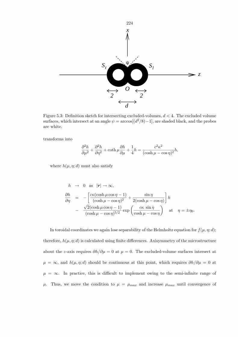
224

St Sl

z

ψ

x

O

d

2 2

Figure 5.3: Definition sketch for intersecting excluded-volumes, d < 4. The excluded volumesurfaces, which intersect at an angle ψ = arccos[(d2/8)−1], are shaded black, and the probesare white.

transforms into

∂2h

∂µ2+∂2h

∂η2+ cothµ

∂h

∂µ+

14h =

c2κ2

(coshµ− cos η)2h,

where h(µ, η; d) must also satisfy

h → 0 as |r| → ∞,

∂h

∂η= −

[cκ(coshµ cos η − 1)(coshµ− cos η)2

+sin η

2(coshµ− cos η)

]h

−√

2(coshµ cos η − 1)(coshµ− cos η)5/2

exp(

cκ sin ηcoshµ− cos η

)at η = ±η0.

In toroidal coordinates we again lose separability of the Helmholtz equation for f(µ, η; d);

therefore, h(µ, η; d) is calculated using finite differences. Axisymmetry of the microstructure

about the z-axis requires ∂h/∂µ = 0 at µ = 0. The excluded-volume surfaces intersect at

µ = ∞, and h(µ, η; d) should be continuous at this point, which requires ∂h/∂µ = 0 at

µ = ∞. In practice, this is difficult to implement owing to the semi-infinite range of

µ. Thus, we move the condition to µ = µmax and increase µmax until convergence of

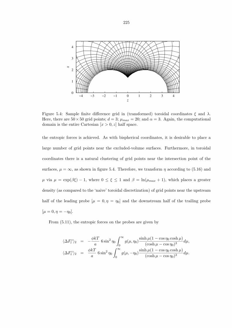
225

−4 −3 −2 −1 0 1 2 3 40

1

2

3

4

z

x

Figure 5.4: Sample finite difference grid in (transformed) toroidal coordinates ξ and λ.Here, there are 50×50 grid points; d = 3; µmax = 20; and α = 3. Again, the computationaldomain is the entire Cartesian [x > 0, z] half space.

the entropic forces is achieved. As with bispherical coordinates, it is desirable to place a

large number of grid points near the excluded-volume surfaces. Furthermore, in toroidal

coordinates there is a natural clustering of grid points near the intersection point of the

surfaces, µ = ∞, as shown in figure 5.4. Therefore, we transform η according to (5.16) and

µ via µ = exp(βξ) − 1, where 0 ≤ ξ ≤ 1 and β = ln(µmax + 1), which places a greater

density (as compared to the ‘naive’ toroidal discretization) of grid points near the upstream

half of the leading probe [µ = 0, η = η0] and the downstream half of the trailing probe

[µ = 0, η = −η0].

From (5.11), the entropic forces on the probes are given by

〈∆F zl 〉2 = −φkT

a6 sin2 η0

∫ ∞

0g(µ, η0)

sinhµ(1− cos η0 coshµ)(coshµ− cos η0)3

dµ,

〈∆F zt 〉2 =

φkT

a6 sin2 η0

∫ ∞

0g(µ,−η0)

sinhµ(1− cos η0 coshµ)(coshµ− cos η0)3

dµ.

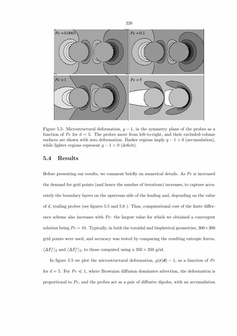
226

Pe =0.0001 Pe =0.1

Pe =1 Pe =5

Figure 5.5: Microstructural deformation, g − 1, in the symmetry plane of the probes as afunction of Pe for d = 5. The probes move from left-to-right, and their excluded-volumesurfaces are shown with zero deformation. Darker regions imply g − 1 > 0 (accumulation),while lighter regions represent g − 1 < 0 (deficit).

5.4 Results

Before presenting our results, we comment briefly on numerical details. As Pe is increased

the demand for grid points (and hence the number of iterations) increases, to capture accu-

rately the boundary layers on the upstream side of the leading and, depending on the value

of d, trailing probes (see figures 5.5 and 5.6 ). Thus, computational cost of the finite differ-

ence scheme also increases with Pe: the largest value for which we obtained a convergent

solution being Pe = 10. Typically, in both the toroidal and bispherical geometries, 300×300

grid points were used, and accuracy was tested by comparing the resulting entropic forces,

〈∆F zt 〉2 and 〈∆F z

l 〉2, to those computed using a 350× 350 grid.

In figure 5.5 we plot the microstructural deformation, g(r|d) − 1, as a function of Pe

for d = 5. For Pe 1, where Brownian diffusion dominates advection, the deformation is

proportional to Pe, and the probes act as a pair of diffusive dipoles, with an accumulation

227

of particles on their upstream sides and a deficit on their downstream sides. For sufficiently

large d the two dipoles do not interact, and the microstructure is fore-aft symmetric about

each probe. However, for smaller d (such as d = 5) the probes sense each other’s presence;

consequently, the fore-aft symmetry is broken. Moving to Pe ≈ 1, advection now comes into

play, and the deformation around the probes exhibits the beginnings of a classic boundary

layer and wake structure. Physically, in a frame fixed on the probes, the advective flux of

bath particles (moving with velocity −U) leads to an accumulation on the upstream sides

of the (impenetrable) probes, which act as obstacles that the bath particles must navigate.

The mechanism for passing around the probes is via Brownian diffusion. Thus, the boundary

layers signify a balance between advection, in transporting bath particles toward the probes,

and diffusion. On the downstream sides of the probes advection carries bath particles away;

a region of low particle density, or wake, is formed. As Pe is increased further the stronger

advective flux results in thinner boundary layers and longer wakes. Note, the boundary

layer on the trailing probe is significantly less particle-rich as compared to the leading

probe [which has an O(Pe) accumulation], as the trailing probe travels in the (low particle

density) wake created by the leading probe, while the leading probe moves through the

undisturbed dispersion. Of course, for d much larger than the characteristic wake length

(which grows as Pe) one expects the boundary layers on the trailing and leading probes

to be almost identical. Conversely, for d much smaller than the wake length the boundary

layer on the trailing probe disappears; essentially, it moves through a particle-free tunnel

of suspending fluid.

In figure 5.6 we plot the microstructural deformation as a function of Pe for d = 3. In

this case, and for all d < 4, the excluded-volume surfaces, St and Sl, of the probes join and,

from the bath particle’s viewpoint, form a single dumbbell shaped obstacle. At small Pe

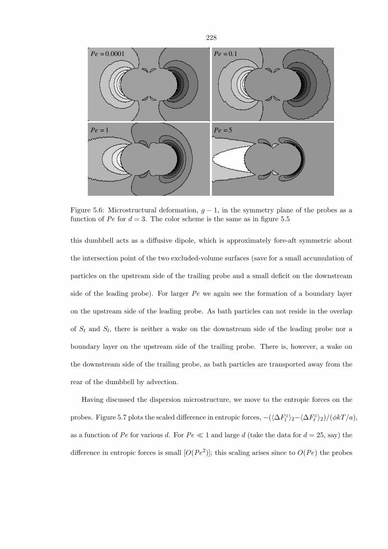
228

Pe =0.1

Pe =1

Pe =0.0001

Pe =5

Figure 5.6: Microstructural deformation, g − 1, in the symmetry plane of the probes as afunction of Pe for d = 3. The color scheme is the same as in figure 5.5

this dumbbell acts as a diffusive dipole, which is approximately fore-aft symmetric about

the intersection point of the two excluded-volume surfaces (save for a small accumulation of

particles on the upstream side of the trailing probe and a small deficit on the downstream

side of the leading probe). For larger Pe we again see the formation of a boundary layer

on the upstream side of the leading probe. As bath particles can not reside in the overlap

of St and Sl, there is neither a wake on the downstream side of the leading probe nor a

boundary layer on the upstream side of the trailing probe. There is, however, a wake on

the downstream side of the trailing probe, as bath particles are transported away from the

rear of the dumbbell by advection.

Having discussed the dispersion microstructure, we move to the entropic forces on the

probes. Figure 5.7 plots the scaled difference in entropic forces, −(〈∆F zl 〉2−〈∆F z

t 〉2)/(φkT/a),

as a function of Pe for various d. For Pe 1 and large d (take the data for d = 25, say) the

difference in entropic forces is small [O(Pe2)]; this scaling arises since to O(Pe) the probes

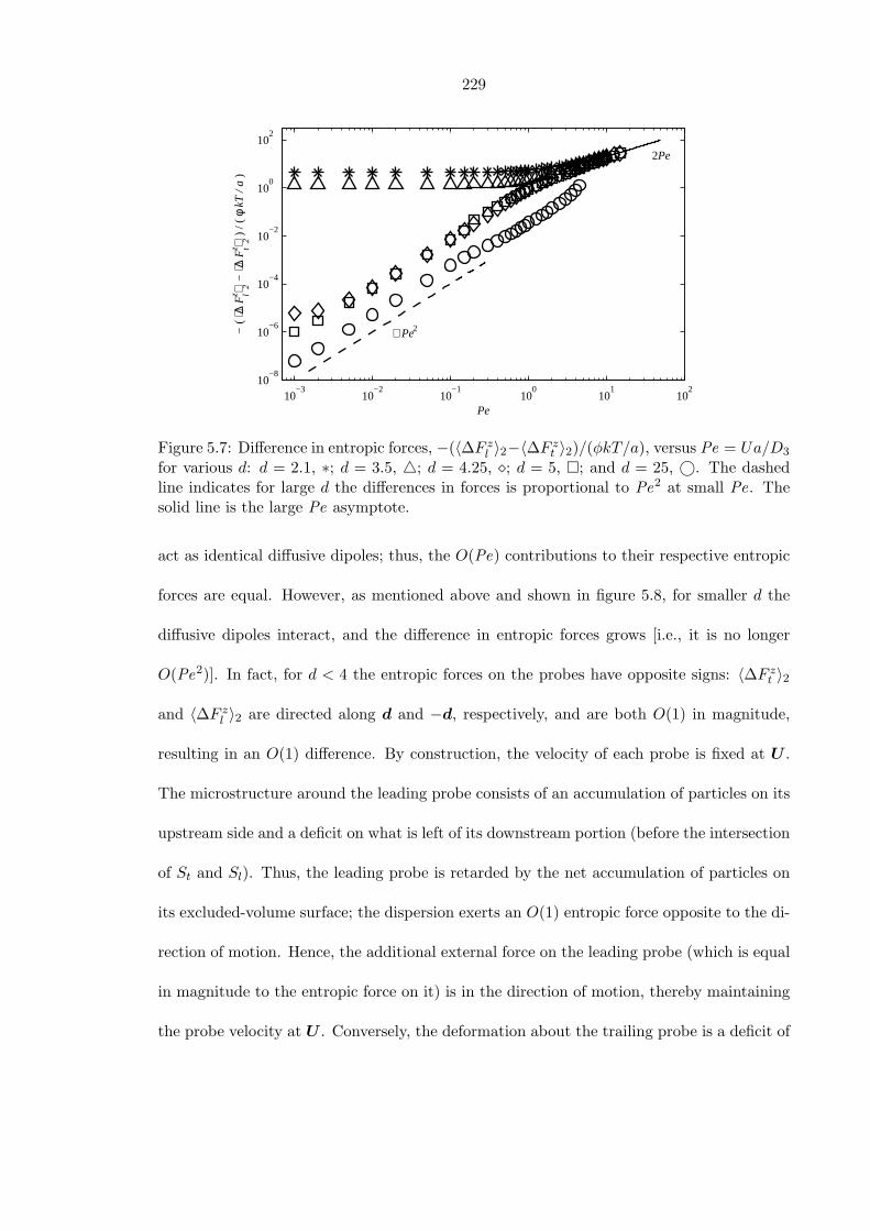
229

10−3

10−2

10−1

100

101

102

10−8

10−6

10−4

10−2

100

102

Pe

− (

⟨∆ F

z l⟩ 2 − ⟨∆

Fz t⟩ 2 )

/ (

φ kT

/ a

)

∼ Pe2

2Pe

Figure 5.7: Difference in entropic forces, −(〈∆F zl 〉2−〈∆F z

t 〉2)/(φkT/a), versus Pe = Ua/D3

for various d: d = 2.1, ∗; d = 3.5, 4; d = 4.25, ; d = 5, ; and d = 25, ©. The dashedline indicates for large d the differences in forces is proportional to Pe2 at small Pe. Thesolid line is the large Pe asymptote.

act as identical diffusive dipoles; thus, the O(Pe) contributions to their respective entropic

forces are equal. However, as mentioned above and shown in figure 5.8, for smaller d the

diffusive dipoles interact, and the difference in entropic forces grows [i.e., it is no longer

O(Pe2)]. In fact, for d < 4 the entropic forces on the probes have opposite signs: 〈∆F zt 〉2

and 〈∆F zl 〉2 are directed along d and −d, respectively, and are both O(1) in magnitude,

resulting in an O(1) difference. By construction, the velocity of each probe is fixed at U .

The microstructure around the leading probe consists of an accumulation of particles on its

upstream side and a deficit on what is left of its downstream portion (before the intersection

of St and Sl). Thus, the leading probe is retarded by the net accumulation of particles on

its excluded-volume surface; the dispersion exerts an O(1) entropic force opposite to the di-

rection of motion. Hence, the additional external force on the leading probe (which is equal

in magnitude to the entropic force on it) is in the direction of motion, thereby maintaining

the probe velocity at U . Conversely, the deformation about the trailing probe is a deficit of

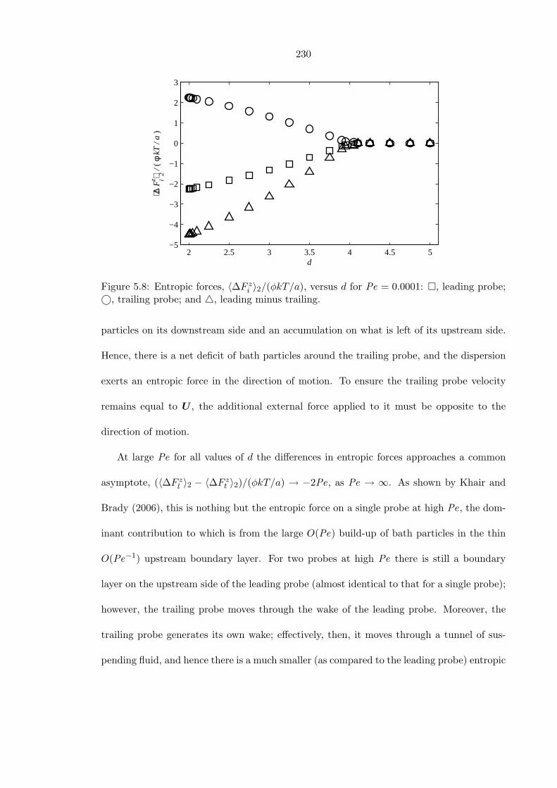
230

2 2.5 3 3.5 4 4.5 5−5

−4

−3

−2

−1

0

1

2

3

d

⟨∆ F

z i⟩ 2 / (

φ kT

/ a

)

Figure 5.8: Entropic forces, 〈∆F zi 〉2/(φkT/a), versus d for Pe = 0.0001: , leading probe;

©, trailing probe; and 4, leading minus trailing.

particles on its downstream side and an accumulation on what is left of its upstream side.

Hence, there is a net deficit of bath particles around the trailing probe, and the dispersion

exerts an entropic force in the direction of motion. To ensure the trailing probe velocity

remains equal to U , the additional external force applied to it must be opposite to the

direction of motion.

At large Pe for all values of d the differences in entropic forces approaches a common

asymptote, (〈∆F zl 〉2 − 〈∆F z

t 〉2)/(φkT/a) → −2Pe, as Pe → ∞. As shown by Khair and

Brady (2006), this is nothing but the entropic force on a single probe at high Pe, the dom-

inant contribution to which is from the large O(Pe) build-up of bath particles in the thin

O(Pe−1) upstream boundary layer. For two probes at high Pe there is still a boundary

layer on the upstream side of the leading probe (almost identical to that for a single probe);

however, the trailing probe moves through the wake of the leading probe. Moreover, the

trailing probe generates its own wake; effectively, then, it moves through a tunnel of sus-

pending fluid, and hence there is a much smaller (as compared to the leading probe) entropic

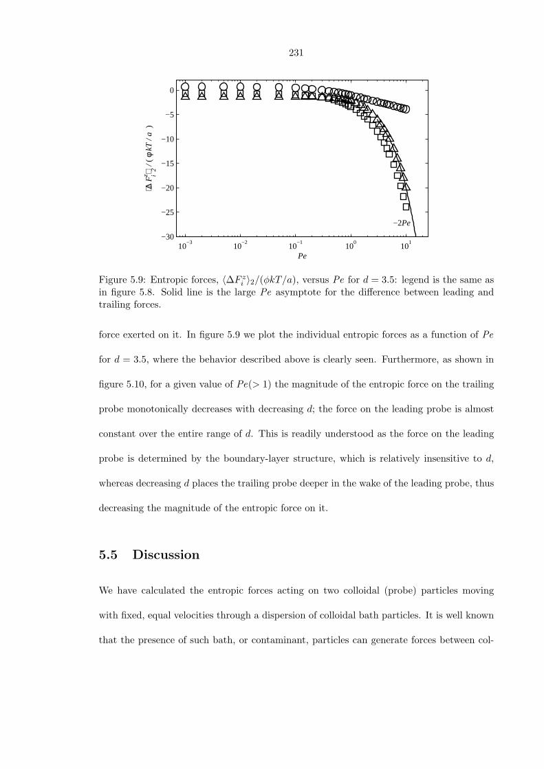
231

10−3

10−2

10−1

100

101

−30

−25

−20

−15

−10

−5

0

Pe

⟨∆ F

z i⟩ 2 / (

φ kT

/ a

)

−2Pe

Figure 5.9: Entropic forces, 〈∆F zi 〉2/(φkT/a), versus Pe for d = 3.5: legend is the same as

in figure 5.8. Solid line is the large Pe asymptote for the difference between leading andtrailing forces.

force exerted on it. In figure 5.9 we plot the individual entropic forces as a function of Pe

for d = 3.5, where the behavior described above is clearly seen. Furthermore, as shown in

figure 5.10, for a given value of Pe(> 1) the magnitude of the entropic force on the trailing

probe monotonically decreases with decreasing d; the force on the leading probe is almost

constant over the entire range of d. This is readily understood as the force on the leading

probe is determined by the boundary-layer structure, which is relatively insensitive to d,

whereas decreasing d places the trailing probe deeper in the wake of the leading probe, thus

decreasing the magnitude of the entropic force on it.

5.5 Discussion

We have calculated the entropic forces acting on two colloidal (probe) particles moving

with fixed, equal velocities through a dispersion of colloidal bath particles. It is well known

that the presence of such bath, or contaminant, particles can generate forces between col-

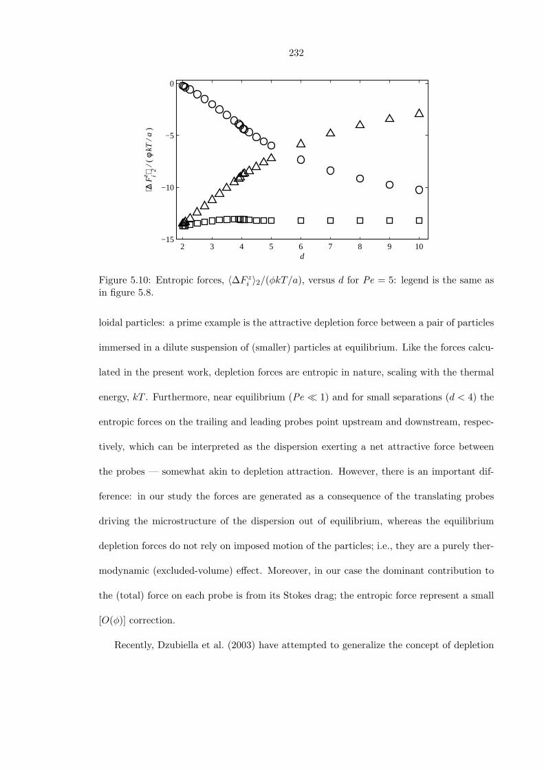
232

2 3 4 5 6 7 8 9 10−15

−10

−5

0

d

⟨∆ F

z i⟩ 2 / (

φ kT

/ a

)

Figure 5.10: Entropic forces, 〈∆F zi 〉2/(φkT/a), versus d for Pe = 5: legend is the same as

in figure 5.8.

loidal particles: a prime example is the attractive depletion force between a pair of particles

immersed in a dilute suspension of (smaller) particles at equilibrium. Like the forces calcu-

lated in the present work, depletion forces are entropic in nature, scaling with the thermal

energy, kT . Furthermore, near equilibrium (Pe 1) and for small separations (d < 4) the

entropic forces on the trailing and leading probes point upstream and downstream, respec-

tively, which can be interpreted as the dispersion exerting a net attractive force between

the probes — somewhat akin to depletion attraction. However, there is an important dif-

ference: in our study the forces are generated as a consequence of the translating probes

driving the microstructure of the dispersion out of equilibrium, whereas the equilibrium

depletion forces do not rely on imposed motion of the particles; i.e., they are a purely ther-

modynamic (excluded-volume) effect. Moreover, in our case the dominant contribution to

the (total) force on each probe is from its Stokes drag; the entropic force represent a small

[O(φ)] correction.

Recently, Dzubiella et al. (2003) have attempted to generalize the concept of depletion

233

forces to nonequilibrium, by computing the entropic forces on two stationary probes in a

stream of smaller bath particles. When the bath particles flow along the line of centers of the

probes, for moderate stream velocities they find [see their figure 3(b)] that the magnitude

of the force on the trailing probe is less than that on the leading probe, in agreement with

our results for Pe > 1 (see figure 5.10). However, unlike us, they do not report a change

in direction of the entropic force on the trailing probe with increasing Pe for d < 4 (see

figure 5.9). Although Dzubiella et al. (2003) investigated more general (non-axisymmetric)

probe configurations, their analytical methods (as discussed in § 5.1) are restricted to widely

separated particles and small stream velocities. We, on the other hand, have computed the

nonequilibrium microstructure and entropic forces for all (axisymmetric) separations and

probe velocities.

In this study, we neglected hydrodynamic interactions between particles. Although, as

mentioned in § 5.1, there exist experimental systems for which this is a reasonable assump-

tion, one should pause and consider their effect. For example, in the absence of hydro-

dynamic interactions at large Pe the entropic force on the trailing probe vanishes, while

the entropic force on the leading probe approaches the single probe limit (see figure 5.7).

However, with hydrodynamic interactions this may not be so. For, as discussed by Khair

and Brady (2006), in the limit of infinite Pe the microstructure around a single moving

probe attains spherical symmetry, i.e., the upstream boundary layer wraps over the entire

(excluded-volume) surface of the probe, and the wake disappears. Physically, this occurs as

bath particles from upstream ‘stick’ to the probe (due to hydrodynamic lubrication forces)

as they are advected around it. Consequently, the force on the probe has equal contributions

from the pushing of bath particles upstream of it and pulling of particles downstream of it.

(Note, at infinite Pe the force exerted by the dispersion on the probe is hydrodynamic, not

234

entropic, in origin.) Now, imagine two probes in the presence of hydrodynamic interactions

at large Pe. The leading probe no longer creates a wake for the trailing probe to move

through; likewise, the trailing probe does not create a wake of its own. We expect this

qualitative change in the microstructure at large Pe due to hydrodynamic interactions to

be reflected in the computed forces. However, the inclusion of hydrodynamic interactions is

beyond the scope of analytical theory, and one must resort to computer simulations, such

as Stokesian Dynamics.

The theoretical framework developed in § 5.2 may be used to study other interesting

problems. A natural extension is to consider two probes moving perpendicular to their

line of centers, for which the microstructural deformation is no longer axisymmetric about

their separation, d. Consequently, we expect the entropic forces on the (top and bottom)

probes to have components parallel and perpendicular to d. For large d = |d| the parallel

components for each probe vanish, while the perpendicular components are, by symmetry,

identical and equal to that for a single moving probe. For smaller d (close to, but greater

than 4) a bath particle is just able to squeeze between the probes. The perpendicular

components for each probe remain identical, but are now not equal to that for a single

probe. In contrast, the parallel components should be in opposite directions: the parallel

forces on the top and bottom probes point upward and downward, respectively, which may

be viewed as the dispersion exerting a net repulsive force between the probes. Indeed,

this behavior was seen by Dzubiella et al. (2003) [see their figure 3(a)]. Furthermore, as

mentioned in § 5.1, our theory can be easily extended to study the small bath particle limit

of Dzubiella et al. (2003), which is somewhat more representative of experimental studies

on depletion forces. Lastly, the Smoluchowski equation (5.3) applies when there is relative

motion between the probes. Hence, for example, it can be used to study the motion of a

235

probe at fixed velocity approaching a stationary wall (which is, of course, just a probe of

infinite radius): a simple problem, which could provide a starting point for investigating

the patterning of surfaces using driven colloidal particles.

On a complementary note to the present study, one could fix the external forces on

the probes and calculate their average velocities. Although qualitatively similar, there are

important (and subtle) differences between the fixed-force and fixed-velocity cases; indeed,

the formulation of the three-body Smoluchowski equation for the fixed-force problem is more

involved. Nevertheless, one can arrive at an equation for the conditional pair-distribution

function analogous to (5.6), in the limit where the bath particles are much more mobile

(i.e., they have a far higher diffusivity) than the probes, which, in turn, requires the bath

particles to be much smaller than the probes. As a first study, it would be wise to consider

two (large) probes forced along their line of centers, d, for which their average velocities will

be directed along d, also. For Pe > 1 (here, Pe is defined as the dimensionless external force

on the probes) and d > 4 the trailing probe would move through the wake created by the

leading probe, which is practically devoid of bath particles. Furthermore, the trailing probe

generates its own wake; hence, as per the fixed-velocity problem, it travels through a tunnel

of suspending fluid. In contrast, the leading probe is retarded by the need to push bath

particles out of its path. As such, one expects, in general, that the trailing probe moves

faster than the leading probe, and it may eventually ‘catch-up’ and contact the leading

probe. Continuing this process, one may add a second trailing probe (this is, unfortunately,

beyond the realm of analytical theory; one must employ computer simulations), which will

catch-up to the first trailing and leading probes. In this way, by adding yet more probes,

one may form a ‘train’ of probes moving through the dispersion, which could provide a route

for pattern formation in colloidal dispersions, and perhaps other complex materials. We

236

shall, however, leave this fascinating world of multi-particle interactions for future studies.

237

5.6 Bibliography

V. J. Anderson and H. N. W. Lekkerkerker. Insights into phase transition kinetics from

colloid science. Nature, 416:811–815, 2002.

S. Asakura and F. Oosawa. On interaction between two bodies immersed in a solution of

macromolecules. J. Chem. Phys., 22:1255–1256, 1958.

J. Chakrabarti, J. Dzubiella, and Lowen. Reentrance effect in the lane formation of driven

colloids. Phys. Rev. E, 70:012401, 2004.

J. C. Crocker, J. A. Matteo, A. D. Dinsmore, and A. G. Yodh. Entropic attraction and

repulsion in binary colloids probed with a line optical tweezer. Phys. Rev. Lett., 82:

4352–4355, 1999.

J. Dzubiella, G. P. Hoffman, and H. Lowen. Lane formation in colloidal mixtures driven by

an external field. Phys. Rev. E, 65:021402, 2002.

J. Dzubiella, H. Lowen, and C. N. Likos. Depletion forces in nonequilibrium. Phys. Rev.

Lett., 91:248301, 2003.

L. Heldon, R. Roth, G. H. Koenderink, P. Leiderer, and C. Bechinger. Direct measurement

of entropic forces induced by rigid rods. Phys. Rev. Lett., 90:048301, 2003.

P. Jenkins and M. Snowden. Depletion flocculation in colloidal dispersions. Adv. Colloid

Interface Sci., 68:57–96, 1996.

P. D. Kaplan, J. L. Rouke, A. G. Yodh, and D. G. Pine. Entropically driven surface phase

separation in binary colloidal mixtures. Phys. Rev. Lett., 72:582–585, 1994.

238

A. S. Khair and J. F. Brady. Single particle motion in colloidal dispersions: A simple model

for active and nonlinear microrheology. J. Fluid Mech., 557:73–117, 2006.

P. Moon and D. M. Spencer. Field theory handbook: including coordinate systems, differ-

ential equations, and their solutions. Springer, 1961.

P. M. Morse and H. Feshbach. Methods of theoretical physics. Part II. McGraw-Hill, 1953.

T. M. Squires and J. F. Brady. A simple paradigm for active and nonlinear microrheology.

Phys. Fluids, 17:073101, 2005.

R. Tehver, A. Maritan, J. Koplik, and J. R. Banavar. Depletion forces in hard-sphere

colloids. Phys. Rev. E, 59:R1339, 1999.

R. Verma, J. C. Crocker, T. C. Lubensky, and A. G. Yodh. Entropic colloidal interactions

in concentrated DNA solutions. Phys. Rev. Lett., 81:4004–4007, 1998.

A. G. Yodh, L. Keng-Hui, J. C. Crocker, A. D. Dinsmore, R. Verma, and P. D. Kaplan.

Entropically driven self-assembly and interaction in suspension. Phil. Trans. R. Soc. A.,

359:921–937, 2001.

239

Chapter 6

Conclusions

240

6.1 Conclusions & future directions

Over the past decade, microrheology has emerged as a technique to interrogate and manip-

ulate complex fluids and biological materials at the microstructural scale. While advances

in experimental microrheology methods continue unabated, theoretical developments, in

general, struggle to keep pace. To address this imbalance, we have studied a prototypical

model for active (nonlinear) microrheology: an externally driven ‘probe’ particle immersed

in a hard-sphere dispersion of colloidal ‘bath’ particles. The hard-sphere colloidal dispersion

is, perhaps, the ‘simplest’ of complex fluids; nevertheless, as shown in the previous chapters,

its microrheological properties are nontrivial and require careful analysis.

In chapter 2 we investigated a probe traveling at fixed external force. The motion of

the probe drives the microstructure of the dispersion out of equilibrium; counteracting this

is the Brownian diffusion of the probe and bath particles. The degree of microstructural

distortion is set by the dimensionless external force on the probe, or Peclet number, Pe.

With the nonequilibrium microstructure in hand, we calculate the average translational

velocity of the probe, and from the average velocity one can infer a ‘microviscosity’ of the

dispersion via Stokes drag law. In particular, we demonstrated that at large Pe particles

experiencing short-ranged hydrodynamic lubrication interactions give a microviscosity that

increases, or ‘force-thickens’. This is reminiscent of the ‘shear-thickening’ at large Pe (with

Pe the non-dimensional shear rate) observed in macrorheology (Bergenholtz et al. 2002).

Indeed, after appropriate scaling, we were able to make a quantitative comparison (see

figure 2.18). Shear-thickening complex fluids have recently been employed in the design

of military armor (Lee et al. 2003); the onset and degree of thickening of the micro- (and

macro-) viscosity are key design parameters. How do they vary with probe-bath size ratio

241

and probe pulling mode (fixed force versus fixed velocity)? Is the ‘correct’ size ratio for

microrheology experiments that which gives a (scaled) onset and degree equal to that for

the macroviscosity? For dilute systems these questions may be answered by extending the

theoretical framework developed in chapter 2, while for concentrated dispersions (where

one has to accurately account for the long-ranged, many-body hydrodynamic interactions

between particles) the Stokesian Dynamics paradigm (Brady and Bossis 1988) is applicable.

In chapter 3 we considered a probe subjected to a small amplitude (Pe 1) oscillatory

force. In this case, the microviscosity has components in-phase (liquid-like) and out-of

phase (solid-like) with the external forcing — a signature response of viscoelastic fluids.

By computing the microviscosity as a function of oscillation frequency ω of the probe we

were able to delineate the (linear) ‘microviscoelastic’ response of the dispersion. Again,

after appropriate scaling, the micro results are in agreement with the equivalent macro

measurements (see figures 3.2 and 3.3).

Nanometer scale interparticle forces play a crucial role in the stability, phase behav-

ior, and rheology of colloidal dispersions (Wagner and Bender 2004). For instance, shear-

thickening can be eliminated by suitable ‘tuning’ of these forces (Bergenholtz et al. 2002).

In microrheology, the equivalent effect is the inhibition of force-thickening; however, only

the hard-sphere ‘excluded-annulus’ model has been utilized to study this (see chapter 2).

Thus, we need to apply the theory developed in chapter 2 to more realistic (e.g., Van der

Waals, DLVO) interparticle forces. The inverse problem is also interesting; namely, can

microrheology be used to infer nano-scale interparticle interactions? In macrorheology the

answer is yes: for example, high-frequency measurements of the elastic modulus have been

employed to determine the surface charge of electrostatically stabilized dispersions (Horn

et al., 2000). Furthermore, the elastic modulus has been used to quantify the roughness,

242

or surface-slip, at particle surfaces (Fritz et al., 2002). In chapter 3 we showed that the

elastic modulus diverges like ω1/2 as ω →∞ for particles interacting via excluded-annulus

interparticle forces. On the other hand, in the absence of hard-sphere interparticle forces

the effect of hydrodynamic interactions yields a finite elastic modulus as ω →∞. The for-

malism of chapter 3 may easily be extended to study the effect of more specific, or realistic,

interparticle forces on the high-frequency behavior of the elastic modulus.

In chapter 4 we investigated an issue that has hitherto been untouched by the (micro-)

rheological community: namely, what role does the shape of the probe play. For microrhe-

ology, this is a rare occurrence of theoretical analysis preceding experimental measurement.

Specifically, we considered the probe to be a body of revolution with major and minor semi-

axes a and b, respectively, translating at constant velocity through a dispersion of spherical

bath particles (of radii b). The probe’s shape is such that when it’s major(minor) axis is the

axis of revolution the excluded-volume, or contact, surface between it and a bath particle is

a prolate(oblate) spheroid. For a probe moving along its symmetry axis, the microviscosity

was computed as a function of the aspect ratio of the probe, a = a/b, thereby delineating

the role of the probe’s shape. For a prolate probe, regardless of the value of a, the microvis-

cosity monotonically decreases, or ‘velocity-thins’, from a Newtonian plateau at small Pe

(here, Pe is the non-dimensional velocity of the probe) until a second Newtonian plateau

is reached as Pe → ∞. For an oblate probe, the microviscosity again transitions between

two Newtonian plateaus: for a < 3.52 (to two decimal places) the microviscosity at small

Pe is greater than at large Pe (velocity-thinning); however, for a > 3.52 the microviscosity

at small Pe is less than at large Pe, which suggests it ‘velocity-thickens’ as Pe is increased.

This anomalous velocity-thickening — due entirely to the probe shape — highlights the

care needed when conducting microrheology experiments with non-spherical probes.

243

One of the main limitations of microrheology with a single spherical probe is that one

can determine only a (scalar) microviscosity of a material. In contrast, macrorheology can,

in principle, obtain the full stress tensor including normal stress differences and an isotropic

osmotic pressure (Bergenholtz et al. 2002). Could a non-spherical probe give more than

just a microviscosity? In chapter 4 we presented a preliminary analysis of this question, by

considering a prolate probe that translates at an angle β to its symmetry axis. In general,

one must apply an external torque to the probe to prevent it from rotating. In the linear-

response (Pe 1) regime the dispersion does not exert a torque of the probe; consequently,

the external torque is zero. However, far from equilibrium (Pe 1) the dispersion does

exert a torque on the probe that, in the absence of an external torque, would orient the

probe in a broadside (β = π/2) configuration. From Leal’s (Leal 1975) investigation on

the translation of rod-like particles in a second-order fluid, a stable broadside configuration

suggests that the quantity 4N1 + N2 < 0 (N1 and N2 are the first and second normal

stress differences, respectively) at large Pe. Within the ‘radial-balance’ approximation used

to compute the microstructure at large Pe, this is consistent with the macrorheological

findings of Brady and Morris (1997). However, as discussed in chapter 4, one must solve

the ‘full’ microstructural problem at large Pe before any definitive conclusions can be drawn.

Moreover, as shown by Zarraga et al. (2000) and mentioned in § 4.7, it is not clear that the

second-order fluid is a ‘correct’ model for colloidal dispersions at large Pe; hence, it may not

be appropriate to infer normal stress differences from our model by comparison to Leal’s

(Leal 1975) results.

The discussion above does, nevertheless, highlight an important point: the non-viscometric

flow generated by a prolate probe implies that one can determine only the combination

4N1 +N2, and not N1 and N2 in isolation. In contrast, macrorheology utilizes viscometric

244

flows (simple shear, plane strain etc.), from which can yield separate measurements of N1

and N2. Thus, the challenge for microrheologists is to develop techniques that are capable

of ascertaining normal stress differences independently.

In a broader context, microrheology is faced with several important challenges. For

example, passive microrheology has been applied recently to characterizing the heteroge-

neous environment within living cells (Daniels et al. 2006). In fact, the in vivo application

of microrheology to living cells has been given its own name: ‘Bio-microrheology’ (Weihs

et al. 2006). In modeling this problem one must account for the interaction of the diffusing

probe with the cell walls. More generally, how do the boundaries of a sample affect its

microrheologically-measured properties? Could, for example, the change in microviscosity

with probe position be used to construct a ‘rheological map’ of a cell? Simple low-Reynolds-

number hydrodynamics tells us the force (and hence microviscosity) required to bring a

particle close to a rigid wall diverges in the limit of contact. Can microrheology pick up on

this? How does the elasticity and deformation of the cell wall come into play?

An interface between two materials (a cell membrane, for instance) is another type of

boundary that presents challenges and opportunities for (micro-)rheologists. Very recently,

the first passive interfacial microrheology studies have been reported (Anguelouch et al.

2006; Oetama and Walz 2006; Prasad et al. 2006). We are faced with many issues when an

active probe is placed near or at an interface: What exactly is being measured? An inter-

facial (surface) microviscosity? Some combination of the microviscosities of the materials

either side of the interface? What shape and size should the probe be? How far does the

probe have to be inside one material so that it does not ‘see’ the interface? Does the motion

of the probe deform the interface? The theoretical techniques developed in this thesis can

serve as a sound starting point to tackle these interesting problems.

245

At the theoretical and computational levels, we need to extend our current models of

microrheology to accurately describe more intricately microstructured materials, such as

fibrous networks and gels. For example, yield-stress like behavior has been observed in

active microrheology experiments of colloidal dispersions near the glass transition (Habdas

et al. 2004); the existing (dilute) theories simply can’t capture this.

In chapter 5 we considered the motion of two ‘probe’ particles traveling at constant,

equal velocities through a hard-sphere dispersion, in an attempt to study entropic depletion

forces out of equilibrium. The physical picture is simple: the moving probes disturb the

tranquility of the dispersion; in response, the dispersion exerts a reactive entropic force

on each probe, which depends on the non-dimensional velocity of the probes (i.e., the

Peclet number, Pe) and their separation. When moving slowly (Pe 1) we recover the

(equilibrium) depletion attraction between probes. For rapid motion (Pe 1) the leading

probe does all the work in pushing bath particles out of its path, while the trailing probe

gets a ‘free ride’. Hence, the entropic force on the trailing probe vanishes, whereas the force

on the leading probe approaches a limiting value equal to that for a single probe moving at

large Pe. Conversely, if the probes moved with equal applied forces the trailing probe would,

on average, move faster than the leading probe and eventually catch-up to it. By adding

more (trailing) probes one may form a ‘train’ of particles moving through the dispersion,

which constitutes a mechanism for pattern formation in complex fluids.

The discussion above points up many interesting questions: What happens if the probes

move with different speeds? How do non-equilibrium depletion forces depend on the probe-

bath size ratio? And how are they affected by interparticle forces (beyond hard-sphere

repulsion) between the probes? What if the probes do not move along their line of centers?

How many particles can one add to a colloidal ‘train’ before it buckles? Is the train stable

246

to small amplitude perturbations? These problems need to be addressed via analytical

theory (by extending the formalism developed in chapter 5), computer simulations, and

experiments. A possible experimental setup is to hold two (or more) colloidal particles at

a fixed separation using optical traps and flow a complex fluid past them (via a translating

stage). The entropic (depletion) force exerted on each probe is simply the negative of the

force required to trap it (less the hydrodynamic drag).

Finally, we note that entropic attraction can be induced between not only colloidal

particles but also particles and walls. Specifically, by geometric patterning of a surface

one can create an ‘entropic force field’ useful in the self-assembly of colloids in a desired

fashion (Dinsmore et al. 1996). Existing studies have been restricted to equilibrium systems;

however, one can imagine that in a microfluidic device, for example, colloidal particles may

be actively transported (driven) past a templated surface, and one needs to take account of

this nonequilibrium forcing. The formalism of chapter 5 is readily applicable to study the

motion of a colloid probe in the proximity of a rigid wall. The goal would be to determine the

forces on the driven colloid and the wall as a function of the surface patterning, separation,

and colloid motion (i.e., parallel or perpendicular to the wall).

247

6.2 Bibliography

A. Anguelouch, R. L. Leheny, and D. H. Reich. Application of ferromagnetic nanowires to

interfacial microrheology. Appl. Phys. Lett., 89:111914, 2006.

J. Bergenholtz, J. F. Brady, and M. Vicic. The non-Newtonian rheology of dilute colloidal

suspensions. J. Fluid Mech., 456:239–275, 2002.

J. F. Brady and G. Bossis. Stokesian dynamics. Annu. Rev. Fluid. Mech., 20:111–157, 1988.

J. F. Brady and J. F. Morris. Microstructure of strongly sheared suspensions and its impact

on rheology and diffusion. J. Fluid Mech., 348:103–139, 1997.

B. R. Daniels, B. C. Masi, and D. Wirtz. Probing single-cell micromechanics in vivo: the

micorheology of C. elegans developing embryos. Biophys. J., 90:4712–4719, 2006.

A. D. Dinsmore, A. G. Yodh, and D. J. Pine. Entropic control of particle motion using

passive surface microstructures. Nature, 383:239–242, 1996.

G. Fritz, B. J. Maranzano, N. J. Wagner, and N. Willenbacher. High frequency rheology of

hard sphere colloidal dispersions measured with a torsional resonator. J. Non-Newtonian

Fluid Mech., 102:149–156, 2002.

P. Habdas, D. Schaar, A. C. Levitt, and E. R. Weeks. Forced motion of a probe particle

near the colloidal glass transition. Europhys. Lett., 79:477–483, 2004.

F. M. Horn, W. Richtering, J. Bergenholtz, N. Willenbacher, and N. J. Wagner. Hydro-

dynamic and colloidal interactions in concentrated charge-stabilized polymer dispersions.

J. Coll. Int. Sci., 225:166–178, 2000.

248

L. G. Leal. The slow motion of a slender rod-like particle in a second-order fluid. J. Fluid

Mech., 69:305–337, 1975.

Y. S. Lee, E. D. Wetzel, and N. J. Wagner. The ballistic impact characterists of Kevlar

woven fabrics impregnated with a colloidal shear thickening fluid. J. Mater. Sci., 38:

2825–2833, 2003.

R. J. Oetama and R. Y. Walz. Investigation of short-time particle dynamcs near an interface

in the presence of nonadsorbed macro-ions. Langmuir, 22:8318–8325, 2006.

V. Prasad, S. A. Koehler, and E. R. Weeks. Two-particle microrheology of quasi-2d systems.

Phys. Rev. Lett., 97:176001, 2006.

N. J. Wagner and J. W. Bender. The role of nanoscale forces in colloid dispersion rheology.

MRS Bulletin, 29:100–106, 2004.

D. Weihs, T. G. Mason, and M. A. Teitell. Bio-microrheology: A frontier in microrheology.

Biophys. J., 91:4296–4305, 2006.

I. E. Zarraga, D. A. Hill, and D. T. Leighton. The characterization of the total stress

of concentrated suspensions of noncolloidal spheres in Newtonian fluids. J. Rheol., 44:

185–220, 2000.