Peer Effects in Science: Evidence from the Dismissal of Scientists in Nazi Germany

“rdr029” — 2012/4/17 — 12:44 — page 838 — #1

Review of Economic Studies (2012)79, 838–861 doi: 10.1093/restud/rdr029 The Author 2011. Published by Oxford University Press on behalf of The Review of Economic Studies Limited.Advance access publication 18 November 2011

PeerEffects in Science:Evidence from the Dismissal of

Scientists in Nazi GermanyFABIAN WALDINGER

University of Warwick

First version received July2010; final version accepted June2011 (Eds.)

This paper analyses peer effects among university scientists. Specifically, it investigates whetherthe quality and the number of peers affect the productivity of researchers in physics, chemistry, andmathematics. The usual endogeneity problems related to estimating peer effects are addressed by usingthe dismissal of scientists by the Nazi government in 1933 as a source of exogenous variation in thepeer group of scientists staying in Germany. To investigate localized peer effects, I construct a new paneldata set covering the universe of scientists at the German universities from 1925 to 1938 from historicalsources. I find no evidence for peer effects at the local level. Even very high-quality scientists do notaffect the productivity of their local peers.

Key words: Peer effects, Academics, Nazi Germany, Jewish scientists, Scientific productivity

JEL Codes: I20, I23, I28, J15, J24, N34, N44

1. INTRODUCTION

It is widely believed that localized peer effects are important among academic researchers. In-dividual researchers do not necessarily take these effects into account when they decide whereto locate. This may result in misallocation of talent and underinvestment in academic research.Having a good understanding of peer effects is therefore crucial for researchers and policy-makers alike. In this paper, I analyse localized peer effects among scientists whose researchis often believed to be an important driver of technological progress. Understanding these ef-fects may therefore be particularly important for science policymakers in a knowledge-basedsociety.

Despite the widespread belief in the presence of peer effects in academia, there is very littleempirical evidence for these effects. Obtaining causal estimates of peer effects is challengingbecause of a number of problems. An important issue complicating the estimation of peer effectsis the sorting of individuals. Highly productive scientists often choose to locate in the sameuniversities. Sorting may therefore introduce a positive correlation of scientists’ productivitieswithin universities which has not been caused by peer effects. Another problem complicatingthe estimation of peer effects is the presence of unobservable factors that affect a researcher’sproductivity but also the productivity of his peers. Measurement problems further increase thedifficulty of obtaining unbiased estimates for peer effects. A promising empirical strategy would

838

at North D

akota State University on O

ctober 15, 2014http://restud.oxfordjournals.org/

Dow

nloaded from

http://restud.oxfordjournals.org/

“rdr029” — 2012/4/17 — 12:44 — page 839 — #2

WALDINGER PEER EFFECTS IN SCIENCE 839

therefore be a set-up where a scientist’s peer group changes due to reasons that are unrelated tohis own productivity.

In this paper, I propose the dismissal of scientists by the Nazi government in 1933 as anexogenous change in the peer group of researchers in Germany. Only 66 days after Hitler’s Na-tional Socialist party secured power, the Nazi government dismissed all Jewish and the so-called“politically unreliable” scholars from German universities. Around 13–18% of university sci-entists were dismissed between 1933 and 1934 (13.6% of physicists, 13.1% of chemists, and18.3% of mathematicians). Many of the dismissed scholars were outstanding members of theirprofession, among them the famous physicist and Nobel Laureate Albert Einstein, the chemistGeorg von Hevesy who received the Nobel Prize in 1943, and the Hungarian mathematicianJohann von Neumann. Scientists in affected departments were therefore exposed to a dramaticchange in their peer group. Researchers in departments that had not employed Jewish or “polit-ically unreliable” scholars did not experience any dismissals and therefore no changes to theirpeer groups.

I use a large number of historical sources to construct the data set for my analysis.From historical university calendars, I assemble a panel of the universe of physicists, chemists,and mathematicians working at German universities between 1925 and 1938. I combine thesedata with a complete list of all dismissals and with publication data to measureproductivity.

This allows me to obtain the first clean estimate of localized peer effects among scientistsusing exogenous variation in the quality and quantity of peers in a researcher’s department.Contrary to conventional wisdom, I do not find any evidence for peer effects within a scientist’sdepartment. This finding is robust to narrowing the peer group to peers from the same special-ization only,i.e.by considering only theoretical physicists when constructing the peer group fortheoretical physicists. Recent work on life scientists suggests that “star scientists” have a partic-ularly large effect on their colleagues’ productivity (Oettl,2009;Azoulayet al., 2010). As thedismissals include some of the most prominent scientists of their time, I can investigate how theloss of top quality peers affects the productivity of scientists staying in Germany. The resultsindicate that even the loss of very high-quality peers does not have a negative impact on theproductivity of stayers.

One may be concerned that the dismissals affected the productivity of stayers through otherchannels than peer effects. Most of these expected biases, such as an increased teaching load oran increase in administrative duties, would lead me to overestimate the effect of peers. There are,however, other potential biases that could lead to an underestimation of peer effects. I discussthese threats to the identification strategy below and show evidence that the dismissals are uncor-related with changing incentives, changes in funding, and the number of ardent Nazi supportersin the affected departments. Furthermore, I show that different productivity trends in affectedand unaffected departments cannot explain my findings.

Few papers have empirically analysed localized spillovers among university scientists. Oneexample isWeinberg(2007) who analyses peer effects among Nobel Prize winners in physics.He finds that physicists arriving in a city where other Nobel Laureates are working are morelikely to start Nobel Prize winning work. It is, however, not clear how much of this effectis driven by sorting.Dubois et al. (2010) investigate externalities among mathematicians inthe U.S. Similar to the findings in this paper, they do not find evidence for peer effects atthe local level. While they have an extensive data set of mathematicians all over the world,they cannot rely on exogenous variation to identify peer effects. Similarly,Kim et al. (2009)investigate peer effects in economics and finance and find evidence for positive peer effectsin the 1970s and 1980s, but negative peer effects in the 1990s. While they consider selec-tion of researchers into particular universities in other specifications, they do not address the

at North D



Dow

nloaded from


“rdr029” — 2012/4/17 — 12:44 — page 840 — #3

840 REVIEW OF ECONOMIC STUDIES

selection of researchers in the specification that directly tests localized peereffects.1

Recently, a number of studies have suggested that falling communication costs reduced theimportance of location in academic research (Rosenblat and Mobius,2004;Adamset al.,2005;Agrawal and Goldfarb, 2008;Kim et al., 2009). The findings of this paper, however, suggest thatlocation was already “history” in the 1920s and 1930s—at least in Germany.2

Theremainder of the paper is organized as follows: the next section gives a brief descriptionof historical details. Section3 describes the construction of the data set. Section4 outlines theidentification strategy. The effect of the dismissals on the productivity of scientists remaining inGermany is analysed in Section5. I then use the dismissals as an exogenous source to identifylocalized peer effects in Section6. Section7 discusses the findings and concludes.

2. THE EXPULSION OF JEWISH AND POLITICALLY UNRELIABLE SCHOLARSFROM GERMAN UNIVERSITIES

Just over two months after the National Socialist Party seized power, the Nazi government passedthe “Law for the Restoration of the Professional Civil Service” on 7 April, 1933. The law servedas the legal basis to expel all Jewish and “politically unreliable” persons from the German civilservice.3 Therelevant paragraphs read:

Paragraph 3: Civil servants who are not of Aryan descent are to be placed in retirement. . . (this) does not apply to officials who had already been in the service since the 1st ofAugust, 1914, or who had fought in the World War at the front for the German Reich orfor its allies, or whose fathers or sons had been casualties in the World War.Paragraph 4: Civil servants who, based on their previous political activities, cannot guar-antee that they have always unreservedly supported the national state, can be dismissedfrom service.[“Law for the Restoration of the Professional Civil Service”, quoted afterHentschel(1996)]

In a further implementation decree, “Aryan descent” was specified as follows: “Anyone de-scended from Non-Aryan, and in particular Jewish, parents or grandparents, is considered non-Aryan. It is sufficient that one parent or one grandparent be non-Aryan.” Christian scientists weretherefore dismissed if they had a least one Jewish grandparent. In many cases, scientists wouldnot have known that their colleague had Jewish grandparents. It is therefore unlikely that the ma-jority of the dismissed had been treated differently by their colleagues before the rise of the Naziparty. The decree also specified that all members of the Communist Party were to be expelledunder paragraph 4. The law was immediately implemented and resulted in a wave of dismissalsand early retirements from German universities. More than 1000 academics were dismissed be-tween 1933 and 1934 (Hartshorne,1937). This amounts to about 15% of all 7266 universityresearchers. Most dismissals occurred in 1933 immediately after the law was implemented.

The law allowed exceptions for scholars of Jewish origin who had been in office since 1914,who had fought in the First World War, or who had lost a close family member in that war.Nonetheless, many of these scholars decided to leave voluntarily,e.g.the Nobel Laureate James

1. In addition to papers analysing peer effects among university researchers, there is a growing literature exam-ining peer effects in other, mostly low skill, work environments (e.g.Mas and Moretti,2008;Bandieraet al.,2010).

2. Similarly, Dubois et al. (2010), who analyse mathematicians, do not find evidence that the importance oflocation decreased between 1984 and 2006.

3. Most German university professors at the time were civil servants. Therefore the law was directly applicableto them. Via additional ordinances, the law was also applied to other university researchers who were not civil servants.

at North D



Dow

nloaded from


“rdr029” — 2012/4/17 — 12:44 — page 841 — #4


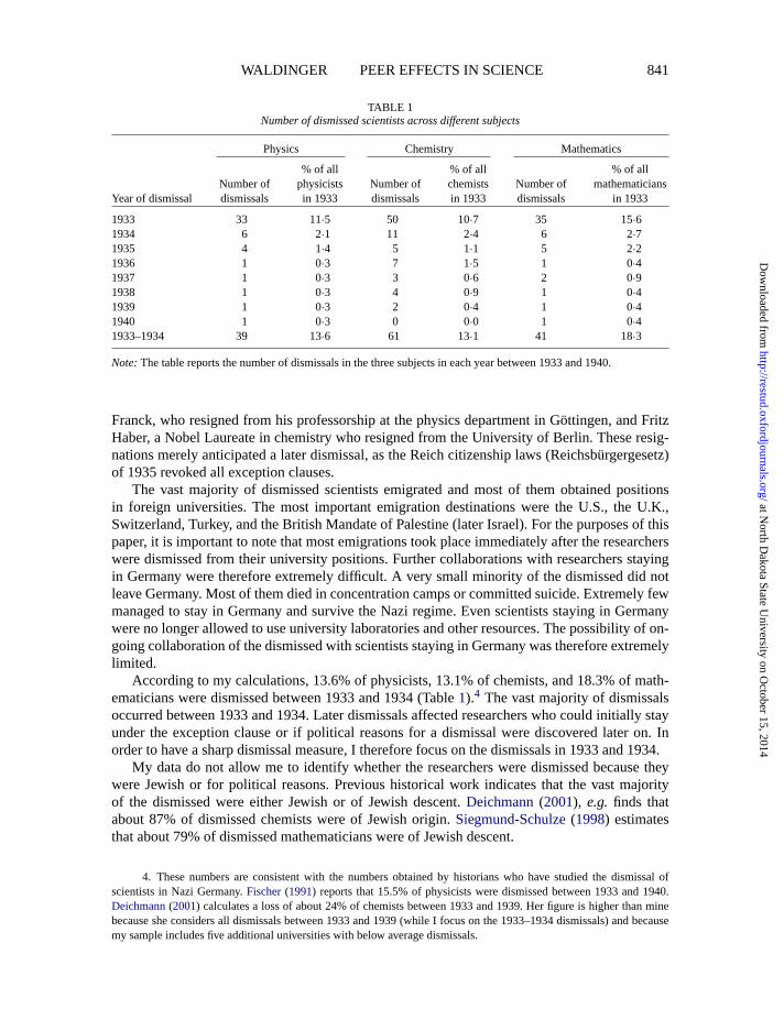
TABLE 1Number of dismissed scientists across differentsubjects

Physics Chemistry Mathematics

% of all % of all % of allNumber of physicists Number of chemists Number of mathematicians

Year of dismissal dismissals in 1933 dismissals in 1933 dismissals in1933

1933 33 11∙5 50 10∙7 35 15∙61934 6 2∙1 11 2∙4 6 2∙71935 4 1∙4 5 1∙1 5 2∙21936 1 0∙3 7 1∙5 1 0∙41937 1 0∙3 3 0∙6 2 0∙91938 1 0∙3 4 0∙9 1 0∙41939 1 0∙3 2 0∙4 1 0∙41940 1 0∙3 0 0∙0 1 0∙41933–1934 39 13∙6 61 13∙1 41 18∙3

Note:Thetable reports the number of dismissals in the three subjects in each year between 1933 and 1940.

Franck,who resigned from his professorship at the physics department in Göttingen, and FritzHaber, a Nobel Laureate in chemistry who resigned from the University of Berlin. These resig-nations merely anticipated a later dismissal, as the Reich citizenship laws (Reichsbürgergesetz)of 1935 revoked all exception clauses.

The vast majority of dismissed scientists emigrated and most of them obtained positionsin foreign universities. The most important emigration destinations were the U.S., the U.K.,Switzerland, Turkey, and the British Mandate of Palestine (later Israel). For the purposes of thispaper, it is important to note that most emigrations took place immediately after the researcherswere dismissed from their university positions. Further collaborations with researchers stayingin Germany were therefore extremely difficult. A very small minority of the dismissed did notleave Germany. Most of them died in concentration camps or committed suicide. Extremely fewmanaged to stay in Germany and survive the Nazi regime. Even scientists staying in Germanywere no longer allowed to use university laboratories and other resources. The possibility of on-going collaboration of the dismissed with scientists staying in Germany was therefore extremelylimited.

According to my calculations, 13.6% of physicists, 13.1% of chemists, and 18.3% of math-ematicians were dismissed between 1933 and 1934 (Table1).4 Thevast majority of dismissalsoccurred between 1933 and 1934. Later dismissals affected researchers who could initially stayunder the exception clause or if political reasons for a dismissal were discovered later on. Inorder to have a sharp dismissal measure, I therefore focus on the dismissals in 1933 and 1934.

My data do not allow me to identify whether the researchers were dismissed because theywere Jewish or for political reasons. Previous historical work indicates that the vast majorityof the dismissed were either Jewish or of Jewish descent.Deichmann(2001),e.g. finds thatabout 87% of dismissed chemists were of Jewish origin.Siegmund-Schulze(1998) estimatesthat about 79% of dismissed mathematicians were of Jewish descent.

4. These numbers are consistent with the numbers obtained by historians who have studied the dismissal ofscientists in Nazi Germany.Fischer(1991) reports that 15.5% of physicists were dismissed between 1933 and 1940.Deichmann(2001) calculates a loss of about 24% of chemists between 1933 and 1939. Her figure is higher than minebecause she considers all dismissals between 1933 and 1939 (while I focus on the 1933–1934 dismissals) and becausemy sample includes five additional universities with below average dismissals.

at North D



Dow

nloaded from


“rdr029” — 2012/4/17 — 12:44 — page 842 — #5


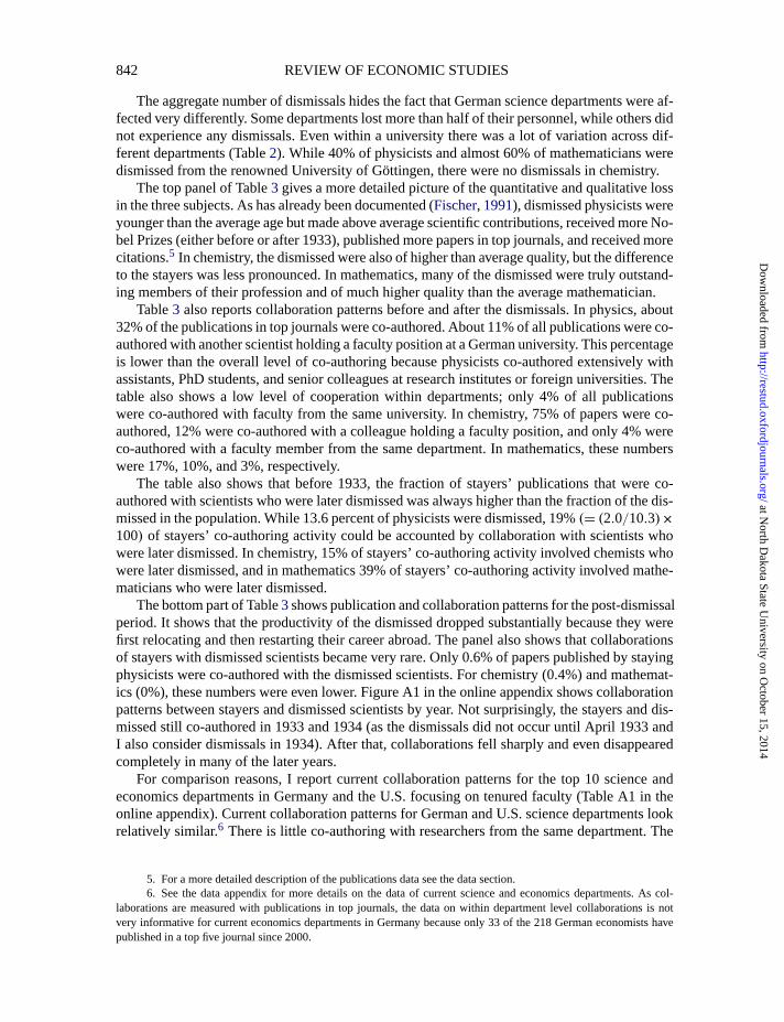
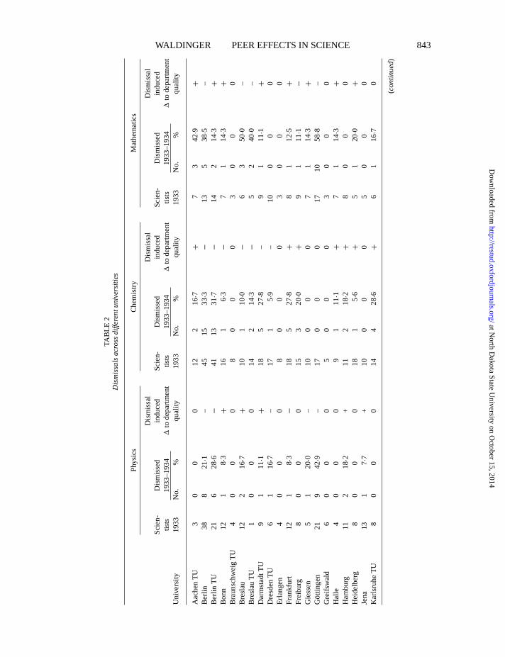
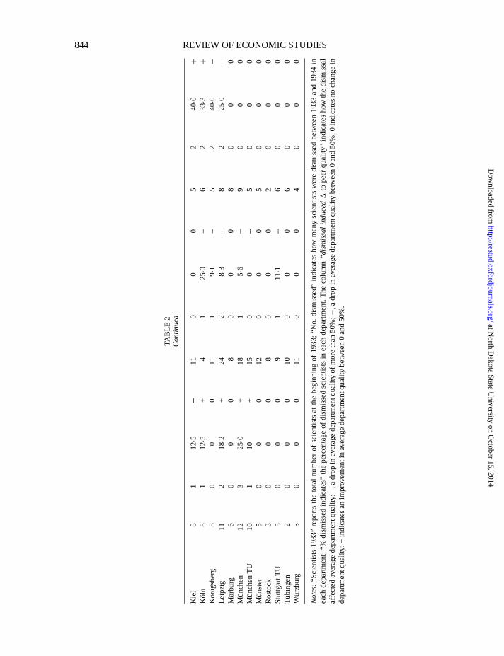
The aggregate number of dismissals hides the fact that German science departments were af-fected very differently. Some departments lost more than half of their personnel, while others didnot experience any dismissals. Even within a university there was a lot of variation across dif-ferent departments (Table2). While 40% of physicists and almost 60% of mathematicians weredismissed from the renowned University of Göttingen, there were no dismissals in chemistry.

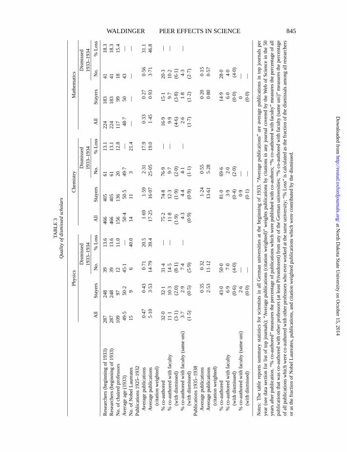
The top panel of Table3 gives a more detailed picture of the quantitative and qualitative lossin the three subjects. As has already been documented (Fischer,1991), dismissed physicists wereyounger than the average age but made above average scientific contributions, received more No-bel Prizes (either before or after 1933), published more papers in top journals, and received morecitations.5 In chemistry, the dismissed were also of higher than average quality, but the differenceto the stayers was less pronounced. In mathematics, many of the dismissed were truly outstand-ing members of their profession and of much higher quality than the average mathematician.

Table3 also reports collaboration patterns before and after the dismissals. In physics, about32% of the publications in top journals were co-authored. About 11% of all publications were co-authored with another scientist holding a faculty position at a German university. This percentageis lower than the overall level of co-authoring because physicists co-authored extensively withassistants, PhD students, and senior colleagues at research institutes or foreign universities. Thetable also shows a low level of cooperation within departments; only 4% of all publicationswere co-authored with faculty from the same university. In chemistry, 75% of papers were co-authored, 12% were co-authored with a colleague holding a faculty position, and only 4% wereco-authored with a faculty member from the same department. In mathematics, these numberswere 17%, 10%, and 3%, respectively.

The table also shows that before 1933, the fraction of stayers’ publications that were co-authored with scientists who were later dismissed was always higher than the fraction of the dis-missed in the population. While 13.6 percent of physicists were dismissed, 19%(= (2.0/10.3)×100)of stayers’ co-authoring activity could be accounted by collaboration with scientists whowere later dismissed. In chemistry, 15% of stayers’ co-authoring activity involved chemists whowere later dismissed, and in mathematics 39% of stayers’ co-authoring activity involved mathe-maticians who were later dismissed.

The bottom part of Table3shows publication and collaboration patterns for the post-dismissalperiod. It shows that the productivity of the dismissed dropped substantially because they werefirst relocating and then restarting their career abroad. The panel also shows that collaborationsof stayers with dismissed scientists became very rare. Only 0.6% of papers published by stayingphysicists were co-authored with the dismissed scientists. For chemistry (0.4%) and mathemat-ics (0%), these numbers were even lower. Figure A1 in the online appendix shows collaborationpatterns between stayers and dismissed scientists by year. Not surprisingly, the stayers and dis-missed still co-authored in 1933 and 1934 (as the dismissals did not occur until April 1933 andI also consider dismissals in 1934). After that, collaborations fell sharply and even disappearedcompletely in many of the later years.

For comparison reasons, I report current collaboration patterns for the top 10 science andeconomics departments in Germany and the U.S. focusing on tenured faculty (Table A1 in theonline appendix). Current collaboration patterns for German and U.S. science departments lookrelatively similar.6 Thereis little co-authoring with researchers from the same department. The

5. For a more detailed description of the publications data see the data section.6. See the data appendix for more details on the data of current science and economics departments. As col-

laborations are measured with publications in top journals, the data on within department level collaborations is notvery informative for current economics departments in Germany because only 33 of the 218 German economists havepublished in a top five journal since 2000.

at North D



Dow

nloaded from


“rdr029” — 2012/4/17 — 12:44 — page 843 — #6


TAB

LE2

Dis

mis

sals

acr

oss

diff

ere

ntu

niv

er

sitie

s

Phy

sics

Che

mis

try

Mat

hem

atic

s

Dis

mis

sal

Dis

mis

sal

Dis

mis

sal

Sci

en-

Dis

mis

sed

indu

ced

Sci

en-

Dis

mis

sed

indu

ced

Sci

en-

Dis

mis

sed

indu

ced

tists

1933

–193

41

tode

part

men

ttis

ts19

33–1

934

1to

depa

rtm

ent

tists

1933

–193

41

tode

part

men

tU

nive

rsity

1933

No.

%qu

ality

1933

No.

%qu

ality

1933

No.

%qu

ality

Aac

hen T

U3

00

012

216

∙7+

73

42∙9

+B

erlin

388

21∙1

–45

1533

∙3−

135

38∙5

–B

erlin

TU

216

28∙6

−41

1331

∙7−

142

14∙3

+B

onn

121

8∙3

+16

16∙

3−

71

14∙3

+B

raun

schw

eig

TU

40

00

80

00

30

00

Bre

slau

122

16∙7

+10

110

∙0−

63

50∙0

–B

resl

auT

U1

00

014

214

∙3−

52

40∙0

–D

arm

stad

tTU

91

11∙1

+18

527

∙8–

91

11∙1

+D

resd

enT

U6

116

∙7–

171

5∙9

–10

00

0E

rlang

en4

00

08

00

03

00

0F

rank

furt

121

8∙3

−18

527

∙8+

81

12∙5

+F

reib

urg

80

00

153

20∙0

+9

111

∙1−

Gie

ssen

51

20∙0

–10

00

07

114

∙3+

Göt

tinge

n21

942

∙9–

170

00

1710

58∙8

–G

reifs

wal

d6

00

05

00

03

00

0H

alle

40

00

91

11∙1

+7

114

∙3+

Ham

burg

112

18∙2

+11

218

∙2+

80

00

Hei

delb

erg

80

00

181

5∙6

+5

120

∙0+

Jena

131

7∙7

+10

00

05

00

0K

arls

ruhe

TU

80

00

144

28∙6

+6

116

∙70

(co

ntin

ue

d)

at North D



Dow

nloaded from


“rdr029” — 2012/4/17 — 12:44 — page 844 — #7


TAB

LE2

Co

ntin

ue

d

Kie

l8

112

∙5−

110

00

52

40∙0

+K

öln

81

12∙5

+4

125

∙0–

62

33∙3

+K

önig

sber

g8

00

011

19∙

1–

52

40∙0

−Le

ipzi

g11

218

∙2+

242

8∙3

−8

225

∙0−

Mar

burg

60

00

80

00

80

00

Mün

chen

123

25∙0

+18

15∙

6−

90

00

Mün

chen

TU

101

10+

150

0+

50

00

Mün

ster

50

00

120

00

50

00

Ros

tock

30

00

80

00

20

00

Stu

ttgar

tTU

50

00

91

11∙1

+6

00

0T

übin

gen

20

00

100

00

60

00

Wür

zbur

g3

00

011

00

04

00

0

No

tes:

“Sci

entis

ts19

33”

repo

rts

the

tota

lnum

ber

ofsc

ient

ists

atth

ebe

ginn

ing

of19

33;

“No.

dism

isse

d”in

dica

tes

how

man

ysc

ient

ists

wer

edi

smis

sed

betw

een

1933

and

1934

inea

chde

part

men

t;“%

dism

isse

din

dica

tes”

the

perc

enta

geof

dism

isse

dsc

ient

ists

inea

chde

part

men

t.T

heco

lum

n“d

ism

issa

lin

du

ced1

tope

erqu

ality

”in

dica

tes

how

the

dism

issa

laf

fect

edav

erag

ede

part

men

tqua

lity:

–,a

drop

inav

erag

ede

part

men

tqua

lity

ofm

ore

than

50%

;−

,adr

opin

aver

age

depa

rtm

entq

ualit

ybe

twee

n0

and

50%

;0in

dica

tes

noch

ange

inde

part

men

tqua

lity;

+in

dica

tes

anim

prov

emen

tin

aver

age

depa

rtm

entq

ualit

ybe

twee

n0

and

50%

.

at North D



Dow

nloaded from


“rdr029” — 2012/4/17 — 12:44 — page 845 — #8


TAB

LE3

Qu

alit

yo

fdis

mis

sed

sch

ola

rs

Phy

sics

Che

mis

try

Mat

hem

atic

s

Dis

mis

sed

Dis

mis

sed

Dis

mis

sed

1933

–193

419

33–1

934

1933

–193

4

All

Sta

yers

No.

%Lo

ssA

llS

taye

rsN

o.%

Loss

All

Sta

yers

No.

%Lo

ss

Res

earc

hers(

begi

nnin

gof

1933

)28

724

839

13.6

466

405

6113

.122

418

341

18.3

Res

earc

hers

(beg

inni

ngof

1933

)28

724

839

13.6

466

405

6113

.122

418

341

18.3

No.

ofch

aire

dpr

ofes

sors

109

9712

11.0

156

136

2012

.811

799

1815

.4A

vera

geag

e(1

933)

49∙5

50∙2

45∙1

—50

∙450

∙549

∙7—

48∙7

5043

—N

o.of

Nob

elLa

urea

tes

159

640

.014

113

21.4

——

——

Pub

licat

ions

1925

–193

2A

vera

gepu

blic

atio

ns0∙4

70∙

430∙

7120

.51∙6

91∙

592∙

3117

.90∙3

30∙

270∙

5631

.1A

vera

gepu

blic

atio

ns5∙1

03∙

5314

∙79

39.4

17∙2

516

∙07

25∙0

519

.01∙4

50∙

933∙

7146

.8(c

itatio

nw

eigh

ted)

%co

-aut

hore

d32

∙032

∙131

∙4—

75∙2

74∙8

76∙9

—16

∙915

∙120

∙3—

%co

-aut

hore

dw

ithfa

culty

11∙1

10∙3

14∙5

—11

∙812

∙39∙

7—

9∙9

9∙7

10∙2

—(w

ithdi

smis

sed)

(3∙1

)(2

.0)

(8∙1

)(1

∙9)

(1∙9

)(2

∙0)

(4∙6

)(3

∙8)

(6∙1

)%

co-a

utho

red

with

facu

lty(s

ame

uni)

3∙7

2∙9

7∙4

—4∙

34∙

44∙

1—

2∙6

1∙8

4∙3

—(w

ithdi

smis

sed)

(1∙5

)(0

∙5)

(5∙9

)(0

∙9)

(0∙9

)(1

∙1)

(1∙7

)(1

∙2)

(2∙7

)P

ublic

atio

ns19

35–1

938

Ave

rage

publ

icat

ions

0∙35

0∙32

1∙24

0∙55

0∙20

0∙15

Ave

rage

publ

icat

ions

2∙53

11∙1

213

∙61

5∙28

0∙80

0∙57

(cita

tion

wei

ghte

d)%

co-a

utho

red

43∙0

50∙0

81∙0

69∙6

14∙9

28∙0

%co

-aut

hore

dw

ithfa

culty

6∙9

7∙0

3∙9

2∙0

6∙0

4∙0

(with

dism

isse

d)(0

∙6)

(4∙0

)(0

∙4)

(2∙0

)(0

∙0)

(4∙0

)%

co-a

utho

red

with

facu

lty(s

ame

uni)

2∙6

—0∙

9—

0—

(with

dism

isse

d)(0

∙0)

—(0

∙1)

—(0

∙0)

—

No

tes:

The

tabl

ere

port

ssu

mm

ary

stat

istic

sfo

rsc

ient

ists

inal

lG

erm

anun

iver

sitie

sat

the

begi

nnin

gof

1933

.“A

vera

gepu

blic

atio

ns”

are

aver

age

publ

icat

ions

into

pjo

urna

lspe

rye

ar(s

eeda

tase

ctio

nfo

rlis

tof

top

jour

nals

);“A

vera

gepu

blic

atio

ns(c

itatio

nw

eigh

ted)

”w

eigh

tspu

blic

atio

nsby

cita

tions

inan

yjo

urna

lcov

ered

byth

eW

ebof

Sci

ence

inth

e50

year

saf

ter

publ

icat

ion.

“%co

-aut

hore

d”m

easu

res

the

perc

enta

geof

publ

icat

ions

whi

chw

ere

publ

ishe

dw

ithco

-aut

hors

;“%

co-a

utho

red

with

facu

lty”

mea

sure

sth

epe

rcen

tage

ofal

lpu

blic

atio

nsth

atw

asco

-aut

hore

dw

ithot

her

prof

esso

rs(a

tlea

stP

rivat

doze

nt)

from

any

ofth

eG

erm

anun

iver

sitie

s;“%

co-a

utho

red

with

facu

lty(s

ame

uni)”

mea

sure

sth

epe

rcen

tage

ofal

lpub

licat

ions

whi

chw

ere

co-a

utho

red

with

othe

rpr

ofes

sors

who

ever

wor

ked

atth

esa

me

univ

ersi

ty;“

%Lo

ss”

isca

lcul

ated

asth

efr

actio

nof

the

dism

issa

lsam

ong

allr

esea

rche

rsor

asth

efr

actio

nof

Nob

elLa

urea

tes,

publ

icat

ions

,and

cita

tion

wei

ghte

dpu

blic

atio

nsw

hich

wer

eco

ntrib

uted

byth

edi

smis

sed.

at North D



Dow

nloaded from


“rdr029” — 2012/4/17 — 12:44 — page 846 — #9


big exception is physics with a high level of collaboration within departments. This is mostlydriven, however, by physicists conducting research involving particle accelerators; a technologythat was invented by E. Lawrence in Berkeley in 1930 and became first available in Germanyin 1944, and thus after the time period analysed in this paper. The publications involving resultsfrom particle accelerators usually list hundreds of authors (often more than 500, one article inthe Physical Review Letters even has 744 authors). For physicists working with particle acceler-ators, co-authoring does therefore not seem a very good measure for close collaboration. If oneexcludes these physicists from the analysis (about 15% of physicists overall), current collabora-tion patterns are more similar to the historical data for physicists as well.

3. CONSTRUCTION OF A PANEL DATA SET OF GERMAN SCIENTISTS

3.1. Data on dismissed scholars

I obtain data on dismissals from a number of historical sources. The main source is theList of Displaced German Scholars (Notgemeinschaft Deutscher Wissenschaftler Ausland, 1937)from which I extract all dismissed physicists, chemists, and mathematicians. The list was com-piled by the relief organization “Emergency Alliance of German Scholars Abroad”, which sup-ported dismissed scholars in finding positions in foreign universities. It contains about 1650names of dismissed university researchers from all subjects. Online appendix 2 shows a sam-ple page from the physics section of the list. The page shows four physicists who had alreadyreceived the Nobel Prize or were to receive it in later years (Figure A6).

For various reasons,e.g.if the dismissed died before the List of Displaced German Scholarswas compiled, a small number of dismissed researchers did not appear in the list. To get amore complete measure of all dismissals I complement the data on dismissals with informationfrom secondary sources (Biographisches Handbuch, 1983,Kroener(1983);Beyerchen, 1977;Siegmund-Schulze, 1998;Deichmann,2001).7 Onlineappendix 2 contains more detail on dataconstruction and the secondary sources.

3.2. Data on all scientists at German universities between 1925 and 1938

To investigate the impact of the dismissals on scientists who stayed in Germany, I obtain dataon all scientists in German universities from 1925 to 1938. The data originate from historicalUniversity Calendars (see online appendix 2 for details) from which I compile an annual ros-ter of scientists in all physics, chemistry, and mathematics departments from winter semester1924/1925 (lasting from November 1924 until April 1925) to winter semester 1937/1938.8 Thedatacontain all scientists who were at least “Privatdozent”. That is the first university position aresearcher could obtain after the “venia legendi” and would allow the researcher to give lecturesat German universities.

In some specifications, I use the scientists’ specialization to identify their relevant peer group.The data on specializations come from seven volumes of “Kürschners Deutscher Gelehrten-Kalender”. The books are listings of German researchers compiled at irregular intervals since1925. The Gelehrtenkalender contains about 90% of scientists in my sample. For the remain-ing 10%, I conduct an internet search to find the scientists’ specialization. Overall, I obtain

7. Slightly less than 20% of 1933 to 1934 dismissals only appear in the additional sources but not in the “List ofDisplaced German Scholars”.

8. Data for the technical universities were only published from winter semester 1927/1928 onwards.

at North D



Dow

nloaded from


“rdr029” — 2012/4/17 — 12:44 — page 847 — #10


information on the specialization for 98% of the scientists.9 Table A2 in online appendix 1 givesan overview of all specializations and the fraction of scientists in each of them.

3.3. Publication data

To measure the productivity of scientists, I construct a data set containing the publications ofeach researcher in the top academic journals of the time. In the period under consideration, mostGerman scientists published in German journals. German journals were of very high qualitybecause many of the German physicists, chemists, and mathematicians were among the leadersin their profession. This is especially true for the time before the dismissals, as is exemplified bythe following quote: “Before the advent of the Nazis the German physics journals (Zeitschrift fürPhysik, Annalen der Physik, Physikalische Zeitschrift) had always served as the central organsof world science in this domain [. . . ]. In 1930, approximately 700 scientific papers were printedin its [the Zeitschrift für Physik’s] seven volumes of which 280 were by foreign scientists”(American Association for the Advancement of Science, 1941). Historical research indicatesthat the journals considered in the analysis did not change substantially between 1933 and 1938(Simonsohn,2007). It is important to note that the identification strategy outlined below relies onchanges in publications of researchers in German departments that were differentially affectedby the dismissals. A decline in the quality of the considered journals would therefore not affectmy results, as all regressions are estimated including year fixed effects.

The top publications measure is based on articles contained in the online database “ISI Webof Science”. The database is provided by Thomson Scientific and contains all contributions ina large number of science journals. In 2004, the database was extended to include articles injournals published between 1900 and 1945. The journals included in this backward extensionwere all journals that had published the most relevant articles in the years 1900 to 1945. Thepublication measure used in this paper therefore measures publications in the top journals of thetime.

I extract all German-speaking general science, physics, chemistry, and mathematics journalsthat are included in the database for the time period 1925–1938. Furthermore, I add the leadinggeneral science journals that were not published in Germany, namelyNature, Science, andtheProceedings of the Royal Society of London. I also include four non-German top specializedjournals that were suggested by historians of science as journals of some importance for theGerman scientific community (see online appendix 2 for details). Online appendix Table A3lists all journals used in the analysis.

For each researcher, I calculate two yearly productivity measures. The first measure is equalto the sum of publications in top journals in a given year. In order to quantify an article’s quality, Ialso construct a second measure that accounts for the number of times the article was cited in anyjournal included in the Web of Science in the first 50 years after its publication. This includescitations in journals that are not in my list of journals but that appear in the Web of Science.As a result, this measure includes citations from the entire international scientific community.It is therefore less heavily based on German science. I call this measure “citation weightedpublications” and it is defined as the sum of citations to all articles published in a certain year.

Online appendix Table A4 lists the top 20 researchers for each subject according to the ci-tation weighted publications measure. It is reassuring to realize that the vast majority of thesetop 20 researchers are very well known in the scientific community. Economists will find itinteresting that Johann von Neumann who emigrated to the Institute of Advanced Studies in

9. Some researchers name more than one specialization. Physicists and chemists therefore have up to twospecializations and mathematicians up to four.

at North D



Dow

nloaded from


“rdr029” — 2012/4/17 — 12:44 — page 848 — #11


Princeton was the most cited mathematician. The large number of Nobel Laureates among thetop 20 researchers indicates that citation weighted publications are a good measure of a scholar’sproductivity.

4. IDENTIFICATION

4.1. Estimating peer effects

Using this panel data set, I estimate peer effects among scientists. The collaboration of re-searchers can take different levels of intensity. A very direct way of peer interaction is the col-laboration on joint research projects involving joint publication of results. In many cases, how-ever, peer interactions are more subtle. Scientists discuss research ideas and comment on eachother’s work without co-publishing. Yet another way in which peers may affect a researcher’sproductivity is through peer pressure. Furthermore, peers may attract more research funding tothe department or have better contacts to influential members of the profession. In this paper, Iestimate the sum of all aforementioned peer effects.

The standard approach when estimating peer effects consists of regressing an individual’sproductivity on the average productivity of his peers. The productivity of academic researchers,however, is not only affected by the average quality of peers but also by the number of peersthey can interact with.

As university departments differ substantially in quality and size, it is important to distin-guish these two dimensions of peer effects among scientists. I therefore propose the followingregression which will be estimated for all scientists staying in Germany (in the following I willrefer to them as “stayers”):

# Publicationsi ut = β1 +β2(PeerQuality)ut +β3(# of Peers)ut +β4AgeDummiesi ut

+β5YearF Et +β6IndividualF Ei + εi ut. (1)

I regress the number of publications of scientisti in university u and yeart on measures ofhis peer group and other controls. The regressions are estimated separately for physics, chem-istry, and mathematics because the subjects under consideration have different publication andcollaboration patterns. Peer quality is calculated as the mean of the average productivity of aresearcher’s peers.10 Over time changes in average peer quality only occur if the composition ofthe department changes. Yearly fluctuations in publications of the same set of peers do thereforenot affect peer quality. The underlying assumption is that Albert Einstein always had the sameeffect on his peers independently of how much he published in a given year.

It is likely that the effect of peers is only measurable after a certain time lag. Peers influencethe creation of new ideas and papers before the actual date of publication. Another delay iscaused by publication lags. Science research is published much faster than research in othersubjects like economics. Anecdotal evidence suggests that the effect of peers should be measuredwith a lag of about 1 year. Co-authoring of scientists staying in Germany with colleagues whowere dismissed in 1933 and 1934 allow the investigation of likely lags of peer interactions.Figure A1 in online appendix 1 reports the fraction of papers that stayers co-authored with

10. To measure average peer quality, I use the department mean of individual productivities calculated between1925 and 1938. An alternative way of measuring average peer quality uses only pre-dismissal years. This measure,however, is not defined for researchers coming into the sample after 1933. I therefore present results using the firstmeasure. Using the alternative measure does not affect my findings.

at North D



Dow

nloaded from


“rdr029” — 2012/4/17 — 12:44 — page 849 — #12


dismissed scientists. As chemists not only co-published a larger amount of their papers but alsopublished more papers on average, the data for chemistry are the least noisy. The number ofstayers’ publications with the dismissed scientists plummeted in 1935, exactly the year after thedismissals considered in this paper. I therefore use 1 year lag for the peer group variables whenestimating equation (1). Using different lags does not affect the results.

The regression also includes a full set of 5-year age group dummies to control for life cyclechanges in productivity. Year fixed effects control for yearly fluctuations in publications thataffect all researchers in the same way. To control for differences in a researcher’s talent, I addindividual fixed effects to all specifications. In some robustness checks, I also add universityfixed effects to control for university-specific factors affecting a researcher’s productivity. Thesecan be separately identified because some scientists change universities.

4.2. Using the dismissals as instruments for the number and quality of peers

Estimating equation (1) using OLS would lead to biased estimates ofβ2 andβ3. An impor-tant problem is caused by selection. Selection not only occurs because scientists self-select intodepartments with peers of similar quality but also because departments appoint professors ofsimilar productivity. Omitted variables, such as the (unobserved) construction of a new labora-tory, may further complicate the estimation of peer effects. Furthermore, measuring peer qualitywith error could bias the regression estimates.11

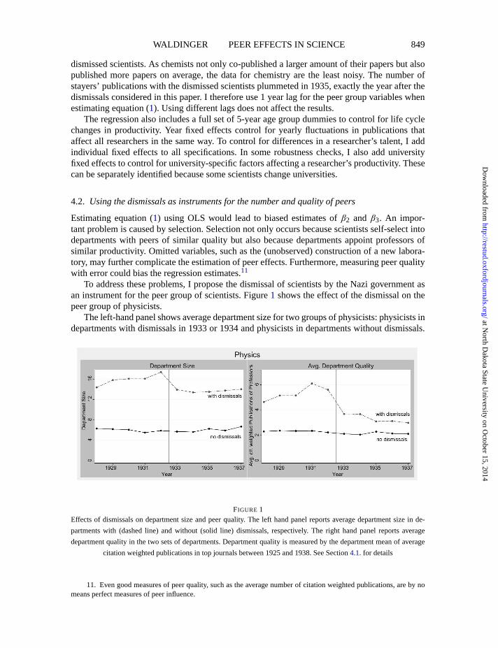
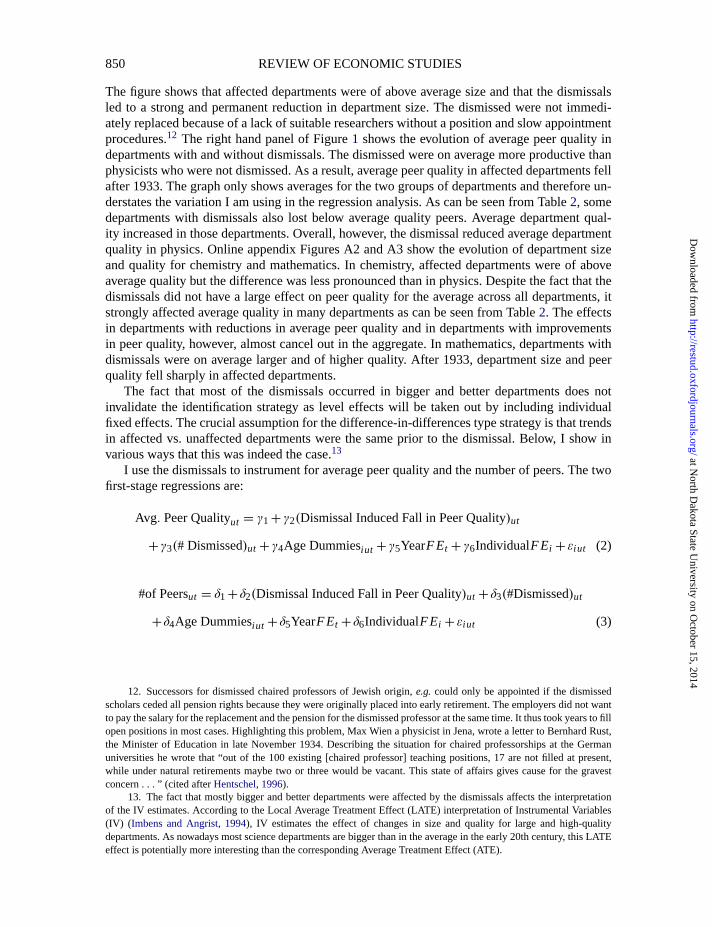
To address these problems, I propose the dismissal of scientists by the Nazi government asan instrument for the peer group of scientists. Figure1 shows the effect of the dismissal on thepeer group of physicists.

The left-hand panel shows average department size for two groups of physicists: physicists indepartments with dismissals in 1933 or 1934 and physicists in departments without dismissals.

FIGURE 1Effects of dismissals on department size and peer quality. The left hand panel reports average department size in de-

partments with (dashed line) and without (solid line) dismissals, respectively. The right hand panel reports average

department quality in the two sets of departments. Department quality is measured by the department mean of average

citation weighted publications in top journals between 1925 and 1938. See Section4.1. for details

11. Even good measures of peer quality, such as the average number of citation weighted publications, are by nomeans perfect measures of peer influence.

at North D



Dow

nloaded from


“rdr029” — 2012/4/17 — 12:44 — page 850 — #13


The figure shows that affected departments were of above average size and that the dismissalsled to a strong and permanent reduction in department size. The dismissed were not immedi-ately replaced because of a lack of suitable researchers without a position and slow appointmentprocedures.12 The right hand panel of Figure1 shows the evolution of average peer quality indepartments with and without dismissals. The dismissed were on average more productive thanphysicists who were not dismissed. As a result, average peer quality in affected departments fellafter 1933. The graph only shows averages for the two groups of departments and therefore un-derstates the variation I am using in the regression analysis. As can be seen from Table2, somedepartments with dismissals also lost below average quality peers. Average department qual-ity increased in those departments. Overall, however, the dismissal reduced average departmentquality in physics. Online appendix Figures A2 and A3 show the evolution of department sizeand quality for chemistry and mathematics. In chemistry, affected departments were of aboveaverage quality but the difference was less pronounced than in physics. Despite the fact that thedismissals did not have a large effect on peer quality for the average across all departments, itstrongly affected average quality in many departments as can be seen from Table2. The effectsin departments with reductions in average peer quality and in departments with improvementsin peer quality, however, almost cancel out in the aggregate. In mathematics, departments withdismissals were on average larger and of higher quality. After 1933, department size and peerquality fell sharply in affected departments.

The fact that most of the dismissals occurred in bigger and better departments does notinvalidate the identification strategy as level effects will be taken out by including individualfixed effects. The crucial assumption for the difference-in-differences type strategy is that trendsin affected vs. unaffected departments were the same prior to the dismissal. Below, I show invarious ways that this was indeed the case.13

I use the dismissals to instrument for average peer quality and the number of peers. The twofirst-stage regressions are:

Avg. Peer Qualityut = γ1 +γ2(DismissalInduced Fall in Peer Quality)ut

+γ3(# Dismissed)ut +γ4AgeDummiesi ut +γ5YearF Et +γ6IndividualF Ei + εi ut (2)

#of Peersut = δ1 + δ2(DismissalInduced Fall in Peer Quality)ut + δ3(#Dismissed)ut

+δ4AgeDummiesi ut + δ5YearF Et + δ6IndividualF Ei + εi ut (3)

12. Successors for dismissed chaired professors of Jewish origin,e.g.could only be appointed if the dismissedscholars ceded all pension rights because they were originally placed into early retirement. The employers did not wantto pay the salary for the replacement and the pension for the dismissed professor at the same time. It thus took years to fillopen positions in most cases. Highlighting this problem, Max Wien a physicist in Jena, wrote a letter to Bernhard Rust,the Minister of Education in late November 1934. Describing the situation for chaired professorships at the Germanuniversities he wrote that “out of the 100 existing [chaired professor] teaching positions, 17 are not filled at present,while under natural retirements maybe two or three would be vacant. This state of affairs gives cause for the gravestconcern . . . ” (cited afterHentschel,1996).

13. The fact that mostly bigger and better departments were affected by the dismissals affects the interpretationof the IV estimates. According to the Local Average Treatment Effect (LATE) interpretation of Instrumental Variables(IV) (Imbens and Angrist, 1994), IV estimates the effect of changes in size and quality for large and high-qualitydepartments. As nowadays most science departments are bigger than in the average in the early 20th century, this LATEeffect is potentially more interesting than the corresponding Average Treatment Effect (ATE).

at North D



Dow

nloaded from


“rdr029” — 2012/4/17 — 12:44 — page 851 — #14


Equation (2) is the first-stage regression for average peer quality. The crucial instrumentfor average peer quality is called “Dismissal Induced Fall in Peer Quality”. It measures howmuch average peer quality fell because of the dismissals. The variable is zero until 1933 in alldepartments. After 1933, it is defined as follows:

Dismissal Induced Fall in Peer Quality= (Avg. Peer Quality before1933)

−(Avg. Peer Quality before 1933|stayer)

After 1933, “Dismissal Induced Fall in Peer Quality” is positive for scientists in departmentswith dismissals of above average department quality. The variable remains zero for researchersin departments without dismissals or for scientists who lost peers whose quality was below thedepartment average.14 The instrument is based on changes in peer quality measured by 1925–1932 productivity measures. Using quality measures after 1933 in the construction of the instru-mental variable would be problematic because post-1933 productivity may be affected by thedismissals.

The second instrument is the number of dismissals in a given department. The variable iszero until 1933 and equal to the number of dismissals thereafter.15

Thedismissals may have caused some scientists to change university after 1933. The changeis likely to be endogenous and thus have a direct effect on researchers’ productivity. I thereforeassign each scientist the dismissal variables for the department he attended at the beginning of1933. As the dismissal effect is likely to be correlated for all stayers in a department, I clusterstandard errors at the university level.

5. THE EFFECT OF DISMISSALS ON SCIENTISTS WHO REMAINED IN GERMANY

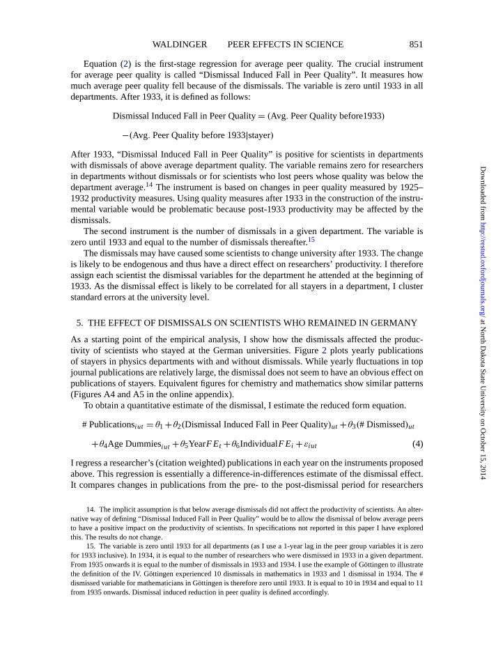
As a starting point of the empirical analysis, I show how the dismissals affected the produc-tivity of scientists who stayed at the German universities. Figure2 plots yearly publicationsof stayers in physics departments with and without dismissals. While yearly fluctuations in topjournal publications are relatively large, the dismissal does not seem to have an obvious effect onpublications of stayers. Equivalent figures for chemistry and mathematics show similar patterns(Figures A4 and A5 in the online appendix).

To obtain a quantitative estimate of the dismissal, I estimate the reduced form equation.

# Publicationsi ut = θ1 + θ2(DismissalInduced Fall in Peer Quality)ut + θ3(# Dismissed)ut

+θ4AgeDummiesi ut + θ5YearF Et + θ6IndividualF Ei + εi ut (4)

I regress a researcher’s (citation weighted) publications in each year on the instruments proposedabove. This regression is essentially a difference-in-differences estimate of the dismissal effect.It compares changes in publications from the pre- to the post-dismissal period for researchers

14. The implicit assumption is that below average dismissals did not affect the productivity of scientists. An alter-native way of defining “Dismissal Induced Fall in Peer Quality” would be to allow the dismissal of below average peersto have a positive impact on the productivity of scientists. In specifications not reported in this paper I have exploredthis. The results do not change.

15. The variable is zero until 1933 for all departments (as I use a 1-year lag in the peer group variables it is zerofor 1933 inclusive). In 1934, it is equal to the number of researchers who were dismissed in 1933 in a given department.From 1935 onwards it is equal to the number of dismissals in 1933 and 1934. I use the example of Göttingen to illustratethe definition of the IV. Göttingen experienced 10 dismissals in mathematics in 1933 and 1 dismissal in 1934. The #dismissed variable for mathematicians in Göttingen is therefore zero until 1933. It is equal to 10 in 1934 and equal to 11from 1935 onwards. Dismissal induced reduction in peer quality is defined accordingly.

at North D



Dow

nloaded from


“rdr029” — 2012/4/17 — 12:44 — page 852 — #15


FIGURE 2Effect of dismissal on stayers. The average yearly publications in top journals of stayers in affected (dashed line) and

unaffected (solid line) departments, respectively, are given

in affected departments to the change between the two periods for unaffected researchers. Ifthe dismissals had a negative effect on the productivity of stayers, one would expect negativecoefficients on the dismissal variables.

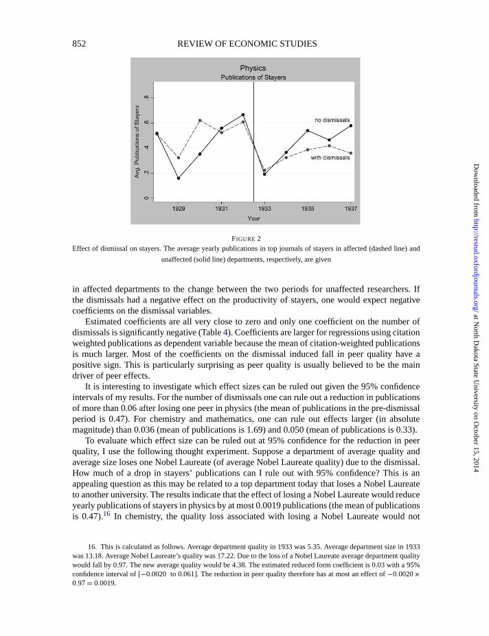
Estimated coefficients are all very close to zero and only one coefficient on the number ofdismissals is significantly negative (Table4). Coefficients are larger for regressions using citationweighted publications as dependent variable because the mean of citation-weighted publicationsis much larger. Most of the coefficients on the dismissal induced fall in peer quality have apositive sign. This is particularly surprising as peer quality is usually believed to be the maindriver of peer effects.

It is interesting to investigate which effect sizes can be ruled out given the 95% confidenceintervals of my results. For the number of dismissals one can rule out a reduction in publicationsof more than 0.06 after losing one peer in physics (the mean of publications in the pre-dismissalperiod is 0.47). For chemistry and mathematics, one can rule out effects larger (in absolutemagnitude) than 0.036 (mean of publications is 1.69) and 0.050 (mean of publications is 0.33).

To evaluate which effect size can be ruled out at 95% confidence for the reduction in peerquality, I use the following thought experiment. Suppose a department of average quality andaverage size loses one Nobel Laureate (of average Nobel Laureate quality) due to the dismissal.How much of a drop in stayers’ publications can I rule out with 95% confidence? This is anappealing question as this may be related to a top department today that loses a Nobel Laureateto another university. The results indicate that the effect of losing a Nobel Laureate would reduceyearly publications of stayers in physics by at most 0.0019 publications (the mean of publicationsis 0.47).16 In chemistry, the quality loss associated with losing a Nobel Laureate would not

16. This is calculated as follows. Average department quality in 1933 was 5.35. Average department size in 1933was 13.18. Average Nobel Laureate’s quality was 17.22. Due to the loss of a Nobel Laureate average department qualitywould fall by 0.97. The new average quality would be 4.38. The estimated reduced form coefficient is 0.03 with a 95%confidence interval of [−0.0020 to 0.061]. The reduction in peer quality therefore has at most an effect of−0.0020×0.97= 0.0019.

at North D



Dow

nloaded from


“rdr029” — 2012/4/17 — 12:44 — page 853 — #16


TABLE 4Reduced form (Department level peers)

(1) (2) (3) (4) (5) (6)


Cit. weighted Cit. weighted Cit. weightedDependent variable Publications publications Publications publications Publicationspublications

Dismissalinduced fall 0∙029 0∙312 0∙012 0∙383 0∙022 −0∙464in peer quality (0∙015) (0∙235) (0∙015) (0∙303) (0∙031) (0∙337)

Number dismissed −0∙021 −0∙017 −0∙018 −0∙130 −0∙018 −0∙016(0∙017) (0∙302) (0∙009)∗ (0∙222) (0∙015) (0∙167)

Age dummies Yes Yes Yes Yes Yes YesYear dummies Yes Yes Yes Yes Yes YesIndividual FE Yes Yes Yes Yes Yes Yes

Observations 2261 2261 3584 3584 1538 1538No. of researchers 258 258 413 413 183 183R-squared 0∙39 0∙25 0∙67 0∙54 0∙32 0∙20

Notes:**Significant at 1% level; *significant at 5% level (All standard errors clustered at university level).The dependent variable “Publications” is the sum of a scientist’s publications in top journals in a given year. The al-ternative dependent variable “Cit. weighted publications” is the sum of subsequent citations (in the first 50 years afterpublication) to articles published in top journals by a scientist in a given year. Explanatory variables are defined asfollows. “Dismissal induced fall in peer quality” is 0 for all scientists until 1933. In 1934, it is equal to (Avg. qualityof peers in department before dismissal)− (Avg. quality of peers| not dismissed in 1933) if this number> 0. From1935 onwards it is equal to (Avg. quality of peers in department before dismissal)− (Avg. quality of peers|not dis-missed between 1933 and 1934) if this number is> 0. The variable remains 0 for all other scientists. For scientists indepartments with above average quality dismissals, “Dismissal induced Fall in peer quality” is therefore positive after1933. “Number dismissed” is equal to 0 for all scientists until 1933. In 1934, it is equal to the number of dismissals in1933 in a scientist’s department. From 1935 onwards it is equal to the number of dismissals between 1933 and 1934 ina scientist’s department.

reducepublications by more than 0.031 (the mean of publications is 1.69). In mathematics, onecan rule out a fall in publications of 0.048 for losing a top 20 mathematician, as there is no Nobelprize in mathematics (the mean of publications is 0.33).

Publications and citation-weighted publications are count data with a relatively large propor-tion of zeros and can never be negative. Instead of OLS, one may therefore prefer to estimate thereduced form using a model that specifically addresses the nature of the data. Table A5 in theonline appendix reports Poisson regressions of the reduced form. The results are very similar.17

An important assumption for using the dismissals to identify peer effects is that publicationtrends of stayers in affected and unaffected departments would have followed the same trend inthe absence of the dismissals. To investigate this identification assumption, I therefore estimatea placebo experiment using the pre-dismissal period, only, and moving the dismissal from 1933to 1930. The results reported in online appendix Table A6 indicate that stayers in departmentswith dismissals did not follow different productivity trends before 1933.

17. As Santos Silva and Tenreyro(2010) described, including a fixed effect for a scientist who never publishesleads to convergence problems as the (pseudo) maximum likelihood does not exist in this case. Standard regressionpackages do not address this problem and will therefore lead to non-convergence of the estimator. I therefore use theppml command as suggested bySantos Silva and Tenreyro(2011).

at North D



Dow

nloaded from


“rdr029” — 2012/4/17 — 12:44 — page 854 — #17


6. USING THE DISMISSALS TO IDENTIFY LOCALIZED PEEREFFECTS IN SCIENCE

6.1. Department level peer effects

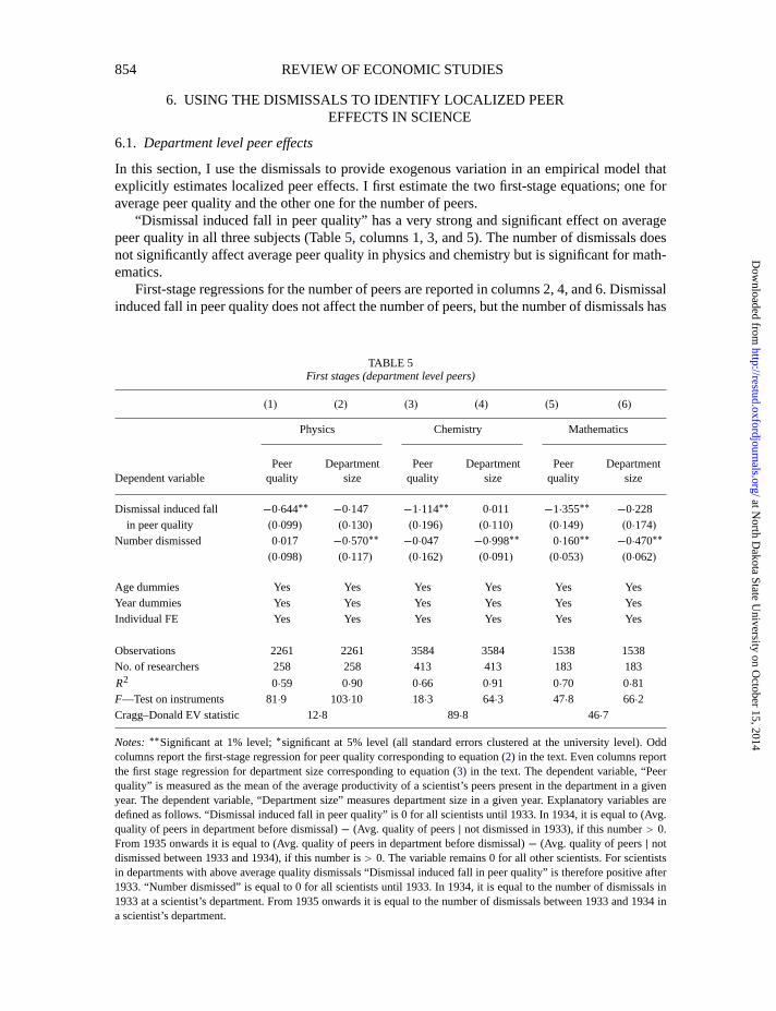
In this section, I use the dismissals to provide exogenous variation in an empirical model thatexplicitly estimates localized peer effects. I first estimate the two first-stage equations; one foraverage peer quality and the other one for the number of peers.

“Dismissal induced fall in peer quality” has a very strong and significant effect on averagepeer quality in all three subjects (Table5, columns 1, 3, and 5). The number of dismissals doesnot significantly affect average peer quality in physics and chemistry but is significant for math-ematics.

First-stage regressions for the number of peers are reported in columns 2, 4, and 6. Dismissalinduced fall in peer quality does not affect the number of peers, but the number of dismissals has

TABLE 5First stages (department level peers)

(1) (2) (3) (4) (5) (6)


Peer Department Peer Department Peer DepartmentDependent variable quality size quality size quality size

Dismissalinduced fall −0∙644∗∗ −0∙147 −1∙114∗∗ 0∙011 −1∙355∗∗ −0∙228in peer quality (0∙099) (0∙130) (0∙196) (0∙110) (0∙149) (0∙174)

Number dismissed 0∙017 −0∙570∗∗ −0∙047 −0∙998∗∗ 0∙160∗∗ −0∙470∗∗

(0∙098) (0∙117) (0∙162) (0∙091) (0∙053) (0∙062)


Observations 2261 2261 3584 3584 1538 1538No. of researchers 258 258 413 413 183 183

R2 0∙59 0∙90 0∙66 0∙91 0∙70 0∙81F—Test on instruments 81∙9 103∙10 18∙3 64∙3 47∙8 66∙2Cragg–Donald EV statistic 12∙8 89∙8 46∙7

Notes:∗∗Significantat 1% level;∗significantat 5% level (all standard errors clustered at the university level). Oddcolumns report the first-stage regression for peer quality corresponding to equation (2) in the text. Even columns reportthe first stage regression for department size corresponding to equation (3) in the text. The dependent variable, “Peerquality” is measured as the mean of the average productivity of a scientist’s peers present in the department in a givenyear. The dependent variable, “Department size” measures department size in a given year. Explanatory variables aredefined as follows. “Dismissal induced fall in peer quality” is 0 for all scientists until 1933. In 1934, it is equal to (Avg.quality of peers in department before dismissal)− (Avg. quality of peers| not dismissed in 1933), if this number> 0.From 1935 onwards it is equal to (Avg. quality of peers in department before dismissal)− (Avg. quality of peers| notdismissed between 1933 and 1934), if this number is> 0. The variable remains 0 for all other scientists. For scientistsin departments with above average quality dismissals “Dismissal induced fall in peer quality” is therefore positive after1933. “Number dismissed” is equal to 0 for all scientists until 1933. In 1934, it is equal to the number of dismissals in1933 at a scientist’s department. From 1935 onwards it is equal to the number of dismissals between 1933 and 1934 ina scientist’s department.

at North D



Dow

nloaded from


“rdr029” — 2012/4/17 — 12:44 — page 855 — #18


a strong and significant effect. This pattern is reassuring as it indicates that the dismissals indeedprovide two orthogonal instruments: one for average peer quality and one for department size.18

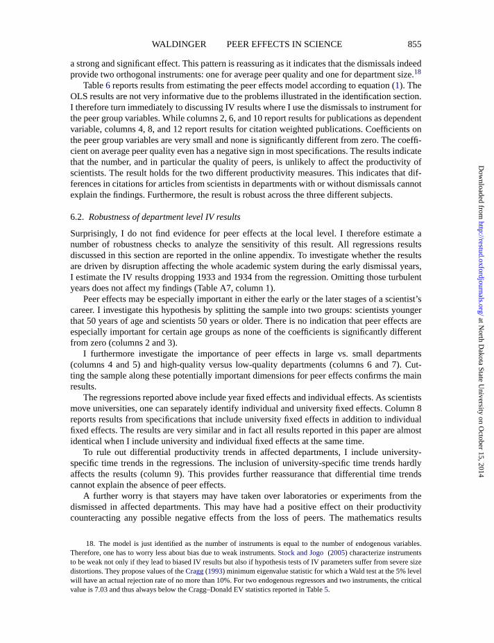
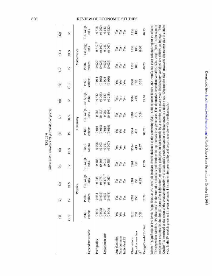
Table6 reports results from estimating the peer effects model according to equation (1). TheOLS results are not very informative due to the problems illustrated in the identification section.I therefore turn immediately to discussing IV results where I use the dismissals to instrument forthe peer group variables. While columns 2, 6, and 10 report results for publications as dependentvariable, columns 4, 8, and 12 report results for citation weighted publications. Coefficients onthe peer group variables are very small and none is significantly different from zero. The coeffi-cient on average peer quality even has a negative sign in most specifications. The results indicatethat the number, and in particular the quality of peers, is unlikely to affect the productivity ofscientists. The result holds for the two different productivity measures. This indicates that dif-ferences in citations for articles from scientists in departments with or without dismissals cannotexplain the findings. Furthermore, the result is robust across the three different subjects.

6.2. Robustness of department level IV results

Surprisingly, I do not find evidence for peer effects at the local level. I therefore estimate anumber of robustness checks to analyze the sensitivity of this result. All regressions resultsdiscussed in this section are reported in the online appendix. To investigate whether the resultsare driven by disruption affecting the whole academic system during the early dismissal years,I estimate the IV results dropping 1933 and 1934 from the regression. Omitting those turbulentyears does not affect my findings (Table A7, column 1).

Peer effects may be especially important in either the early or the later stages of a scientist’scareer. I investigate this hypothesis by splitting the sample into two groups: scientists youngerthat 50 years of age and scientists 50 years or older. There is no indication that peer effects areespecially important for certain age groups as none of the coefficients is significantly differentfrom zero (columns 2 and 3).

I furthermore investigate the importance of peer effects in large vs. small departments(columns 4 and 5) and high-quality versus low-quality departments (columns 6 and 7). Cut-ting the sample along these potentially important dimensions for peer effects confirms the mainresults.

The regressions reported above include year fixed effects and individual effects. As scientistsmove universities, one can separately identify individual and university fixed effects. Column 8reports results from specifications that include university fixed effects in addition to individualfixed effects. The results are very similar and in fact all results reported in this paper are almostidentical when I include university and individual fixed effects at the same time.

To rule out differential productivity trends in affected departments, I include university-specific time trends in the regressions. The inclusion of university-specific time trends hardlyaffects the results (column 9). This provides further reassurance that differential time trendscannot explain the absence of peer effects.

A further worry is that stayers may have taken over laboratories or experiments from thedismissed in affected departments. This may have had a positive effect on their productivitycounteracting any possible negative effects from the loss of peers. The mathematics results

18. The model is just identified as the number of instruments is equal to the number of endogenous variables.Therefore, one has to worry less about bias due to weak instruments.Stock and Jogo(2005) characterize instrumentsto be weak not only if they lead to biased IV results but also if hypothesis tests of IV parameters suffer from severe sizedistortions. They propose values of theCragg(1993) minimum eigenvalue statistic for which a Wald test at the 5% levelwill have an actual rejection rate of no more than 10%. For two endogenous regressors and two instruments, the criticalvalue is 7.03 and thus always below the Cragg–Donald EV statistics reported in Table5.

at North D



Dow

nloaded from


“rdr029” — 2012/4/17 — 12:44 — page 856 — #19


TAB

LE6

Inst

rum

en

talv

aria

ble

s(D

ep

art

me

ntl

eve

lpe

er

s)

(1)

(2)

(3)

(4)

(5)

(6)

(7)

(8)

(9)

(10)

(11)

(12)

OLS

IVO

LSIV

OLS

IVO

LSIV

OLS

IVO

LSIV

Phy

sics

Che

mis

try

Mat

hem

atic

s

Pub

li-P

ubli-

Cit.

wei

gt.

Cit.

wei

gt.

Pub

li-P

ubli-

Cit.

wei

gt.

Cit.

wei

gt.

Pub

li-P

ubli-

Cit.

wei

gt.

Cit.

wei

gt.

Dep

ende

ntva

riabl

e:ca

tions

catio

nsP

ubs.

Pub

s.ca

tions

catio

nsP

ubs.

Pub

s.ca

tions

catio

nsP

ubs.

Pub

s.

Pee

rqua

lity

0∙00

4−

0∙05

4−

0∙04

8−

0∙48

80∙

006

−0∙

010

0∙08

5−

0∙34

20∙

014

−0∙

022

0∙51

7∗∗

0∙31

8(0

∙005

)(0

∙035

)(0

∙075

)(0

∙496

)(0

∙003

(0∙0

15)

(0∙0

57)

(0∙2

65)

(0∙0

15)

(0∙0

26)

(0∙1

67)

(0∙2

62)

Dep

artm

ents

ize

−0∙

007

0∙03

5−

0∙17

7∗∗

0∙01

6−

0∙01

10∙

019

0∙08

90∙

147

0∙00

40∙

032

0∙04

10∙

143

(0∙0

04)

(0∙0

34)

(0∙0

62)

(0∙5

53)

(0∙0

07)

(0∙0

10)

(0∙1

93)

(0∙2

18)

(0∙0

10)

(0∙0

26)

(0∙0

67)

(0∙3

22)

Age

dum

mie

sY

esY

esY

esY

esY

esY

esY

esY

esY

esY

esY

esY

esY

ear

dum

mie

sY

esY

esY

esY

esY

esY

esY

esY

esY

esY

esY

esY

esIn

divi

dual

FE

Yes

Yes

Yes

Yes

Yes

Yes

Yes

Yes

Yes

Yes

Yes

Yes

Obs

erva

tions

2261

2261

2261

2261

3584

3584

3584

3584

1538

1538

1538

1538

No.

ofre

sear

cher

s25

825

825

825

841

341

341

341

318

318

318

318

3R

20∙

390∙

250∙

670∙

540∙

320∙

20C

ragg

–Don

ald

EV

Sta

t.12

.79

12.7

989

.76

89.7

646

.73

46.7

3

No

tes:

∗∗S

igni

fican

tat

1%le

vel;∗

sign

ifica

ntat

5%le

vel(

alls

tand

ard

erro

rscl

uste

red

atth

eun

iver

sity

leve

l).O

ddco

lum

nsre

port

OLS

resu

ltsan

dev

enco

lum

nsre

port

IVre

sults

.T

hede

pend

ent

varia

ble,

“Pub

licat

ions

”is

the

sum

ofa

scie

ntis

t’spu

blic

atio

nsin

top

jour

nals

ina

give

nye

ar.

The

alte

rnat

ive

depe

nden

tva

riabl

e,“C

it.w

eigt

.P

ubs.

”is

the

sum

ofsu

bseq

uent

cita

tions

(inth

efir

st50

year

saf

ter

publ

icat

ion)

toar

ticle

spu

blis

hed

into

pjo

urna

lsby

asc

ient

ist

ina

give

nye

ar.

Exp

lana

tory

varia

bles

are

defin

edas

follo

ws.

“Pee

rQ

ualit

y”is

mea

sure

das

the

mea

nof

the

aver

age

prod

uctiv

ityof

asc

ient

ist’s

peer

spr

esen

tin

the

depa

rtm

enti

na

give

nye

ar.“

Dep

artm

ents

ize”

mea

sure

sde

part

men

tsiz

ein

agi

ven

year

.In

the

IVm

odel

spr

esen

ted

inev

enco

lum

ns,I

inst

rum

entf

orpe

erqu

ality

and

depa

rtm

ents

ize

with

the

dism

issa

ls.

at North D



Dow

nloaded from


“rdr029” — 2012/4/17 — 12:44 — page 857 — #20


should not be contaminated by such behaviour and are indeed very similar to the results forthe other two subjects. An additional way of exploring whether taking over laboratories may bedriving the results is to estimate the regression for theoretical physicists only. Even though theresults are less precisely estimated, the findings show no evidence for peer effects in theoreticalphysics (column 10).

Using the dismissals as instrumental variables relies on the assumption that the dismissalsonly affected scientists’ productivity through its effect on the researchers’ peer groups. It is im-portant to note that any factor affecting all researchers in Germany in a similar way, such asa possible decline of journal quality, will be captured by the year fixed effects and would thusnot invalidate the identification strategy. Because unaffected departments act as a control group,only factors changing at the same time as the dismissal and exclusively affecting departmentswith dismissals (or only those without dismissals) may be potential threats to the identificationstrategy. Most of the potentially worrying biases, such as disruption effects or increased teachingloads, would bias the IV estimates in favour of finding peer effects. As I do not find evidencefor localized peer effects, one has to worry less about these biases. Some violations of the ex-clusion restriction, however, would lead me to underestimate peer effects. In results discussed inmore detail in the online appendix (Appendix 1 and Table A8), I show that the dismissals wereunrelated to changes in promotion incentives. Furthermore, the dismissals were not related tothe probability that stayers left the sample for retirement or other reasons. I also show that thenumber of ardent Nazi supporters, who could have benefited from preferential treatment by theNazi government, was not related to the dismissals. Finally, I show that changes in fundingare unlikely to drive my results.

6.3. Specialization level peer effects

The definition of the peer group in the previous regressions was based on all peers in a scientist’sdepartment. It is, however, possible that the productivity of scientists is only affected by peerswho work in very similar fields. To investigate this hypothesis, I use the scientists specializationto define their peer group. According to this definition of the peer group, the relevant peers ofan experimental physicist are only the other experimentalists in his department, not theoreticalphysicists, technical physicists, or astrophysicists.

Similar to the department level results, the coefficients on the peer group variables are verysmall and none of them is significantly different from zero (Table7).19 Furthermore,the coeffi-cients on peer quality mostly have the wrong sign if one were expecting positive peer effects. Theresults for mathematics are less precisely estimated because most mathematicians did not confinetheir research to only one or two specializations. Many of them were working on very differenttopics that even today cannot be precisely assigned to particular specializations. Nonetheless,there is no evidence for any significant peer effects in mathematics. It may be possible that lo-calized peer effects occur in even more specialized subfields. As the mean number of researchersin the specializations I consider here is about 3.5, these even smaller subfields would have to beextremely specialized.

6.4. Peer effects from high-quality peers

Recent research on life scientists in the U.S. has indicated that star scientists have a particularlylarge impact on co-authors (Azoulayet al.,2010). In the previous regressions, I have investigatedhow average peer quality affects productivity. It may well be the case that only colleagues of veryhigh quality affect the productivity of scientists.

19. First-stage regressions for the specialization level results are reported in Table A9 in the online appendix.

at North D



Dow

nloaded from


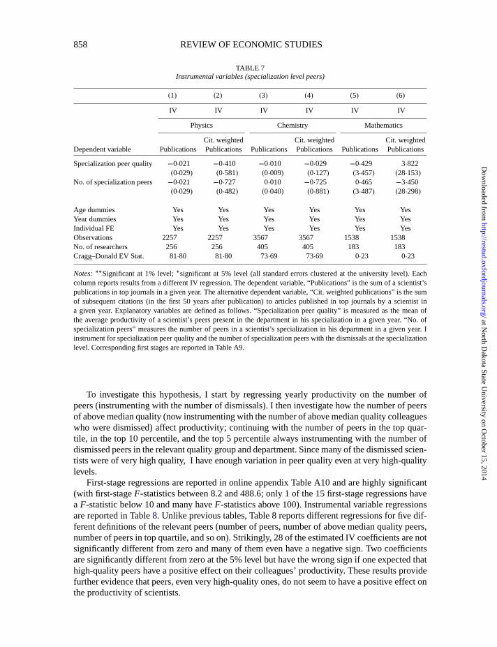
“rdr029” — 2012/4/17 — 12:44 — page 858 — #21


TABLE 7Instrumental variables (specialization level peers)

(1) (2) (3) (4) (5) (6)

IV IV IV IV IV IV


Cit. weighted Cit. weighted Cit. weightedDependent variable Publications Publications Publications Publications PublicationsPublications

Specializationpeer quality −0∙021 −0∙410 −0∙010 −0∙029 −0∙429 3∙822(0∙029) (0∙581) (0∙009) (0∙127) (3∙457) (28∙153)

No. of specialization peers −0∙021 −0∙727 0∙010 −0∙725 0∙465 −3∙450(0∙029) (0∙482) (0∙040) (0∙881) (3∙487) (28∙298)

Age dummies Yes Yes Yes Yes Yes YesYear dummies Yes Yes Yes Yes Yes YesIndividual FE Yes Yes Yes Yes Yes YesObservations 2257 2257 3567 3567 1538 1538No. of researchers 256 256 405 405 183 183Cragg–Donald EV Stat. 81∙80 81∙80 73∙69 73∙69 0∙23 0∙23

Notes:∗∗Significantat 1% level;∗significantat 5% level (all standard errors clustered at the university level). Eachcolumn reports results from a different IV regression. The dependent variable, “Publications” is the sum of a scientist’spublications in top journals in a given year. The alternative dependent variable, “Cit. weighted publications” is the sumof subsequent citations (in the first 50 years after publication) to articles published in top journals by a scientist ina given year. Explanatory variables are defined as follows. “Specialization peer quality” is measured as the mean ofthe average productivity of a scientist’s peers present in the department in his specialization in a given year. “No. ofspecialization peers” measures the number of peers in a scientist’s specialization in his department in a given year. Iinstrument for specialization peer quality and the number of specialization peers with the dismissals at the specializationlevel. Corresponding first stages are reported in Table A9.

To investigate this hypothesis, I start by regressing yearly productivity on the number ofpeers (instrumenting with the number of dismissals). I then investigate how the number of peersof above median quality (now instrumenting with the number of above median quality colleagueswho were dismissed) affect productivity; continuing with the number of peers in the top quar-tile, in the top 10 percentile, and the top 5 percentile always instrumenting with the number ofdismissed peers in the relevant quality group and department. Since many of the dismissed scien-tists were of very high quality, I have enough variation in peer quality even at very high-qualitylevels.

First-stage regressions are reported in online appendix Table A10 and are highly significant(with first-stageF-statistics between 8.2 and 488.6; only 1 of the 15 first-stage regressions havea F-statistic below 10 and many haveF-statistics above 100). Instrumental variable regressionsare reported in Table8. Unlike previous tables, Table 8 reports different regressions for five dif-ferent definitions of the relevant peers (number of peers, number of above median quality peers,number of peers in top quartile, and so on). Strikingly, 28 of the estimated IV coefficients are notsignificantly different from zero and many of them even have a negative sign. Two coefficientsare significantly different from zero at the 5% level but have the wrong sign if one expected thathigh-quality peers have a positive effect on their colleagues’ productivity. These results providefurther evidence that peers, even very high-quality ones, do not seem to have a positive effect onthe productivity of scientists.

at North D



Dow

nloaded from


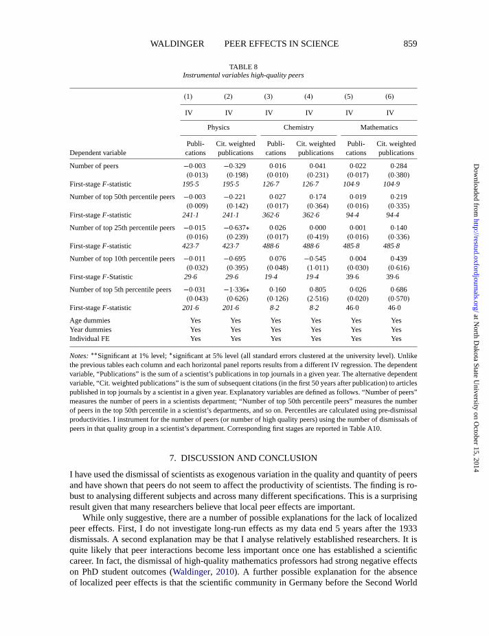
“rdr029” — 2012/4/17 — 12:44 — page 859 — #22


TABLE 8Instrumental variables high-quality peers

(1) (2) (3) (4) (5) (6)

IV IV IV IV IV IV


Publi- Cit. weighted Publi- Cit. weighted Publi- Cit. weightedDependent variable cations publications cations publications cationspublications

Numberof peers −0∙003 −0∙329 0∙016 0∙041 0∙022 0∙284(0∙013) (0∙198) (0∙010) (0∙231) (0∙017) (0∙380)

First-stageF-statistic 195∙5 195∙5 126∙7 126∙7 104∙9 104∙9

Number of top 50th percentile peers−0∙003 −0∙221 0∙027 0∙174 0∙019 0∙219(0∙009) (0∙142) (0∙017) (0∙364) (0∙016) (0∙335)


Number of top 25th percentile peers−0∙015 −0∙637∗ 0∙026 0∙000 0∙001 0∙140(0∙016) (0∙239) (0∙017) (0∙419) (0∙016) (0∙336)


Number of top 10th percentile peers−0∙011 −0∙695 0∙076 −0∙545 0∙004 0∙439(0∙032) (0∙395) (0∙048) (1∙011) (0∙030) (0∙616)

First-stageF-Statistic 29∙6 29∙6 19∙4 19∙4 39∙6 39∙6

Number of top 5th percentile peers −0∙031 −1∙336∗ 0∙160 0∙805 0∙026 0∙686(0∙043) (0∙626) (0∙126) (2∙516) (0∙020) (0∙570)



Notes:∗∗Significantat 1% level;∗significantat 5% level (all standard errors clustered at the university level). Unlikethe previous tables each column and each horizontal panel reports results from a different IV regression. The dependentvariable, “Publications” is the sum of a scientist’s publications in top journals in a given year. The alternative dependentvariable, “Cit. weighted publications” is the sum of subsequent citations (in the first 50 years after publication) to articlespublished in top journals by a scientist in a given year. Explanatory variables are defined as follows. “Number of peers”measures the number of peers in a scientists department; “Number of top 50th percentile peers” measures the numberof peers in the top 50th percentile in a scientist’s departments, and so on. Percentiles are calculated using pre-dismissalproductivities. I instrument for the number of peers (or number of high quality peers) using the number of dismissals ofpeers in that quality group in a scientist’s department. Corresponding first stages are reported in Table A10.

7. DISCUSSION AND CONCLUSION

I have used the dismissal of scientists as exogenous variation in the quality and quantity of peersand have shown that peers do not seem to affect the productivity of scientists. The finding is ro-bust to analysing different subjects and across many different specifications. This is a surprisingresult given that many researchers believe that local peer effects are important.

While only suggestive, there are a number of possible explanations for the lack of localizedpeer effects. First, I do not investigate long-run effects as my data end 5 years after the 1933dismissals. A second explanation may be that I analyse relatively established researchers. It isquite likely that peer interactions become less important once one has established a scientificcareer. In fact, the dismissal of high-quality mathematics professors had strong negative effectson PhD student outcomes (Waldinger, 2010). A further possible explanation for the absenceof localized peer effects is that the scientific community in Germany before the Second World

at North D



Dow

nloaded from


“rdr029” — 2012/4/17 — 12:44 — page 860 — #23


War was very integrated. Conferences were common and scientists were very mobile withinGermany. Geographic location of researchers may therefore not have been very important formore established researchers. A further reason for the absence of localized peer effects may bethat science is much more specialized than other subjects such as economics.

An important question is whether evidence on peer effects in the 1920s and 1930s can helpus understand peer interactions today. A number of reasons suggest that the findings of thisstudy may be relevant for understanding spillovers among present-day researchers. The threesubjects studied in this paper were already well established at that time, especially in Germany.In fact, Germany was the leading country for scientific research in the first decades of the 20thcentury. If peer effects are an important determinant of scientific productivity, they are likelyto be especially important in a flourishing research environment such as Germany in the early20th century. Scientific research at the time followed practices and conventions that were verysimilar to current research methods. Scientists were publishing their results in refereed aca-demic journals, conferences were common, and researchers were surprisingly mobile within theGerman-speaking scientific community. Unlike today, they could not communicate via E-mail.They did, however, vividly discuss their research in very frequent mail correspondence with theircolleagues in other universities.

Recent research on today’s scientists also seems to suggest that localized spillovers are un-likely to be important.Dubois et al. (2010) show that localized spillovers do not affect theproductivity of mathematicians between 1984 and 2006. Furthermore,Azoulay et al. (2010)find that the loss of a local co-author does not have a larger impact on the productivity of lifescientists than losing a co-author who was located in a different university.

The question remains why scientists behave as if local peers are a key input in the ideas pro-duction process. One potential explanation is that being surrounded by esteemed peers is purelya private benefit,i.e. it enters a scientist’s utility function but does not affect his productivity.Another explanation could be that localized spillovers are important but they are extremely lo-calized.

Acknowledgement.Christoph König and Michael Talbot provided excellent research assistance. I thank the editorImran Rasul and three anonymous referees for very helpful comments. I also thank Pierre Azoulay, Oriana Bandiera,Marianne Bertrand, Luis Garicano, Michael Greenstone, Jennifer Hunt, Victor Lavy, Guy Michaels, Ted Miguel, AndrewOswald, Matthias Parey, Barbara Petrongolo, Justin Smith, Daniel Sturm and especially David Card and Steve Pischkefor very helpful comments and suggestions. John Andraos, Cathrin Carson, Ute Deichmann, Klaus Fischer, ReinhardSiegmund-Schulze, Richard Staley, and David Wilkins provided very valuable information on historical details. I amgrateful for comments received from seminar participants in Bergen, Berkeley, Bocconi, Bonn, Cambridge, Essex,Helsinki, INSEAD, LSE, Munich, QMUL, Toronto, Uppsala, Utrecht, Warwick, UCL, the NBER SI, the RES con-ference (Warwick), the CEP conference (Cambridge), the ZEW conference (Mannheim), the "Knowledge for Growth"conference (Toulouse), the BRICK-DIME Workshop (Carlo Alberto), the EEA Conference (Milan), the IZA/CEPRESSLE (Ammersee), the Verein für Socialpolitik (Kiel), the SOLE conference (London), and the CESifo conference(Munich).

SupplementaryData

Supplementary data are available atReview of Economic Studiesonline.

REFERENCES

AMERICAN ASSOCIATION OF THE ADVANCEMENT OF SCIENCE (1941), “Physics in Pre-Nazi Germany”,Sci-ence,94, 488–489.

ADAMS, J. D., BLACK, G. C., CLEMMONS J. R. and STEPHAN, P. E. (2005), “Scientific Teams and InstitutionalCollaborations: Evidence from U.S. Universities, 1981–1999”,Research Policy, 34, 259–285.

AGRAWAL, A. and AVI, G. (2008), “Restructuring Research: Communication Costs and the Democratization of Uni-versity Innovation”,The American Economic Review, 98, 1578–1590.

at North D



Dow

nloaded from


“rdr029” — 2012/4/17 — 12:44 — page 861 — #24


AZOULAY, P., ZIVIN, J. G. and WANG, J. (2010), “Superstar Extinction”,The Quarterly Journal of Economics, 125,549–589.

BANDIERA, O., BARANKAY, I., RASUL, I. (2010), “Social Incentives in the Workplace”,The Review of EconomicStudies,77, 417–458.

BEYERCHEN, A. D. (1977),Scientists Under Hitler—Politics and the Physics Community in the Third Reich(NewHaven: Yale University Press).

BIOGRAPHISCHES HANDBUCH DER DEUTSCHPRACHIGEN EMIGRATION NACH 1933–1945/INTERNA-TIONAL BIOGRAPHICAL DICTIONARZ OF CENTRAL EUROPEAN EMIGRES 1933–1945 (1983), in Her-bert A. Strauss and Werner Röder (eds)Vol. 2 The Arts Sciences and Literature, Institut fur Zeitgeschichte, Munchen,Research Foundation for Jewish Immigration, New York(Müchen: KG Saur verlag).

CRAGG, J. G. and DONALD, S. G. (1993), “Testing Identifiablility and Specification in Instrumental Variables Mod-els”, Econometric Theory,9, 222–240.

DEICHMANN, U. (2001),Flüchten, Mitmachen, Vergessen—Chemiker und Biochemiker in der NS-Zeit(Weinheim,Germany: Wiley-VCH Verlag).

DUBOIS, P., ROCHET, J.-C. and Schlenker, J-M. (2010), “Productivity and Mobility in Academic Research: Evidencefrom Mathematicians” (Mimeo, Toulouse School of Economics).

FISCHER, K. (1991), “Die Emigration deutschsprachiger Physiker nach 1933: Stukturen und Wirkungen”, in Strauss,H. A., Fischer, K., Hoffmann, C. and Söllner, A. (eds)Die Emigration der Wissenschaften nach 1933(München: K.G. Saur Verlag ) 27–72.

HARTSHORNE, E. Y. (1937),The German Universities and National Socialism(Cambridge: Harvard University Press).HENTSCHEL, K. (1996),Physics and National Socialism—An Anthology of Primary Sources(Berlin: Birkhäuser

Verlag).IMBENS, G. and ANGRIST, J. (1994), “Identification and Estimation of Local Average Treatment Effects”,Economet-

rica, 62, 467–475.KIM, E. H., MORSE, A. and ZINGALES, L. (2009), “Are Elite Universities Losing their Competitive Edge”,Journal

of Financial Economics,93, 353–381.KRÖNER, P. (1983),Vor fünfzig Jahren—Die Emigration deutschsprachiger Wissenschaftler 1933–1939,in Gesell-

schaft für Wissenschaftsgeschichte Münster (Wolfenbüttel: Heckners Verlag).MAS, A. and MORETTI, E. (2009), “Peers at Work”,The American Economic Review, 99, 112–145.NOTGEMEINSCHAFT DEUTSCHER WISSENSCHAFTLER AUSLAND (ed) (1937),List of Displaced German

Scholars(London).OETTL, A. (2009), “Productivity and Helpfulness: Implications of a New Taxonomy for Star Scientists” (Mimeo, Geor-

gia Tech).ROSENBLAT, T. S. and MOBIUS, M. M. (2004), “Getting Closer or Drifting Apart?”Quarterly Journal of Economics,

119, 971–1009.SANTOS SILVA, J. M. C. and TENREYRO, S. (2010), “On the Existence of the Maximum Likelihood Estimates in

Poisson Regression”,Economics Letters, 107, 310–312.SANTOS SILVA, J. M. C. and TENREYRO, S. (2011), “Poisson: Some Convergence Issues”,STATA Journal,

11, 215–225.SIEGMUND-SCHULTZE, R. (1998),Mathematiker auf der Flucht vor Hitler,Deutsche Mathematiker Vereinigung, F.

Vieweg.SIMONSOHN, G. (2007), “Die Deutsche Physikalische Gesellschaft und die Forschung”, in Hoffmann, D. and Walker,

M. (eds)Physiker zwischen Autonomie und Anpassung—Die Deutsche Physikalische Gesellschaft im Dritten Reich(Weinheim: Wiley-VHC Verlag).

STOCK, J. H. and JOGO, M. (2005), “Testing for Weak Instruments in Linear IV Regression, in Andrews, D. W. K.and Stock, J. H. (eds)Identification and Inference for Econometric Models: Essays in Honor of Thomas Rothenberg(New York: Cambridge University Press).

WALDINGER, F. (2010), “Quality Matters—The Expulsion of Professors and the Consequences for Ph.D. StudentOutcomes in Nazi Germany”,Journal of Political Economy, 118, 787–831.

WEINBERG, B. A. (2007), “Geography and Innovation: Evidence from Nobel Laureate Physicists” (Mimeo, OhioState University).

at North D



Dow

nloaded from


Documents

Peer Effects in Science: Evidence from the Dismissal of Scientists in Nazi Germany