PERFECT COMPETITION - virtualpanic.comvirtualpanic.com/anonymousftplistings/ebooks/ECONOMICS/8 - Perfect...ers and sellers come together, ... may think of an intense, personal rivalry,

No one knows exactly how many different types of goods and services are of-fered for sale in the United States, but the number must be somewhere inthe tens of millions. Each of these goods is traded in a market, where buy-

ers and sellers come together, and these markets have several things in common.Sellers want to sell at the highest possible price; buyers seek the lowest possibleprice; and all trade is voluntary. But here, the similarity ends.

When we observe buyers and sellers in action, we see that different goods andservices are sold in vastly different ways. Take advertising, for example. Every day,we are inundated with sales pitches on television, radio, and newspapers for a longlist of products: toothpaste, perfume, automobiles, Internet Web sites, cat food,banking services, and more. But have you ever seen a farmer on television, tryingto convince you to buy his wheat, rather than the wheat of other farmers? Doshareholders of major corporations like General Motors sell their stock by adver-tising in the newspaper? Why, in a world in which virtually everything seems to beadvertised, do we not see ads for wheat, corn, crude oil, gold, copper, shares ofstock, or foreign currency?

Or consider profits. Anyone starting a business hopes to make as much profitas possible. Yet some companies—Microsoft, Quaker Oats, and Pepsico, for ex-ample—earn sizable profit for their owners year after year, while at other compa-nies, such as Trans World Airlines and most small businesses, economic profit isgenerally low.

We could say, “That’s just how the cookie crumbles,” and attribute all of theseobservations to pure randomness. But economics is all about explaining suchthings—finding patterns amidst the chaos of everyday economic life. When econo-mists turn their attention to differences in trading, such as these, they think imme-diately about market structure:

To determine the structure of any particular market, we begin by asking threesimple questions:

PERFECT COMPETITION

CHAPTER

8CHAPTER OUTLINE

What Is Perfect Competition?The Three Requirements for

Perfect CompetitionIs Perfect Competition Realistic?

The Perfectly Competitive FirmGoals and Constraints of the

Competitive FirmCost and Revenue Data for a

Competitive FirmFinding the Profit-Maximizing

Output LevelMeasuring Total ProfitThe Firm’s Short-Run Supply

Curve

Competitive Markets in theShort Run

The (Short-Run) Market SupplyCurve

Short-Run Equilibrium

Competitive Markets in theLong Run

Profit and Loss and the Long RunLong-Run EquilibriumThe Notion of Zero Profit in

Perfect CompetitionPerfect Competition and Plant

SizeA Summary of the Competitive

Firm in the Long Run

What Happens When ThingsChange?

A Change in DemandMarket Signals and the Economy

Using the Theory: Changes inTechnology

By market structure, we mean all the characteristics of a market that influ-ence the behavior of buyers and sellers when they come together to trade.

Market structure The character-istics of a market that influencehow trading takes place.

What Is Perfect Competition? 215

1. How many buyers and sellers are there in the market?2. Is each seller offering a standardized product, more or less indistinguishable

from that offered by other sellers, or are there significant differences betweenthe products of different firms?

3. Are there any barriers to entry or exit, or can outsiders easily enter and leavethis market?

The answers to these questions help us to classify a market into one of four basictypes: perfect competition, monopoly, monopolistic competition, or oligopoly. Thesubject of this chapter is perfect competition. In the next two chapters, we’ll lookcarefully at the other market structures.

WHAT IS PERFECT COMPETITION?

Does the phrase “perfect competition” sound familiar? It should, because you en-countered it earlier, in Chapter 3. There you learned (briefly) that the famoussupply and demand model explains how prices are determined in perfectly com-petitive markets. Now we’re going to take a much deeper and more comprehen-sive look at perfectly competitive markets. By the end of this chapter, you willunderstand very clearly how perfect competition and the supply and demandmodel are related.

Let’s start with the word “competition” itself. When you hear that word, youmay think of an intense, personal rivalry, like that between two boxers competingin a ring or two students competing for the best grade in a small class. But there areother, less personal forms of competition. If you took the SAT exam to get into col-lege, you were competing with thousands of other test takers in rooms just likeyours, all across the country. But the competition was impersonal: You were tryingto do the best that you could do, trying to outperform others in general, but notcompeting with any one individual in the room. In economics, the term “competi-tion” is used in the latter sense. It describes a situation of diffuse, impersonal com-petition in a highly populated environment. The market structure you will learnabout in this chapter—perfect competition—is an example of this notion.

THE THREE REQUIREMENTS OF PERFECT COMPETITION

These three conditions probably raise more questions than they answer, so let’s seewhat each one really means.

A Large Number of Buyers and Sellers. In perfect competition, there must bemany buyers and sellers. How many? It would be nice if we could specify a num-ber—like 32,456—for this requirement. Unfortunately, we cannot, since what con-stitutes a large number of buyers and sellers can be different under different condi-tions. What is important is this:

Perfect competition is a market structure with three important characteristics:

1. There are large numbers of buyers and sellers, and each buys or sells only a tiny fraction of the total quantity in the market.

2. Sellers offer a standardized product.3. Sellers can easily enter into or exit from the market.

Perfect competition A marketstructure in which there are manybuyers and sellers, the product is standardized, and sellers caneasily enter or exit the market.

Characterize the Market

Think of the world market for wheat. On the selling side, there are hundreds ofthousands of individual wheat farmers—more than 250,000 in the United Statesalone. Each of these farmers produces only a tiny fraction of the total market quan-tity. If any one of them were to double, triple, or even quadruple its production, theimpact on total market quantity and market price would be negligible. The same istrue on the buying side: There are so many small buyers that no one of them can af-fect the market price by increasing or decreasing its quantity demanded.

Most agricultural markets conform to the large-number/small-participant re-quirement, as do markets for precious metals such as gold and silver and marketsfor the stocks and bonds of large corporations. For example, more than 2 millionshares of General Motors stock are bought and sold every day, at a price (as this iswritten) of about $70 per share. A decision by a single stockholder to sell say, $1 million dollars worth of this stock—about 14,000 shares—would cause only abarely noticeable change in quantity supplied on any given day.

But now think about the U.S. market for athletic shoes. Here, four large pro-ducers—Nike, Reebok, Adidas, and FILA—account for 75 percent of total sales. Ifany one of these producers decided to change its output by even 10 percent, the im-pact on total quantity supplied—and market price—would be very noticeable. Themarket for athletic shoes thus fails the large-number/small-participant requirement,so it is not an example of perfect competition.

A Standardized Product Offered by Sellers. In a perfectly competitive mar-ket, buyers do not perceive significant differences between the products of oneseller and another. For example, buyers of wheat will ordinarily have no prefer-ence for one farmer’s wheat over another’s, so wheat would surely pass the stan-dardized product test. The same is true of many other agricultural products—corn syrup and soybeans. It is also true of commodities like crude oil or porkbellies, precious metals like gold or silver, and financial instruments such as thestocks and bonds of a particular firm. (One share of AT&T stock is indistinguish-able from another.)

When buyers do notice significant differences in the outputs of different sellers,the market is not perfectly competitive. For example, most consumers perceive dif-ferences among the various brands of coffee on the supermarket shelf and may havestrong preferences for one particular brand. Coffee, therefore, fails the standardizedproduct test of perfect competition. Other goods and services that would fail thistest include personal computers, automobiles, houses, colleges, and medical care.

Easy Entry into and Exit from the Market. Entry into a market is rarely free—anew seller must always incur some costs to set up shop, begin production, and es-tablish contacts with customers. But a perfectly competitive market has no signifi-cant barriers to discourage new entrants: Any firm wishing to enter can do businesson the same terms as firms that are already there. For example, anyone with theright background in farming can begin planting and growing wheat by paying thesame costs as veteran wheat farmers. The same is true of anyone wishing to openup a dry cleaning shop, a new restaurant, or an E-commerce consulting firm forcompanies that want to sell more effectively over the Internet. Each of these exam-ples would pass the free-entry test of perfect competition.

216 Chapter 8 Perfect Competition

In a perfectly competitive market, the number of buyers and sellers is so largethat no individual decision maker can significantly affect the price of the prod-uct by changing the quantity it buys or sells.

What Is Perfect Competition? 217

In many markets, however, there are significant barriers to entry. These are oftenimposed by government. Sometimes, the government imposes absolute restrictionson the number of market participants allowed. For example, the number of taxicabslicensed to operate in New York City is fixed, determined by the city government.From the 1930s until 1996, this number was set at 11,787. In the late 1990s, the cityfinally increased the number of taxi licenses, but only by a few hundred, bringing thetotal to 12,187. Unless the city issues more licenses in the future, true entry into thismarket will be impossible—the licenses may change hands, but the total number oflegally operated taxis cannot increase. Another example of government barriers toentry is zoning laws. These place strict limits on how many businesses such as movietheaters, supermarkets, or hotels can operate in a local area.

Barriers to entry can also arise without any government action, simply becauseexisting sellers have an important advantage new entrants cannot duplicate. Thebrand loyalty enjoyed by existing producers of breakfast cereals, instant coffee, andsoft drinks would require a new entrant to wrest customers away from existingfirms—a very costly undertaking. Or significant economies of scale may give exist-ing firms a cost advantage over new entrants. We will discuss these and other barri-ers to entry in more detail in later chapters.

In addition to easy entry, perfect competition requires easy exit: A firm sufferinga long-run loss must be able to sell off its plant and equipment and leave the indus-try for good, without obstacles. Some markets satisfy this requirement, and somedo not. Plant-closing laws or union agreements can require lengthy advance noticeand high severance pay when workers are laid off. Or capital equipment may be sohighly specialized—like an assembly line designed to produce just one type of auto-mobile—that it cannot be sold off if the firm decides to exit the market. These andother barriers to exit do not conform to the assumptions of perfect competition.

IS PERFECT COMPETITION REALISTIC?The three assumptions a market must satisfy to be perfectly competitive (or just“competitive,” for short) are rather restrictive. Do any markets satisfy all these re-quirements? How broadly can we apply the model of perfect competition when wethink about the real world?

First, remember that perfect competition is a model—an abstract representationof reality. No model can capture all of the details of a real-world market, nor shouldit. Still, in some cases, the model fits remarkably well. We have seen that the marketfor wheat, for example, passes all three tests for a competitive market: many buyersand sellers, standardized output, and easy entry and exit. Indeed, most agriculturalmarkets satisfy the strict requirements of perfect competition quite closely, as domany financial markets and some markets for consumer goods and services.

But in the vast majority of markets, one or more of the assumptions of perfectcompetition will, in a strict sense, be violated. This might suggest that the modelcan be applied only in a few limited cases. Yet when economists look at real-worldmarkets, they use perfect competition more often than any other market structure.Why is this?

First, with perfect competition, we can use simple techniques to make somestrong predictions about a market’s response to changes in consumer tastes, tech-nology, and government policies. While other types of market structure models alsoyield valuable predictions, they are often more cumbersome and their predictionsless definitive. Second, economists believe that many markets—while not strictlyperfectly competitive—come reasonably close. The more closely a real-world mar-ket fits the model, the more accurate our predictions will be when we use it.

We can even—with some caution—use the model to analyze markets that vio-late all three assumptions. Take the worldwide market for television sets. There areabout a dozen major sellers in this market. Each of them knows that its output de-cisions will have some effect on the market price, but no one of them can have amajor impact on price. Consumers do recognize the difference between one brandand another, but their preferences are not very strong, and most recognize that qual-ity has become so standardized that all brands are actually close substitutes for eachother. And there are indeed barriers to entry—existing firms have supply and distri-bution networks that would be difficult for new entrants to replicate—but thesebarriers are not so great that they would keep out new entrants in the face of highpotential profit. Thus, although the market for televisions does not strictly satisfyany of the requirements of perfect competition, it is not too far off on any one ofthem. The model will not perform as accurately for televisions as it does for wheat,but, depending on how much accuracy we need, it may do just fine.

In sum, perfect competition can approximate conditions and yield accurate-enough predictions in a wide variety of markets. This is why you will often findeconomists using the model to analyze the markets for crude oil, consumer elec-tronic goods, fast-food meals, medical care, and higher education, even though ineach of these cases one or more of the requirements may not be strictly satisfied.

THE PERFECTLY COMPETITIVE FIRM

When we stand at a distance and look at conditions in a competitive market, weget one view of what is occurring; when we stand close and look at the individualcompetitive firm, we get an entirely different picture. But these two pictures arevery closely related. After all, a market is a collection of individual decision mak-ers, much as a human body is a collection of individual cells. In a perfectly compet-itive market, the individual cells of firms and consumers and the overall body of themarket affect each other through a variety of feedback mechanisms. This is why, inlearning about the competitive firm, we must also discuss the competitive marketin which it operates.

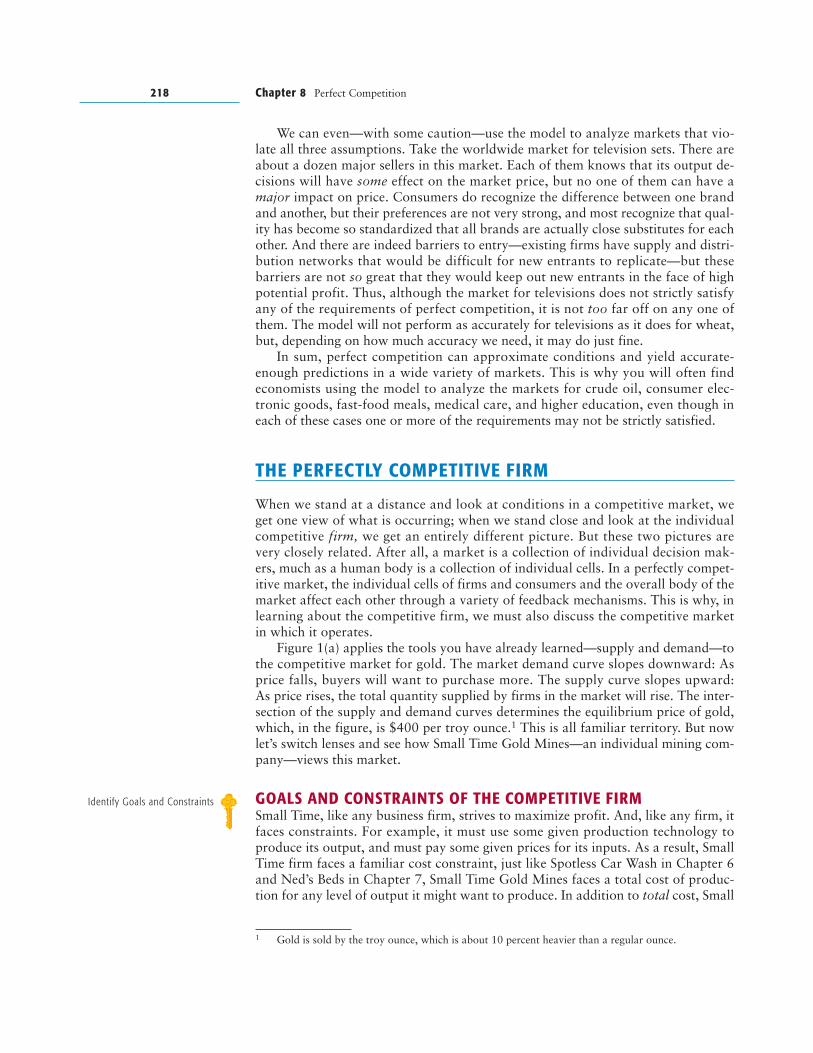
Figure 1(a) applies the tools you have already learned—supply and demand—tothe competitive market for gold. The market demand curve slopes downward: Asprice falls, buyers will want to purchase more. The supply curve slopes upward: As price rises, the total quantity supplied by firms in the market will rise. The inter-section of the supply and demand curves determines the equilibrium price of gold,which, in the figure, is $400 per troy ounce.1 This is all familiar territory. But nowlet’s switch lenses and see how Small Time Gold Mines—an individual mining com-pany—views this market.

GOALS AND CONSTRAINTS OF THE COMPETITIVE FIRMSmall Time, like any business firm, strives to maximize profit. And, like any firm, itfaces constraints. For example, it must use some given production technology toproduce its output, and must pay some given prices for its inputs. As a result, SmallTime firm faces a familiar cost constraint, just like Spotless Car Wash in Chapter 6and Ned’s Beds in Chapter 7, Small Time Gold Mines faces a total cost of produc-tion for any level of output it might want to produce. In addition to total cost, Small


1 Gold is sold by the troy ounce, which is about 10 percent heavier than a regular ounce.

Identify Goals and Constraints

The Perfectly Competitive Firm 219

Time has ATC, AVC, and MC curves, and these have the familiar shapes youlearned about in the previous two chapters.

In addition to a cost constraint, Small Time Gold Mines faces a demand con-straint, as does any firm. But there is something different about the demand con-straint for a perfectly competitive firm like Small Time.

The Demand Curve Facing a Perfectly Competitive Firm. Panel (b) of Figure 1shows the demand curve facing Small Time Gold Mines. Notice the special shape ofthis curve: It is horizontal, or infinitely price elastic. This tells us that no matter howmuch gold Small Time produces, it will always sell it at the same price—$400 pertroy ounce. Why should this be?

First, in perfect competition, output is standardized—buyers do not distinguishthe gold of one mine from that of another. If Small Time were to charge a price evena tiny bit higher than other producers, it would lose all of its customers—theywould simply buy from Small Time’s competitors, whose prices would be lower.The horizontal demand curve captures this effect. It tells us that if Small Time raisesits price above $400, it will not just sell less output, it will sell no output.

Second, Small Time is only a tiny producer relative to the entire gold market.No matter how much it decides to produce, it cannot make a noticeable differencein market quantity supplied and so cannot affect the market price. Once again, the

Ounces ofGold per Day

Priceper

Ounce

D

$400

S

(a)Market

Priceper

Ounce


DemandCurveFacing

the Firm

$400

(b)Firm

In panel (a) the market supply and demand curves intersect to determine a market price of $400 per ounce. Thetypical firm in panel (b) can sell all it wants at that price. The demand curve facing the competitive firm is a hori-zontal line at the market price.

FIGURE 1THE COMPETITIVE INDUSTRY AND FIRM

A perfectly competitive firm faces a cost constraint like any other firm. Thecost of producing any given level of output depends on the firm’s productiontechnology and the prices it must pay for its inputs.

horizontal demand curve describes this effect perfectly: The firm can increase itsproduction without having to lower its price.

All of this means that Small Time has no control over the price of its output—itsimply accepts the market price as given:

The horizontal demand curve facing the firm and the resulting price-taking be-havior of firms are hallmarks of perfect competition. If a manager thinks, “If weproduce more output, we will have to lower our price,” then the firm faces adownward-sloping demand curve and is not a competitive firm. The manager of acompetitive firm will always think, “We can sell all the output we want at the go-ing price, so how much should we produce?”

Notice that, since a competitive firm takes the market price as given, its only de-cision is how much output to produce and sell. Once it makes that decision, we candetermine the firm’s cost of production, as well as the total revenue it will earn (themarket price times the quantity of output produced). Let’s see how this works inpractice with Small Time Gold Mines.

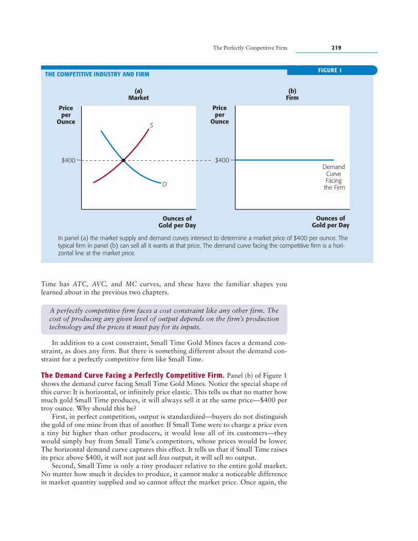
COST AND REVENUE DATA FOR A COMPETITIVE FIRMTable 1 shows cost and revenue data for Small Time. In the first two columns are dif-ferent quantities of gold that Small Time could produce each day and the maximum


In perfect competition, the firm is a price taker—it treats the price of its out-put as given.

Price taker Any firm that treats theprice of its product as given and be-yond its control.

COST AND REVENUE DATA FOR SMALL TIMEGOLD MINES

TABLE 1(1) (2)

Output Price (3) (4) (5) (6)(Troy Ounces of (per Troy Total Marginal Total Marginal (7)Gold per Day) Ounce) Revenue Revenue Cost Cost Profit

0 $400 $ 0 $ 550 �$550$400 $450

1 $400 $ 400 $1,000 �$600$400 $200

2 $400 $ 800 $1,200 �$400$400 $ 50

3 $400 $1,200 $1,250 �$ 50$400 $100

4 $400 $1,600 $1,350 $250$400 $150

5 $400 $2,000 $1,500 $500$400 $250

6 $400 $2,400 $1,750 $650$400 $350

7 $400 $2,800 $2,100 $700$400 $450

8 $400 $3,200 $2,550 $650$400 $550

9 $400 $3,600 $3,100 $500$400 $650

10 $400 $4,000 $3,750 $250

price that it could charge. Because Small Time is a competitive firm—a price taker—the price remains constant at $400 per ounce, no matter how much gold it produces.

Run your finger down the total revenue and marginal revenue columns. Sinceprice is always $400, each time the firm produces another ounce of gold, total rev-enue rises by $400. This is why marginal revenue—the additional revenue from sell-ing one more ounce of gold—remains constant at $400.

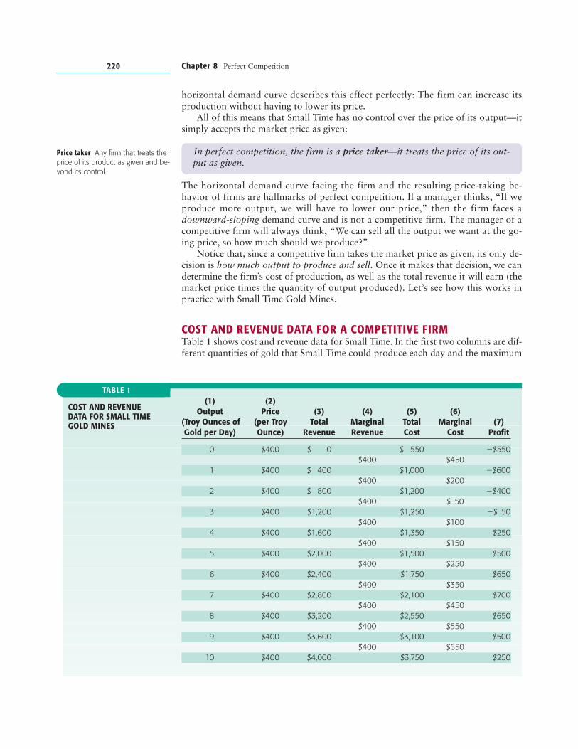
Figure 2 plots Small Time’s total revenue and marginal revenue. Notice that thetotal revenue (TR) curve in panel (a) is a straight line that slopes upward—eachtime output increases by one unit, TR rises by the same $400. That is, the slope ofthe TR curve is equal to the price of output.



TR

550

$2,800

2,100

(a)

TC

MaximumProfit

per Day= $700


Dollars

Dollars

MC

(b)

1 2 3 4 5 6 7 8 9 10

$400 d = MR

1 2

Slope = 400

3 4 5 6 7 8 9 10

Panel (a) shows a competi-tive firm’s total revenue (TR)and total cost (TC) curves.TR is a straight line withslope equal to the marketprice. Profit is maximized at7 ounces per day, where thevertical distance between TRand TC is greatest. Panel (b)shows that profit is maxi-mized where the marginalcost (MC) curve intersectsthe horizontal demand (d )and marginal revenue (MR)curves.

FIGURE 2PROFIT MAXIMIZATION IN PERFECT COMPETITION

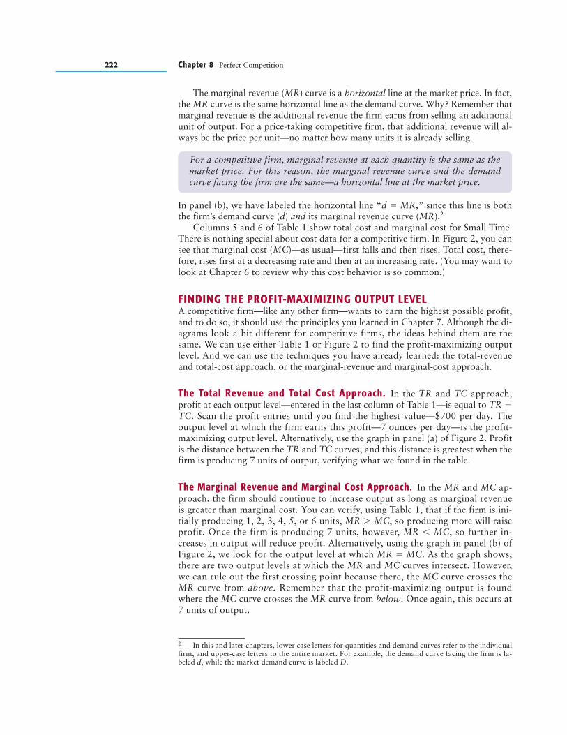
The marginal revenue (MR) curve is a horizontal line at the market price. In fact,the MR curve is the same horizontal line as the demand curve. Why? Remember thatmarginal revenue is the additional revenue the firm earns from selling an additionalunit of output. For a price-taking competitive firm, that additional revenue will al-ways be the price per unit—no matter how many units it is already selling.

In panel (b), we have labeled the horizontal line “d � MR,” since this line is boththe firm’s demand curve (d) and its marginal revenue curve (MR).2

Columns 5 and 6 of Table 1 show total cost and marginal cost for Small Time.There is nothing special about cost data for a competitive firm. In Figure 2, you cansee that marginal cost (MC)—as usual—first falls and then rises. Total cost, there-fore, rises first at a decreasing rate and then at an increasing rate. (You may want tolook at Chapter 6 to review why this cost behavior is so common.)

FINDING THE PROFIT-MAXIMIZING OUTPUT LEVELA competitive firm—like any other firm—wants to earn the highest possible profit,and to do so, it should use the principles you learned in Chapter 7. Although the di-agrams look a bit different for competitive firms, the ideas behind them are thesame. We can use either Table 1 or Figure 2 to find the profit-maximizing outputlevel. And we can use the techniques you have already learned: the total-revenueand total-cost approach, or the marginal-revenue and marginal-cost approach.

The Total Revenue and Total Cost Approach. In the TR and TC approach,profit at each output level—entered in the last column of Table 1—is equal to TR �TC. Scan the profit entries until you find the highest value—$700 per day. The output level at which the firm earns this profit—7 ounces per day—is the profit-maximizing output level. Alternatively, use the graph in panel (a) of Figure 2. Profitis the distance between the TR and TC curves, and this distance is greatest when thefirm is producing 7 units of output, verifying what we found in the table.

The Marginal Revenue and Marginal Cost Approach. In the MR and MC ap-proach, the firm should continue to increase output as long as marginal revenueis greater than marginal cost. You can verify, using Table 1, that if the firm is ini-tially producing 1, 2, 3, 4, 5, or 6 units, MR � MC, so producing more will raiseprofit. Once the firm is producing 7 units, however, MR � MC, so further in-creases in output will reduce profit. Alternatively, using the graph in panel (b) ofFigure 2, we look for the output level at which MR � MC. As the graph shows,there are two output levels at which the MR and MC curves intersect. However,we can rule out the first crossing point because there, the MC curve crosses theMR curve from above. Remember that the profit-maximizing output is foundwhere the MC curve crosses the MR curve from below. Once again, this occurs at7 units of output.


For a competitive firm, marginal revenue at each quantity is the same as themarket price. For this reason, the marginal revenue curve and the demandcurve facing the firm are the same—a horizontal line at the market price.

2 In this and later chapters, lower-case letters for quantities and demand curves refer to the individualfirm, and upper-case letters to the entire market. For example, the demand curve facing the firm is la-beled d, while the market demand curve is labeled D.


You can see that finding the profit-maximizing output level for a competitivefirm requires no new concepts or techniques; you have already learned everythingyou need to know in Chapter 7. In fact, the only difference is one of appearance.Ned’s Beds—our firm in Chapter 7—did not operate under perfect competition. Asa result, both its demand curve and its marginal revenue curve sloped downward.Small Time, however, operates under perfect competition, so its demand and MRcurves are the same horizontal line.

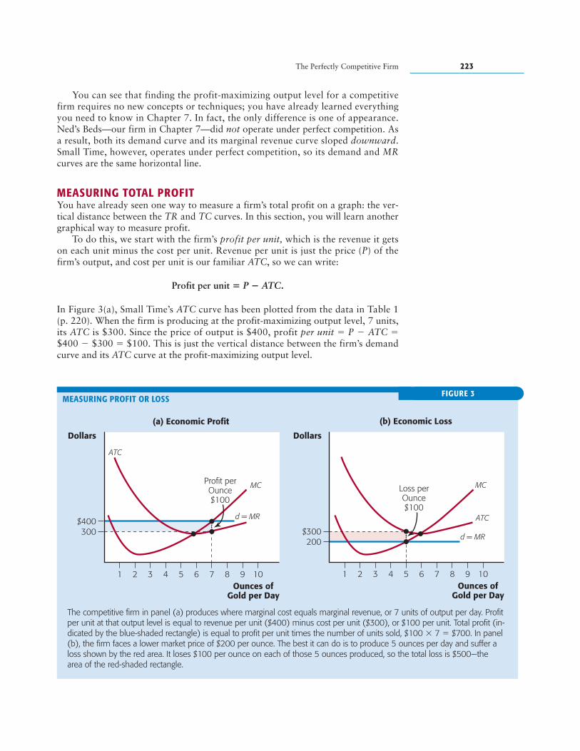
MEASURING TOTAL PROFITYou have already seen one way to measure a firm’s total profit on a graph: the ver-tical distance between the TR and TC curves. In this section, you will learn anothergraphical way to measure profit.

To do this, we start with the firm’s profit per unit, which is the revenue it getson each unit minus the cost per unit. Revenue per unit is just the price (P) of thefirm’s output, and cost per unit is our familiar ATC, so we can write:

Profit per unit � P � ATC.

In Figure 3(a), Small Time’s ATC curve has been plotted from the data in Table 1(p. 220). When the firm is producing at the profit-maximizing output level, 7 units,its ATC is $300. Since the price of output is $400, profit per unit � P � ATC �$400 � $300 � $100. This is just the vertical distance between the firm’s demandcurve and its ATC curve at the profit-maximizing output level.


Dollars

1 2 3 4 5 6 7 8 9 10

$400300

Profit perOunce$100

d = MR

MC

ATC

(a) Economic Profit


Dollars

MC

ATC

d = MR$300200

1 2 3 4 5 6 7 8 9 10

Loss perOunce$100

(b) Economic Loss

The competitive firm in panel (a) produces where marginal cost equals marginal revenue, or 7 units of output per day. Profitper unit at that output level is equal to revenue per unit ($400) minus cost per unit ($300), or $100 per unit. Total profit (in-dicated by the blue-shaded rectangle) is equal to profit per unit times the number of units sold, $100 � 7 � $700. In panel(b), the firm faces a lower market price of $200 per ounce. The best it can do is to produce 5 ounces per day and suffer aloss shown by the red area. It loses $100 per ounce on each of those 5 ounces produced, so the total loss is $500—thearea of the red-shaded rectangle.

FIGURE 3MEASURING PROFIT OR LOSS

Once we know Small Time’s profit per unit, it is easy to calculate its total profit:Just multiply profit per unit by the number of units sold. Small Time is earning$100 profit on each ounce of gold, and it sells 7 ounces in all, so total profit is $100� 7 � $700.

Now look at the blue-shaded rectangle in Figure 3(a). The height of this rectan-gle is profit per unit, and the width is the number of units produced. The area of therectangle—height � width—equals Small Time’s profit:

In the figure, Small Time is fortunate: At a price of $400, there are several outputlevels at which it can earn a profit. Its problem is to select the one that makes itsprofit as large as possible. (We should all have such problems.)

But what if the price had been lower than $400—so low, in fact, that SmallTime could not make a profit at any output level? Then the best it can do is tochoose the smallest possible loss. Just as we did in the case of profit, we can meas-ure the firm’s total loss using the ATC curve.

Panel (b) of Figure 3 reproduces Small Time’s ATC and MC curves from panel(a). This time, however, we have assumed a lower price for gold—$200—so thefirm’s d � MR curve is the horizontal line at $200. Since this line lies everywherebelow the ATC curve, profit per unit (P � ATC) is always negative: Small Time can-not make a positive profit at any output level.

With a price of $200, the MC curve crosses the MR curve from below at 5 unitsof output. Thus, unless Small Time decides to shut down (we’ll discuss shuttingdown later), it should produce 5 units. At that level of output, ATC is $300, andprofit per unit is P � ATC � $200 � $300 � �$100, a loss of $100 per unit. Thetotal loss is loss per unit times the number of units produced, or �$100 � 5 ��$500. This is equal to the area of the red-shaded rectangle in Figure 3(b), withheight equal to $100 and width equal to 5 units:

THE FIRM’S SHORT-RUN SUPPLY CURVEA competitive firm is a price taker: It takes the market price as given and then de-cides how much output it will produce at that price. If the market price changesfor any reason, the price taken as given will change as well. The firm will thenhave to find a new profit-maximizing output level. Let’s see how the firm’s choiceof output changes as the market price rises or falls.

Figure 4(a) shows ATC,AVC, and MC curves for a competitive producer ofwheat. The figure also showsfive hypothetical demandcurves the firm might face,each corresponding to a differ-ent market price for wheat. If


A firm earns a profit whenever P � ATC. Its total profit at the best outputlevel equals the area of a rectangle with height equal to the distance between Pand ATC, and width equal to the level of output.

It is tempting—but wrong—to think that the firm should produce where profitper unit (P � ATC) is greatest. The firm’s goal is to maximize total profit,not profit per unit. Using Table 1 or Figure 3(a), you can verify that while

Small Time’s profit per unit is greatest at 6 units of output, its total profit isgreatest at 7 units.

A firm suffers a loss whenever P � ATC at the best level of output. Its totalloss equals the area of a rectangle with height equal to the distance between Pand ATC, and width equal to the level of output.

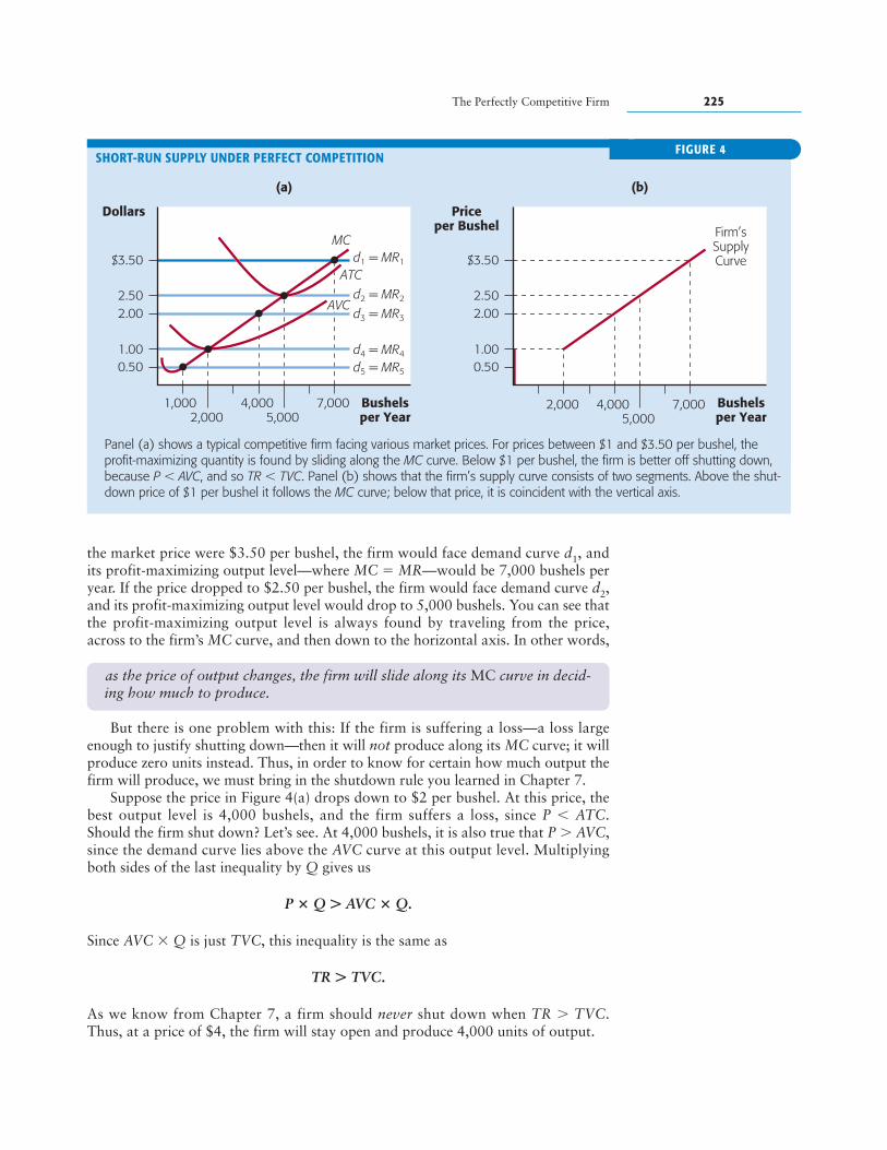
the market price were $3.50 per bushel, the firm would face demand curve d1, andits profit-maximizing output level—where MC � MR—would be 7,000 bushels peryear. If the price dropped to $2.50 per bushel, the firm would face demand curve d2,and its profit-maximizing output level would drop to 5,000 bushels. You can see thatthe profit-maximizing output level is always found by traveling from the price,across to the firm’s MC curve, and then down to the horizontal axis. In other words,

But there is one problem with this: If the firm is suffering a loss—a loss largeenough to justify shutting down—then it will not produce along its MC curve; it willproduce zero units instead. Thus, in order to know for certain how much output thefirm will produce, we must bring in the shutdown rule you learned in Chapter 7.

Suppose the price in Figure 4(a) drops down to $2 per bushel. At this price, thebest output level is 4,000 bushels, and the firm suffers a loss, since P � ATC.Should the firm shut down? Let’s see. At 4,000 bushels, it is also true that P � AVC,since the demand curve lies above the AVC curve at this output level. Multiplyingboth sides of the last inequality by Q gives us

P � Q � AVC � Q.

Since AVC � Q is just TVC, this inequality is the same as

TR � TVC.

As we know from Chapter 7, a firm should never shut down when TR � TVC.Thus, at a price of $4, the firm will stay open and produce 4,000 units of output.


Bushelsper Year

Dollars

0.50

1,0002,000

4,0005,000

7,000

1.00

2.00

$3.50

2.50 d2 = MR2

d3 = MR3

d4 = MR4

d5 = MR5

MC

ATCd1 = MR1

AVC

(a)

Firm’sSupplyCurve

Bushelsper Year

Priceper Bushel

0.50

2,000 4,0005,000

7,000

1.00

2.00

$3.50

2.50

(b)

Panel (a) shows a typical competitive firm facing various market prices. For prices between $1 and $3.50 per bushel, theprofit-maximizing quantity is found by sliding along the MC curve. Below $1 per bushel, the firm is better off shutting down,because P � AVC, and so TR � TVC. Panel (b) shows that the firm’s supply curve consists of two segments. Above the shut-down price of $1 per bushel it follows the MC curve; below that price, it is coincident with the vertical axis.

FIGURE 4SHORT-RUN SUPPLY UNDER PERFECT COMPETITION

as the price of output changes, the firm will slide along its MC curve in decid-ing how much to produce.

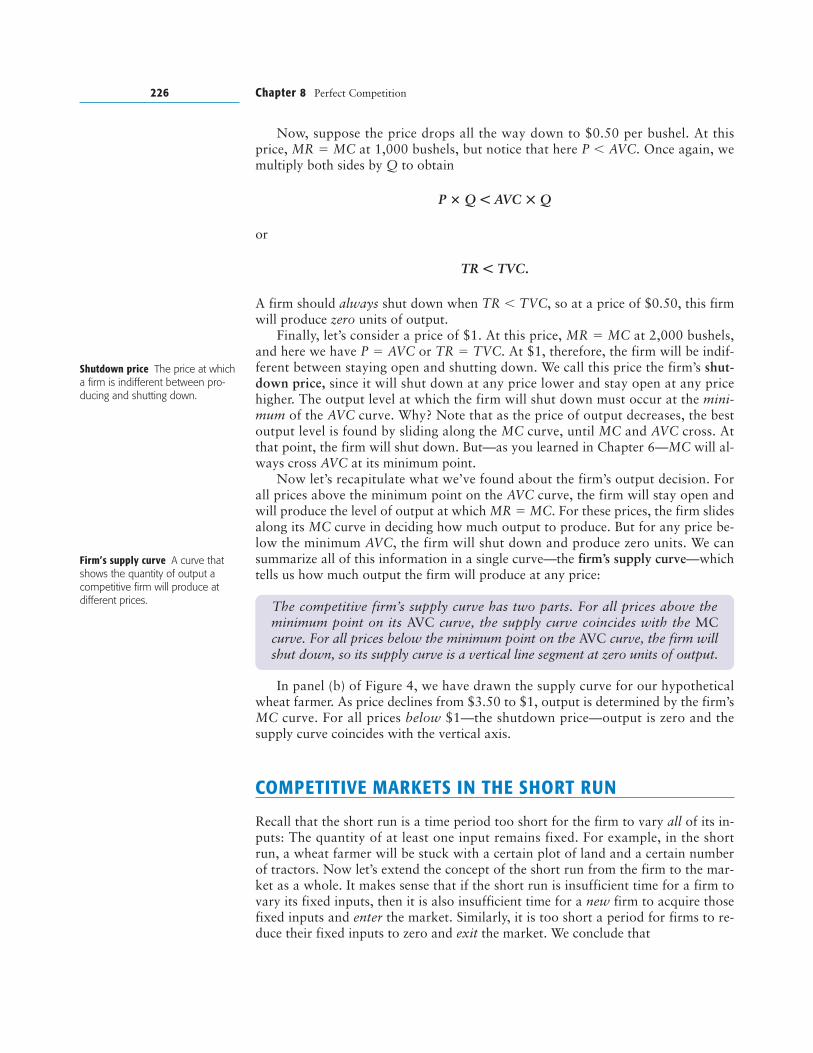
Now, suppose the price drops all the way down to $0.50 per bushel. At thisprice, MR � MC at 1,000 bushels, but notice that here P � AVC. Once again, wemultiply both sides by Q to obtain

P � Q � AVC � Q

or

TR � TVC.

A firm should always shut down when TR � TVC, so at a price of $0.50, this firmwill produce zero units of output.

Finally, let’s consider a price of $1. At this price, MR � MC at 2,000 bushels,and here we have P � AVC or TR � TVC. At $1, therefore, the firm will be indif-ferent between staying open and shutting down. We call this price the firm’s shut-down price, since it will shut down at any price lower and stay open at any pricehigher. The output level at which the firm will shut down must occur at the mini-mum of the AVC curve. Why? Note that as the price of output decreases, the bestoutput level is found by sliding along the MC curve, until MC and AVC cross. Atthat point, the firm will shut down. But—as you learned in Chapter 6—MC will al-ways cross AVC at its minimum point.

Now let’s recapitulate what we’ve found about the firm’s output decision. Forall prices above the minimum point on the AVC curve, the firm will stay open andwill produce the level of output at which MR � MC. For these prices, the firm slidesalong its MC curve in deciding how much output to produce. But for any price be-low the minimum AVC, the firm will shut down and produce zero units. We cansummarize all of this information in a single curve—the firm’s supply curve—whichtells us how much output the firm will produce at any price:

In panel (b) of Figure 4, we have drawn the supply curve for our hypotheticalwheat farmer. As price declines from $3.50 to $1, output is determined by the firm’sMC curve. For all prices below $1—the shutdown price—output is zero and thesupply curve coincides with the vertical axis.

COMPETITIVE MARKETS IN THE SHORT RUN

Recall that the short run is a time period too short for the firm to vary all of its in-puts: The quantity of at least one input remains fixed. For example, in the shortrun, a wheat farmer will be stuck with a certain plot of land and a certain numberof tractors. Now let’s extend the concept of the short run from the firm to the mar-ket as a whole. It makes sense that if the short run is insufficient time for a firm tovary its fixed inputs, then it is also insufficient time for a new firm to acquire thosefixed inputs and enter the market. Similarly, it is too short a period for firms to re-duce their fixed inputs to zero and exit the market. We conclude that


Shutdown price The price at whicha firm is indifferent between pro-ducing and shutting down.

Firm’s supply curve A curve thatshows the quantity of output acompetitive firm will produce atdifferent prices. The competitive firm’s supply curve has two parts. For all prices above the

minimum point on its AVC curve, the supply curve coincides with the MCcurve. For all prices below the minimum point on the AVC curve, the firm willshut down, so its supply curve is a vertical line segment at zero units of output.

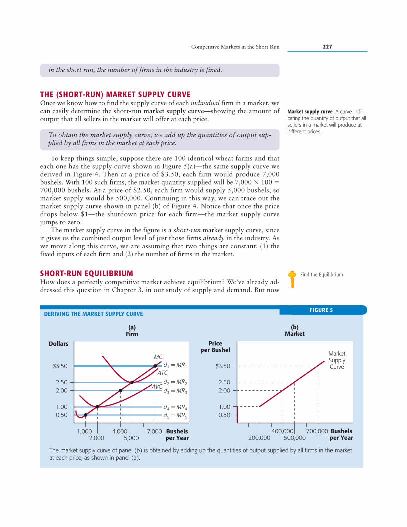
THE (SHORT-RUN) MARKET SUPPLY CURVEOnce we know how to find the supply curve of each individual firm in a market, wecan easily determine the short-run market supply curve—showing the amount ofoutput that all sellers in the market will offer at each price.

To keep things simple, suppose there are 100 identical wheat farms and thateach one has the supply curve shown in Figure 5(a)—the same supply curve wederived in Figure 4. Then at a price of $3.50, each firm would produce 7,000bushels. With 100 such firms, the market quantity supplied will be 7,000 � 100 �700,000 bushels. At a price of $2.50, each firm would supply 5,000 bushels, somarket supply would be 500,000. Continuing in this way, we can trace out themarket supply curve shown in panel (b) of Figure 4. Notice that once the pricedrops below $1—the shutdown price for each firm—the market supply curvejumps to zero.

The market supply curve in the figure is a short-run market supply curve, sinceit gives us the combined output level of just those firms already in the industry. Aswe move along this curve, we are assuming that two things are constant: (1) thefixed inputs of each firm and (2) the number of firms in the market.

SHORT-RUN EQUILIBRIUMHow does a perfectly competitive market achieve equilibrium? We’ve already ad-dressed this question in Chapter 3, in our study of supply and demand. But now

Competitive Markets in the Short Run 227

in the short run, the number of firms in the industry is fixed.

Market supply curve A curve indi-cating the quantity of output that allsellers in a market will produce atdifferent prices.To obtain the market supply curve, we add up the quantities of output sup-

plied by all firms in the market at each price.

Bushelsper Year

Dollars

0.50

1,0002,000

4,0005,000

7,000

1.00

2.00

$3.50

2.50

0.501.00

2.00

$3.50

2.50d2 = MR2

d3 = MR3

d4 = MR4

d5 = MR5

MC

ATCd1 = MR1

AVC

(a)Firm

MarketSupplyCurve

Bushelsper Year

Priceper Bushel

200,000400,000

500,000700,000

(b)Market

The market supply curve of panel (b) is obtained by adding up the quantities of output supplied by all firms in the marketat each price, as shown in panel (a).

FIGURE 5DERIVING THE MARKET SUPPLY CURVE

Find the Equilibrium

we’ll take a much closer look, paying attention to the individual firm and individ-ual consumer as well as the market.

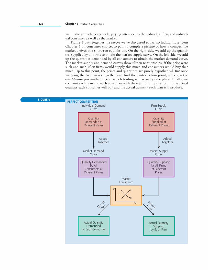
Figure 6 puts together the pieces we’ve discussed so far, including those fromChapter 5 on consumer choice, to paint a complete picture of how a competitivemarket arrives at a short-run equilibrium. On the right side, we add up the quanti-ties supplied by all firms to obtain the market supply curve. On the left side, we addup the quantities demanded by all consumers to obtain the market demand curve.The market supply and demand curves show if/then relationships: If the price weresuch and such, then firms would supply this much and consumers would buy thatmuch. Up to this point, the prices and quantities are purely hypothetical. But oncewe bring the two curves together and find their intersection point, we know theequilibrium price—the price at which trading will actually take place. Finally, weconfront each firm and each consumer with the equilibrium price to find the actualquantity each consumer will buy and the actual quantity each firm will produce.


Individual DemandCurve

QuantityDemanded atDifferent Prices

Market DemandCurve

Quantity Demandedby All

Consumers atDifferent Prices

Firm SupplyCurve

QuantitySupplied at

Different Prices

Market SupplyCurve

Quantity Suppliedby All Firmsat Different

Prices

AddedTogether

MarketEquilibrium

P

Q

S

D

Actual QuantityDemanded

by Each Consumer

Actual QuantitySupplied

by Each Firm

Market

Price

MarketPrice

AddedTogether

FIGURE 6PERFECT COMPETITION

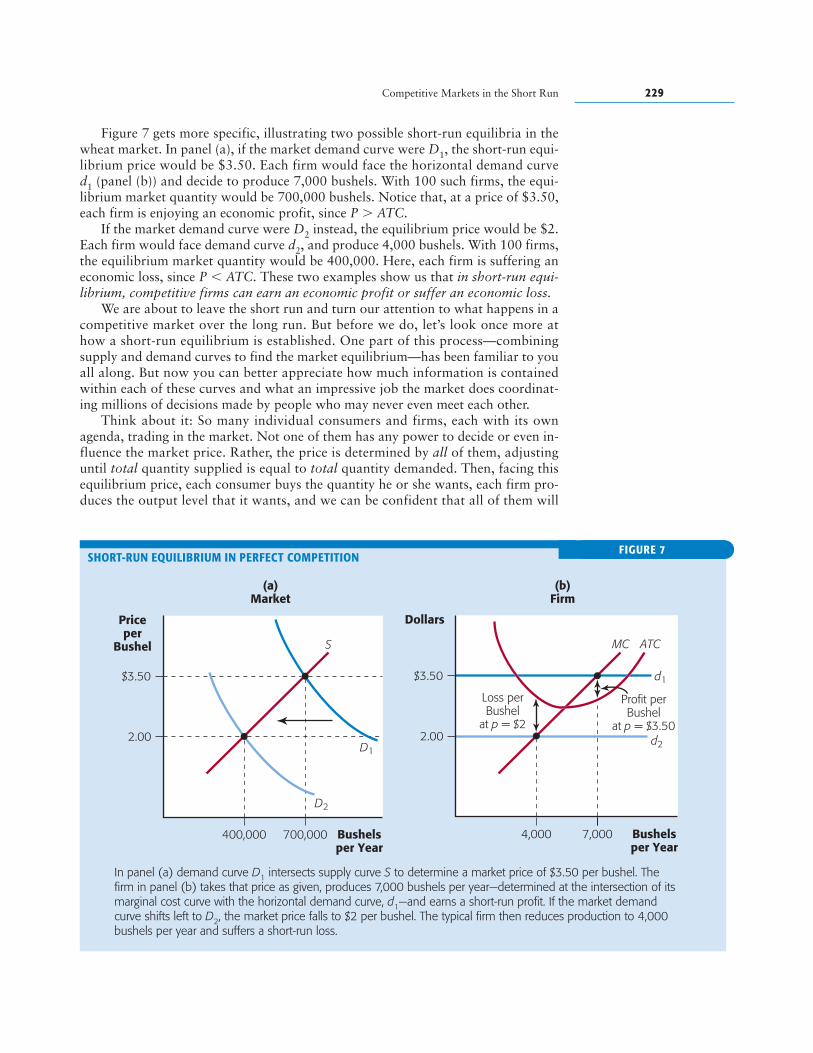
Figure 7 gets more specific, illustrating two possible short-run equilibria in thewheat market. In panel (a), if the market demand curve were D1, the short-run equi-librium price would be $3.50. Each firm would face the horizontal demand curved1 (panel (b)) and decide to produce 7,000 bushels. With 100 such firms, the equi-librium market quantity would be 700,000 bushels. Notice that, at a price of $3.50,each firm is enjoying an economic profit, since P � ATC.

If the market demand curve were D2 instead, the equilibrium price would be $2.Each firm would face demand curve d2, and produce 4,000 bushels. With 100 firms,the equilibrium market quantity would be 400,000. Here, each firm is suffering aneconomic loss, since P � ATC. These two examples show us that in short-run equi-librium, competitive firms can earn an economic profit or suffer an economic loss.

We are about to leave the short run and turn our attention to what happens in acompetitive market over the long run. But before we do, let’s look once more athow a short-run equilibrium is established. One part of this process—combiningsupply and demand curves to find the market equilibrium—has been familiar to youall along. But now you can better appreciate how much information is containedwithin each of these curves and what an impressive job the market does coordinat-ing millions of decisions made by people who may never even meet each other.

Think about it: So many individual consumers and firms, each with its ownagenda, trading in the market. Not one of them has any power to decide or even in-fluence the market price. Rather, the price is determined by all of them, adjustinguntil total quantity supplied is equal to total quantity demanded. Then, facing thisequilibrium price, each consumer buys the quantity he or she wants, each firm pro-duces the output level that it wants, and we can be confident that all of them will

Competitive Markets in the Short Run 229

Bushelsper Year

Priceper

Bushel

400,000 700,000

2.00

$3.50

S

D1

D2

(a)Market

MC

d1

d2

Loss perBushel

at p = $2

Profit perBushel

at p = $3.50

ATC

7,0004,000 Bushelsper Year

Dollars

2.00

$3.50

(b)Firm

In panel (a) demand curve D1 intersects supply curve S to determine a market price of $3.50 per bushel. Thefirm in panel (b) takes that price as given, produces 7,000 bushels per year—determined at the intersection of itsmarginal cost curve with the horizontal demand curve, d1—and earns a short-run profit. If the market demandcurve shifts left to D2, the market price falls to $2 per bushel. The typical firm then reduces production to 4,000bushels per year and suffers a short-run loss.

FIGURE 7SHORT-RUN EQUILIBRIUM IN PERFECT COMPETITION

be able to realize their plans. Each buyer can find willing sellers, and each seller canfind willing buyers.

This process is, from a certain perspective, a thing of beauty, and it happens eachday in markets all across the world—markets for wheat, corn, barley, soybeans, ap-ples, oranges, gold, silver, copper, and more. And something quite similar happensin other markets that do not strictly satisfy our requirements for perfect competi-tion—markets for television sets, books, air conditioners, fast-food meals, oil, natu-ral gas, bottled water, blue jeans. The list is virtually endless.

COMPETITIVE MARKETS IN THE LONG RUN

So far, we’ve explored the short run only, and assumed that the number of firms inthe market is fixed. But perfect competition becomes even more interesting in thelong run, when entry and exit can occur. After all, the long run is a time horizonlong enough for firms to vary all of their inputs. It should therefore be long enoughfor new firms to acquire fixed inputs and enter the market, and for firms already inthe industry to sell off their fixed inputs and exit from the market.

But what makes firms want to enter or exit a market? The driving force behindentry is economic profit, and the force behind exit is economic loss.

PROFIT AND LOSS AND THE LONG RUNRecall that economic profit is the amount by which total revenue exceeds all costs ofdoing business. The costs to be deducted include implicit costs like foregone invest-ment income and foregone wages for an owner who devotes money and time to thebusiness. Thus, when a firm earns positive economic profit, we know the owners areearning more than they could by devoting their money and time to some other activity.

A temporary episode of positive economic profit will not have much impact ona competitive industry, other than the temporary pleasure it gives the owners ofcompetitive firms. But when positive profit reflects basic conditions in the industryand is expected to continue, major changes are in the works. Outsiders, hungry forprofit themselves, will want to enter the market, and—since there are no barriers toentry—they can do so.

Similarly, if firms in the market are suffering economic losses, they are not earn-ing enough revenue to cover all their costs, so there must be other opportunities thatwould more adequately compensate owners for their money or time. If this situa-tion is expected to continue over the firm’s long-run planning horizon—a periodlong enough to vary all inputs—there is only one thing for the firm to do: exit themarket by selling off its plant and equipment, thereby reducing its loss to zero.


In perfect competition, the market sums up the buying and selling preferencesof individual consumers and producers, and determines the market price.Each buyer and seller then takes the market price as given, and each is able tobuy or sell the desired quantity.

In a competitive market, economic profit and loss are the forces driving long-run change. The expectation of continued economic profit causes outsiders toenter the market; the expectation of continued economic losses causes firms inthe market to exit.

Rocky Mountain Internet Service isone of more than 7,000 new Inter-net Service Providers that have en-tered the market due to high prof-its of existing firms.

In the real world of business, entry and exit occur literally every day. In somecases, we see entry occur through the formation of an entirely new firm. For exam-ple, in the late 1990s, the high profits of the earliest Internet service providers(ISPs)—such as America Online, CompuServe, and Prodigy—led to the establish-ment of more than 7,000 new ISPs by the end of the decade. Entry can also occurwhen an existing firm adds a new product to its line. For example, among the firmsthat entered the ISP market were many firms that had been established years beforethere was such as thing as an ISP, such as Sprint (which entered with Earthlink), Mi-crosoft (the Microsoft Network), and AT&T. Although these were not new firms,they were new participants in the market for Internet service.

Exit, too, can occur in different ways. A firm may go out of business entirely,selling off its assets and freeing itself once and for all from all costs. Every year,thousands of small businesses exit markets in this way. You may know of a localvideo store, grocery store, or furniture shop that decided to permanently shut itsdoors. Restaurants, in particular, seem especially prone to long-run economic loss.It has been reported that half of all new restaurants exit the market within twoyears of being established.

But exit can also occur when a firm switches out of a particular product line,even as it continues to produce other things. For example, publishing companies of-ten decide to abandon unsuccessful magazines, yet they continue to thrive by pub-lishing other magazines and books.

LONG-RUN EQUILIBRIUMEntry and exit—however they occur—are powerful forces in real-world competitivemarkets. They determine how these markets change over the long run, how muchoutput will ultimately be available to consumers, and the prices they must pay. Toexplore these issues, let’s see how entry and exit move a market to its long-run equi-librium from different starting points.

From Short-Run Profit to Long-Run Equilibrium. Suppose that the market forwheat is initially in a short-run equilibrium like point A in panel (a) of Figure 8, withmarket supply curve S1. The initial equilibrium price is $4.50 per bushel. In panel(b), we see that a typical competitive firm—producing 9,000 bushels—is earning eco-nomic profit, since P � ATC at that output level. As long as we remain in the shortrun—with no new firms entering the market—this situation will not change.

But as we enter the long run, much will change. First, economic profit will attractnew entrants, increasing the number of sellers in the market and shifting the marketsupply curve rightward. (Remember, the market supply curve S1 is drawn for a fixednumber of firms; with more firms in the market, a greater quantity will be supplied ateach price.) As the market supply curve shifts rightward, several things happen:

1. The market price begins to fall—from $4.50 to $4.00 to $3.50 and so on.2. As market price falls, the demand curve facing each firm shifts downward.3. Each firm—striving as always to maximize profit—will slide down its marginal

cost curve, decreasing output.3

This process of adjustment—in the market and the firm—continues until . . .well, until when? To answer this question, remember why these adjustments are

Competitive Markets in the Long Run 231

3 There is one other possible consequence that we ignore here: Entry into the industry—whichchanges the demand for the industry’s inputs—may also change input prices. If this occurs, firms’ ATCcurves will shift. For now, we will assume that entry (and exit) do not affect input prices, so that the ATCcurve does not shift.

Find the Equilibrium

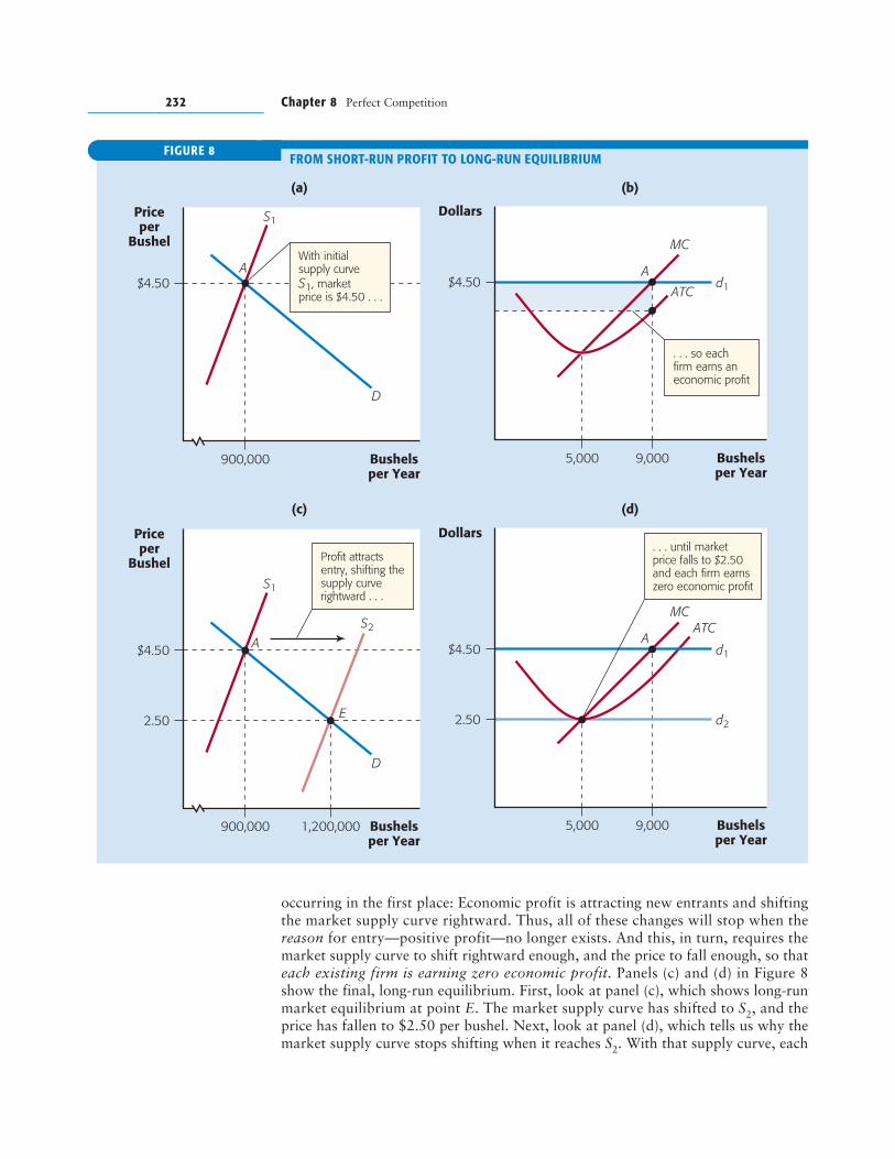
occurring in the first place: Economic profit is attracting new entrants and shiftingthe market supply curve rightward. Thus, all of these changes will stop when thereason for entry—positive profit—no longer exists. And this, in turn, requires themarket supply curve to shift rightward enough, and the price to fall enough, so thateach existing firm is earning zero economic profit. Panels (c) and (d) in Figure 8show the final, long-run equilibrium. First, look at panel (c), which shows long-runmarket equilibrium at point E. The market supply curve has shifted to S2, and theprice has fallen to $2.50 per bushel. Next, look at panel (d), which tells us why themarket supply curve stops shifting when it reaches S2. With that supply curve, each


Bushelsper Year

Priceper

Bushel

S1

D

A

900,000

$4.50A

d1

Bushelsper Year

Dollars

9,000

$4.50ATC

MC

Bushelsper Year

Priceper

Bushel

(c) (d)

(a) (b)

1,200,000

2.50

S1

D

A

E

S2

900,000

$4.50A

d1

d2

Bushelsper Year

Dollars

5,000

5,000

9,000

2.50

$4.50

ATCMC

With initialsupply curveS1, marketprice is $4.50 . . .

Profit attractsentry, shifting thesupply curverightward . . .

. . . until marketprice falls to $2.50and each firm earnszero economic profit

. . . so eachfirm earns an economic profit

FIGURE 8FROM SHORT-RUN PROFIT TO LONG-RUN EQUILIBRIUM

firm is producing at the lowest point of its ATC curve, with P � ATC � $2.50, andeach is earning zero economic profit. With no economic profit, there is no furtherreason for entry, and no further shift in the market supply curve.

Before proceeding further, take a close look at Figure 8. As the market moves toits long-run equilibrium (point E in panels (c) and (d)), output at each firm de-creases from 9,000 to 5,000 bushels. But in the market as a whole, output increasesfrom 900,000 to 1,200,000 bushels. How can this be? (See if you can answer thisquestion yourself. Hint: entry!)

From Short-Run Loss to Long-Run Equilibrium. We have just seen how, begin-ning from a position of short-run profit at the typical firm, a competitive marketwill adjust until the profit is eliminated. But what if we begin from a position ofloss? As you might guess, the same type of adjustments will occur, only in the oppo-site direction.

This is a good opportunity for you to test your own skill and understanding.Study Figure 8 carefully. Then see if you can draw a similar diagram that illustratesthe adjustment from short-run loss to long-run equilibrium. Start with a marketprice of $1. Use the same demand curve as in Figure 8, but draw in a new, appro-priate market supply curve. Then let the market work. Show what happens in themarket, and at each firm, as economic loss causes some firms to exit. If you do thiscorrectly, you’ll end up once again at a market price of $2.50, with each firm earn-ing zero economic profit. Your graph will illustrate the following conclusion:

Distinguishing Short-Run from Long-Run Outcomes. You’ve seen that theequilibrium in a competitive market can be very different in the short run than inthe long run. In short-run equilibrium, competitive firms can earn profits or sufferlosses. But in long-run equilibrium, after entry or exit has occurred, economic profitis always zero. The distinction between short-run and long-run equilibrium is im-portant, and not just in competitive markets. In any market, our analysis will de-pend on the time period we are considering, and the correct period depends on thequestion we are asking. If we want to predict what happens several years after achange in demand, we should ask what the new long-run equilibrium will be. If wewant to know what happens a few months after a change in demand, we’ll look forthe new short-run equilibrium.

When economists look at a market, they automatically think of the short runversus the long run and then choose the period more appropriate for the questionat hand. As you’ll see, this way of thinking is applied again and again in economics.

THE NOTION OF ZERO PROFIT IN PERFECT COMPETITIONFrom the preceding description, you may wonder why anyone in his or her rightmind would ever want to set up shop in a competitive industry or stay there for anylength of time, since—in the long run—they can expect zero economic profit. In-deed, if you want to become a millionaire, you would be well advised not to buy a


In a competitive market, positive economic profit continues to attract new en-trants until economic profit is reduced to zero.

In a competitive market, economic losses continue to cause exit until thelosses are reduced to zero.

wheat farm. But most wheat farmers—like most other sellers in competitive mar-kets—do not curse their fate. On the contrary, they are likely to be quite contentwith the performance of their businesses. How can this be?

Remember that zero economic profit is not the same as zero accountingprofit. When a firm is making zero economic profit, it is still making some ac-counting profit. In fact, the accounting profit is just enough to cover all of theowner’s costs—including compensation for any foregone investment income orforegone salary. Suppose, for example, that a wheat farmer paid $100,000 forland and works 40 hours per week. Suppose, too, that the money could have beeninvested in some other way and earned $6,000 per year, and the farmer couldhave worked equally pleasantly elsewhere and earned $40,000 per year. Then thefarm’s implicit costs will be $46,000, and zero economic profit would mean thatthe farm was earning $46,000 in accounting profit each year. This won’t make awheat farmer ecstatic, but it will make it worthwhile to keep working the farm.After all, if the farmer quits and takes up the next best alternative, he or she willdo no better. To emphasize that zero economic profit is not an unpleasant out-come, economists often replace it with the term normal profit, which is a syn-onym for “zero economic profit,” or “just enough accounting profit to cover im-plicit costs.” Using this language, we can summarize long-run conditions at thetypical firm this way:

PERFECT COMPETITION AND PLANT SIZEThere is one more characteristic of competitive markets in the long run that wehave not yet discussed: the plant size of the competitive firm. It turns out that thesame forces—entry and exit—that cause all firms to earn zero economic profitalso ensure that:

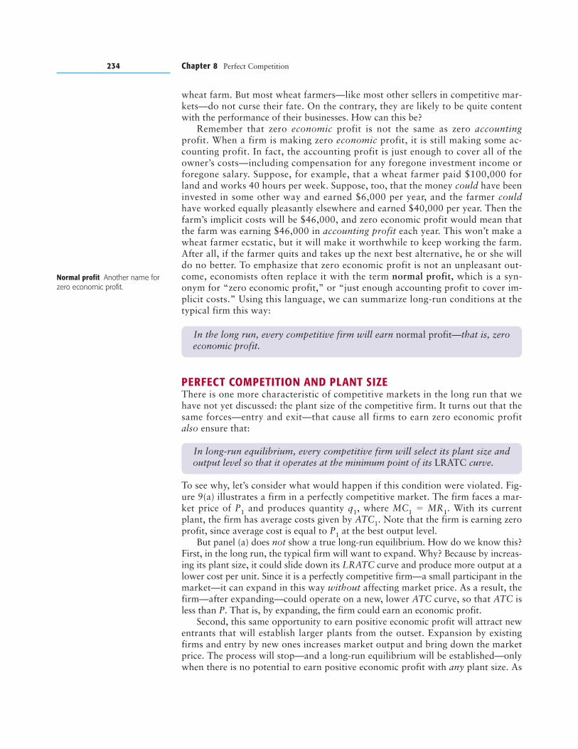
To see why, let’s consider what would happen if this condition were violated. Fig-ure 9(a) illustrates a firm in a perfectly competitive market. The firm faces a mar-ket price of P1 and produces quantity q1, where MC1 � MR1. With its currentplant, the firm has average costs given by ATC1. Note that the firm is earning zeroprofit, since average cost is equal to P1 at the best output level.

But panel (a) does not show a true long-run equilibrium. How do we know this?First, in the long run, the typical firm will want to expand. Why? Because by increas-ing its plant size, it could slide down its LRATC curve and produce more output at alower cost per unit. Since it is a perfectly competitive firm—a small participant in themarket—it can expand in this way without affecting market price. As a result, thefirm—after expanding—could operate on a new, lower ATC curve, so that ATC isless than P. That is, by expanding, the firm could earn an economic profit.

Second, this same opportunity to earn positive economic profit will attract newentrants that will establish larger plants from the outset. Expansion by existingfirms and entry by new ones increases market output and bring down the marketprice. The process will stop—and a long-run equilibrium will be established—onlywhen there is no potential to earn positive economic profit with any plant size. As


In the long run, every competitive firm will earn normal profit—that is, zeroeconomic profit.

In long-run equilibrium, every competitive firm will select its plant size andoutput level so that it operates at the minimum point of its LRATC curve.

Normal profit Another name forzero economic profit.

you can see in panel (b), this condition is satisfied only when each firm is operatingat the minimum point on its LRATC curve, using the plant represented by ATC2,and producing output of q*. Entry and expansion must continue in this market un-til the price falls to P*, because only then will each firm—doing the best that it cando—earn zero economic profit. (Question: In the long run, what would happen tothe firm in panel (a) if it refused to increase its plant size?)

A SUMMARY OF THE COMPETITIVE FIRM IN THE LONG RUNPanel (b) of Figure 9 summarizes everything you have learned about the competi-tive firm in long-run equilibrium. The typical firm—taking the market price P* asgiven—produces the profit-maximizing output level q*, where MR � MC. Sincethis is the long run, each firm will be earning zero economic profit, so we also knowthat P* � ATC. But since P* � MC and P* � ATC, it must also be true that MC �ATC. As you learned in Chapter 6, MC and ATC are equal only at the minimumpoint of the ATC curve. Thus, we know that each firm must be operating at thelowest possible point on the ATC curve for the plant it is operating. Finally, eachfirm selects the plant that makes its LRATC as low as possible, so each operates atthe minimum point on its LRATC curve.

As you can see, there is a lot going on in Figure 9 (b). But we can put it all to-gether with a very simple statement:


Outputper

Period

Dollars

P1

(a)

q1

d1 = MR1

LRATCMC1 ATC1

Dollars

(b)

E

Outputper

Period

d2 = MR2

LRATC

MC2 ATC2

P*

q*

The firm in panel (a) faces a price of P1 and produces quantity q1. It earns zero profit because price equals average cost.In the long run, this firm will want to expand. By sliding down LRATC, it could produce more output at a lower cost perunit and earn an economic profit. In turn, economic profit will attract entry, and that will reduce the market price. Thefirm’s long-run equilibrium position is shown in panel (b). The firm earns zero profit by operating at minimum LRATC.

FIGURE 9PERFECT COMPETITION AND PLANT SIZE

At each competitive firm in long-run equilibrium, P � MC � minimum ATC� minimum LRATC.

In Figure 9(b), this equality is satisfied when the typical firm produces at pointE, where its demand, marginal cost, ATC, and LRATC curves all intersect. This is afigure well worth remembering, since it summarizes so much information aboutcompetitive markets in a single picture. (Here is a useful self-test: Close the book,put away your notes, and draw a set of diagrams in which one curve at a time doesnot pass through the common intersection point of the other three. Then explainwhich principle of firm or market behavior is violated by your diagram. Do this sep-arately for all four curves.)

Figure 9(b) also explains one of the important ways in which perfect competi-tion benefits consumers: In the long run, each firm is driven to the plant size andoutput level at which its cost per unit is as low as possible. This lowest possiblecost per unit is also the price per unit that consumers will pay. If price were anylower than P*, it would not be worthwhile for firms to continue producing thegood in the long run. Thus, given the ATC curve faced by each firm in this indus-try—a curve that is determined by each firm’s production technology and the costsof its inputs—P* is the lowest possible price that will ensure the continued avail-ability of the good. In perfect competition, consumers are getting the best deal theycould possibly get.

WHAT HAPPENS WHEN THINGS CHANGE?

So far, you’ve learned how competitive firms make decisions, how these decisionslead to a short-run equilibrium in the market, and how the market moves fromshort- to long-run equilibrium through entry and exit. Now, it’s time to turn to KeyStep 4: What happens when things change? In this section, we’ll deal with a changein demand for the product and, in the process, learn some important additional fea-tures of perfect competition. In the section titled “Using the Theory,” we’ll look atchanges in technology.

A CHANGE IN DEMANDIn Figure 10, panel (a) shows a competitive market that is initially in long-run equi-librium at point A, where the market demand curve D1 and supply curve S1 inter-sect. (Ignore the other curves for now). Panel (b) shows conditions at the firm,which faces demand curve d1 and produces the profit-maximizing quantity q1.

But now suppose that the market demand curve shifts rightward to D2 and re-mains there. (This shift could be caused by any one of several factors. If you can’tlist some of them, turn back to Chapter 3 and look again at Figure 3.) Panels (c) and(d) show what happens. In the short run, the shift in demand moves the marketequilibrium to point B, with market output QSR and price PSR. At the same time,the demand curve facing each firm shifts upward, and each firm raises output to thenew profit-maximizing level qSR. At this output level, P � ATC, so each firm isearning economic profit. Thus, the short-run impact of an increase in demand is (1) a rise in market price, (2) a rise in market quantity, and (3) economic profits.

When we turn to the long run, we know that entry will occur (why?), so themarket supply curve shifts rightward, bringing down the price until each firm earnszero economic profit. But how far must the price fall in order to bring this about?That is, how far can we expect the market supply curve to shift? In answering thisquestion, we’ll add one more detail to our model that we’ve ignored until now.

Think about what happens as entry occurs in an industry. With more firms,output increases, so the industry will demand more inputs—more raw materials,


Economists have tried to simu-late the behavior of competitivemarkets through experiments.Vanderbilt University’s Market.Econ is an Internet-basedexample (http://market.econ.vanderbilt.edu).

http://

What Happens When Things Change?

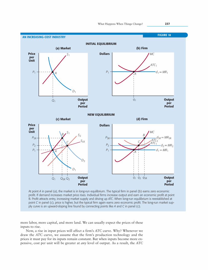
more labor, more capital, and more land. We can usually expect the prices of theseinputs to rise.

Now, a rise in input prices will affect a firm’s ATC curve. Why? Whenever wedraw the ATC curve, we assume that the firm’s production technology and theprices it must pay for its inputs remain constant. But when inputs become more ex-pensive, cost per unit will be greater at any level of output. As a result, the ATC

What Happens When Things Change? 237

Outputper

Period

PriceperUnit

D1

S1S2

SLR

B

A

C

P1

P2

PSR

Q1 QSR Q2

D2

(c) Market

Dollars

(d) FirmNEW EQUILIBRIUM

INITIAL EQUILIBRIUM

Outputper

Period

P1

P2

PSR

q1 qSRq2

BMC

C

A

dSR = MRSR

d2 = MR2

ATC2ATC1

d1 = MR1

Outputper

Period

PriceperUnit

D1

S1

AP1

Q1

(a) Market

Dollars

(b) Firm

Outputper

Period

P1

q1

MC

A

ATC1

d1 = MR1

At point A in panel (a), the market is in long-run equilibrium. The typical firm in panel (b) earns zero economicprofit. If demand increases market price rises. Individual firms increase output and earn an economic profit at pointB. Profit attracts entry, increasing market supply and driving up ATC. When long-run equilibrium is reestablished atpoint C in panel (c), price is higher, but the typical firm again earns zero economic profit. The long-run market sup-ply curve is an upward-sloping line found by connecting points like A and C in panel (c).

FIGURE 10AN INCREASING-COST INDUSTRY

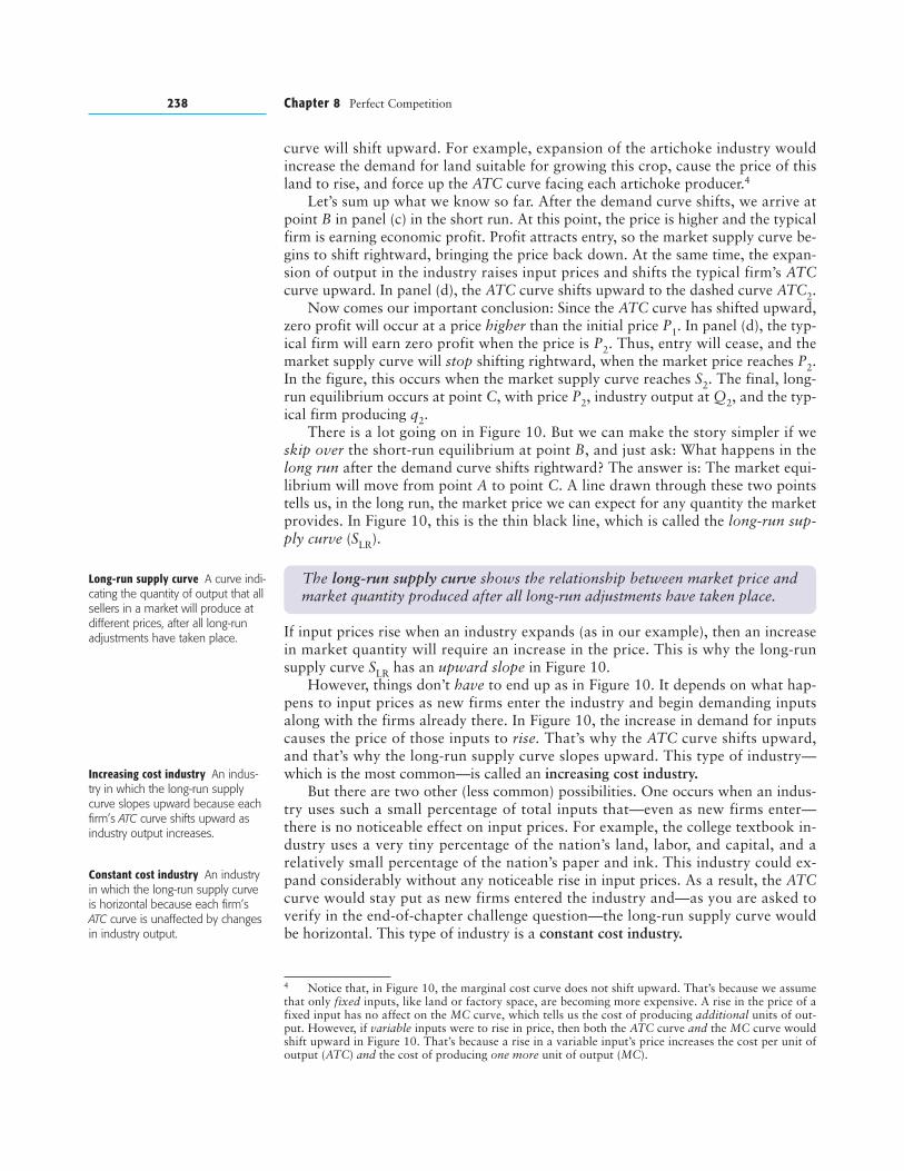
curve will shift upward. For example, expansion of the artichoke industry wouldincrease the demand for land suitable for growing this crop, cause the price of thisland to rise, and force up the ATC curve facing each artichoke producer.4

Let’s sum up what we know so far. After the demand curve shifts, we arrive atpoint B in panel (c) in the short run. At this point, the price is higher and the typicalfirm is earning economic profit. Profit attracts entry, so the market supply curve be-gins to shift rightward, bringing the price back down. At the same time, the expan-sion of output in the industry raises input prices and shifts the typical firm’s ATCcurve upward. In panel (d), the ATC curve shifts upward to the dashed curve ATC2.

Now comes our important conclusion: Since the ATC curve has shifted upward,zero profit will occur at a price higher than the initial price P1. In panel (d), the typ-ical firm will earn zero profit when the price is P2. Thus, entry will cease, and themarket supply curve will stop shifting rightward, when the market price reaches P2.In the figure, this occurs when the market supply curve reaches S2. The final, long-run equilibrium occurs at point C, with price P2, industry output at Q2, and the typ-ical firm producing q2.

There is a lot going on in Figure 10. But we can make the story simpler if weskip over the short-run equilibrium at point B, and just ask: What happens in thelong run after the demand curve shifts rightward? The answer is: The market equi-librium will move from point A to point C. A line drawn through these two pointstells us, in the long run, the market price we can expect for any quantity the marketprovides. In Figure 10, this is the thin black line, which is called the long-run sup-ply curve (SLR).

If input prices rise when an industry expands (as in our example), then an increasein market quantity will require an increase in the price. This is why the long-runsupply curve SLR has an upward slope in Figure 10.

However, things don’t have to end up as in Figure 10. It depends on what hap-pens to input prices as new firms enter the industry and begin demanding inputsalong with the firms already there. In Figure 10, the increase in demand for inputscauses the price of those inputs to rise. That’s why the ATC curve shifts upward,and that’s why the long-run supply curve slopes upward. This type of industry—which is the most common—is called an increasing cost industry.

But there are two other (less common) possibilities. One occurs when an indus-try uses such a small percentage of total inputs that—even as new firms enter—there is no noticeable effect on input prices. For example, the college textbook in-dustry uses a very tiny percentage of the nation’s land, labor, and capital, and arelatively small percentage of the nation’s paper and ink. This industry could ex-pand considerably without any noticeable rise in input prices. As a result, the ATCcurve would stay put as new firms entered the industry and—as you are asked toverify in the end-of-chapter challenge question—the long-run supply curve wouldbe horizontal. This type of industry is a constant cost industry.


The long-run supply curve shows the relationship between market price andmarket quantity produced after all long-run adjustments have taken place.

Long-run supply curve A curve indi-cating the quantity of output that allsellers in a market will produce atdifferent prices, after all long-runadjustments have taken place.

Increasing cost industry An indus-try in which the long-run supplycurve slopes upward because eachfirm’s ATC curve shifts upward asindustry output increases.

Constant cost industry An industryin which the long-run supply curveis horizontal because each firm’sATC curve is unaffected by changesin industry output.

4 Notice that, in Figure 10, the marginal cost curve does not shift upward. That’s because we assumethat only fixed inputs, like land or factory space, are becoming more expensive. A rise in the price of afixed input has no affect on the MC curve, which tells us the cost of producing additional units of out-put. However, if variable inputs were to rise in price, then both the ATC curve and the MC curve wouldshift upward in Figure 10. That’s because a rise in a variable input’s price increases the cost per unit ofoutput (ATC) and the cost of producing one more unit of output (MC).

The last possibility is that of a decreasing cost industry, in which entry by newfirms actually decreases input prices. This will occur when firms that make the in-puts experience economies of scale, so that their cost per unit—and the prices theycharge—come down as they step up production. For example, videotapes are an im-portant input for video rental stores. In the 1980s, the entry of new firms into thevideo rental industry led to increased demand for, and production of, videotapes.But since videotape producers enjoyed economies of scale, their increased produc-tion led to lower costs and—ultimately—to lower prices for videotapes. As a result,the entry of new firms into the video rental industry actually decreased averagecosts for all of them. In a decreasing cost industry like the video rental industry, thelong-run supply curve will slope downward. (Challenge question 1 at the end of thischapter asks you to verify this.)

MARKET SIGNALS AND THE ECONOMYThe previous discussion of changes in demand included a lot of details, so let’s takea moment to go over it in broad outline. You’ve seen that an increase in demand al-ways leads to an increase in market output in the short run, as existing firms raisetheir output levels, and an even greater increase in output in the long run, as newfirms enter the market.

We could also have analyzed what happens when demand decreases, but you areencouraged to do this on your own instead, drawing the diagram and tracing throughthe logic. If you do it correctly, you’ll find that the leftward shift of the demand curvewill cause a drop in output in the short run and an even greater drop in the long run.

But now let’s step back from these details and see what they really tell us aboutthe economy. We can start with a simple fact: In the real world, the demand curvesfor different goods and services are constantly shifting. For example, over the lastdecade, Americans have developed an increased taste for bottled water. The averageAmerican gulped down 6.4 gallons of the stuff in 1988, and more than twice thatmuch—13.3 gallons—in 1998. As a consequence, the production of bottled water hasincreased dramatically. This seems like magic: Consumers want more bottled waterand—presto!—the economy provides it. What our model of perfect competitionshows us are the workings behind the magic, the logical sequence of events leadingfrom our desire to consume more bottled water and its appearance on store shelves.

The secret—the trick up the magician’s sleeve—is this: As demand increases ordecreases in a market, prices change. And price changes act as signals for firms toenter or exit an industry. How do these signals work? As you’ve seen, when demandincreases, the price tends to initially overshoot its long-run equilibrium value dur-ing the adjustment process, creating sizable temporary profits for existing firms.Similarly, when demand decreases, the price falls below its long-run equilibriumvalue, creating sizable losses for existing firms. These exaggerated, temporarymovements in price, and the profits and losses they cause, are almost irresistibleforces, pulling new firms into the market, or driving existing firms out. In this way,the economy is driven to produce whatever collection of goods consumers prefer.

For example, as Americans shifted their tastes toward bottled water, the marketdemand curve for this good shifted rightward, and the price rose. Initially, the pricerose above its new long-run equilibrium value, leading to high profits at existingbottled water firms such as Poland Spring and Arrowhead. High profits, in turn,attracted entry—especially the entry of new brands from established firms, such asPepsi’s Aquafina and Coke’s Dasani. As a result, production expanded to match theincrease in demand by consumers. More of our land, labor, and capital are nowused to produce bottled water. Where did these resources come from?

What Happens When Things Change? 239

Decreasing cost industry An indus-try in which the long-run supplycurve slopes downward becauseeach firm’s ATC curve shifts down-ward as industry output increases.

In large part, they were freed up from those industries that experienced a decline indemand. In these industries, lower prices have caused exit, freeing up land, labor, andcapital to be used in other, expanding industries, such as the bottled water industry.

Importantly, in a market economy, no single person or government agencydirects this process. There is no central command post where information aboutconsumer demand is assembled, and no one tells firms how to respond. Instead,existing firms and new entrants—in their own search for higher profits—respond tomarket signals and help move the overall market in the direction it needs to go. Thisis what Adam Smith meant when he suggested that individual decision makers act—as if guided by an invisible hand—for the overall benefit of society, even though, asindividuals, they are merely trying to satisfy their own desires.

CHANGES IN TECHNOLOGY

Perfect competition, while it does wonders for society as a whole, is hard on theindividual firm. We have seen that economic profit—when it occurs—exists onlyfleetingly before being eliminated by the entry of other firms. Similarly, economic

loss is eliminated by exit—a rather clinical term for thousands of painfulbusiness failures each year. But these features of competition make it apowerful engine for satisfying our material desires. In this section, we lookat another way in which perfect competition, while rather heartless to-ward the individual firm, works for the overall benefit of society: theadoption of new technology.

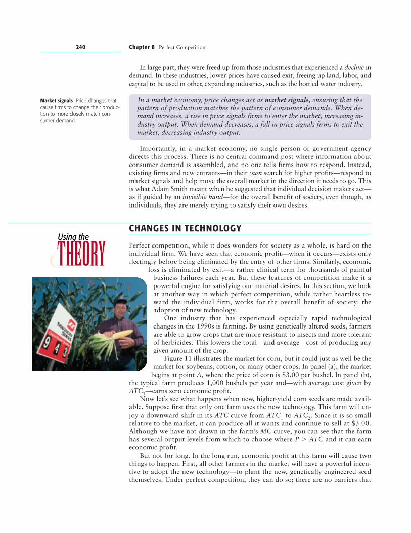
One industry that has experienced especially rapid technologicalchanges in the 1990s is farming. By using genetically altered seeds, farmersare able to grow crops that are more resistant to insects and more tolerantof herbicides. This lowers the total—and average—cost of producing anygiven amount of the crop.

Figure 11 illustrates the market for corn, but it could just as well be themarket for soybeans, cotton, or many other crops. In panel (a), the market

begins at point A, where the price of corn is $3.00 per bushel. In panel (b),the typical farm produces 1,000 bushels per year and—with average cost given byATC1—earns zero economic profit.

Now let’s see what happens when new, higher-yield corn seeds are made avail-able. Suppose first that only one farm uses the new technology. This farm will en-joy a downward shift in its ATC curve from ATC1 to ATC2. Since it is so smallrelative to the market, it can produce all it wants and continue to sell at $3.00.Although we have not drawn in the farm’s MC curve, you can see that the farmhas several output levels from which to choose where P � ATC and it can earneconomic profit.

But not for long. In the long run, economic profit at this farm will cause twothings to happen. First, all other farmers in the market will have a powerful incen-tive to adopt the new technology—to plant the new, genetically engineered seedthemselves. Under perfect competition, they can do so; there are no barriers that


In a market economy, price changes act as market signals, ensuring that thepattern of production matches the pattern of consumer demands. When de-mand increases, a rise in price signals firms to enter the market, increasing in-dustry output. When demand decreases, a fall in price signals firms to exit themarket, decreasing industry output.

Market signals Price changes thatcause firms to change their produc-tion to more closely match con-sumer demand.

THEORYTHEORYUsing the

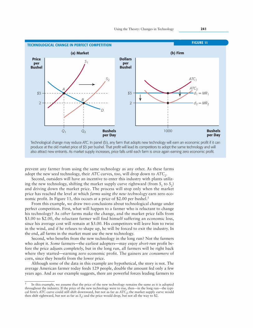
prevent any farmer from using the same technology as any other. As these farmsadopt the new seed technology, their ATC curves, too, will drop down to ATC2.

Second, outsiders will have an incentive to enter this industry with plants utiliz-ing the new technology, shifting the market supply curve rightward (from S1 to S2)and driving down the market price. The process will stop only when the marketprice has reached the level at which farms using the new technology earn zero eco-nomic profit. In Figure 11, this occurs at a price of $2.00 per bushel.5

From this example, we draw two conclusions about technological change underperfect competition. First, what will happen to a farmer who is reluctant to changehis technology? As other farms make the change, and the market price falls from$3.00 to $2.00, the reluctant farmer will find himself suffering an economic loss,since his average cost will remain at $3.00. His competitors will leave him to twistin the wind, and if he refuses to shape up, he will be forced to exit the industry. Inthe end, all farms in the market must use the new technology.

Second, who benefits from the new technology in the long run? Not the farmerswho adopt it. Some farmers—the earliest adopters—may enjoy short-run profit be-fore the price adjusts completely, but in the long run, all farmers will be right backwhere they started—earning zero economic profit. The gainers are consumers ofcorn, since they benefit from the lower price.

Although some of the data in this example are hypothetical, the story is not. Theaverage American farmer today feeds 129 people, double the amount fed only a fewyears ago. And as our example suggests, there are powerful forces leading farmers to

Using the Theory: Changes in Technology 241

5 In this example, we assume that the price of the new technology remains the same as it is adoptedthroughout the industry. If the price of the new technology were to rise, then—in the long run—the typi-cal firm’s ATC curve could still shift downward, but not as far as ATC2; the market supply curve wouldthen shift rightward, but not as far as S2; and the price would drop, but not all the way to $2.

Bushelsper Day

Priceper

Bushel

$3

Q1

S1

2

Q2

A

B

D

S2

(a) Market

1000

ATC1

ATC2d1 = MR1

d2 = MR2

Bushelsper Day

Dollarsper

Bushel

$3

2

(b) Firm

Technological change may reduce ATC. In panel (b), any farm that adopts new technology will earn an economic profit if it canproduce at the old market price of $3 per bushel. That profit will lead its competitors to adopt the same technology and willalso attract new entrants. As market supply increases, price falls until each farm is once again earning zero economic profit.

FIGURE 11TECHNOLOGICAL CHANGE IN PERFECT COMPETITION

adopt new productivity-enhancing technology. Between 1995 and 1999, the fractionof U.S. corn acreage planted with the new seeds increased from zero to about one-half.

More generally, we can summarize the impact of technological change as follows:

Technological advances in many competitive industries—mining, lumber, andfarming, for example—have indeed spread quickly, shifting market supply curvesrapidly and steadily rightward over the past 100 years. Consumers have reaped hugerewards from these advances, but it has not always been easy on individual firms.

This may explain, at least in part, why many small farmers have lobbied forgovernment limits on new agricultural techniques, such as the genetically alteredseeds of our example. Small farmers know they will be the last to obtain these newseeds and so will suffer losses in the short run as other, larger farmers leap ahead ofthem. And in the long run, the most the small farmer can hope for anyway is a re-turn to zero economic profit. Technological change is, indeed, hard on the smallfarmer, but it has also enabled the industry as a whole to feed a growing world pop-ulation at steadily declining prices.


Under perfect competition, a technological advance leads to a rightwardshift of the market supply curve, decreasing market price. In the short run,early adopters may enjoy economic profit, but in the long run, all adopterswill earn zero economic profit. Firms that refuse to use the new technologywill not survive.

Perfect competition is a market structure in which (1) thereare large numbers of buyers and sellers and each buys orsells only a tiny fraction of the total market quantity; (2) sellers offer a standardized product; and (3) sellers caneasily enter or exit from the market. While few real marketssatisfy these conditions precisely, the model is still useful ina wide variety of cases.

Each perfectly competitive firm faces a horizontal de-mand curve; it can sell as much as it wishes at the marketprice. The firm chooses its profit-maximizing output level bysetting marginal cost equal to the market price. Its short-runsupply curve is that part of its MC curve that lies above aver-age variable cost. Total profit is profit per unit (P � ATC)times the profit-maximizing quantity.

In the short run, market price is determined where the mar-ket supply curve—the horizontal sum of all firms’ supplycurves—crosses the market demand curve. In short-run equilib-rium, existing firms can earn a profit (in which case new firmswill enter) or suffer a loss (in which case existing firms willexit). Entry or exit will continue until, in the long run, eachfirm is earning zero economic profit. At each competitive firmin long-run equilibrium, price � marginal cost � minimum av-erage total cost � minimum long-run average total cost.

When demand curves shift, prices change more in theshort run than in the long run. The temporary, exaggeratedprice movements act as market signals, ensuring that outputexpands and contracts in each industry to match the patternof consumer preferences.

S U M M A R Y

market structure perfect competition price taker

shutdown price firm’s supply curve market supply curve

normal profit long-run supply curve increasing cost industry

constant cost industry decreasing cost industry market signals

K E Y T E R M S

1. What are the three characteristics that typify a perfectlycompetitive market? Explain the importance of eachcharacteristic.

2. How do economists justify using the perfectly competi-tive model to analyze markets that clearly do not satisfyone or more of the assumptions of that model?

R E V I E W Q U E S T I O N S

Problems and Exercises 243

3. On a scale of 1 to 5, with 5 being full satisfaction and 1being no satisfaction at all, rank the following markets interms of their satisfaction of the three characteristics ofthe perfectly competitive model. Assign a score for eachcharacteristic and justify your assignment.a. Clothing storesb. Restaurantsc. Book publishingd. Home video game productione. Jet aircraft production

4. Why is the demand curve facing a perfectly competitivefirm infinitely elastic?

5. “To maximize profit, a perfectly competitive firm shouldproduce the level of output at which marginal cost isequal to price.” True, false, or uncertain? Explain.

6. To calculate profit (or loss) for a perfectly competitivefirm, we look at the difference between P and ATC, but todetermine the profit-maximizing (or loss-minimizing) levelof output, we focus on price and marginal cost. Why?

7. Discuss the following statement: “Economists need topay more attention to the real business world. Theirmodel of perfect competition predicts that firms in a mar-ket will end up earning no profit—nothing above costs.As any accountant can tell you, if you look at the balancesheets of most businesses in any industry, their revenueexceeds their costs; they do, in fact, make a profit.”

8. True, false, or uncertain? Explain your answer.a. A perfectly competitive firm is profitable when price

exceeds minimum AVC.b. A competitive firm’s supply curve is just its MC

curve.

9. What is the fundamental characteristic that distinguishesthe short run from the long run in the analysis of a com-petitive market?

10. True or false? In a perfectly competitive market, an in-crease in output requires a high price in the short run,but not in the long run. Justify your answer.

1. In 1999, (1) sales of sport utility vehicles (SUVs) sky-rocketed, and (2) the price of gasoline rose. BecauseSUVs get lower gasoline mileage than the automobilesthey replaced, their owners ended up buying more gaso-line even as the price per gallon rose. Is this a violationof the law of demand?

2. Suppose that a perfectly competitive firm has the follow-ing total variable costs (TVC):

Quantity: 0 1 2 3 4 5 6TVC: 0 6 11 15 18 22 28

It also has fixed costs of $6. If the market price is $5per unit:a. Find the firm’s profit-maximizing quantity using the

marginal revenue and marginal cost approach.b. Check your results by re-solving the problem using the

total revenue and total cost approach. Is the firm earn-ing a positive profit, suffering a loss, or breaking even?

3. Assume that the market for cardboard is perfectly com-petitive (if not very exciting). In each of the followingscenarios, should a typical firm continue to produce orshould it shut down in the short run? Draw a diagramthat illustrates the firm’s situation in each case.a. Minimum ATC � $2.00

Minimum AVC � $1.50Market price � $1.75

b. MR � $1.00Minimum AVC � $1.50Minimum ATC � $2.00

4. The following table gives quantity supplied and quantitydemanded at various prices in the perfectly competitivemeat packing market:

QS QDPrice (per lb.) (in millions of lbs.)

$1.00 10 100$1.25 15 90$1.50 25 75$1.75 40 63$2.00 55 55$2.25 65 40

Assume that each firm in the meat-packing industry facesthe following cost structure:

Pounds TC

60,000 $110,00061,000 $111,00062,000 $112,00063,000 $115,000

a. What is the profit-maximizing output level for thetypical firm? (Hint: Calculate MC for each change in

P R O B L E M S A N D E X E R C I S E S

output, then find the equilibrium price, and calculateMR for each change in output.)

b. Is this market in long-run equilibrium? Why or whynot? (Hint: Calculate ATC.)

c. What do you expect to happen to the number ofmeat-packing firms over the long run? Why?

5. Assume that the kitty litter industry is perfectly competi-tive and is presently in long-run equilibrium:a. Draw diagrams for both the market and a typical

firm, showing equilibrium price and quantity for themarket, and MC, ATC, AVC, MR, and the demandcurve for the firm.

b. Your friend has always had a passion to get into thekitty litter business. If the market is in long-run equi-librium, will it be profitable for him to jump in head-first (so to speak)? Why or why not?

c. Suppose people begin to prefer dogs as pets, and catownership declines. Show on your diagrams frompart (a) what happens in the industry and the firm inthe long run.

d. Is the market supply curve flatter in the short or inthe long run? Why?

6. In a perfect competitive, increasing cost industry, is thelong-run supply curve always flatter than the short-runmarket supply curve? Explain.

7. With a 4-panel diagram similar to Figure 10, show whathappens in an increasing-cost industry when the marketdemand curve shifts leftward.


1. Figure 10 in the chapter shows the long-run adjustmentprocess after an increase in demand. The figure assumesthat input prices rise as industry output expands. However,in some industries, input prices might fall as output ex-pands. This would occur if firms that produce inputs enjoyeconomies of scale (see Chapter 6). In this case, an increasein the production of inputs would actually lower their costper unit, and ultimately lower the price of inputs.a. Redraw Figure 10 under the assumption that input

prices fall as industry output expands. Illustrate whathappens in the short run and in the long run after themarket demand curve shifts rightward.

b. Trace out the long-run supply curve for this industry.How does it differ from the long-run supply curve inFigure 10?

c. How might your new figure help explain why theprices of personal computers have fallen steadily overthe past two decades?

2. In rare cases, existing technologies are found to be pol-luting or physically dangerous, and are banned. Reviewthe “Using the Theory” section of this chapter. Then,show graphically the effects of banning a technologythat is in common use in a competitive industry. (Hint:After the technology is banned, what will happen to theaverage cost curve?)

C H A L L E N G E Q U E S T I O N S

2. Rent the movie Trading Places, starring Eddie Murphyand Dan Ackroyd. Enjoy the movie, but pay special at-tention to the scene near the end where Billy Ray andLouis participate in an auction of orange juice futures.How does the arrival of new information affect the priceof futures contracts? Try to model the situation usingsupply-and-demand curves.

E X P E R I E N T I A L E X E R C I S E S

1. Economics America has an interestingmodule on the economics of Internet ac-cess (http://www.economicsamerica.org/econedlink/newsline/internet/index.html).Is provision of Internet access a competitive industry?How would you use supply-and-demand tools tomodel recent developments in Internet pricing?

http://

Documents

PERFECT COMPETITION - virtualpanic.comvirtualpanic.com/anonymousftplistings/ebooks/ECONOMICS/8 - Perfect...ers and sellers come together, ... may think of an intense, personal rivalry,