1

Performing Raster Operations using ArcGIS Spatial Analyst

Prepared by

Venkatesh Merwade

School of Civil Engineering, Purdue University

vmerwade@purdue.edu

August 2012

1.0 Purpose

The purpose of this exercise is to explore some of the functionalities of the ArcGIS

Spatial Analyst extension.

2.0 Computer and Data Requirements

To complete this exercise, you will need ArcGIS 10 with Spatial Analyst Extension. Data

for this exercise is available at ftp://ftp.ecn.purdue.edu/vmerwade/class/ce549/ in

Lab08_20 folder.

3.0 Exploring a DEM

Things that we need to know about a DEM are its projections, cell size, type (integer or

float), format, number of bands and size. These can be found by right-clicking on the

DEM and then selecting Properties. Within the Properties window, select the Source tab,

and you will get all the information that you need about the dataset. However, if the DEM

is in geographic coordinates, the cell size will be in decimal degrees which will make no

sense to most people. Similarly processing such a raster (with geographic coordinates) for

hydrologic applications will yield attributes such as river length and flow accumulation

area in units that are non conventional to many hydrologists. Therefore, the first step is to

project a raster in appropriate coordinate system.

4.0 DEM Projection

Any datasets in ArcMap is projected by using ArcGIS Toolbox. If the toolbox is not

already added to your map document, click on the red toolbox button in ArcMap

toolbar to open the toolbox in ArcMap. As you seen in the raster properties, the

geographic projection is already defined for this dataset. In the ArcToolbox, Select Data

Management ToolsProjections and TransformationsRasterProject Raster. (Note:

If there is no projection defined for the raster, the first step is to first define the projection

by selecting the Define Projection toolbar, and then project it using Project Raster tool).

In the project raster window, select your input raster and name the projected output raster

as cedar_proj. Unless you want your output as image (.img) or TIFF (.tiff), do not

provide any extension to the output raster. This will create the output in default GRID

format. Define the coordinate system by pressing the spatial reference properties button

2

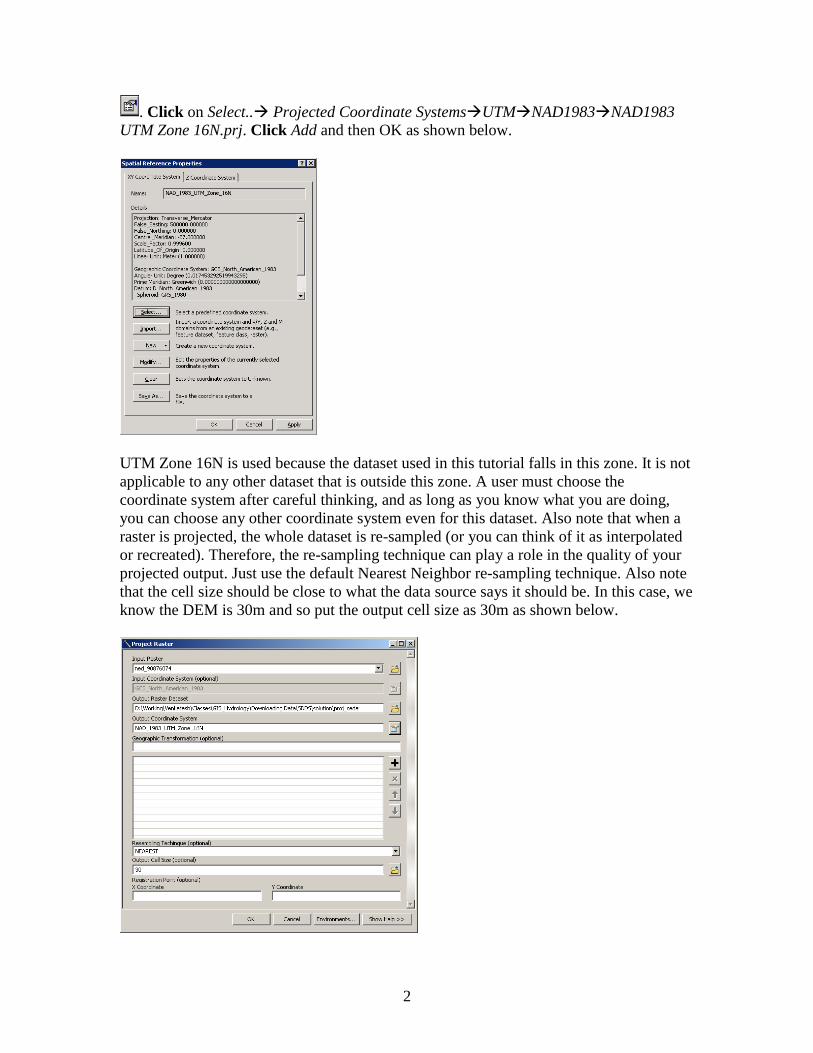
. Click on Select.. Projected Coordinate SystemsUTMNAD1983NAD1983

UTM Zone 16N.prj. Click Add and then OK as shown below.

UTM Zone 16N is used because the dataset used in this tutorial falls in this zone. It is not

applicable to any other dataset that is outside this zone. A user must choose the

coordinate system after careful thinking, and as long as you know what you are doing,

you can choose any other coordinate system even for this dataset. Also note that when a

raster is projected, the whole dataset is re-sampled (or you can think of it as interpolated

or recreated). Therefore, the re-sampling technique can play a role in the quality of your

projected output. Just use the default Nearest Neighbor re-sampling technique. Also note

that the cell size should be close to what the data source says it should be. In this case, we

know the DEM is 30m and so put the output cell size as 30m as shown below.

3

Click OK. The new projected raster (cedar_proj) will be added to the map document

after the process is complete. Change the coordinates system of the Data Frame to see

the data in projected coordinates. Now lets see what we can do with this DEM by using

Spatial Analyst Extension in ArcMap. If you have purchased Spatial Analyst extension

(which is the case for Purdue University), then you should be able to load the extension

by selecting CustomizeExtensionsSpatial Analyst.

5.0 Clipping a DEM

Most often (or always), we need to “clip” a raster to a study area that is smaller than the

entire domain of the raster dataset. A smaller dataset in turn reduces processing time, thus

increasing efficiency. In order to clip a raster, you should have the boundary of your

study area. There are several ways of clipping a raster to a polygon mask. In this exercise

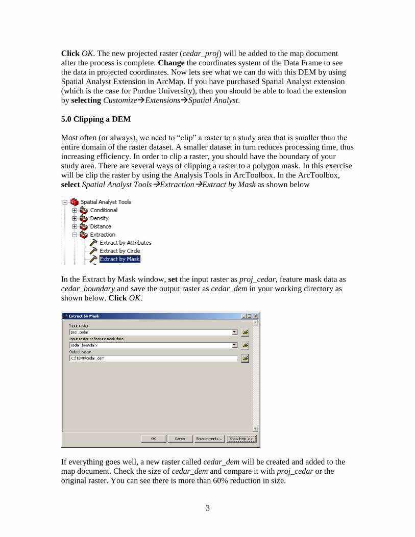
will be clip the raster by using the Analysis Tools in ArcToolbox. In the ArcToolbox,

select Spatial Analyst ToolsExtractionExtract by Mask as shown below

In the Extract by Mask window, set the input raster as proj_cedar, feature mask data as

cedar_boundary and save the output raster as cedar_dem in your working directory as

shown below. Click OK.

If everything goes well, a new raster called cedar_dem will be created and added to the

map document. Check the size of cedar_dem and compare it with proj_cedar or the

original raster. You can see there is more than 60% reduction in size.

4

6.0 Raster Conversion from Float to Integer

Another way of reducing the size of a DEM is by converting it to an integer type. In

addition, some of the spatial analyst tools (such as converting raster to features) work

only with integer type rasters. Therefore, having an integer raster is desirable under

certain circumstances. A float type raster can be converted to an integer type by using the

Int function in raster calculator, but this will chop off all the decimals compromising the

quality of the dataset. This issue, however, can be resolved by using other functions in

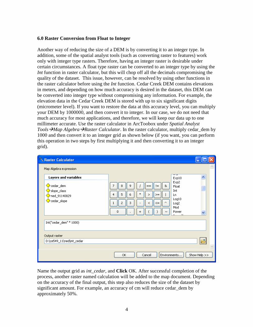
the raster calculator before using the Int function. Cedar Creek DEM contains elevations

in meters, and depending on how much accuracy is desired in the dataset, this DEM can

be converted into integer type without compromising any information. For example, the

elevation data in the Cedar Creek DEM is stored with up to six significant digits

(micrometer level). If you want to restore the data at this accuracy level, you can multiply

your DEM by 1000000, and then convert it to integer. In our case, we do not need that

much accuracy for most applications, and therefore, we will keep our data up to one

millimeter accurate. Use the raster calculator in ArcToobox under Spatial Analyst

ToolsMap AlgebraRaster Calculator. In the raster calculator, multiply cedar_dem by

1000 and then convert it to an integer grid as shown below (if you want, you can perform

this operation in two steps by first multiplying it and then converting it to an integer

grid).

Name the output grid as int_cedar, and Click OK. After successful completion of the

process, another raster named calculation will be added to the map document. Depending

on the accuracy of the final output, this step also reduces the size of the dataset by

significant amount. For example, an accuracy of cm will reduce cedar_dem by

approximately 50%.

5

Most operations in Raster Calculator are self-explanatory, and you should be able to use

them without any problem.

7.0 Calculating Slope

There are two options for computing slope grid in Spatial Analyst from elevation data.

These include slope in percent and in degrees. The slope function in Spatial Analyst

calculates the maximum rate of change in value from that cell to its neighbors (steepest

downhill descent from the cell). ArcMap uses the following algorithm to compute the

slope in degrees:

slope_degrees = ATAN ( √ ( [dz/dx]2 + [dz/dy]

2 ) ) * 57.29578

where [dz/dx] = ((c + 2f + i) - (a + 2d + g) / (8 * cell size) in the figure below and [dz/dy]

= ((g + 2h + i) - (a + 2b + c)) / (8 * cell_size)

Slope in percent is then the tangent of the angle obtained by converting slope_degrees to

radians ( = slope_degree* /180) times 100. So a 45 degree slope will give a 100% slope

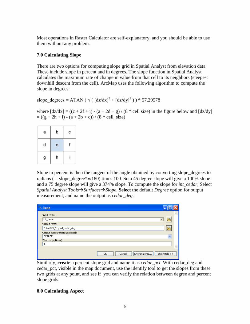
and a 75 degree slope will give a 374% slope. To compute the slope for int_cedar, Select

Spatial Analyst ToolsSurfacesSlope. Select the default Degree option for output

measurement, and name the output as cedar_deg.

Similarly, create a percent slope grid and name it as cedar_pct. With cedar_deg and

cedar_pct, visible in the map document, use the identify tool to get the slopes from these

two grids at any point, and see if you can verify the relation between degree and percent

slope grids.

8.0 Calculating Aspect

6

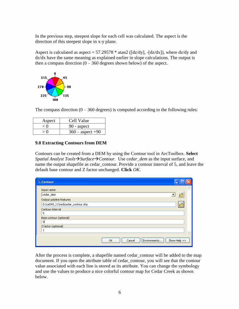
In the previous step, steepest slope for each cell was calculated. The aspect is the

direction of this steepest slope in x-y plane.

Aspect is calculated as aspect = 57.29578 * atan2 ([dz/dy], -[dz/dx]), where dz/dy and

dz/dx have the same meaning as explained earlier in slope calculations. The output is

then a compass direction (0 – 360 degrees shown below) of the aspect.

The compass direction (0 – 360 degrees) is computed according to the following rules:

Aspect Cell Value

< 0 90 - aspect

> 0 360 – aspect +90

9.0 Extracting Contours from DEM

Contours can be created from a DEM by using the Contour tool in ArcToolbox. Select

Spatial Analyst ToolsSurfaceContour. Use cedar_dem as the input surface, and

name the output shapefile as cedar_contour. Provide a contour interval of 5, and leave the

default base contour and Z factor unchanged. Click OK.

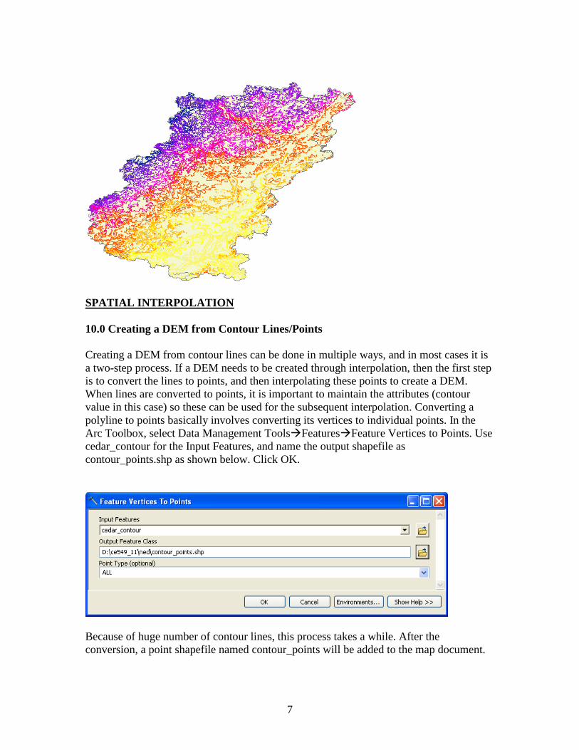
After the process is complete, a shapefile named cedar_contour will be added to the map

document. If you open the attribute table of cedar_contour, you will see that the contour

value associated with each line is stored as its attribute. You can change the symbology

and use the values to produce a nice colorful contour map for Cedar Creek as shown

below.

7

SPATIAL INTERPOLATION

10.0 Creating a DEM from Contour Lines/Points

Creating a DEM from contour lines can be done in multiple ways, and in most cases it is

a two-step process. If a DEM needs to be created through interpolation, then the first step

is to convert the lines to points, and then interpolating these points to create a DEM.

When lines are converted to points, it is important to maintain the attributes (contour

value in this case) so these can be used for the subsequent interpolation. Converting a

polyline to points basically involves converting its vertices to individual points. In the

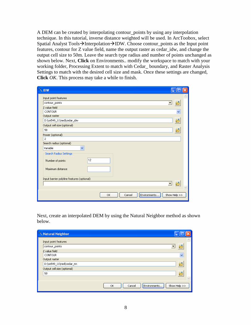
Arc Toolbox, select Data Management ToolsFeaturesFeature Vertices to Points. Use

cedar_contour for the Input Features, and name the output shapefile as

contour_points.shp as shown below. Click OK.

Because of huge number of contour lines, this process takes a while. After the

conversion, a point shapefile named contour_points will be added to the map document.

8

A DEM can be created by interpolating contour_points by using any interpolation

technique. In this tutorial, inverse distance weighted will be used. In ArcToobox, select

Spatial Analyst ToolsInterpolationIDW. Choose contour_points as the Input point

features, contour for Z value field, name the output raster as cedar_idw, and change the

output cell size to 50m. Leave the search type radius and number of points unchanged as

shown below. Next, Click on Environments.. modify the workspace to match with your

working folder, Processing Extent to match with Cedar_ boundary, and Raster Analysis

Settings to match with the desired cell size and mask. Once these settings are changed,

Click OK. This process may take a while to finish.

Next, create an interpolated DEM by using the Natural Neighbor method as shown

below.

9

Using the contour_points as input, contour attribute for z field, and a cell size of 50m,

Again, change the analysis settings by selecting the Environments.. button, and then click

OK. A new raster cedar_nn will be added to the map document.

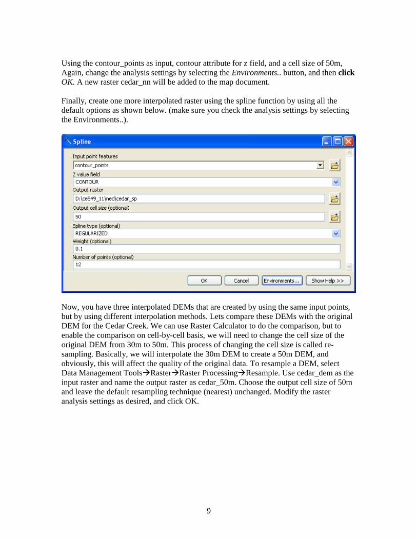
Finally, create one more interpolated raster using the spline function by using all the

default options as shown below. (make sure you check the analysis settings by selecting

the Environments..).

Now, you have three interpolated DEMs that are created by using the same input points,

but by using different interpolation methods. Lets compare these DEMs with the original

DEM for the Cedar Creek. We can use Raster Calculator to do the comparison, but to

enable the comparison on cell-by-cell basis, we will need to change the cell size of the

original DEM from 30m to 50m. This process of changing the cell size is called re-

sampling. Basically, we will interpolate the 30m DEM to create a 50m DEM, and

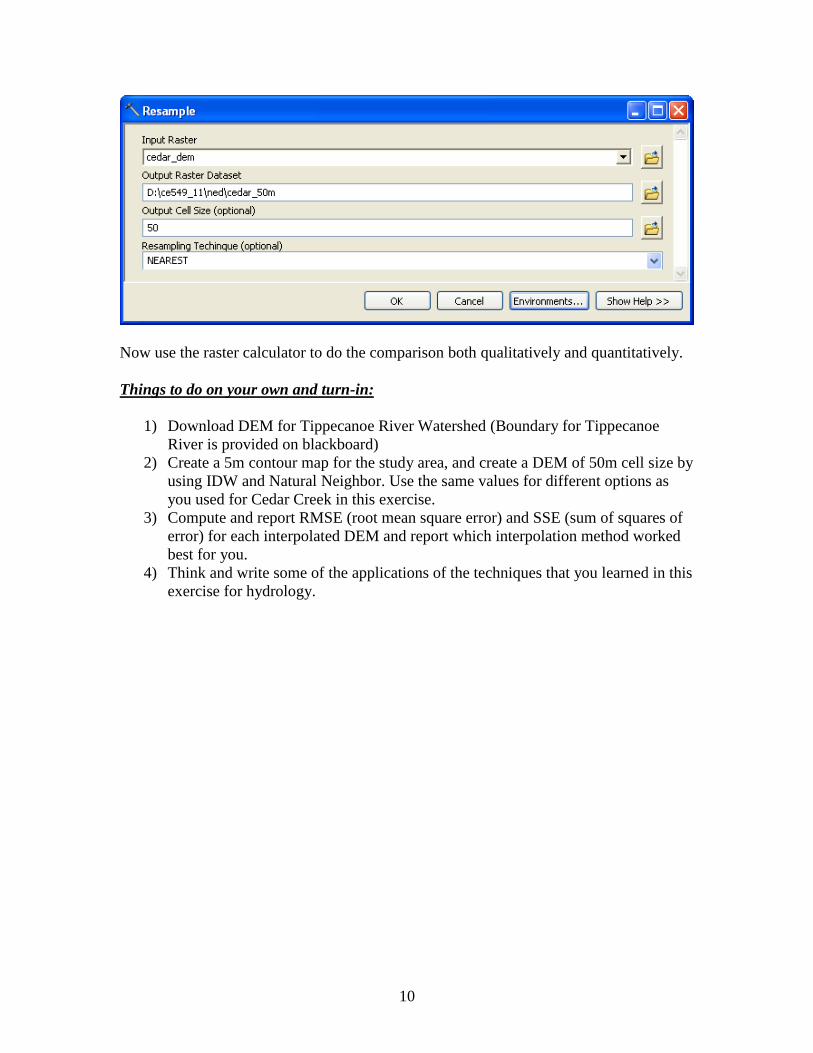
obviously, this will affect the quality of the original data. To resample a DEM, select

Data Management ToolsRasterRaster ProcessingResample. Use cedar_dem as the

input raster and name the output raster as cedar_50m. Choose the output cell size of 50m

and leave the default resampling technique (nearest) unchanged. Modify the raster

analysis settings as desired, and click OK.

10

Now use the raster calculator to do the comparison both qualitatively and quantitatively.

Things to do on your own and turn-in:

1) Download DEM for Tippecanoe River Watershed (Boundary for Tippecanoe

River is provided on blackboard)

2) Create a 5m contour map for the study area, and create a DEM of 50m cell size by

using IDW and Natural Neighbor. Use the same values for different options as

you used for Cedar Creek in this exercise.

3) Compute and report RMSE (root mean square error) and SSE (sum of squares of

error) for each interpolated DEM and report which interpolation method worked

best for you.

4) Think and write some of the applications of the techniques that you learned in this

exercise for hydrology.