Persuasion and empathy in salesperson-customerinteractions

Julio J. Rotemberg∗

August 4, 2010

Abstract

I consider a setting where firms can ask their salespeople to spend time and effortpersuading customers. The equilibrium often features heterogeneity, with some sales-people being asked to persuade customers while others are not. Persuasive messagescan either increase or decrease welfare, with price and quantity data generally beinginsufficient to determine whether welfare rises or falls. If one supposes that salespeo-ple with different levels of empathy sort themselves across different selling job, thecross-sectional correlation between a salesperson’s sales and his or her empathy, can behelpful in determining whether persuasion is good or bad for consumers. JEL: M31,D64, D83

∗Harvard Business School, Soldiers Field, Boston, MA 02163, jrotemberg@hbs.edu. I wish to thankseminar participants at Boston University for helpful comments.

Out of 145 million civilian employees in 2008, the U.S. Bureau of Labor Statistics classi-

fied 16 million as working in “Sales and Related Occupations”.1 While there is a great deal

of variety in what these individuals do, an important role of many of them is to persuade

potential customers to buy the goods and services offered by their employers.2 The methods

used by salespeople to do so are shaped, at least to some extent, by their employers. One

standard approach for influencing salespeople is to pair new salespeople with more experi-

enced ones, so that the latter can teach the former. It is also common for more experienced

salespeople to be accompanied occasionally on sales calls by managers who monitor their

behavior.3 Some companies also provide their salespeople with written instruction on how

they are supposed to conduct themselves with customers.4

This paper considers three issues. The first is the nature of the equilibrium when firms

have the option of asking their employees to spend time and effort influencing their customers’

willingness to pay for their product. The second is whether the persuasive techniques adopted

in equilibrium increase or reduce welfare. In common with Becker and Murphy’s (1993)

analysis of persuasive advertising, techniques that have the same effect on profits, prices

and quantities sold may have quite different effects on consumer welfare. Inducing firms to

modify the content of their persuasive sales pitches thus has the potential to increase overall

welfare. Lastly, the paper studies how potential employees with different degrees of empathy

for their customers sort themselves across the sales jobs within a particular industry. The

resulting correlation between a salesperson’s empathy and his or her level of sales can then

help determine whether the persuasion methods used in an industry are good or bad for

consumers.

Consistent with the idea that the persuasion techniques used by salespeople sometimes

1By comparison, only 6.1% were classified as salesworkers in 1968 so that this activity shows no sign ofwaning.

2Some workers in this occupational group, particularly cashiers, have little time for this activity. Therewere only about 3 million workers classified as cashiers in 2008, however.

3See Stroh (1978, p. 299–300). Stroh (1978, p. 303) goes on to say “The observing supervisor will notethe amount of aggression and judge its degree of being appropriate.”

4See Friedman (2004, p. 124–128) for a discussion of John Patterson’s introduction of such scripts atNCR.

1

increase welfare while other times they reduce it, the empirical literature studying cross-

sectional correlations between salesperson empathy and salesperson effectiveness has pro-

duced mixed results. The early study of Tobolski and Kerr (1952) found a positive relation-

ship between a measure of dispositional empathy and the effectiveness of new car salesmen

at two dealers. By contrast, negative correlations with various measures of effectiveness are

reported by Lamont and Lundstrom (1977) for a sample of building supply salesmen. Lastly,

Dawson et al. (1992) reports a very weak relationship between empathy and sales.5

One way of thinking about the extensive literature focused on consumer search is that

it considers random encounters between consumers and salespeople, where the only role of

salespeople is to give a price quote. This paper maintains the framework of random encoun-

ters but lets salespeople carry out effort to change the amount of utility that their customers

obtain from either purchasing or not purchasing the good. The model I consider is a modified

version of Burdett and Judd (1983) so that some consumers encounter a single salesperson

while the rest encounters two. As a result, the equilibrium features price dispersion and firms

that charge lower prices sell more. Empathetic salespeople prefer jobs where they increase

the happiness of their consumers, and thus prefer jobs with lower prices. This implies that,

in the baseline model, empathetic salespeople will seek jobs with low prices and high sales;

and this tends to create a positive correlation between empathy and sales.

When this model is modified so that salespeople can expend effort to persuade consumers,

this correlation comes to depend both on the likelihood that a salesperson can persuade a

consumer and on whether the salesperson increases the value of buying or increases the cost

of not buying. The former enhances welfare while the latter reduces it. In the case every

customer is persuaded by any salesperson expending the necessary effort, the correlation

5More recent regression studies seeking to explain the performance of salespeople have tended to focuson “customer orientation,” (CO) measured as in Saxe and Weitz (1982) rather than on empathy per se. Thetwo variables are strongly correlated with one another (see Widmier (2002) and Stock and Hoyer (2005))and closely related conceptually. The CO scale gives considerable weight to agreement with the statements“I try to achieve my goals by satisfying customers,” and “A good salesperson has to have the customer’sbest interest in mind.” Both of these fit well with the way I model empathy, which is by supposing thatthe salesperson’s objective includes the utility of his customers. The meta-analysis of Franke and Park(2006) shows that the correlation between salespeople’s self-reported customer orientation and the level ofperformance as evaluated by their managers is quite weak.

2

between empathy and sales can be negative, but only if persuasion reduces welfare. The

reason for this is that, in this case, sales are enhanced by techniques that are costly to

consumers, and empathetic salespeople want to avoid hurting their customers.

While the methods for increasing sales that I consider are abstract, they fit with some

of the suggestions from the qualitative literature on “non-informative” selling techniques.

One widespread suggestion is that salespeople should devote effort at being liked by their

potential customers (prospects). Girad (1989, p. 17) says “The prospect must like you.”

Baber (1997, p. 40) says ”Customers like to do business with people and companies they

like.” Baber (1997) goes on to suggest that customers will “like you” if ”they feel comfortable

with you (you are like them naturally, through mirroring, or otherwise).” The technique of

“mirroring,” which Baber (1997, p. 39) describes and recommends, involves imitating the

speech cadence and the body posture of prospects. The ethnographic analysis of Bone (2006,

p. 61) shows that imitation was common among the “accomplished sellers” of the company

he studied.

Perceived similarity has been shown to have two related consequences in the social psy-

chology literature. First, Byrne (1961) shows that subjects who believe that a stranger

shares more of their attitudes report more “liking” for this stranger, and several papers have

shown this finding to be robust. Consistent with this increased liking, a second group of

papers has shown that perceived similarity leads to more helping.6 A simple interpretation of

these findings is that that people feel more empathy towards (or more altruism) for people

that they perceive as being more similar to themselves.7 In a sales context, creating the

impression that the salesperson is similar to the prospect may thus enhance the customer’s

altruism towards the salesperson.

This induced altruism can both raise the value that a consumer attaches to a purchase

6See, for example, Suedfeld et al. (1972) and Gueguen et al (2005). Substantively, these findings areclosely related to those of studies based on the “lost letter technique” of Milgram et al. (1965). Thesestudies show that people are more likely to fulfill the desires of people whose unmailed letters they find onthe ground if they agree with the attitudes of the senders of these letters. See, particularly, Tucker et al.(1977).

7See Rotemberg (2009) for an application to the domain of voting.

3

and increase his cost from not purchasing.8 Consumers rationally expect salespeople to be

more pleased when they complete a sale than when they do not. As a result, the act of

purchasing can give consumers some vicarious pleasure. It can also lead consumers to suffer

some vicarious losses when they fail to purchase. Arguably, these vicarious losses can be

increased if the salesperson convinces the consumer that he already expected the sale to be

completed, because this can lead the consumer to feel more guilt or vicarious disappointment

if he does not buy.9

This fits with NCR’s 1887 advice to its salespeople that they should “not ask for an order

[but] take for granted that he will buy. Say to him ‘Now, Mr. Blank, what color shall I

make it?’ or ‘How soon do you want delivery?’ ”10 Girard (1989, p. 44) and MDRT (1999,

p. 26) give a number of contemporary examples of this approach. As MDRT (1999) states,

the idea behind this technique for “closing’ sales is to make it difficult for the prospect to

avoid purchasing the good.

The company described in Bone (2006) used an additional technique to raise the cost of

not buying. Salespeople at this company were expected to obtain agreement from their cus-

tomers about desirable aspects of the product before they offered a price quote. If customers

did not agree to buy, salespeople would ask for their reasons. Salespeople would then subtly

suggest that the customer was being “disingenuous” or “irrational” if he tried to wiggle out

by backtracking on some of his earlier statements.

Since these techniques are unpleasant for would-be buyers, they would not appeal to

salespeople whose utility depends positively on the utility of their customers. This should

lead salespeople with relatively high levels of altruism (or empathy) for their customers

to self-select out of jobs that require these techniques. The logic is the same as that in

8This is broadly consistent with Calvo-Armengol and Jackson (2010) who model peers as able to exert“positive pressure,” where they lower a peer’s cost of taking an action and “negative pressure,” where theyincrease the cost of not taking the action in question.

9A rare, but nonetheless effective method to obtain a sale by evoking sympathy is reported in Bone (2006,p. 90). He depicts a salesperson who, when customers declared an intention not to buy, routinely “burst intotears” while saying that she was “in trouble with the boss.” This sales method led at least some customersto buy.

10See Friedman (2004, p. 126)

4

Prendergast (2007), who considers the job choices of bureaucrats that vary in their concern

for their clients.

One difference between the Prendergast (2007) model and the current one is that I

am focusing on aspects of employee behavior that can be monitored. The result is that,

under some additional conditions that I impose, employers are indifferent with respect to

the altruism of their employees. Employees should thus be willing to reveal their empathy

truthfully. This still leaves the question of whether the questionnaires that are typically

employed to measure empathy do so reliably. Some evidence for this is reported in Singer et

al. (2004).

Like the earlier study of Hutchison et al. (1999), Singer et al. (2004) show that pain

related neurons are activated not only in response to painful stimuli to the self but also in

response to painful stimuli that are applied to others in the subject’s presence. These neu-

rological measurements of empathy fit into a literature in which neurons of an individual are

observed to “mirror” the behavior of another person’s neurons. Perhaps the most remarkable

finding in Singer et al. (2004) is that the size of the “mirror neuron” responses they record is

larger in subjects who score higher on the Balanced Emotional Empathy Scale of Mehrabian

and Epstein (1972). The same is true for subjects who score higher in the Empathic Concern

Scale of Davis (1980). These scales are based on answers to self-administered questionnaires.

The paper proceeds as follows. Section 2 introduces the model of costly persuasive effort.

As in most of the paper, this effort is assumed to affect the willingness to pay of all customers

by the same amount. If this effort costs sufficiently little, all salespeople engage in it, while

none do so if it is sufficiently costly. More interestingly, there is a range of costs for this

effort so that some salespeople actively “sell” their products while others do not. The ones

that do tend to charge higher prices to recover their additional selling costs. They also sell

their product more frequently.

Section 2 also shows that, using only data on prices and quantities, selling activities that

increase the attractiveness of the product to consumers are indistinguishable from selling

activities that reduce the desirability of not buying from a particular salesperson. Section

5

3 then shows that the welfare effect of these two kinds of selling efforts are quite different.

The logic is quite similar to that in Becker and Murphy (1993), though there are some

differences between the effects of persuasive advertising and persuasive selling that I note.

Section 4 discusses employee preferences to prepare the ground for the sorting analysis of

Section 5. Section 6 considers an extension where the effectiveness of the selling effort is

stochastic because a fraction of customers is immune to the persuasive efforts of salespeople.

This brings the model closer to Eliaz and Spiegler (2006), Gabaix and Laibson (2006) and

Armstrong and Chen (2008), who consider models where consumers differ in their naivete.

Section 6 shows that the presence of consumers who are susceptible to persuasive efforts by

salespeople tends to make those that are immune worse off, which is reminiscent of Armstrong

and Chen’s (2008) finding that the existence of naive consumers can reduce the welfare of

sophisticated ones. Section 7 contains some concluding remarks.

1 A deterministic model of persuasive selling

A large number N of firms sell a good that they can procure at marginal cost m. Each one

does so through a single salesperson.11 Each salesperson, in turn, is visited by µ prospects

whose initial valuation for a single unit of the good equals v, and who have no use for

additional units. The µ potential customers of each salesperson are drawn independently

from the population of consumers. As in Burdett and Judd (1983), a fraction θ of all

consumers visits just one salesperson, while the rest visit two.

Salespeople can expend extra effort and thereby increase their customers’ willingness to

pay. As discussed in the introduction, they can do so by either increasing the utility of

purchasing or by reducing the utility from failing to purchase. I thus suppose that, after a

prospect interacts with salesperson i, he assigns a value of v + gi to obtaining the good from

i while he suffers a loss `i if he does not buy it from i. This implies that a consumer prefers

11The assumption that each firm has a single salesperson is made for simplicity of exposition. The modelcan equally well be interpreted as one where each firm has many salespeople, each of which is assigned apre-specified job.

6

buying from i than not buying at all if

v + gi − pi ≥ −`i or v + ki ≥ pi where ki ≡ gi + `i. (1)

If the prospect visits only i, this condition induces him to purchase the good. If he visits

two sellers i and j, he buys from i if, in addition,

v + gi − pi − `j > v + gj − pj − `i or v + ki − pi > v + kj − pj. (2)

If (1) is true and (2) holds as an equality, the consumer is equally willing to buy from

either salesperson and I suppose he chooses i with probability 1/2. If the inequality in (2) is

reversed and (1) holds for j, the consumer buys from j. It follows that, from the perspective

of a consumer’s purchase decision, gi and `i matter only through their sum ki. As I discuss

below, consumer welfare also depends on the individual components g and `. However, the

derivation of an equilibrium is simplified by focusing solely on ki. To simplify further, I

suppose that there is exists only one strictly positive level of effort, and that this leads ki to

equals the constant k. If, instead, the salesperson makes no effort, ki = 0.

Each firm sets a single price and effort level, and these apply to every interaction of its

salesperson.12 Firms set prices and salesperson effort to maximize profits. If firm i wishes its

salesperson to set ki = k, it has to compensate him an extra we for each customer contact.

For the moment, the level of this extra compensation, as well as the base wage w are taken

as fixed.

While the number of firms is finite, they are treated as sufficiently numerous that the

distribution of prices across firms can be well approximated by a continuous density. An

equilibrium is then a distribution of prices such that no firm has an incentive to deviate

because they earn the same profits at all the prices that are charged by a positive density of

firms and would earn lower profits if they charged any other price. Assuming that µθ(v−m) >

w, as I do throughout, the equilibrium satisfies

12This assumption is inessential at this point. Since a range of prices gives the same profits in equilibrium,nothing would be lost by letting salespeople use different prices (and possibly different effort levels) indifferent sales encounters. This is no longer true below when I let salespeople differ in their attitudestowards customers.

7

Proposition 1. a)(Burdett and Judd 1983) If k < we, all firms set ki = 0 and the equilibrium

price has support {θv + (1− θ)m, v} with cumulative density function

Fn(p) = 1− θ(v − p)

(1− θ)(p−m). (3)

b) If we < θk, all firms set ki = k and each firm earns expected profits of µ[θ(v + k −m)− we]− w. The equilibrium price distribution across firms has support {θ(v + k) + (1−θ)m, (v + k)} with cdf

Fa(p) = 1− θ(v + k − p)

(1− θ)(p−m). (4)

c) If θk ≤ we ≤ k, a fraction γ = (1− we/k)/(1− θ) of firms require their employees to

set ki = k for each customer contact while the rest require ki = 0. All firms have expected

profits of µθ(v −m) − w. The firms with ki = 0 have a distribution of prices with support

{p∗, v} where

p∗ = m + (v −m)θk/we,

and a cdf of prices given by

F0(p) = 1− θ(v − p)

(we/k − θ)(p−m). (5)

The firms with ki = k have a distribution of prices with support {p−, p∗ + k} where

p− = we + θv + (1− θ)m.

The cdf of their prices given by

Fk(p) =p− p−

(1− we/k)(p−m). (6)

For a given ki, the main qualitative conclusion of this proposition is the same as that

of Burdett and Judd (1983). This is that prices are dispersed in equilibrium with all firms

making the same expected profits because those that post higher prices sell with lower

frequency. While this correlation between price and quantity is important for what follows,

the main novelty in the proposition lies in its conclusions regarding the extent to which firms

use salespeople to persuade customers to buy.

8

The case where k < we is the one covered by Burdett and Judd (1983) and can be

interpreted as one where firms do not have access to any method for persuading customers.

Thus, going from a situations with k < we to one where we < k can be thought of as

involving the discovery of a sales method, an increase in the susceptibility of customers to

a sales method or the elimination of a law that bans a particular method. Keeping these

interpretations in mind, I now discuss how the nature of equilibria change as we varies relative

to k.

The relatively radical change from the case where we > k to the case where we < θk

leads every firm to adopt the persuasion method in question. This is the easiest change to

analyze because the distribution of prices that applies in the former case (3) is the same as

the one that applies in the latter case (4) if v is substituted by v + k. Thus, (4) can be used

to analyze the effect on price of an innovation that is always implemented and raises the

customer’s willingness to pay by k. Rewriting this equation slightly, we have

p =θ(v + k −m) + m

1− (1− θ)Fa(p).

This says that a one dollar increase in k raises the highest price (the one for which Fa(p) = 1)

by one dollar. However, the prices such that Fa(p) = x < 1 rise by only θ/(1 − (1 − θ)x)

dollars, which is less than one dollar. This suggests that consumers’ whose valuation rises

by k are better off as a result of this innovation, while consumers whose valuation for the

good does not rise are worse off. A formal proof of this is provided below.

The intermediate case where θk < we < k is the most interesting one, because it leads

to heterogeneity both in prices and in the tactics used by salespeople. It also leads to two

different distributions of prices depending on the value of ki. The highest price charged by

a firm with ki = k exceeds (by k) the lowest price charged by firms with k = 0. If the lowest

price charged by firms with ki = k (which equals [m + we + θ(v −m)]) exceeds v, the two

distributions do not overlap. This requires that we > (1 − θ)(v − m), which is satisfied if

either few customers have access to two offers or if the cost of raising the valuation by k

is substantial relative to the gap between consumer value and marginal cost. As a result,

9

outcomes without overlap in the two price distributions may be relatively rare. Still, this

case is conceptually interesting because it shows that this extension of Burdett and Judd

(1983) makes it possible for the overall price distribution to have a hole, something that is

not possible in the standard case where there is no effort by salespeople.

I now turn to an analysis of the expected quantities sold by different salespeople. Let qi

denote the probability that the salesperson working for firm i makes a sale to a customer,

so that this salesperson’s expected sales equal µqi. An important corollary of Proposition 1

is that salespeople who work for firms that set ki = k have larger expected sales than those

that work for firms that set ki = 0. In particular

Proposition 2. If, for two firms i and j, ki = k and kj = 0, qi ≥ we/k ≥ qj. The second

inequality is strict unless the price of firm j equals p∗ while the first inequality is strict unless

the price of firm i equals p∗ + k.

The intuitive logic of this proposition is that firms are more willing to incur the cost we

if they are relatively likely to recover this cost through additional sales. Put differently, a

firm that would have charged a low price and sold relatively frequently if the technology for

raising k was unavailable has more to gain by setting ki = k and raising its price by k than

a firm that was expecting to charge a high price and sell infrequently. The result is that all

the firms that sell relatively frequently set ki = k. In spite of this strong effect of the choice

of ki on the likelihood of selling, the availability of a technology to raise k by spending we

has no effect on the overall distribution of sales. In particular,

Proposition 3. Regardless of we and k, the distribution of the probability of selling q across

salespeople is uniform between θ and one.

The reason expected sales are uniform is that they depend linearly on the cumulative density

function for prices, which is by necessity uniformly distributed.

10

2 The effects of employee effort on consumer welfare

This brief section discusses the implications for welfare as well as for empirical measures of

GDP of giving firms access to a persuasion technology that raises willingness to pay by k.

As already suggested, it shows that this persuasion is good for consumers if it raises the

utility of purchasing g while it is bad for them if it raises the disutility ` of not purchasing.

I consider only two extreme cases. In the first, only gi can be increased (so that gi = ki and

`i = 0) while, in the second, `i = ki and gi = 0. As a shorthand, I refer to the former as the

case where ki = gi and the latter as the case where ki = `i.

Proposition 4. Lowering we below k so that some firms set ki = k reduces the expected

utility of consumers if ki = `i while it raises their expected utility if ki = gi.

Prices increase by the same amount in both cases. The difference is that there is a direct

positive effect on utility when ki = gi. By contrast, when ki = `i there is no direct effect

on utility when a customer meets a single salesperson that sets ki = k while utility actually

declines by k if he meets two. This result thus corresponds to the finding of Becker and

Murphy (1993) that the effect of advertising on welfare depends both on the effect on price

and on the direct effect of advertising on utility.

There are two minor differences between the welfare effects of persuasive advertising

and those of persuasive sales. First, the use of sales messages with ki = `i does not lead

customers to stop visiting salespeople even though these messages have a direct negative

effect on utility and even though consumers are not compensated for exposing themselves

to these messages. To see this, note first that consumers expect to receive some positive

surplus from visiting salespeople when all firms set ki = 0. The reason is that almost all

firms charge less than the reservation price v. This implies that customers would still obtain

positive surplus from visiting one (or two) salespeople when ki = `i = k as long as k is low

enough. By contrast, Becker and Murphy (1993) emphasize that consumers would not be

willing to expose themselves to advertising unless their direct loss from this was smaller than

the amount by which firms compensate consumers to get them to see their advertising.

11

A second difference is that, in case c) of Proposition 1, some consumers are unaffected

by the sales effort. To see this, note that the probability of finding a salesperson with ki = 0

and a price greater than p is (1− γ)(1−F0(p)) in this case. This is identical to (1−Fn(p)),

which corresponds to the probability of finding a price above p in case a) when all firms set

ki = 0. This means that a fraction (1− γ)(θ + (1− θ)(1− γ)) of consumers find themselves

with the same allocation in case c) than in case a). In the advertising context, by contrast,

a change in advertising by one firm in an industry is likely to affect all consumers regardless

of whether they actually see any ads. The reason is that the price cannot made to depend

on whether the consumer sees the ad or not.

It is also worth discussing briefly the effects of persuasion by salespeople on GDP if for no

other reason than that so many workers are engaged in this activity. In the current model,

Proposition (3) shows that the volume of sales is unaffected by these persuasive efforts.

These effort do change the “perceived quality” of goods, particularly when they change gi.

However, statistical agencies charged with computing the national income accounts do not

currently attempt to capture changes in this quality, so they would record the change in price

attending a change in sales effort as inflation. If the effort of salespeople is unobservable,

they might not measure the change in the labor input either. However, if the extra employee

effort that is needed to boost ki also involves longer hours of work, the elimination of this

effort would be recorded as a decline in the labor input. In this case, the elimination of the

sort of sales techniques I have been concerned with might well be counted as an increase

in labor productivity. This is remarkable because, from the perspective of their employers,

these techniques raise the productivity of salespeople.

3 The Preferences of Salespeople

There are two types of salespeople, σ and λ, who differ in their empathy for their customers.

Salespeople of type σ are selfish and care only about their effort and the financial compen-

sation paid to them by their employer. In each period that they work in this industry, their

12

utility is

ωσ = w + µe(we − c) (7)

where w is their base wage, c is their cost of raising ki from 0 to k for a single customer and

e is an indicator variable which takes the value of one if they are asked to make this effort.

Otherwise e = 0.

The salespeople of type λ are somewhat empathetic towards their customers so that their

utility ωλ is given by

ωλ = w + µe(we − c) + λ(u− u) (8)

where λ is a parameter governing this type’s empathy (or altruism), u measures the expected

utility obtained by each of the individual salesperson’s customers and u is a baseline level of

utility. The baseline level of utility u is unimportant for the analysis below. For concreteness,

it can be thought of as being the utility this salesperson expects these customers to obtain

if he absents himself from his job. Salespeople of this type could then be seen as comparing

the ex post utility that their customers receive from what they would have received if the

salesperson disappeared and did not treat the customer in the way he was instructed to

do. Regardless of the benchmark utility u, (8) captures the idea that salespeople with an

empathetic disposition act as if they valued the pleasing of customers.13

Both when we > k and when we < θk, salespeople only lose sales when their prospects

meet another salesperson who charges a lower price. In the latter case, the expected utility

of a prospect who meets a salesperson with a price of p therefore equals

uc(p) = θ(v + g − p) + (1− θ)

[∫ p

θv

(v + g − `− y)dFn(y) +

∫ v

p

(v + g − `− p)dFn(y)

]

= v + g − (1− θ)`− [θ + (1− θ)(1− Fn(p))

]p− (1− θ)

∫ p

θv

ydFn(y).

(9)

where either g or ` equal k depending on whether ki = g or ki = ` and where both equal zero

when we > k. The expression in (9) is declining in price. As one might expect, altruistic

13As discussed in footnote 2, the more recent empirical literature on sales performance has focused on“customer orientation” rather than empathy. While the Saxe and Weitz (1982) customer orientation scaleinvolves answering 24 questions, several of them ask directly whether the salesperson cares about satisfyingcustomers.

13

salespeople experience larger vicarious benefits when they sell at lower prices because this

leads to larger utility levels for customers.

I now turn to the effect of e in the case where some salespeople set e = 0 while others do

not. Those that do, lose sales both when their customers meet another salesperson with a

lower price and when they meet one that has set e equal to one. Thus, the expected utility

of a customer that meets a salesperson with e = 0 and a price of p is

u0(p) = θ(v − p) + (1− θ)

{(1− γ)

(∫ p

p∗(v − y)dF0(y) +

∫ v

p

(v − p)dF0(y)

)

+ γ

[∫ p∗+k

p−(v + g − y)dFk(y)

]}

= v + (1− θ)γg − [θ + (1− θ)(1− γ)(1− F0(p))

]p

− (1− θ)

[(1− γ)

∫ p

p∗ydF0(y) + γ

∫ p∗+k

p−ydFk(y)

]. (10)

where g = k if this is the effect of setting ki = k.

By the same token, an employee who sets e = 1 sells to all those prospects whose other

salesperson sets e = 0. Therefore, a salesperson who charges p with e = 1 expects his

prospects to have a utility of

u1(p) = θ(v + g − p) + (1− θ)

{(1− γ)

∫ v

p∗(v + g − p)dF0(y)

+ γ

[∫ p

p−(v − y + g − `)dFk(y) +

∫ p∗+k

p

(v − p + g − `)dFk(y)

]}

= v + g − (1− θ)`− [1− (1− θ)γFk(p)

]p− (1− θ)γ

∫ p

p−ydFk(y), (11)

where, again, either g or ` equal k and the other is zero. The effect of e on the seller’s

vicarious benefits depend on whether it is gi or `i that is equal to ki. In the former case,

` = 0 and g = k in equations (10) and (11). Therefore

u0 (p∗) = θ(v − p∗) + (1− θ)

{(1− γ)

∫ v

p∗

(v − θvk

c

)dF0(y)

+ γ

∫ p∗+k

p−(v + g − y)dFk(y)

}= u1 (p∗ + k) . (12)

14

Thus, when ki = gi, the lowest price with e = 0 gives the same utility to employees of type

λ as the highest price with e = 1. It follows that

Proposition 5. Suppose that ki = gi and let ωλi denote the utility of salesperson i, where

this individual is of type λ. Then, if there exist i and j such that ωλi > ωλ

j , it must be the

case that qi > qj.

This proposition follows directly from the earlier analysis. For a given level of ki, the

two variables are positively related because ui(p) is decreasing in price while Proposition

1 implies that lower prices lead to more sales. Moreover, Proposition 2 implies that firms

with ki = k provide higher output than firms with ki = 0, with the two providing the same

output only when the latter charge p∗ while the former charge p∗ + k. Equation (12) implies

that, as long as ki = gi, consumer utility also stays constant, since the increase in price is

matched exactly by an increase in the perceived value of the good. Thus, utility only rises

when output is increased and the proposition follows.

If, however, ki = `i so that ` = k in (10) and (11), consumers are no longer indifferent

between the combination of a price p∗ with ki = 0 and a price p∗ + k with ki = k. In

particular, (10) and (11) now imply that

u1(p∗ + k) = u0(p

∗)− k.

The effect of the increase in effort and price is to lead consumers to lose an additional k

either because they pay this as a higher price (when the other firm they meet sets ki = 0)

or because they incur the psychological cost k (when the other firm they meet sets ki = k).

Thus, the lowest possible value of u1 is lower than the highest possible value of u0 in this

case. In the case where ki = `i, there are two additional relationships between utility levels

that prove to be important below. These are the relationships between the highest value of

u1 (namely that which accrues from a price of p−) and both the highest and lowest utility

levels obtained by consumers who meets a salesperson that sets e = 0. If u1(p−) > u0(p

∗),

the highest level of expected utility is obtained by consumers who meet (and buy from)

15

the lowest-priced firms who sets e = 1. By contrast, when u0(v) > u1(p−) (which obviously

implies that u1(p−) > u0(p

∗) is violated), salespeople of type λ that set e = 1 are all worse off

than any employee of type λ that sets e = 0. I study these conditions under the assumption

that m = 0. The condition on parameters that lead u1(p−) to be smaller than u0(v) is given

in the following proposition.

Proposition 6. Suppose ki = `i and consider the case where θk ≤ we ≤ k so that some

salespeople set e = 0 while others set e = 1. Suppose also that m = 0. Then,

u0(p) = v(1− θ)− θv log(p/θv)− we log(k/we) (13)

u1(p) = (v − k)(1− θ)− we − (we + θv)[log(p)− log(we − θv)

], (14)

so that

u0(v) > u1(p−) ⇔ 1 + (1− θ)

k

we− log

(k

we

)> − v

weθ log(θ) (15)

u1(p−) > u0(p

∗) ⇔ (θv + we) log(k/we) > k(1− θ) + we. (16)

Condition (15) is very strong, since it ensures that every salesperson that sets e = 1

gives lower expected utility to his prospects than any salesperson that sets e = 0. One of

its implications is that the average utility of prospects who meet a salesperson with e = 1,

E(u1(p)), is smaller than that of prospects who meet a salesperson with e = 0, E(u0(p)). To

obtain some insight into the economic forces that lead (15) to hold, note first that the left

hand side of (15) is positive since k/we > log(k/we). Moreover, θ log(θ) is negative because

θ < 1. For given θ and k/we, u0(v) thus exceeds u1(p−) as long as we/v is large enough.

Rises in we/v raise p− relative to v since firms that set e = 1 have to recoup the cost we.

They thus raise the utility of consumers that receive an offer of v with e = 0 relative to that

of consumers who receive an offer of p− with e = 1. Notice that, since k/we is bounded

between 1 and 1/θ, the relatively high value of we/v that is needed implies that k/v must

be substantial as well.

The parameters k/we and θ have more complex effects on condition (15). Raising k/we

above 1 increases the potential price a customer with an offer of v might have to pay if his

16

second offer comes from a high-priced salesperson with e = 1 and this raises u1(p−) relative

to u0(v). On the other hand, an increase in k/we also raises the psychological cost that a

customer with an offer of p− faces if he gets a second offer with e = 1 and this lowers u1(p−)

relative to u0(v). In the case of θ, intermediate values lead to a maximum for |θ log(θ)|,which favor u1(p

−) because they raise the expected price that a consumer who receives an

offer of v will have to pay if he receives a second offer from a salesperson with e = 0.

Too little is known to calibrate the parameters of (15) on the basis of empirical obser-

vations. Still, one would not expect the actual cost of effort we to be substantial relative to

the subjective value of the product v. It is thus worth knowing that a value of we/v of about

.23 is sufficient to make (15) hold for any θ in the case where k = we.14 The derivative of

the left hand side of (15) with respect to k/we is negative for 1 ≤ k/we ≤ 1/(1− θ) so that

increases in k/we above the value of 1 initially imply that higher values of we/v are needed

for u0(v) to exceed u1(p−). However, smaller values of we/v are again compatible with (15)

if k/we is sufficiently larger than 1/(1 − θ), though this requires that θ be relatively small

since the conditions of Proposition 6 require that k/we be smaller than 1/θ. If, in particular,

k/we is equal to 10, so that θ is less than or equal to .1, (15) is true as long as we/v is less

than or equal to .12.

This analysis demonstrates that there are robust conditions under which (15) is true, and

there are equally robust conditions under which it is violated. I demonstrate below that the

validity of this condition has implications for the correlation of the empathy of salespeople

with the volume of their sales. The same is true for the condition (16) that makes u1(p−)

larger than u0(p∗).

To satisfy this latter condition, k must be sufficiently small. To understand the reason,

note that the effort of salespeople is irrelevant and consumers care only about price when k

is zero. More generally, the lowest price with e = 1 remains the lowest price overall when

k is small and, in this case, the loss of k has a limited impact on consumer welfare. As

14When k = we, (15) holds as long as we/k exceeds −θ log(θ)/(2 − θ) and this expression reaches amaximum of about .23 for θ equal to about .46.

17

a result, the lowest-priced firm with e = 1 remains the consumers’ favorite supplier and

u1(p−) > u0(p

∗).

One possible outcome from having an employee absent himself from his job is that the µθ

customers who would have visited only him are unable to buy the good and get zero utility

from this transaction. The µ(1− θ) customers that have access to another offer, meanwhile,

would obtain the expected utility from a single offer. The baseline utility u that enters into

(8) would then be given by

u = (1− θ)

{(1− γ)

∫ v

θvkc

(v − y)dF0(y) + γ

∫ θvkc

+k

θv+c

(v + g − y)dFk(y)

}, (17)

where g = k when the effort raises g whereas g = 0 if it raises `. Notice that, since the lowest

value of u0 is u0(v), (17) and (10) imply that u0(v) = u. Since the salesperson that charges v

is providing consumers no surplus, it is reasonable to think of consumers as getting as much

utility from such a salesperson as from one that is absent. While I included this definition

of u for concreteness, the behavior of the employees of type λ once they are in the industry

is independent of this variable. This variable would play a role if, instead of treating their

total supply as exogenous, the decision of individuals of type λ to enter this industry were

modeled explicitly.

4 The correlation between empathy and sales

The purpose of this section is to derive the correlation between the empathy of employees

and their individual sales in the context of the deterministic model presented so far. Since

the employee’s type is binary, this correlation can be studied by treating the type as a

dummy variable which equals 1 for employees of type λ and zero for employees of type σ.

Then, as is well known from the difference-in-differences literature, the regression coefficient

of individual sales on the dummy variable representing the salesperson’s type equals the

difference between the average sales of individuals of type λ minus the average sales of

employees of type σ. If ηλ(q) represents the proportion of salespeople who sell quantity q

18

who are of type λ, then the average sales of people of this type are

qλ =1

a

∫ 1

θ

ηλ(q)qdq

1− θ,

where I have made use of Bayes’ rule, the uniform distribution of q between θ and 1 and

the fact that the overall proportion of altruistic salespeople equals a. The average sales of

salespeople of type λ exceed those of type σ if qλ exceeds the overall average of sales across

firms (1 + θ)/2.

The connection between empathy and sales thus depends on the way that salespeople of

the two types sort themselves into jobs with different prices and effort levels. It might be

thought that the simplest approach to this problem would be to consider the full-information

setup of Rosen (1986) where workers know all the prices charged and the effort required by

employers before choosing their jobs. Unfortunately, it is then impossible for the wage paid

by firms to be independent of the price they charge unless only type σ workers are employed

in equilibrium. The reason is that, if the wage is independent of price and some type λ

workers are employed, these workers strictly prefer to be employed by firms that charge a

low price. Such firms are thus able to raise their profits by decreasing their wage slightly.

If the wage that firms are required to pay depends on the price that they charge, the earlier

analysis based on Burdett and Judd (1983) is invalid. Moreover, computing equilibrium

prices in the case where a firm’s wage cost depends both on the price the firm charges and

the price charged by others is likely to be complicated. I thus opt for a simpler solution,

namely to suppose that the pricing decisions of firms are not known to workers when they

decide which job to accept. It is worth stressing, however, that the conclusion of the analysis,

namely that altruistic workers are concentrated in the jobs whose prices and effort levels they

find more attractive, is likely to remain valid in a more complex model.

I consider both a one-period model and a dynamic extension. In each period there are

µ new consumers per firm, which have the properties assumed earlier (so that, for example,

a fraction θ visits one salesperson while the rest visit two). At the beginning of each period

there is also a queue of potential employees who decide, in sequence, whether to accept a job

19

posted by a firm in the industry under study. Potential employees are assumed to accept one

of the available jobs for the period if they are indifferent between doing so and not working

in the industry. If they choose to work in other industries, potential employees of type σ

obtain a reservation utility of w per period.

Consider first a model with a single period. At the beginning of this period, potential

firms publicly post their compensation terms, which consist of a base wage wi and a compen-

sation for effort wei . After firms post these offers, a series of potential salespeople are placed

in a queue. These employees decide, in sequence, which job offer to accept, if any. At the

moment that a job is accepted, it ceases to be available to potential employees occupying

later positions in the queue.

There is a finite number A of potential employees of type λ at the head of this queue, and

there is an unlimited number of potential employees of type σ after this. The assumption

that potential employees of type λ are at the head of the queue is a simplification which is

meant to capture that they are in sufficiently finite supply that they are inframarginal from

the point of view of wage setting. I suppose, in particular that the fraction of empathetic

employees a = A/N is smaller than γ(1− γ) where γ is the fraction of firms that set ki = k.

Notice that my assumption of a fixed finite supply obviates the need to explicitly discuss the

reservation wage of employees of type λ, although, implicitly, this wage must be low enough

that these employees gain utility from accepting the compensation in this industry.

I now show that, if potential employees do not know the price that individual firms intend

to charge, there is an equilibrium where all firms offer a base wage w equal to w and set their

effort compensation we equal to c. Since firms can attract an unlimited supply of workers of

type σ on these terms, any firm that offers a higher w or we is strictly worse off. Now consider

a firm planning to set e = 0. If it deviates and offers a lower base wage, it cannot attract

either employees of type λ, who have better options at the same effort level, or employees

of type σ, who find the offer insufficient. The same logic applies to a firm planning to set

e = 1 which offers either a lower base wage or a lower compensation for effort.

These wages apply in all three cases considered in Proposition 1. Since we = c, Propo-

20

sition (1) implies that all firms ask their employees to make the same effort when c < θk

or c > θ. Altruistic employees are then indifferent with respect to all the offers that are

made in equilibrium. They pick employers at random, and there is no connection between

employee altruism and the level of sales.

The more interesting case is where θk < c < k so that only some firms ask their employees

to set e = 1. Propositions 2 and 4 then imply immediately

Proposition 7. Suppose that there is a single period, that θk < c < k and that firms credibly

communicate to potential employees whether they will set e = 0 or e = 1. Then ηλ(q) = a/γ

if q > c/k while it equals zero if q < c/k when salesperson effort is good for consumers. When

this effort makes consumers worse off and E(u1(p)) < E(u0(p)), ηλ(q) = a/γ if q < c/k while

it equals zero for q > c/k.

The correlation of altruism with sales is thus positive when the effort e benefits consumers

while it can be negative when it is bad for them. I now show that the result that negative

correlation between empathy and sales is indicative of a situation where the selling effort

reduces welfare extends to a setting that is somewhat more realistic along two dimensions.

The first assumption of the previous analysis that can be questioned is that workers know

the effort level required by firms. Competition for workers forces all firms to offer the same

compensation, so that firms are left with no reason to convey this information themselves.

Bone’s (2006) description of how he was hired suggests that, in fact, some sales-oriented

firms make little effort in this regard. Instead of describing the job in detail, his employer

simply expected those that did not “fit in” to move elsewhere. This brings up the second

weakness of the analysis to this point, which is that its focus on a single period precludes

labor mobility.

I therefore consider a multi-period model that starts in period 1 and where a worker of

type i has a utility of

E

∞∑t=1

ρ(t−1)ωit i = λ, σ, (18)

where ρ is a discount factor and ωit represents the period utility at t. The period utility is

21

given by (7) or (8) if the individual works in the industry. Individuals of type σ receive a per-

period utility of w outside the industry. In each period, each firm faces a new µ customers

with the same properties as the customers we have analyzed so far (so that a fraction θ visits

only one salesperson, for example). The labor market in period 1 is identical to the one in

the single-period model. It starts with firms posting compensation levels. I suppose that

firms are not allowed to change these compensation offers in subsequent periods. After these

offers are posted, a queue of potential employees chooses which, if any, firm to work for. The

queue continues to be headed by A workers of type λ, though workers are now assumed not

to know the effort level required by potential employers when they are choosing whether to

accept one of these offers.

Workers who accept a job at the beginning of period t are required to complete the job’s

requirements for that period, and thereby learn the required level of effort. At the end of

each period, a fraction ψ of workers leaves the industry for exogenous reasons. These workers

are replaced by workers from the queue that forms at the beginning of the next period. To

keep the total number of employees of type λ constant, the queue of potential new recruits

that forms every period is headed by ψaN workers of type λ with all subsequent potential

employees being of type σ.

The (1− ψ)N workers who are not forced to leave the industry at the end of the period

can seek to change their employer. If they do so, they take positions at the front of the

queue of potential employees. In other words, if X employees quit their current job and are

willing to remain in the industry, these X individuals get to pick first which of the ψN + X

open jobs they wish to join in the next period. When they make this choice, they again do

not know the effort level required by potential employers.

Before analyzing the mobility of workers, it is worth noting that an equilibrium continues

to exist in which the base wage is equal to w while we equals c. Firms have no problem

attracting employees at these wages, so raising wages only raises their costs. Similarly, a

firm that lowers either of these forms of compensation is unable to attract workers in the

initial period. At this equilibrium, workers of type σ are indifferent among all jobs and I

22

thus suppose they stay at their existing job until they are forced to leave the industry.

Workers of type λ, on the other hand, obtain more vicarious utility at those firms that

have a higher u, where this represents the expected utility of customers that meet these

firms. Let zt(τ, u) denote the joint density at t (across jobs or firms) of u and the type τ of

employees. The cdf of the marginal distribution of expected customer utility u is denoted

by G(u). This is constant over time because the distribution of prices and effort levels is

constant over time and u depends on only these variables. The overall probability that

employees are of type λ is constant as well, and equal to a. As long as the assignment of

employee types to jobs varies over time, the joint distribution zt varies over time as well. My

focus, however, is on its steady state z(τ, u).

When working at a job that gives customers an expected utility of u, a worker of type

λ obtains a vicarious utility µλu. Maximizing the expected present discounted value of this

vicarious utility is thus equivalent to maximizing the present value of the expected utilities

u earned by the salesperson’s customers. Let V (u) represent, in steady state, this present

value for a salesperson who provided a utility u to his customers in his previous job and

who thus has the option of providing this utility once again by remaining in this job. By

moving, this individual gets a random draw from the distribution of consumer utility levels

offered by those firms that need to fill a job. Let H(u) denote the cdf of this steady state

distribution. Then V (u) satisfies

V (u) = max(u + ρV (u),

[∫(y + ρV (y))dH(y)

])(19)

where ρ = ρ(1− ψ),

where this equation takes into account that the salesperson has a probability ψ of exiting the

industry in the next period. Since the term in square brackets in this equation is independent

of u, V is increasing in u. There thus exists a critical value of u, which I label by u such

that u + ρV (u) is smaller than the term in square brackets for u < u and is larger for u > u.

For u = u the two expressions are equal.

This implies that employees of type λ stay in jobs that provide customers an expected

23

utility greater than or equal to u while they leave all jobs that provide smaller utility. Thus,

V (u) =

{u + ρV (u) = u/(1− ρ) if u ≥ u∫

(y + ρV (y))dH(y) = V (u) if u < u,(20)

where the last equality follows from the fact that individuals are indifferent between staying

and leaving at u. Combining these equations, we have

V (u) =u

1− ρ=

∫ u

−∞ydH(y) + ρH(u)V (u) +

∫ ∞

u

y

1− ρdH(y),

so that

u(1− ρH(u)) =

∫ u

−∞(1− ρ)ydH(y) +

∫ ∞

u

ydH(y),

or

ρ =u− ∫∞

−∞ ydH(y)

uH(u)− ∫ u

−∞ ydH(y). (21)

It follows from equation (21) that, when ρ equals zero, u equals the mean of u (according

to the distribution H) while it equals the maximum value in the support of H when ρ equals

one. Moreover, it is easily verified that the right hand side of (21) is monotonically increasing

in u. This implies that, for any u above the mean of H, one can use this equation to find a

ρ such that this u is the minimal level of utility that is required for an employees of type λ

to stay at his current job. I take advantage of this in the analysis that follows by treating

u as given, with the understanding that one still needs to check that a ρ can be found to

rationalize this u. For this given value of u, I now study H and steady state distribution of

employees of type λ across jobs.

To do this, one must first clarify the properties of G(u), the probability that a job chosen

at random offers a utility less than or equal to u to its individual customers. If all jobs had

the same ki, this probability would equal the probability that the price exceeds that which

gives an expected utility of u. Thus, when c < θk or c > θ, we have

G(u) = 1− Fi

(u−1

i (u))

i = a, c

When θk < c < k, encounters with either salespeople who set e = 0 or encounters with

salespeople that set e = 1 can lead expected utility to be lower than u. We thus have in this

24

case

G(u) = (1− γ)[1− F0

(u−1

0 (u))]

+ γ[1− Fk

(u−1

1 (u))]

.

As we saw, all salespeople of type λ whose job gives customers an expected utility level

u below u quit their jobs, while those whose jobs give higher utility stay. Job changers give

an expected utility level drawn from H. Therefore, if either both u1 and u2 are no smaller

than u or if they are both strictly smaller

z(λ, u1)

z(λ, u2)=

g(u1)

g(u2),

where g(u) is the density of u implied by G. It follows that all jobs with consumer utility

u ≥ u have the same fraction η of employees of type λ while all those jobs with utility u < u

have a fraction η of employees of type λ where

η =z(λ, u)

g(u)∀u ≥ u

η =z(λ, u)

g(u)∀u < u

a = (1−G(u))η + G(u)η. (22)

The last equality follows from the fact that the overall fraction of employees of type λ equals

a. Knowledge of η is sufficient to obtain H(u) from G(u). To see this, note first that, if

u ≤ u, the total number of posted jobs with an u ≤ u is the sum of ψG(u)N (the number of

dissolved jobs with u ≤ u) and (1−ψ)ηG(u)N (the number of non-dissolved jobs with u ≤ u

held by employees of type λ). If, instead, u > u the total number of posted jobs with u ≤ u

equals the dissolved jobs ψG(u)N plus the total number of jobs abandoned by employees of

type λ, (1− ψ)ηG(u)N . Therefore

H(u) =

[ψ + η(1− ψ)

]G(u)

/[ψ + η(1− ψ)G(u)

]for u ≤ u

[ψG(u) + η(1− ψ)G(u)

]/[ψ + η(1− ψ)G(u)

]for u > u.

(23)

To characterize the equilibrium, one now needs the value of either η or η. This is given in

the following proposition.

25

Proposition 8. The steady state proportion η satisfies

(1− ψ)(1−G(u))η2 − [a + ψ(1− a) + (1− ψ)(1−G(u))]η + a = 0. (24)

For 0 < ψ < 1, this equation has a root strictly between a and one so that η > η.

In the case where ψ equals one so that every job terminates after one period, employees

of type λ spread themselves evenly across all available jobs so that η = a. For lower values

of ψ, the departure of employees of type λ from jobs with u < u leads them to be more

concentrated in jobs that give them higher utility so that η > a. Employees of type σ end

up correspondingly concentrated in jobs whose u is below u. The mean value of u, which is

a measure of the utility that employees of type λ would obtain in a particular job, is thus

larger for employees of type λ than for employees of type σ.

In the case where ki = gi, Proposition 5 implies that higher values of u are associated

with higher expected sales. Thus, the over-representation of altruistic employees in jobs with

high values of u implies that their mean sales are higher as well, so that empathy and sales

are positively correlated.

The following two propositions show that, when ki = `i, the correlation between empathy

and sales is ambiguous.

Proposition 9. Suppose ki = `i and (15) is satisfied. There then exists a range of values

for ψ and ρ such that employees of type λ quit all jobs with e = 1 and stay at those jobs with

e = 0. As a result, the proportion ηλ(q) is equal to η for values of q below c/k while it equals

η < η for q > c/k. The correlation between empathy and sales is therefore negative.

For these parameters, employees of type λ abandon jobs with e = 1 to look for new jobs.

They thus end up being concentrated in jobs with e = 0 even though they only learn about

the effort that jobs require after joining these jobs. The reason there is more than a single

combination of ψ and ρ that fulfills the requirements of Proposition 9 is that, when (15)

holds, altruistic salespeople obtain strictly less utility at the “best” job with e = 1 than at

the “worst” job with e = 0. As a result, several discount rates lead the expected present

26

discounted value of staying at any job with e = 1 to be lower than that of leaving while the

opposite is true for the best job with e = 0.

Choosing a u so that the range of jobs that altruists accept coincides with the range

where e = 0 facilitates construction of an equilibrium with a negative correlation between

altruism and sales. With (15) satisfied, the correlation stays negative even if u is slightly

above u1(p∗ + k) (so that salespeople of type λ quit some jobs with e = 1) or slightly below

u0(v) (so that they keep some jobs with e = 0).

When (15) is violated, and particularly when (16) holds, the correlation between empathy

and sales can become positive. We have, in particular,

Proposition 10. Suppose ki = `i and (16) is satisfied. There then exist a critical price

p > p− such that u1(p) = u0(p∗) as well as values of ψ and ρ such that u = u0(p

∗). As a result,

the proportion ηλ(q) is equal to η for all levels of q greater than or equal to q = 1−γ(1−F1(p))

and equals η < η for all levels of q smaller than q. The correlation between altruism and

output is therefore positive.

Since (16) is satisfied, the cost k is relatively small so that consumers receive their highest

possible utility when they encounter a salesperson with e = 1 that sets a price of p−.

Empathetic salespeople are then willing to have their customers incur the cost ` as long as

they do so at firms that charge low enough prices. The result is that the sales of empathetic

salespeople are relatively high.

The combination of Propositions 9 and 10 and the more general result for the case

where ki = gi implies that, in the deterministic case I have considered so far, a negative

correlation between empathy and sales is indicative of a situation where ki = `i while a

positive correlation is not enough to rule out the possibility that the sales effort is socially

deleterious. I now turn to the case where the persuasiveness of salespeople is stochastic.

27

5 A generalization with skeptical consumers

Suppose that a fraction α of customers is “susceptible” to persuasion by salespeople while the

rest are “immune.” When a salesperson incurs the cost e, the former change their attitude

towards purchasing in the manner discussed above. By contrast, the latter do not suffer any

loss when they do not buy and continue to gain v from purchasing regardless of whether the

salesperson incurs the cost e or not. Salespeople do not know in advance who is susceptible

and who is immune, so the choice of effort cannot be made dependent on the customer’s

type.

I start by giving conditions on parameters under which there is no equilibrium in which

all firms set e = 0 because some firms would benefit by deviating and setting e = 1. To do

this, recall from Proposition 1 that expected sales for a firm that sets e = 0 and a price of

p, q0(p) in an equilibrium where all firms set e = 0 satisfy

q0(p) =

1 if p < m + θ(v −m)

θ(v −m)/(p−m) if p−0 ≡ m + θ(v −m) ≤ p ≤ v

0 if v < p.

(25)

At this equilibrium, all firms earn expected profits per customer (net of the base wage) equal

to θ(v − m). A firm that deviates and sets e = 1 while charging p sells with probability

q0(p− k) to susceptible customers while it sells with probability q0(p) to immune ones. Such

deviations are thus profitable if a price exists such that the expected profits per customer

(net of base wages)[αq0(p− k) + (1− α)q0(p)

](p−m)− we (26)

exceed θ(v−m). An equilibrium where all firms set e = 0 exists if and only if (26) is smaller

than θ(v−m) for all p. To obtain more specific conditions one must distinguish between the

cases where

(1− θ)(v −m) < k (27)

holds and the case where it is violated. In the latter case, k is small enough for a range of

prices p to exist such that k + p−0 ≤ p ≤ v where p−o is defined in (25). For these prices, (25)

28

implies that both q0(p− k)(p− k −m) and q0(p)(p−m) are equal to θ(v −m). Using this

in (26), the profits from deviating to a p in this range equal

θ(v −m) + αq0(p− k)k − we. (28)

The profits from this deviation are maximized by setting p equal to p−0 + k, which leads

q0(p− k) to equal one. Profits from deviating then equal [θ(v−m) +αk−we] so that, when

(27) is violated, equilibria where all firms set e = 0 fail to exist if

αk − we > 0.

Notice that lowering p below p−o reduces profits from deviating because the probability

of selling to susceptible consumers does not rise above one while the price they pay falls.

Deviating by setting a price above v is equally unattractive since it eliminates sales to the

skeptical consumers while lowering the profits from the susceptible ones. Thus, when (27)

does not hold, equilibria where all firms set e = 0 do exist if the above condition is violated

as well.

Now turn to the case where (27) is satisfied. Two sorts of deviations are now worth

considering. In the first, a deviating firm sets a price above v and turns away all immune

customers while, in the second, it sets a price smaller than or equal to v and sells to some

of them. The expected profits per customer from the first kind of deviation are given by

the left hand side of (28) with the term in square brackets set to zero (because there are no

sales to immune customers). These profits increase when q0(p − k) rises, so that the most

profitable price is p−0 + k. For this deviation to be profitable, it must be the case that

αk − (1− α)θ(v −m))− we > 0. (29)

In the second type of deviation, the deviating firm’s price p is no larger than v so that

p − k is strictly smaller than p−0 . Equation (25) then implies that its profits per customer

are given by the left hand side of (28) with the term in curly brackets set equal to α(p−m)

(because it sells to all its susceptible customers). This is maximized by setting the highest

29

possible price, which here involves setting p = v. This deviation is thus profitable when

α(v −m) + (1− α)θ(v −m)− we > θ(v −m) or α(1− θ)(v −m)− we > 0. (30)

When (27) holds, an equilibrium where all firms set e = 0 exists only if both (29) and (30)

are violated.

I now turn to the study of equilibria in two situations where no equilibrium exists with

all firms setting e = 0. In both of these situations, (27) holds. In the first, (29) holds

as well, while (30) does not. This can be thought of as a situation where both we and k

are “large.” Given the high cost of setting e = 1 and the substantial impact this has on

susceptible customers, all the firms that set e = 1 charge a price above v so that immune

customers do not buy from them. In the second case I consider, (30) holds so we is more

modest. Together with the other conditions I impose, this leads to equilibria where firms

that set e = 1 charge prices below v and, indeed, charge prices that are also charged by firms

that set e = 0. The result is that, at these equilibria, firms that set e = 1 have larger sales.

As a result, it becomes possible once again for altruistic salespeople to sell less than selfish

ones because the former prefer not to set e = 1.

When, instead, firms that set e = 1 charge prices above v, their sales tend to be lower. I

start by studying parameters that give rise to outcomes of this sort.

Proposition 11. Suppose that (30) is violated. Then, for any fraction of susceptible cus-

tomers α > 0 there exist equilibria where a fraction γ > 0 of firms set e = 1 and charge a

price above v while the rest set e = 0. These equilibria requires that k, we and γ satisfy

α(1− γ(1− θ))k − we =

[1− α

1− (1− θ)αγ

](θ + (1− θ)(1− α)γ)(v −m) (31)

which implies (27) and (29).

Let

p∗ = m +θ + (1− θ)(1− α)γ

1− (1− θ)αγ(v −m) (32)

p−1 = m +we

α+

θ + (1− θ)(1− α)γ

α(v −m). (33)

30

The equilibrium prices of firms that set e = 0 lie between p∗ and v and have cdf

F0(p) = 1− [θ + (1− θ)(1− α)γ](v − p)

(1− θ)(1− γ)(p−m). (34)

The equilibrium prices of the firms that set e = 1 lie between p−1 and p∗ + k and have a cdf

F1(p) =p− p−1

(1− θ)γ(p−m)(35)

When γ = 0, (34) reduces to (3) so that the equilibrium is the standard Burdett-Judd

(1983) outcome displayed in part a) of Proposition 1. As γ is increased, prices rise for two

reasons. First, note that the violation of (30) implies that p−1 in (33) exceeds v. Thus, the

fraction γ of firms that sets e = 1 charges more than v, which was originally the highest

price. This not only raises prices directly but also implies that firms that set e = 0 find

themselves with a larger group of customers whose purchases are insensitive to price, namely

the immune customers whose other salesperson set e = 1. As a result, profits of firms that

set e = 0 must be higher, and this requires higher prices. Formally, F0(p) in (34) falls when

γ increases so that the distribution of prices conditional on finding a firm with e = 0 for a

particular γ stochastically dominates the corresponding distribution for a lower value of γ.

This increase in prices makes immune consumers worse off. If one interprets a simul-

taneous increase in α and γ as an increase in the number of credulous consumers coupled

with an increase in the number of firms willing to devote themselves exclusively to serve

them, then this increase in credulity is costly to “sophisticated” customers. This can be

compared with Eliaz and Spiegler (2006), Gabaix and Laibson (2006), and Armstrong and

Chen (2008), who also consider firms with customers with varying levels of sophistication.

As in Armstrong and Chen (2008) but unlike in the other two papers, credulity is costly to

immune customers. The reason is similar in both models, namely that firms switch their

product in the direction of those purchased by the susceptible agents. Here they do so by

increasing their selling effort, which reduces the competition for immune consumers, while

in Armstrong and Chen (2008) they do so by producing a low quality good that only naive

customers are willing to buy.15

15While ignored in the current analysis, there is an even more direct way in which immune consumers

31

When ki = `i, the effort e of salespeople also makes them worse off (since they pay more

than the valuation v and sometimes lose an additional k). Thus, overall welfare is reduced

by the availability of the persuasion technology in this case. Matters are more complex when

ki = gi so that the utility of naive consumers is increased by the effort e. Even if the result is

a net gain in the welfare of susceptible consumers, average consumer welfare can still fall if

the decline in the utility of immune consumers is large enough. I now construct a numerical

example where this does indeed occur.

For all the simulations carried out in this paper, v = 1 and m = 0, where these choices

are inessential. In the current simulation, θ is equal to .2 while α takes values on a grid

between 0.001 and .999. For each value of α I consider, I set γ = α and set we so that it

equals .01 plus the value that makes (30) hold as an equality. The first panel of Figure 1

displays the resulting values of we and k, which is given by (31), as a function of my choice

of α. The second panel displays, for the case where ki = gi, the resulting values of expected

utility. The expected utility of immune consumers is simply equal to the expectation of v−p,

where p is the price that they pay, while that of susceptible ones is the expected value of

v + k− p. The Figure also displays the average expected utility of consumers, which gives a

weight of (1− α) to the former and a weight of α to the latter.

This Figure shows that, for low values of α, average expected utility is declining in the

proportion of susceptible consumers. The main reason for this is that, as just discussed, the

utility of immune consumers declines as α and γ increase. The effect of changes in α on the

utility of susceptible consumers depends to an important degree on the assumed changes in

k, so the figure does not clarify the effect of α, by itself, on this utility. Rather, the Figure is

only intended to demonstrate that one can change parameters so that susceptible consumers

are better off, as when α increases beyond the value of about .13, while average utility falls

because the losses of immune consumers outweigh the gains of susceptible ones.

This possibility that an effort that makes susceptible consumers better off is nonetheless

pay for the resources involved in the selling effort. They do so by spending time listening to arguments bysalespeople. As discussed extensively by Bone (2006), these often purposefully delay giving a price quoteuntil after they have presented these arguments.

32

bad for consumers as a whole raises the question of whether it is now possible for the

correlation between empathy and sales to be negative even though the effort e enhances the

utility of certain consumers. The third panel of Figure 1 demonstrates that this is indeed

possible. For α above about .37, the expected utility of consumers that meet a salesperson

with e = 1 and a price of p− exceeds the expected utility of consumers that meet a salesperson

with e = 0 and a price of p∗.

As discussed earlier, this implies that the job that gives the highest level of utility to

altruistic salespeople is the ones with e = 1 and a price of p−. It thus becomes possible to

find values of ψ and ρ so salespeople of type λ are mostly found in jobs with e = 1 and prices

near p−. The Figure shows that, for values of α between about .35 and .5, expected sales of

these employees, q1(p−) are lower than average sales E(q). The parameters associated with

α between .37 and .5 thus lead to a negative correlation between altruism and sales. One

difference with the negative correlation in ki = `i case is that now the salespeople of type λ

are setting e = 1. The parameters that accomplish this seem fairly special. Nonetheless, this

demonstrates that empirical instances of negative correlations between empathy and sales

need to be studied further before it is determined that the salespeople involved are causing

harm to their consumers. This is particularly so because, as the Figure demonstrates, these

negative correlations can be found for parameters where the persuasive efforts of salespeople

also increase the average expected utility of consumers.

I now briefly discuss some implications of these parameters for the case where ki = `i.

These are depicted in the bottom panel of Figure 1. This panel shows that, for all these

parameters, the expected utility of consumers who encounter a salesperson with e = 0 and a

price of v exceeds the expected utility of consumers who meet a salesperson with e = 1 and

a price of p−. Both of these salespeople give the same utility to immune consumers since

these do not buy from the former and obtain no surplus from the latter. The difference is

that susceptible consumers are at risk of losing k as soon as one of their salespeople sets

e = 1. Moreover, k has to be larger than in the deterministic context because firms that set

e = 1 now sell less frequently. For this reason, these salespeople give consumers quite low

33

utility when ki = `.

For low values of α, salespeople who set e = 1 also have low sales. As α increases, the

expected sales of firms that set e = 1 (E(q1)) rise above those E(q0), the expected sales of

those that set e = 0. In the numerical exercises this starts occurring when α reaches .7.

From that point on, it is straightforward to choose values of ψ and ρ such that altruistic

salespeople stay at jobs with e = 0 (which give utility of u0(p∗) or more) while they leave

jobs with e = 1 (which give utility of u1(p−) or less). There is then a negative correlation

between empathy and sales. This demonstrates that, just as in the deterministic case, it

is relatively straightforward to obtain parameters where the correlation between empathy

and sales is negative if the effort of salespeople increases consumers’ cost of not buying from

them. The reason is that such salespeople make consumers worse off while their sales tend

to be high, at least if susceptible consumers are sufficiently numerous.

I now turn to a set of parameters that lead firms that set e = 1 to charge less than v. This

leads such firms to have relatively high sales, since they also sell to immune consumers. Since

these firms still impose costs on susceptible consumers when ki = `i, it becomes easy once

again to find parameters such that the correlation between sales and altruism is negative.

Proposition 12. An equilibrium with a proportion γ > 0 of firms setting e = 1 exists if

we = α(1− γ)(1− θ)(v −m), (36)

θ ≥ (1− α)(1− γ)

1 + (1− α)(1− γ), (37)

(1− θ)2αγ2 − ((1− θ)α) + 1 + θ)γ + 1 > 0, (38)

and

v −m < k + p∗ −m <

[α(1− γ)(1− θ) + θ

α(1− γ)(1− θ) + αθ

](v −m), (39)

where

p∗ −m =θ(v −m)

1− αγ(1− θ). (40)

These conditions also ensure that there is no equilibrium where all firms set e = 0. Let

Fi(p) denotes the cumulative distribution function of the prices charged by firms with e = i.

34

At the equilibrium where a fraction γ of firms sets e = 1, these cdf ’s satisfy

F1(p) =1 + (1− α)(1− θ)γ

γ(2− α)(1− θ)2− we + αθ(v −m)

αγ(2− α)(1− θ)(p−m)for p− ≤ p ≤ v (41)

F0(p) =1− αγ(1− θ)

(1− γ)(1− θ)− θ(v −m)

(1− γ)(1− θ)(p−m)for p∗ ≤ p ≤ p− (42)

=θ

(2− α)(1− γ)(1− θ)2− αθ(v −m)− (1− α)we

α(2− α)(1− γ)(1− θ)(p−m)for p− ≤ p ≤ v (43)

where

p− −m =1− γ(1− θ)

1 + (1− α)(1− θ)γ(v −m). (44)

This proposition involves several restrictions, and an obvious question is whether there

are any parameters that satisfy all of its requirements. One way of showing that such

parameters do indeed exist is to present numerical simulations of parameters that do fulfill

all its requirements, and I do so below. Direct inspection of its conditions also suggests that

the range of parameters where it applies is nontrivial. Note first that term in square brackets

in (39) is greater than one so that one can find a range of k’s that fulfill this condition for

any values of the other parameters. Note further that (37) is satisfied for θ larger than one

half when α and γ both zero and that it becomes less restrictive as either of these parameters

becomes larger.

Finally, the quadratic equation on the left hand side of (38) has two positive roots, only

one of which is smaller than one. Thus (38) is satisfied for values of γ below a critical value

that is between zero and one. Analysis of this equation reveals that this critical is greater

than or equal to 1/2 for any values of θ and α. It equals 1/2 in the limit when θ goes to one,

and is larger for smaller values of θ.

Figure 2 presents some outcomes from a set of parameters satisfying the requirements of

Proposition 12. The Figure is drawn under the assumption that γ is equal to .3. It allows α

to vary between .01 and .99. Whenever possible, the value of θ is set equal to .2. For values

of α below .66, this would violate (37) and the value of θ is thus set just above the value

that makes (37) hold. The Figure plots the resulting value of θ as well as E(q1)−E(q0), the

difference between the expected sales per customer for firms that set e = 1 and the expected

35

sales per customer for firms that set e = 0. Not surprisingly, this is strictly increasing in the

fraction of susceptible customers α. A larger fraction of such customers ensures higher sales

for the fixed fraction of salespeople that set e = 1.

Lastly, the Figure plots the difference (u1(p−) − u0(v)) between the average utility of

customers who visit a salesperson with e = 1 and a price of p− and the average utility of

customers who visit one salesperson with e = 0 and a price of v. This difference in utility,

is drawn under the supposition that ki = `i so that the effort of salespeople reduces utility.

This difference in utility depends on k, with higher values of k implying larger losses to

susceptible customers who do not buy from a salesperson that set e = 1. The constraint (39)

limits the allowable range of k, however. For α = .8 and the other parameters of the Figure,

for example, k has to be between .75 and .82 (where v has been normalized to equal 1 and

m has been set to equal zero). This differences has only a very mild effect on the results, so

the Figure is drawn for k set at the midpoint of the two extremes allowed by (39).

The effect of an increase in α is to reduce (u1(p−) − u0(v)). The reason is not that

increases in α endogenously increase k. In fact both limits of (39) decline slightly when α

rises. A factor that contributes to the effect of α is the induced decline in θ, since this lowers

p∗ and thus the average prices charged by firms that set e = 0. However, (u1(p−) − u0(v))

also declines with α in the part of the Figure where θ is constant. This occurs because an

increase in α raises the number of susceptible customers who lose ` when they meet two

salespeople who set e = 1 and this reduces u1(p−).

The result is that, for α large enough, one can again construct equilibria with a negative

correlation between sales and empathy. When α exceeds .5, (u1(p−) − u0(v)) is negative

while there are sufficient susceptible consumers that E(q1) − E(q0) is positive. The former

implies that any job with e = 1 gives lower utility to altruistic salespeople than any job with

e = 0. There thus exist values of ψ and ρ such that altruistic salespeople stay in the latter

but quit the former. The fact that E(q1) > E(q0) then implies that altruistic salespeople

have lower sales on average.

I have not been able to determine whether it is possible, when ki = gi, to have a neg-

36

ative correlation between empathy and sales for the parameter configurations that satisfy

Proposition 12. It is worth noting, however, that all the prices charged by firms with e = 1

are also charged by firms that set e = 0. For a given price, the sales of the former are

clearly larger, since they sell to more susceptible customers. Moreover, if they must charge

a particular price, salespeople of type λ prefer to set e = 1 rather than e = 0 since this gives

more utility when ki = gi. While they do not prove it, these observations suggest that the

sales of employees of type λ are likely to be greater than average.

6 Conclusions

The aim of this paper has been to evaluate an equilibrium where salespeople can persuade

customers to purchase goods. For a given effect on the distribution of prices overall welfare

depends on whether these messages increase the utility of buying or reduce the utility of

not buying. This is analogous to Becker and Murphy’s (1993) emphasis on the direct effect

of advertising on utility in determining whether advertising raises or lowers welfare. Unlike

advertising, however, personal sales pitches are bundled together with the provision of price

quotes. This means that consumers would still be willing to subject themselves to these

pitches if the direct effect of doing so was to lower utility. Also unlike advertising, sales pitches

are delivered by individuals, and this makes it possible to use observations on salespeople’s

empathy to help determine whether persuasion raises or lower welfare.

One question raised by this analysis is when it is more cost-effective to persuade con-

sumers with messages that enhance their utility from buying rather than with messages that

reduce the utility from not buying. One possibility is that consumers may be less willing

to buy an item sold through high pressure tactics when the memory of the purchase is an

important component of the future utility delivered by the product. As a result, these tac-

tics may be less effective for souvenirs than for more utilitarians items. A related question

that deserves further study is the role of empathy in repeated, as opposed to one-shot pur-

chases. At first glance, it might seem that the “hard sell” tactics I have been describing

have a smaller role in repeated interactions because customers would migrate away from

37

salespeople who use them.16 On the other hand, once goodwill between a buyer and a seller

is established in a repeated interaction, it might not be credible for a buyer to stop using a

seller just because he occasionally uses “hard sell” tactics.

A second question raised by the paper is how the analysis would change if salespeople were

given more independence regarding the messages that they use. Monitoring the behavior

of salespeople, as described in Stroh (1978) and Bone (2006), requires resources. It is thus

not surprising that, while many organizations closely evaluate the way that salespeople

behave with customers, others evaluate them mostly based on their sales outcomes.17 In the

case where the actions of salespeople are unobservable to their supervisors, the sorting of

employees across jobs would resemble even more closely the analysis of Prendergast (2007).

Still, some of the results of the current analysis may well extend to such a setting. The

fact that altruistic salespeople would try to avoid “hard sell” tactics should continue to lead

their sales to be relatively low in industries where such tactics are particularly effective. By

the same token, their sales should be relatively high in industries where persuasion involves

increasing the utility of purchasing.

16As Stroh (1978, p. 303) puts it “Items with a high repeat-sales potential . . . will most appropriately besold with a low aggression index. The professional is after a long-term relationship and cannot risk offendingthe purchaser.”

17Oliver and Anderson (1994) show that both approaches to salesforce control are used by companies andtry to measure the consequences of these approaches.

38

References

Armstrong, Mark and Yongmin Chen, “Inattentive consumers and product quality,”Working paper, 2008.

Baber, Michael, How champions sell, Amacom: New York, 1997.

Becker, Gary S. and Kevin M. Murphy, “A simple theory of advertising as a good orbad,” Quarterly Journal of Economics, 108, November 1993, 942-964.

Bone, John, The Hard Sell: An Ethnographic Study of the Direct Selling Industry,Ashgate: London, 2006.

Burdett, Kenneth and Kenneth L. Judd, “Equilibrium Price Dispersion,” Econometrica,51, July 1983, 955–969.

Byrne, Donn, “Interpersonal Attraction and Attitude Similarity, Journal of Abnormaland Social Psychology, 62, 1961, 713–5.

Calvo-Armengol, Antoni and Matthew O. Jackson, “Peer Pressure,” Journal of the Eu-ropean Economic Association, 8, March 2010, 62–89.

Davis, Mark H., “A Multidimensional Approach to Individual Differences in Empathy,”JSAS Catalog of Selected Documents in Psychology 10, 85, 1980 (American Psy-chological Association, Journal Supplement Abstract Service).

Eliaz, Kfir and Ran Spiegler, “Contracting with Diversely Naive Agents,” Review ofEconomic Studies, 73, 2006, 689-714.

Franke, George R. and Jeong-Eun Park, “Salesperson adaptive selling behavior and cus-tomer orientation: A meta-analysis,” Journal of Marketing Research, 43, November2006, 693–702.

Friedman, Walter A., Birth of a Salesman: The Transformation of Selling in America,Cambridge, MA: Harvard University Press, 2004.

Gabaix, Xavier and David Laibson, “Shrouded Attributes, Consumer Myopia, and In-formation Suppression in Competitive Markets,” Quarterly Journal of Economics,121, May 2006, 505-40.

Girard, Joe How to close every sale, Warner Books: New York, 1989.

Gueguen, Nicolas, Nathalie Pichot and Gwenaelle Le Dreff, “Similarity and HelpingBehavior on the Web: The Impact of the Convergence of Surnames Between a

39

Solicitor and a Subject in a Request Made by E-Mail,” Journal of Applied SocialPsychology, 2005, 423–429.

Hutchison, W. D., K. D. Davis, A. M. Lozano, R. R. Tasker, and J. O. Dostrovsky, “Pain-related neurons in the human cingulate cortex,” Nature Neuroscience, 2, May 99,403–6.

Lamont, Lawrence M., and William J. Lundstrom, “Identifying successful salesmenby personality and personal characteristics,” Journal of Marketing Research, 14,November 1977, 517–29.

MDRT Center for Productivity, Million Dollar Closing Techniques, New York: Wiley,1999.

Mehrabian, Albert and Norman Epstein, “A Measure of Emotional Empathy,” Journalof Personality, 40, 1972, 525–43.

Milgram, Stanley, Leon Mann and Susan Harter, “The Lost-Letter Technique: A Tool ofSocial Research,” Public Opinion Quarterly, 29, Autumn 1965, 437–8.

Oliver, Richard L. and Erin Anderson, “An Empiricaal test of the Consequences of Behav-ior and Outcome-Based Sales Control Systems,” Journal of Marketing, 58, October1994, 53–67.

Prendergast, Canice, “The Motivation and Bias of Bureaucrats,” American EconomicReview, 97, March 2007, 180–96.

Rosen, Sherwin, “The Theory of Equalizing Differences,” in Orley Ashenfelter and RichardLayard ed. Handbook of Labor Economics, vol. I,, 1986, 641–92.

Rotemberg, Julio J., “Attitude-Dependent Altruism, Turnout and Voting,” Public Choice,140, July 2009, 223–44.

Saxe, Robert and Barton A. Weitz, “The SOCO Scale: A Measure of the CustomerOrientation of Salespeople,” Journal of Marketing Research, 19, August 1982, 343-51..

Singer, Tania, Ben Seymour, John O’Doherty, Holger Kaube, Raymond J. Dolan, andChris D. Frith “Empathy for Pain Involves the Affective but not Sensory Compo-nents of Pain,” Science 303, February 2004, 1157–1162.

Stock, Ruth Maria and Wayne D. Hoyer, “An Attitude-Behavior Model of Salespeople’sCustomer Orientation,” Academy of Marketing Science Journal, 33, Fall 2005, 536–52.

40

Stroh, Thomas F., Managing the Sales Function, New York: McGraw-Hill, 1978.

Suedfelds, Peter, Stephen Bochner and Deana Wnek, “Helper-Sufferer Similarity and aSpecific Request for Help: Bystander Intervention During a Peace Demonstration,”Journal of Applied Social Psychology, 1972, 17–23.

Tobolski, Francis P., and Willard A. Kerr, “Predictive value of the empathy test inautomobile salesmanship,” Journal of Applied Psychology, 36, October 1952, 310–11.

Widmier, Scott, “The effects of incentives and personality on salespersons customer ori-entation,” Industrial Marketing Management, 31, October 2002, 609-15.

41

Proof of Proposition 1

Notice that firms can assure themselves of profits equal to µθ(v − m) − w by charging

the reservation price v. Since this is positive, no firm i charges more than v if ki = 0 and no

firm charges more than v + k. Doing so would lead to zero sales and profits of −w.

As demonstrated by Burdett and Judd (1983), the fact that some but not all customers

observe two prices implies that the distribution of prices is smooth and has no holes. To see

this, suppose first that the distribution has an atom at p1. Then, a firm charging slightly

less than p1 makes strictly more profits because it increases the probability of selling by a

discrete amount (namely by half the probability that the other firm charges exactly p1). Now

suppose that there is a hole in the price distribution between p1 and p2 with p1 < p2. Then,

a firm can make strictly more profits than the firm at p1 by charging a price above p1, since

it sells just as frequently but at a higher price.

Consider case a) where k < we. If a firm were to set ki = k in this case and the probability

of selling at p were equal to q, it expected profit per customer would equal q(p −m) − we.

By setting ki = 0 and setting the price at p − k, the firm would continue to sell with the

same probability q, but its profit per customer would be higher. This implies that it is not

desirable to set ki = k.

The expected profit per customer is thus θ(v−m) for all firms so that the probability of

selling at p, q0(p) must satisfy q0(p)(p−m) = θ(v −m). Since q0(p) equals (θ + (1− θ)(1−Fn(p))) where Fn(p) is the cdf of prices charged by firms, (3) follows.

Since the price distribution has no mass points, any firm charging either the reservation

price v with ki = 0 or the reservation price v + k with ki = k, sells only to a fraction θ of its

potential customers. Of these two reservation price strategies, charging v + k with ki = k is

more profitable if

θ(v + k)− we > θv or θk > we. (45)

When this is satisfied, the highest price charged in equilibrium is v + k (with ki = k). The

reason is that, if the highest price were lower, expected profits per customer (ignoring the

42

base wage, which acts as a fixed cost at this stage) at the highest price would be lower than

θ(v + k) − we, which is achievable by charging v + k. Since firms can assure themselves of

this level of profits per customer, none has lower ones. Moreover, no firm has higher profits

because, otherwise, a firm would prefer undercutting rather than charging v + k.

I now show that, given that (45) implies that profits per customer equal θ(v + k) − we,

no firm sets ki = 0. For a firm to benefit from setting ki = 0, there would have to exist a

price p so that the probability of selling at this price q satisfies

q(p−m) ≥ θ(v + k −m)− we.

If such a combination of p and q existed, q would have to exceed θ because this inequality

is false for q = θ even when p = v. Even then, such a firm would then have the option of

setting ki = k and charging p + k. It would then sell with the same probability q and its

expected profit per customer (ignoring the base wage) would be q(p + k − m) − we. This

exceeds q(p−m), contradicting the desirability of setting ki = 0.

Since the expected profit per customer is θ(v + k−m)−we for all firms, the probability

of selling at p for firms with ki = k , qk(p), must satisfy qk(p)(p −m) = θ(v + k −m). At

the same time, the probability of selling qk(p) equals (θ + (1− θ)(1− Fa(p))) where Fa(p) is

the cdf of prices charged by firms, and this implies (4).

Turn now to case b), where θk ≤ we ≤ k. Since (45) is violated, all firms have an

expected profit per customer equal to θ(v−m). Denote by q0(p) the probability that a firm

setting ki = 0 sells if it charges p, while qk(p) is the probability that a firm setting ei = 1

sells at p. The consumer consumer decision rule (2) implies that q0(p) = qk(p + k).

Note that the equations

q0(p∗)(p∗ −m) = q0(p

∗)(p∗ + k −m)− we = θ(v −m). (46)

have the unique solution q0(p∗) = we/k and p∗ = m + θk(v −m)/we. This establishes that

the price p∗ is the only one which ensures that both the expected profit per customer of firms

with ki = 0 that charge p∗ and that of firms with ki = k that charge the price p∗ + k equal

43

θ(v −m). Since q0(p) is monotone in p, firms with ki = 0 make higher profits at p than do

firms with ki = k at price p + k if p∗ < p while they make lower profits for p∗ < p. Thus,

all firms with ki = k charge prices lower than or equal to p∗ + k while all firms with ki = 0

charge prices greater than or equal to p∗. Thus, q0(p) = θ+(1−θ)(1−γ)(1−F0(p)) for prices

between p∗ and v. Plugging this in (46) and using the fact that F0(p∗) = 0 demonstrates

that γ is indeed equal to (1−we/k)/(1− θ). Using this the resulting expression for q0(p) in

(46), one obtains (5).

Similarly, for prices between we +m+ θ(v−m) (the price such that a firm setting ki = k

obtains an expected profit per customer of θ(v − m) if it sells with probability one) and

p∗ + k, qk(p) = θ + (1− θ)(1− γ + γ(1− Fk(p))). Using this in (46), one obtains (6).

Proof of Proposition 2

Since some firms set ki = 0 and others set ki = k, we must be in case b) of proposition

1. Customers are indifferent between buying from a firm with ki = 0 that charges p∗ and

buying from a firm that sets ki = k and charges p∗ + k, so the expected sales of these firms

are the same. Proposition 1 implies that firms with ki = 0 that set a different price charge

more so that their offering is more desirable and they sell less. Similarly, firms with ki = k

that do not charge p∗ + k charge less, so they expect higher sales. It follows that firms that

set ki = k and charge p∗ + k have a probability of selling equal to θ + (1− θ)(1− γ) and this

equals we/k.

Proof of Proposition 3

For we < θk the probability of selling q equals (θ + (1 − θ)(1 − Fa(p))) while it equals

(θ + (1− θ)(1−Fn(p))) when we > k. Since both Fa(p) and Fn(p) are distributed uniformly

between 0 and 1, q is distributed uniformly between θ and 1.

Now let θk ≤ we ≤ k and consider firms that set ki = 0. Since their expected profits

equal µθ(v −m) − w, their sales have to satisfy q(p)(p −m) = θ(v −m). The probability

that a random firm has a q less than or equal to q must thus be equal to the probability that

44

its price exceeds m + θ(v −m)/q. Using (5), this conditional probability must thus equal

Prob.(q ≤ q|k = 0) = 1− (we/k)(θ(v −m)/q)− θ(v −m)

(we/k − θ)(θ(v −m)/q)=

q − θ

we/k − θ

for q between θ and we/k. Since firms that set ki = k sell more, the overall probability that

q ≤ q when q < we/k is thus (1 − γ) times this probability. With γ = (1 − we/k)/(1 − θ),

this overall probability equals (q − θ)/(1− θ).

Consider now the firms that that set ki = k. Their expected profits per customer must

also equal µθ(v −m)− w so q(p)(p−m)− we = θ(v −m). For these firms, the conditional

probability that q is less than or equal to q is thus equal to the probability that p exceeds

m + (θ(v −m) + we)/q or, using (6),

Prob.(q ≤ q|ki = k) = 1− (θ(v −m) + we)/q − (θ(v −m) + we)

(1− we/k)(θ(v −m) + we)/q=

q − we/k

1− we/k.

Since firms with k = 0 have a q ≤ we/k, the overall probability that q is below q when

q > we/k is equal to the sum of γ times the conditional probability that q < q conditional on

q ≥ we/k and (1−γ). Using the value of γ above, this overall probability equals (q−θ)/(1−θ)

once again. This is the cdf for the uniform distribution between θ and 1

Proof of Proposition 4

Let Q(u) be equal to the cdf of drawing an ex post utility smaller than u from a visit to

a single firm. When we is prohibitively high, this ex post utility is v− p where p is the price

paid. Thus, Q(u) is the probability that p exceeds v − u and this equals

Q(u) = 1− Fn(v − u) =θu

(1− θ)(v − u−m), (47)

where Fn is given by (3).

Turn now to case c) where we is low enough that all salespeople incur this cost. Suppose

first that ki = gi. The cfd Qk(u) is now the probability that p exceeds v + k − u, or

1− Fa(v + k − u) where Fa is given by (4). Using this equation, we have

Qk(u) =θu

(1− θ)(v + k − u−m). (48)

45

This expression is smaller than that in (47) when k is positive. This means that the dis-

tribution of utilities from a visit to a single salesperson first order stochastic dominates

the distribution when we is prohibitive, so consumers are better off. It follows that, when

salespeople raise utility by k, the maximum utility obtained from two different salespeople

also dominates the maximum utility from visiting two salespeople when all firms set ki = 0.

Thus, all consumers can be expected to be better off when all firms set gi = k.

Now suppose that ki = `i and focus first on the case where we is low enough that all

salespeople raise `i. The cdf Q(u) is the probability that p is greater than v− u with F still

being given by (4). This now equals

Q`(u) =θ(u + k)

(1− θ)(v − u−m). (49)

This is larger than the expression in (47) so the case with infinite we leads to a u that

first order stochastically dominates this one. This means that a customer that sees a single

salesperson can expect to be worse off in the case where all firms set ` = k. It also implies that

customers that visit two salespeople are worse off. This is not only because such individuals

get two draws from a less favorable u distribution but also because such individuals lose k

for sure (since they suffer the loss from turning down one salesperson).

I now study case b), where there is a probability γ that firms set ki = k. To compare

the resulting consumer welfare with welfare when we is prohibitively high, it is useful to

decompose the distribution of u from a single visit in the case of prohibitively high we. In

particular, let Q−(u) be the cdf of u conditional on u being smaller than v− p∗ (the level of

u when the price is p∗) while Q+(u) is the cdf of u conditional on u being larger than v− p∗.

Using Bayes’ rule

Q−(u) =Q(u)

Q(v − p∗)and Q+(u) =

Q(u)−Q(v − p∗)1−Q(v − p∗)

.

In the case where we is prohibitive, Q(u) = 1− Fn(v − u) with Fn given by (3). Therefore,

Q−(u) =θu

(we/k − θ)(v − u−m)and Q+(u) =

θ(v −m)− (v − u−m)we/k

(1− we/k)(v − u−m),

46

while

Q(v − p∗) = 1− Fn(p∗) =we/k − θ

1− θ= 1− γ, (50)

where the third equality follows from Proposition 1. When θk ≤ we ≤ k, there is a probability

(1− γ) that employees set ei = 0 so the resulting ex post utility also equals v − p. The cdf

of u conditional on encountering a salesperson who sets ei = 0, Q0(u) is thus equal to

1− F0(v − u). Using (5), this implies that Q0(u) = Q−(u).

Therefore, the distribution of utility in case b) conditional on finding a salesperson who

has set ki = 0 is the same as the distribution of utility when we is prohibitive and the price

is above p∗. Moreover, (50) implies that the probability in case b) of finding a salesperson

who has set ki = k is the same as that of finding a price above p∗ when we is prohibitive.

Thus, the question of whether the utility distribution in case b) dominates the distribution

of utility when we is prohibitive reduces to the question of whether the distribution of utility

conditional on finding a salesperson who sets ki = k dominates the distribution of utility

conditional on finding a price below p∗ in the case where we is prohibitive.

When ki = gi, a consumer’s utility when purchasing from a salesperson who has set

ki = k is v+k−p. Therefore, the conditional probability of obtaining a level of utility below

u from a single encounter with a salesperson, Q1g(u), equals 1− Fk(v + k − u) or, using (6)

Q1g(u) = 1− v + k − u−m− θ(v −m)− we

(1− we/k)(v + k − u−m)=

θ(v −m)− (v − u−m)we/k

(1− we/k)(v + k − u−m).

For k > 0, this is smaller than Q+(u). This implies that the distribution of utility when some

salespeople set gi = k first order stochastically dominates the utility when we is prohibitive.

When ki = `i, the utility from finding a single salesperson who has set ki = k remains

v−p so that the conditional probability of obtaining a level of utility below u, Q1`(u), equals

Fk(v − u) or, using (6)

Q1`(u) = 1− v − u−m− θ(v −m)− we

(1− we/k)(v − u−m)=

θ(v −m) + we − (v − u−m)we/k

(1− we/k)(v − u−m).

For we > 0, this is larger than Q+(u). Thus the distribution of utility when some salespeople

set `i = k is stochastically dominated by the distribution that obtains when we is prohibitive.

47

Consumers are therefore made worse off by the higher prices that accrue when salespeople

raise `i. In addition, when salespeople incur the requisite effort to raise `, consumers who

visit two salespeople who both have `i = k suffer the direct loss of k.

Proof of Proposition 6

Notice first that, when m = 0, Proposition 1 implies that revenue [θ + (1− θ)(1− γ)(1−F0(p))]p must equal θv while revenue [1 − (1 − θ)γFk(p)]p must equal we + θv. It further

follows from (5) that, when m = 0,

dF0(p) =θv

(we/k − θ)p2

so that ∫ p

p∗ydF0(y) =

∫ p

vθk/we

θv dy

(we/k − θ)y=

θv

(we/k − θ)log

(pwe

vθk

)

Similarly (6) implies that

dFk(p) =we + θv

(1− we/k)p2

so that ∫ p

p−ydFk(y) =

∫ p

we+θv

(we + θv)dy

(1− we/k)y=

we + θv

(1− we/k)log

(p

we + θv

).

Substituting these expressions in (10) and (11) and simplifying, (13) and (14) follow. By

evaluating these equations for u0(p) and u1(p) at prices of v, p∗ and p−, one obtains the

conditions (15) and (16).

Proof of Proposition 8

Suppose we are in a steady state. At any point in time t, the total number of salespeople

of type λ whose jobs give customers utility greater than or equal to u equals η(1−G(u))N .

Of these, a fraction (1−ψ) keep their period t jobs at t+1. In addition [ψa+(1−ψ)ηG(u)]N

individuals of type λ search for jobs at the beginning of t + 1, where ψaN are new recruits

and the rest are individuals who are dissatisfied with their period t job. These searchers

have a probability 1 − H(u) of finding a job at t + 1 that provides utility greater than or

equal to u. Thus, the total number of people of type λ that have such jobs at t + 1 is

{(1− ψ)(1−G(u))η +

[ψa + (1− ψ)ηG(u)

] ψ(1−G(u))

ψ + (1− ψ)ηG(u)

}N

48

Equating this to η(1−G(u))N and simplifying gives equation (24) as long as ψ 6= 0. For

0 < ψ < 1, the left hand side of this equation equals plus infinity for |η| = ∞ while it equals

ψ(a − 1) < 0 for η = 1. This implies that the equation has one real zero smaller than one

and another real zero that is greater than one. For values of η between these zeros, the left

hand side of (24) must be negative. At η = a, this expression equals

a2(1− ψ)(1−G(u))− a[1 + (1− ψ)(a−G(u))] + a = a(1− a)(1− ψ)G(u)

Since this is positive and a < 1, the smallest zero of (24) is larger than a. Equation (22)

then implies that η exceeds η.

Proof of Proposition 9

Since (15) is satisfied so that u1(p−) < u0(v), G(u1(p

−)) = G(u0(v)) = γ. Changes in u

within the range [u1(p−), u0(v)] thus have no effect on η, implying that H(u) is also constant

in this range. Equation (23) implies that limψ→0 H(u) = 1. One can therefore find both a

sufficiently small ψ such that the mean of H is below u for any u between u1(p−) and u0(v)

and a ρ less than 1 that satisfies (21). Since ψ is small, (19) implies that the discount rate

ρ that accomplishes is less than one as well.

As u moves within the range [u1(p−), u0(v)], the set of values for ψ that ensure that

u exceeds the mean of H varies as well. For a given ψ, varying u within this range also

changes the value of ρ that leads u to be the cutoff level of utility. All values of u in the

range [u1(p−), u0(v)] lead to the same behavior, namely the departure of employees of type

λ from jobs with e = 1. It follows that there is a nontrivial set of values of ψ and ρ that

rationalize these actions. Moreover, these actions ensure that a fraction η of the employees

that set e = 0 (and thus have output levels below c/k) are of type λ. Among salespeople

with higher output, the fraction is only η, which is lower.

Proof of Proposition 10

Given that u1(p∗+k) < u0(p

∗) < u1(p−), there does exist a p greater than p− and smaller

than p∗ + k such that u1(p) = u0(p∗). With this being equal to u salespeople of type λ leave

all jobs with e = 0 and stay only at those jobs with e = 1 that have prices below p. These

49

firms all have expected sales greater than or equal to 1− γF1(p) > we/k. As in the proof of

Proposition 9, one can always find a low enough ψ so that this choice of u is above the mean

of H. At a low ψ, the ρ that satisfies (19) and (21) is smaller than one, and this discount

rate ensures that salespeople do indeed set the u = u0(p∗).

Proof of Proposition 11

Since (31) implies that αk > we and (30) implies that we > α(1 − θ)(v − m), αk >

α(1 − θ)(v − m), which implies (27). Moreover, since the term in square brackets in (31)

exceeds one, the equation implies that αk − we exceeds θ(v −m), which obviously exceeds

θ(1− α)(v −m) so that (29) holds.

Now notice that F0(p) in (34) is indeed a proper cdf. It is increasing in p, and takes

the value of zero for p = p∗ and the value of one for p = v. I first show that, if this is the

distribution of prices for firms that set e = 0, they all make the same profits.

From (33), we have

α(p−1 −m) =[θ + (1− θ)(1− α)γ

](v −m) + we > α(v −m)

where the inequality uses the violation of (30), the fact that θ > θα and the fact that

(1 − θ)(1 − α)γ > 0. This implies that p−1 > v so that, at the proposed equilibrium, no

immune consumer buys from a firm that sets e = 1. Firms whose price is no greater than v

therefore face a fraction θ + (1− θ)(1−α)γ of consumers who are insensitive to price. Their

expected sales per customer at a price p, q0(p), are

q0(p) = θ+(1−θ)[(1−γ)(1−F0(p))+γ(1−αF1(p+k))

]= 1−(1−θ)

[(1−γ)F0(p)+γαF1(p+k)

]

For prices between p∗ and v, F1(p + k) = 1 and, using (34), profits per customer equal

q0(p)(p−m) =[θ + (1− θ)(1− α)γ

](v −m)

so that firms that set e = 0 are indifferent among all these prices.

I now turn to firms that set e = 1. Note first that F1(p) in (35) is increasing in p because

p−1 > m. It obviously equals 0 for p = p−1 . Moreover (31) together with (32) and (33) implies

that F1(p∗ + k) = 1. Thus, F1(p) is a proper cdf between p−1 and p∗ + k.

50

For any price p > v, firms that set e = 1 have expected sales per customer, q1(p) equal

to

q1(p) = α{θ+(1−θ)

[(1−γ)(1−F0(p−k))+γ(1−F1(p))

]}= α{1−(1−θ)[(1−γ)F0(p−k)+γF1(p)]}.

For prices below p∗ + k, F0(p − k) = 0 so that, using (35), expected profits per customer

equal

q1(p)(p−m)− we =[θ + (1− θ)(1− α)γ

](v −m).

Therefore, firms that set e = 1 are indifferent among these prices and also have nothing to

gain or lose by switching to e = 0 with a price between p∗ and v.

All that is left to prove is that charging other prices for either level of e is strictly less

profitable. Consider first deviations involving e = 1. Charging prices strictly between v and

p−1 gives lower profits because it attracts no sales beyond those available at p−1 while charging

strictly less. Charging the price v gives profits per customer of

(1− α)[θ + (1− θ)(1− α)γ

](v −m) + α(v −m)− we.

Condition (30) implies that this is less than the equilibrium level of profits. Now consider

prices above p∗ + k. A firm charging such a price makes no sales to susceptible individuals

who encounter another firm with e = 1. Its probability of selling is

q1(p) = α{1− (1− θ)

[γ + (1− γ)F0(p− k)

]}= αq0(p− k)− (1− θ)(1− α)γ,

where the second equality is based on the fact that, for p ≥ p∗, q0(p) equals [1− (1−θ)(γα+

(1− γ)F0(p))]. Therefore, profits at such a deviation equal

q1(p)(p−m) = {αq0(p− k)(p− k −m)}+ αqo(p− k)k − (1− θ)(1− α)γ(p−m).

The term in curly brackets is independent of p while both other terms decline when p rises.

Thus profits decline as a firm with e = 1 raises its price above p∗ + k.

Now consider deviations involving e = 0. Raising price above v eliminates all sales and is

thus unprofitable. A firm with e = 0 and a price below p∗ sells to every immune customer it

51

encounters and to all customers whose other salesperson sets e = 0. It also sells to susceptible

customers whose offer from a firm with e = 1 has a price that exceeds p+ k. Thus, expected

sales for such a firm are

q0(p) = 1− (1− θ)γαF1(p + k) = q1(p + k) + 1− α,

where the second equality stems from the fact that, for prices below p∗ + k, q1(p) = α[1 −(1− θ)γαF1(p + k)]. Its profits are therefore

q0(p)(p−m) = {q1(p + k)(p + k −m)} − q1(p + k)k + (1− α)(p−m).

The term in curly brackets is independent of p while the others rise with p. Therefore, profits

decline as the price is reduced below p∗.

Proof of Proposition 12

When γ > 0, equation (36) implies that (30) holds, so that no equilibrium where all

firms set e = 0 would exist if (27) held. Moreover, using (40) to substitute for p∗ in the first

inequality of (39) and then using (36) to substitute for (v−m) leads to the conclusion that

αk > we. An equilibrium where all firms set e = 0 would therefore also fail to exist if (27)

were violated.

Equations (43) and (41) are the solutions to the following two equations

q0(p)(p−m) = θ(v −m) q1(p)(p−m) = θ(v −m) + we

where

q0(p) = θ + (1− θ)[(1− γ)(1− F0(p)) + γ(1− α)(1− F1(p))

]

q1(p) = θ + (1− θ)[(1− γ)

(α + (1− α)(1− F0(p))

)+ γ(1− F1(p))

].

The first inequality in (39) requires that p∗ + k > v. As a result, susceptible customers

do not buy from salespeople that set e = 0 if they also meet a salesperson with e = 1 that

charges v or less. This implies that, if the Fi(p)’s are the cdf’s of equilibrium prices, the

qi(p) above measure the probability of selling for a firm that charges p and sets e = i. This

52

further implies that these F ’s lead expected profits per customer to equal θ(v −m) for all

firms that charge between p− and v.

Equation (36) implies that F0(v) = F1(v) = 1 solves these equations. Moreover, the

definition of p− in (44) implies that F1(p−) = 0. Since (41) is increasing in p, F1(p) is thus

a proper cdf for a distribution taking values between p− and v.

F1(p) continues to equal zero for prices below p−. Moreover, (38) ensures that p∗ < p−.

Thus F0(p) in (42) implies that q0(p)(p − m) is equal θ(v − m) for prices between p− and

p∗. It remains to show that F0(p) is a proper cdf. We saw that it equals one for p = v. In

addition, the definition of p∗ ensures that F0(p∗) = 0 in (42). Moreover, (42) rises with p.

For (43) not to fall with p, we must have αθ(v −m) ≥ (1− α)we. Using (36) to substitute

for we, it is readily verified that (37) ensures that this is indeed the case.

We have thus shown that the proposed Fi(p) are cdf’s that lead firms to be indifferent

among all the prices in their ranges. It remains to show that firms do not benefit by deviating

to different prices. For a firm that sets e = 0, raising its price above v eliminates all sales.

Prices between (v−k) and p∗ yield the same expected sales than the price p∗ and are therefore

less profitable. For any price p below v − k, the expected probability of selling qo(p) equals

[1 − αγ(1 − θ)F1(p + k)]. Using the second of the two equations above to substitute for

F1(p + k), expected revenue per customer qo(p)(p−m) at these prices equals

(1− α)[1 + α(1− θ)(1− γ)F0(p + k)

](p−m) + α

{q1(p + k)(p + k −m)

}− αq1(p + k)k.

Since the term in curly brackets is independent of p, this expression is increasing in p. This

means that cutting price below v − k is unprofitable as well.

Now consider the firms that set e = 1. If they were to raise the price above v, the earlier

argument implies that their most profitable deviation is to set it equal to p∗+ k. To prevent

this deviation it must be the case that

α(θ + (1− θ)(1− γ))(p∗ −m + k) < θ(v −m) + we,

where the term multiplying (p −m) is the probability of sale. Using (36) to substitute for

we, it can be verified that the second inequality in (39) ensures that this is true. If firms that

53

set e = 1 lower their prices below p−, the linear equations above imply that their revenues

per customer fail to fall only if F1 becomes negative, which is impossible.

54

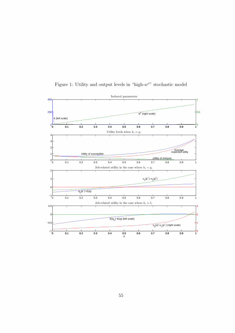
Figure 1: Utility and output levels in “high-we” stochastic model

0 0.1 0.2 0.3 0.4 0.5 0.6 0.7 0.8 0.9 10

200

400

k (left scale)

we (right scale)

Induced parameters

0 0.1 0.2 0.3 0.4 0.5 0.6 0.7 0.8 0.9 10

1

2

3

4

Utility of immune

Utility of susceptible

Averageexpected utility

Utility levels when ki = gi

0 0.1 0.2 0.3 0.4 0.5 0.6 0.7 0.8 0.9 1−1

0

1

2

q1(p−)−E(q)

u1(p−)−u

0(p*)

Job-related utility in the case where ki = gi

0 0.1 0.2 0.3 0.4 0.5 0.6 0.7 0.8 0.9 1−1

−0.5

0

0.5Job-related utility in the case where ki = `i

E(q1)−E(q) (left scale)

u0(v)−u

1(p−) (right scale)

α

0 0.1 0.2 0.3 0.4 0.5 0.6 0.7 0.8 0.9 10

0.5

1

0 0.1 0.2 0.3 0.4 0.5 0.6 0.7 0.8 0.9 10

1

2

3

55

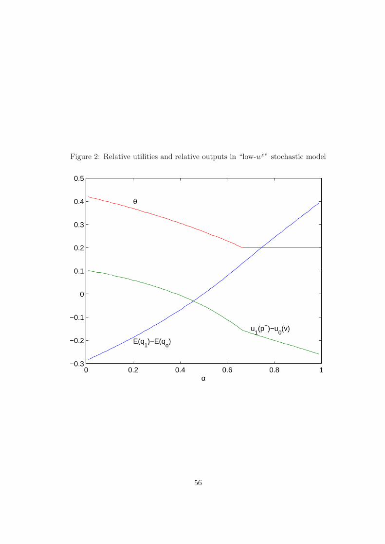
Figure 2: Relative utilities and relative outputs in “low-we” stochastic model

0 0.2 0.4 0.6 0.8 1−0.3

−0.2

−0.1

0

0.1

0.2

0.3

0.4

0.5

E(q1)−E(q

o)

α

θ

u1(p−)−u

0(v)

56