Peter W. Kimball and Stephen M. Rock

196 IEEE JOURNAL OF OCEANIC ENGINEERING, VOL. 40, NO. 1, JANUARY 2015

Mapping of Translating, Rotating Icebergs Withan Autonomous Underwater Vehicle

Peter W. Kimball and Stephen M. Rock

Abstract—This paper presents a method for mapping trans-lating, rotating icebergs with an autonomous underwater vehicle(AUV). To map an iceberg, the AUV first circumnavigates it,collecting multibeam sonar ranges and iceberg-relative Dopplersonar velocities from the submerged iceberg surface. The primarychallenge is then to estimate the trajectory of the mapping vehiclein a noninertial reference frame attached to the moving iceberg.The collected multibeam ranges may then be projected from thistrajectory to form a map of the iceberg's submerged surface. Theapproach of the method involves identifying the iceberg-framelocations of all the Doppler sonar measurements made duringcircumnavigation, allowing the AUV's iceberg-relative trajectoryto be computed from those locations. The measurement locationsare estimated simultaneously with the trajectory of the iceberg tobe most consistent with the inertial-space positions, inertial-spacevelocities, distances between points on the iceberg surface asmeasured by the Doppler sonar, and alignment of multibeamranges measured at the beginning and end of the circumnavi-gation. The measurements depend nonlinearly on the modeledpositions and iceberg trajectory, and the paper presents a solu-tion formulation that deals efficiently with the nonlinearity. Byincorporating iceberg-relative vehicle velocity into the estimation,the method achieves two significant advances beyond prior workby the authors. First, and most significantly, the method addsice-relative vehicle velocity measurements (e.g., using a Dopplervelocity logger). This makes the method robust to common vehicleinertial navigation errors. Second, inclusion of iceberg-relativevehicle velocity data allows for the identification of a more generalmodel of iceberg trajectory, making the method robust to changesin iceberg translation and rotation rates. Currently, no icebergcircumnavigation data sets are available that include iceberg-rel-ative velocity from Doppler sonar. However, this paper includesresults from simulated free-drifting icebergs, and experimentalresults from an AUV seafloor mapping dive. The simulationdata provide a moving iceberg testbed with known ground truthfor the mapping results. The seafloor data provide a qualitativeverification that the method works with real vehicle data.

Index Terms—Estimation , ice, marine navigation, marine vehi-cles, motion estimation, terrain mapping.

Manuscript received February 11, 2013; revised September 30, 2013; ac-cepted January 09, 2014. Date of publication February 21, 2014; date of currentversion January 09, 2015. This work was supported by the National ScienceFoundation and the National Aeronautics & Space Administration's Astrobi-ology Science and Technology for Exploring Planets Program.Associate Editor: R. Eustice.P.W. Kimball is with the Applied Ocean Physics & Engineering Department,

Woods Hole Oceanographic Institution, Woods Hole, MA USA (e-mail: [email protected]).S. M. Rock is with the Department of Aeronautics and Astronautics and the

Aerospace Robotics Laboratory, Stanford University, Stanford, CA 94305USA.Digital Object Identifier 10.1109/JOE.2014.2300396

I. INTRODUCTION

T HIS paper presents a technique for creating 3-D mapsof the submerged surfaces of free-drifting icebergs using

an autonomous underwater vehicle (AUV). There is growinginterest in the scientific community to understand the impactof large, free-drifting icebergs on ocean ecosystems and globalenergy processes. AUVs present an opportunity for very highspatial and temporal resolution sampling around icebergs(compared to other existing sampling techniques). Prior workhas identified maps of free-drifting icebergs as both an impor-tant scientific data product and an enabler of close-proximityiceberg-relative AUV navigation [12]. Existing AUV mappingtechniques are well developed for seafloor applications, butrequire extension to handle the noninertial motion (translationand rotation) of free-drifting icebergs.The map surface data in this application come from a multi-

beam sonar carried by a submerged AUV. As the AUV drivesaround an iceberg, this instrument collects a 2-D, cross-trackfan-shaped pattern of hundreds of range measurements from thevehicle to the iceberg's submerged surface once every 1–3 s.A map of the iceberg is formed by projecting these multibeamranges from a best estimate of the iceberg-relative vehicle po-sition and orientation at the time of each measurement, i.e., areconstructed vehicle trajectory in an iceberg-fixed frame. Thisreference frame is noninertial, translating and rotating with theiceberg. Estimating the AUV trajectory in this frame is the focusof this paper.Iceberg translation and rotation through inertial space are sig-

nificant during the time required for an AUV to travel around aniceberg and achieve multibeam sonar coverage. Iceberg transla-tional speeds of 0.03–0.08 m/s and rotation rates of 5–10 /h aretypical, while translational speeds up to 0.27 m/s and rotationrates up to 40 /h have been observed [18], [8]. Even for a rel-atively fast AUV with a nominal operating speed of 1.75 m/s,circumnavigating a small (1.8 km across) iceberg takes an hour.Typical iceberg motion over this time can result in 110–290m ofaccumulated displacement, and 5 –10 of orientation change.Prior iceberg mapping work by the authors [12] demonstrates

the need to account for iceberg motion to create self-consis-tent iceberg maps. It utilizes a simple, constant-translation, con-stant-rotation model of iceberg motion and identifies the param-eter values in the model only through loop closure in the multi-beam data, i.e., the translation and rotation rates are chosen tomaximize self-consistency in the map region ensonified both atthe beginning and end of the circumnavigation. That work doesnot include any direct measurements of iceberg-relative vehiclevelocity from Doppler sonar.

0364-9059 © 2014 IEEE. Personal use is permitted, but republication/redistribution requires IEEE permission.See http://www.ieee.org/publications_standards/publications/rights/index.html for more information.

KIMBALL AND ROCK: MAPPING OF TRANSLATING, ROTATING ICEBERGS WITH AN AUTONOMOUS UNDERWATER VEHICLE 197

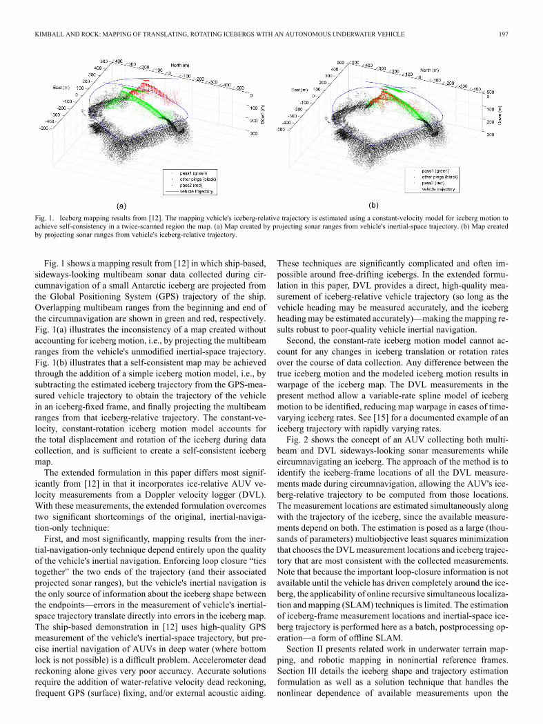
Fig. 1. Iceberg mapping results from [12]. The mapping vehicle's iceberg-relative trajectory is estimated using a constant-velocity model for iceberg motion toachieve self-consistency in a twice-scanned region the map. (a) Map created by projecting sonar ranges from vehicle's inertial-space trajectory. (b) Map createdby projecting sonar ranges from vehicle's iceberg-relative trajectory.

Fig. 1 shows a mapping result from [12] in which ship-based,sideways-looking multibeam sonar data collected during cir-cumnavigation of a small Antarctic iceberg are projected fromthe Global Positioning System (GPS) trajectory of the ship.Overlapping multibeam ranges from the beginning and end ofthe circumnavigation are shown in green and red, respectively.Fig. 1(a) illustrates the inconsistency of a map created withoutaccounting for iceberg motion, i.e., by projecting the multibeamranges from the vehicle's unmodified inertial-space trajectory.Fig. 1(b) illustrates that a self-consistent map may be achievedthrough the addition of a simple iceberg motion model, i.e., bysubtracting the estimated iceberg trajectory from the GPS-mea-sured vehicle trajectory to obtain the trajectory of the vehiclein an iceberg-fixed frame, and finally projecting the multibeamranges from that iceberg-relative trajectory. The constant-ve-locity, constant-rotation iceberg motion model accounts forthe total displacement and rotation of the iceberg during datacollection, and is sufficient to create a self-consistent icebergmap.The extended formulation in this paper differs most signif-

icantly from [12] in that it incorporates ice-relative AUV ve-locity measurements from a Doppler velocity logger (DVL).With these measurements, the extended formulation overcomestwo significant shortcomings of the original, inertial-naviga-tion-only technique:First, and most significantly, mapping results from the iner-

tial-navigation-only technique depend entirely upon the qualityof the vehicle's inertial navigation. Enforcing loop closure “tiestogether” the two ends of the trajectory (and their associatedprojected sonar ranges), but the vehicle's inertial navigation isthe only source of information about the iceberg shape betweenthe endpoints—errors in the measurement of vehicle's inertial-space trajectory translate directly into errors in the iceberg map.The ship-based demonstration in [12] uses high-quality GPSmeasurement of the vehicle's inertial-space trajectory, but pre-cise inertial navigation of AUVs in deep water (where bottomlock is not possible) is a difficult problem. Accelerometer deadreckoning alone gives very poor accuracy. Accurate solutionsrequire the addition of water-relative velocity dead reckoning,frequent GPS (surface) fixing, and/or external acoustic aiding.

These techniques are significantly complicated and often im-possible around free-drifting icebergs. In the extended formu-lation in this paper, DVL provides a direct, high-quality mea-surement of iceberg-relative vehicle trajectory (so long as thevehicle heading may be measured accurately, and the icebergheading may be estimated accurately)—making the mapping re-sults robust to poor-quality vehicle inertial navigation.Second, the constant-rate iceberg motion model cannot ac-

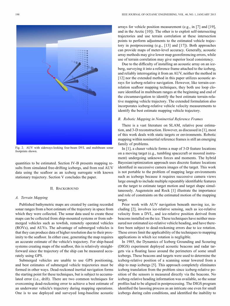
count for any changes in iceberg translation or rotation ratesover the course of data collection. Any difference between thetrue iceberg motion and the modeled iceberg motion results inwarpage of the iceberg map. The DVL measurements in thepresent method allow a variable-rate spline model of icebergmotion to be identified, reducing map warpage in cases of time-varying iceberg rates. See [15] for a documented example of aniceberg trajectory with rapidly varying rates.Fig. 2 shows the concept of an AUV collecting both multi-

beam and DVL sideways-looking sonar measurements whilecircumnavigating an iceberg. The approach of the method is toidentify the iceberg-frame locations of all the DVL measure-ments made during circumnavigation, allowing the AUV's ice-berg-relative trajectory to be computed from those locations.The measurement locations are estimated simultaneously alongwith the trajectory of the iceberg, since the available measure-ments depend on both. The estimation is posed as a large (thou-sands of parameters) multiobjective least squares minimizationthat chooses the DVLmeasurement locations and iceberg trajec-tory that are most consistent with the collected measurements.Note that because the important loop-closure information is notavailable until the vehicle has driven completely around the ice-berg, the applicability of online recursive simultaneous localiza-tion and mapping (SLAM) techniques is limited. The estimationof iceberg-frame measurement locations and inertial-space ice-berg trajectory is performed here as a batch, postprocessing op-eration—a form of offline SLAM.Section II presents related work in underwater terrain map-

ping, and robotic mapping in noninertial reference frames.Section III details the iceberg shape and trajectory estimationformulation as well as a solution technique that handles thenonlinear dependence of available measurements upon the


Fig. 2. AUV with sideways-looking four-beam DVL and multibeam sonarfootprints shown.

quantities to be estimated. Section IV-B presents mapping re-sults from simulated free-drifting icebergs, and from real AUVdata using the seafloor as an iceberg surrogate with knownstationary trajectory. Section V concludes the paper.

II. BACKGROUND

A. Terrain Mapping

Published bathymetric maps are created by casting recordedsonar ranges from a best estimate of the trajectory in space fromwhich they were collected. The sonar data used to create thesemaps can be collected from ship-mounted systems or from sub-merged vehicles such as towfish, remotely operated vehicles(ROVs), and AUVs. The advantage of submerged vehicles isthat they can produce data of higher resolution due to their prox-imity to the seafloor. In either case, generating the map requiresan accurate estimate of the vehicle's trajectory. For ship-basedsystems creating maps of the seafloor, this is relatively straight-forward since the trajectory of the ship can be measured accu-rately using GPS.Submerged vehicles are unable to use GPS positioning,

and best estimates of submerged vehicle trajectories must beformed in other ways. Dead-reckoned inertial navigation formsthe starting point for these techniques, but is subject to accumu-lated error (i.e., drift). There are two common techniques forovercoming dead-reckoning error to achieve a best estimate ofan underwater vehicle's trajectory during mapping operations.One is to use deployed and surveyed long-baseline acoustic

arrays for vehicle position measurement (e.g., in [7] and [19],and in the Arctic [10]). The other is to exploit self-intersectingtrajectories and use terrain correlation at these intersectionpoints to perform adjustments to the estimated vehicle trajec-tory in postprocessing (e.g., [13] and [17]). Both approachescan provide maps of meter-level accuracy. Generally, acousticarray methods may give lower map georeferencing errors, whileuse of terrain correlation may give superior local consistency.Due to the difficulty of installing an acoustic array on an ice-

berg, surveying it into a reference frame attached to the iceberg,and reliably interrogating it from an AUV, neither the method in[12] nor the extended method in this paper utilizes acoustic ar-rays for iceberg-relative navigation. However, like terrain-cor-relation seafloor mapping techniques, they both use loop clo-sure identified in multibeam ranges at the beginning and end ofthe circumnavigation to identify the best estimate terrain-rela-tive mapping vehicle trajectory. The extended formulation alsoincorporates iceberg-relative vehicle velocity measurements toidentify the best estimate mapping vehicle trajectory.

B. Robotic Mapping in Noninertial Reference Frames

There is a vast literature on SLAM, relative pose estima-tion, and 3-D reconstruction. However, as discussed in [1], mostof this work deals with static targets or environments. Roboticmapping within noninertial reference frames is still an emergingfamily of problems.In [1], a chaser vehicle forms a map of 3-D feature locations

on a moving target (e.g., tumbling spacecraft or moored instru-ment) undergoing unknown forces and moments. The hybridBayesian/optimization approach uses discrete feature locationsidentified in successive camera images of the target. This workis not portable to the problem of mapping large environmentssuch as icebergs because it requires successive camera viewslarge enough to include multiple repeatably identifiable featureson the target to estimate target motion and target shape simul-taneously. Augenstein and Rock [1] illustrate the importanceand role of constraints on the estimated motion of the mappingtarget.Prior work with AUV navigation beneath moving ice, in-

cluding [2], involves ice-relative sensing, such as ice-relativevelocity from a DVL, and ice-relative position derived frombeacons installed on the ice. These techniques have neither mea-sured nor estimated ice-relative vehicle heading, and have there-fore been subject to dead-reckoning errors due to ice rotation.These errors limit the applicability of the techniques to mappingapplications in which ice rotation is negligible.In 1985, the Dynamics of Iceberg Grounding and Scouring

(DIGS) experiment deployed acoustic beacons and radar tar-gets via a floating lasso around the perimeters of some smallicebergs. These beacons and targets were used to determine theiceberg-relative position of a scanning sonar lowered from aship to map icebergs [5]. This approach completely eliminatesiceberg translation from the problem since iceberg-relative po-sition of the sensors is measured directly via the beacons. Noiceberg-relative heading information was available, so the sonarprofiles had to be aligned in postprocessing. The DIGS programidentified the lassoing process as an intricate one even for smallicebergs during calm conditions, and identified the inability to


localize the transponders within the iceberg frame as a signifi-cant source of error.Only the prior work by the authors [12] and AUV-based up-

ward-looking sonar mapping of a rotating ice floe in [14] haverelied on both ice-relative and inertial sensing, accounting ex-plicitly for ice rotation in inertial space. In the latter, direct mea-surements of the ice floe's rotation and translation are obtainedvia the instrumentation of a ship moored to the floe during AUVoperations. Those measurements are included in a pose-graphformulation of the mapping problem which estimates both therotation of the floe and the floe-relative pose of the AUV at thetime of every multibeam measurement.The method presented in this work requires neither the instal-

lation of beacons on the iceberg nor the direct measurement oficeberg heading.

III. METHOD

A. Determining the Iceberg-Relative AUV Trajectory

The goal of the method is to estimate the mapping AUV'scircumnavigation trajectory in a frame attached to the movingiceberg. From this trajectory, the collected multibeam rangesmay be projected to form an iceberg map.Each DVL measurement consists of the range and Doppler

shift along each of four geometrically diverse beams (as inFig. 2). Most DVL applications involve computing a single3-D vehicle velocity based on the Doppler shifts measuredalong all four beams. This is understood as the velocity of thevehicle with respect to the seafloor in seafloor applications, andas the velocity of the vehicle with respect to the iceberg in thisapplication.Together with the vehicle's inertial-space velocity, the ice-

berg-relative velocity from DVL gives a measurement of theiceberg's inertial-space velocity. Because all points on the ice-berg are moving with different velocities through inertial space(due to rotation), any iceberg velocity measured in this wayapplies only to a single point on the iceberg surface. In thismethod, that point is located on a plane fit to the four returnlocations, and along a ray in the center of the four-beam con-stellation (similar to one common practice for computing alti-tude using bottom-tracking DVLs). This single point is referredto as a “DVL projected point” (DPP) in the remainder of thispaper. This approximation is only a very small source of errorsince the spread of the DVL beams is generally less than 50 m,a distance over which the difference in iceberg velocity due torotation is negligible.This method uses the iceberg-frame DPP locations and

control points in a spline model of inertial-space iceberg tra-jectory as intermediate variables. The method chooses theirvalues to maximize agreement with collected measurements,and then computes the iceberg-relative AUV trajectory fromthe estimated iceberg-frame DPP locations. Importantly, notall DVL measurements need to be assigned DPPs. As dis-cussed in Section III-D3, most DVL measurements are usedonly as iceberg-relative vehicle velocity measurements for

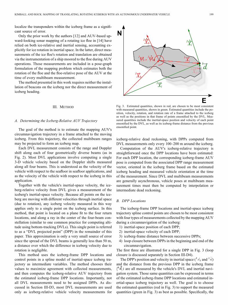
Fig. 3. Estimated quantities, shown in red, are chosen to be most consistentwith measured quantities, shown in green. Estimated quantities include the po-sition, velocity, rotation, and rotation rate of a frame attached to the icebergas well as the positions in that frame of points ensonified by the DVL. Mea-sured quantities include the inertial-space position and velocity of each pointensonified by the DVL, as well as its iceberg-frame distance from the previousensonified point.

iceberg-relative dead reckoning, with DPPs computed fromDVL measurements only every 100–200 m around the iceberg.Computation of the AUV's iceberg-relative trajectory is

straightforward once the DPP locations have been estimated:For each DPP location, the corresponding iceberg-frame AUVpose is computed from the associated DPP range measurementvector, oriented in the iceberg frame based on the estimatediceberg heading and measured vehicle orientation at the timeof the measurement. Since DVL and multibeam measurementsare generally asynchronous, vehicle poses at multibeam mea-surement times must then be computed by interpolation orintermediate dead reckoning.

B. DPP Locations

The iceberg-frame DPP locations and inertial-space icebergtrajectory spline control points are chosen to be most consistentwith four types of measurements collected by themapping AUVduring a circumnavigation of the iceberg:1) inertial-space position of each DPP;2) inertial-space velocity of each DPP;3) iceberg-frame distance between successive DPPs;4) loop closure between DPPs in the beginning and end of thecircumnavigation.

The first three are illustrated for a single DPP in Fig. 3 (loopclosure is discussed separately in Section III-D4).The DPP's position and velocity in inertial space ( and )

and the distance from the previous DPP in the iceberg frameare all measured by the vehicle's DVL and inertial navi-

gation system. Those same quantities can be expressed in termsof the estimated iceberg-frame DPP locations and estimated in-ertial-space iceberg trajectory as well. The goal is to choosethe estimated quantities (red in Fig. 3) to support the measuredquantities (green in Fig. 3) as best as possible. Specifically, the


estimated iceberg trajectory and DPP positions are chosen tominimize

(1)

Each term of the cost function represents the disagreementbetween the model and one type of collected measurement.contains the control points for the iceberg translational trajec-tory spline, and the iceberg-frame DPP locations. gives themodeled inertial-space DPP locations, and contains the mea-sured locations. gives the modeled inertial-space DPP ve-locities, and contains the measured velocities. gives themodeled iceberg-frame distance between DPPs, and containsthe measured (by DVL dead reckoning) iceberg-frame distancebetweenDPPs. encodes the loop-closure objective betweenrelevant DPPs from the beginning and end of the circumnavi-gation. Finally, gives solution uniqueness by expressing aframe-centering objective.The remainder of this section details the spline models used

to represent iceberg translation and rotation, the formulation ofthe measurement model matrices , and finally a minimizationtechnique which handles the nonlinearity of —specifically,that , , and all depend on the unknown iceberg heading.

C. Spline Model for Iceberg Trajectory

To facilitate accurate and tractable estimation of the icebergtrajectory, the model used to express the trajectory needs to de-scribe realistic iceberg motions using a small number of param-eters compared to the total number of DVL position and ve-locity measurements made during data collection. Specifically,this method uses splines to represent iceberg translation and ro-tation through inertial space. Splines are piecewise polynomialscomposed of weighted sums of basis functions in time. Theorder, number, and spacing of basis functions may be chosen.The weights are called control points, and have a geometric in-terpretation. See [16] for a full coverage of splines. While anumber of parametric forms (e.g., other piecewise polynomials,Fourier series) may be able to describe iceberg motion, splinesare used here for three reasons:1) splines are “well behaved” at their endpoints (versus e.g.,Taylor polynomials);

2) splines allow for the inclusion of physical constraints suchas continuous acceleration;

3) every position along a spline-modeled trajectory is a linearfunction of its control points.

This method uses one spline to represent the inertial-spacetrajectory taken by the origin of a reference frame attached tothe iceberg and another spline to represent the headingof that reference frame . Both of these splines are definedin time (over the duration of data collection), and specified by alinear combination of basis splines as in

(2)

(3)

The only free parameters in these models are the controlpoints and . For a given degree or , number ofcontrol points or , and knot spacing in time, each basisspline or is a fully defined function only oftime . Note that the position spline is vector valued, while theheading spline is scalar valued.An important property of the spline model is that both the

position and velocity of the iceberg frame are described as linearfunctions of the same control points. Specifically, at the time ofthe th measurement, the iceberg-frame position and translationrate are given by the matrix multiplications in

(4)

(5)

Importantly, the translational position and translational velocitysplines differ only in their known basis functions ( versus ),not in their control points.Here, is a stacked vector containing the 2-D (north,

east) control points for the position spline. Similarly, the mod-eled heading and heading rate of the iceberg are given by thematrix multiplications in

(6)

(7)

where is a stacked vector of the scalar heading spline controlpoints.A small number of parameters in and completely

define (through a linear model) the iceberg's translation andheading over the duration of data collection.The modeled trajectory passes through its first and last con-

trol points. The number of inflection points in each spline curveis limited by the number of basis splines (control points) com-posing the curve. So, as the number and degree of the basissplines in a spline grow, so does the space of functions whichthe spline can accurately represent. While there is no theoreticallimit on the number and degree of the basis splines used to forma spline, using more requires estimating the values of more con-trol points and it is best to use the simplest representation whichcan still represent accurately the true iceberg trajectory.The results in this paper use cubic basis splines with

quadruply repeated knots at the beginning and end of datacollection, and single knots at interior times, uniformly spacedin time by at most 1 h. This representation gives a spline trajec-tory of increasing complexity as the duration of data collectiongrows. Physically, the trajectory is restricted to continuous,


piecewise-linear acceleration. As a practical matter, qualita-tive observations of iceberg trajectory during data collection(e.g., known tidal current reversals, observed changes in windforcing) could be used to structure the spline, but simply addinguniformly spaced single knots as the duration of data collec-tion grows is a reliable approach with physical limitations, asdescribed above.

D. Measurement Model Matrices

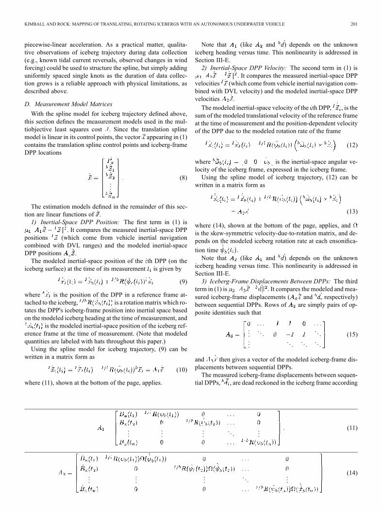
With the spline model for iceberg trajectory defined above,this section defines the measurement models used in the mul-tiobjective least squares cost . Since the translation splinemodel is linear in its control points, the vector appearing in (1)contains the translation spline control points and iceberg-frameDPP locations

...

(8)

The estimation models defined in the remainder of this sec-tion are linear functions of .1) Inertial-Space DPP Position: The first term in (1) is

. It compares the measured inertial-space DPPpositions (which come from vehicle inertial navigationcombined with DVL ranges) and the modeled inertial-spaceDPP positions .The modeled inertial-space position of the th DPP (on the

iceberg surface) at the time of its measurement is given by

(9)

where is the position of the DPP in a reference frame at-tached to the iceberg, is a rotationmatrix which ro-tates the DPP's iceberg-frame position into inertial space basedon the modeled iceberg heading at the time of measurement, and

is the modeled inertial-space position of the iceberg ref-erence frame at the time of measurement. (Note that modeledquantities are labeled with hats throughout this paper.)Using the spline model for iceberg trajectory, (9) can be

written in a matrix form as

(10)

where (11), shown at the bottom of the page, applies.

Note that (like and ) depends on the unknowniceberg heading versus time. This nonlinearity is addressed inSection III-E.2) Inertial-Space DPP Velocity: The second term in (1) is

. It compares the measured inertial-space DPPvelocities (which come from vehicle inertial navigation com-bined with DVL velocity) and the modeled inertial-space DPPvelocities .The modeled inertial-space velocity of the th DPP, , is the

sum of the modeled translational velocity of the reference frameat the time of measurement and the position-dependent velocityof the DPP due to the modeled rotation rate of the frame

(12)

where is the inertial-space angular ve-locity of the iceberg frame, expressed in the iceberg frame.Using the spline model of iceberg trajectory, (12) can be

written in a matrix form as

(13)

where (14), shown at the bottom of the page, applies, andis the skew-symmetric velocity-due-to-rotation matrix, and de-pends on the modeled iceberg rotation rate at each ensonifica-

tion time .Note that (like and ) depends on the unknown

iceberg heading versus time. This nonlinearity is addressed inSection III-E.3) Iceberg-Frame Displacements Between DPPs: The third

term in (1) is . It compares the modeled and mea-sured iceberg-frame displacements ( and , respectively)between sequential DPPs. Rows of are simply pairs of op-posite identities such that

.... . .

. . ....

. . .. . .

. . .

(15)

and then gives a vector of the modeled iceberg-frame dis-placements between sequential DPPs.The measured iceberg-frame displacements between sequen-

tial DPPs, , are dead reckoned in the iceberg frame according

......

.... . .

...(11)

......

.... . .

...(14)


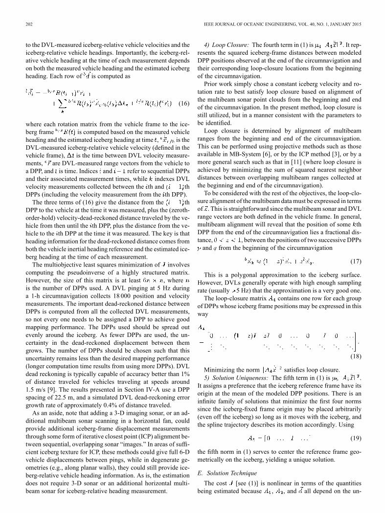
to the DVL-measured iceberg-relative vehicle velocities and theiceberg-relative vehicle headings. Importantly, the iceberg-rel-ative vehicle heading at the time of each measurement dependson both the measured vehicle heading and the estimated icebergheading. Each row of is computed as

(16)

where each rotation matrix from the vehicle frame to the ice-berg frame is computed based on the measured vehicleheading and the estimated iceberg heading at time , is theDVL-measured iceberg-relative vehicle velocity (defined in thevehicle frame), is the time between DVL velocity measure-ments, are DVL-measured range vectors from the vehicle toa DPP, and is time. Indices and refer to sequential DPPsand their associated measurement times, while indexes DVLvelocity measurements collected between the th and thDPPs (including the velocity measurement from the th DPP).The three terms of (16) give the distance from the th

DPP to the vehicle at the time it was measured, plus the (zeroth-order-hold) velocity-dead-reckoned distance traveled by the ve-hicle from then until the th DPP, plus the distance from the ve-hicle to the th DPP at the time it was measured. The key is thatheading information for the dead-reckoned distance comes fromboth the vehicle inertial heading reference and the estimated ice-berg heading at the time of each measurement.The multiobjective least squares minimization of involves

computing the pseudoinverse of a highly structured matrix.However, the size of this matrix is at least , whereis the number of DPPs used. A DVL pinging at 5 Hz duringa 1-h circumnavigation collects 18 000 position and velocitymeasurements. The important dead-reckoned distance betweenDPPs is computed from all the collected DVL measurements,so not every one needs to be assigned a DPP to achieve goodmapping performance. The DPPs used should be spread outevenly around the iceberg. As fewer DPPs are used, the un-certainty in the dead-reckoned displacement between themgrows. The number of DPPs should be chosen such that thisuncertainty remains less than the desired mapping performance(longer computation time results from using more DPPs). DVLdead reckoning is typically capable of accuracy better than 1%of distance traveled for vehicles traveling at speeds around1.5 m/s [9]. The results presented in Section IV-A use a DPPspacing of 22.5 m, and a simulated DVL dead-reckoning errorgrowth rate of approximately 0.4% of distance traveled.As an aside, note that adding a 3-D imaging sonar, or an ad-

ditional multibeam sonar scanning in a horizontal fan, couldprovide additional iceberg-frame displacement measurementsthrough some form of iterative closest point (ICP) alignment be-tween sequential, overlapping sonar “images.” In areas of suffi-cient iceberg texture for ICP, these methods could give full 6-Dvehicle displacements between pings, while in degenerate ge-ometries (e.g., along planar walls), they could still provide ice-berg-relative vehicle heading information. As is, the estimationdoes not require 3-D sonar or an additional horizontal multi-beam sonar for iceberg-relative heading measurement.

4) Loop Closure: The fourth term in (1) is . It rep-resents the squared iceberg-frame distances between modeledDPP positions observed at the end of the circumnavigation andtheir corresponding loop-closure locations from the beginningof the circumnavigation.Prior work simply chose a constant iceberg velocity and ro-

tation rate to best satisfy loop closure based on alignment ofthe multibeam sonar point clouds from the beginning and endof the circumnavigation. In the present method, loop closure isstill utilized, but in a manner consistent with the parameters tobe identified.Loop closure is determined by alignment of multibeam

ranges from the beginning and end of the circumnavigation.This can be performed using projective methods such as thoseavailable in MB-System [6], or by the ICP method [3], or by amore general search such as that in [11] (where loop closure isachieved by minimizing the sum of squared nearest neighbordistances between overlapping multibeam ranges collected atthe beginning and end of the circumnavigation).To be considered with the rest of the objectives, the loop-clo-

sure alignment of themultibeam datamust be expressed in termsof . This is straightforward since themultibeam sonar andDVLrange vectors are both defined in the vehicle frame. In general,multibeam alignment will reveal that the position of some thDPP from the end of the circumnavigation lies a fractional dis-tance, , between the positions of two successive DPPsand from the beginning of the circumnavigation

(17)

This is a polygonal approximation to the iceberg surface.However, DVLs generally operate with high enough samplingrate (usually 5 Hz) that the approximation is a very good one.The loop-closure matrix contains one row for each group

of DPPs whose iceberg frame positions may be expressed in thisway

.... . .

. . .. . .

. . .. . .

. . .. . .

. . .

(18)

Minimizing the norm satisfies loop closure.5) Solution Uniqueness: The fifth term in (1) is .

It assigns a preference that the iceberg reference frame have itsorigin at the mean of the modeled DPP positions. There is aninfinite family of solutions that minimize the first four normssince the iceberg-fixed frame origin may be placed arbitrarily(even off the iceberg) so long as it moves with the iceberg, andthe spline trajectory describes its motion accordingly. Using

(19)

the fifth norm in (1) serves to center the reference frame geo-metrically on the iceberg, yielding a unique solution.

E. Solution Technique

The cost [see (1)] is nonlinear in terms of the quantitiesbeing estimated because , , and all depend on the un-


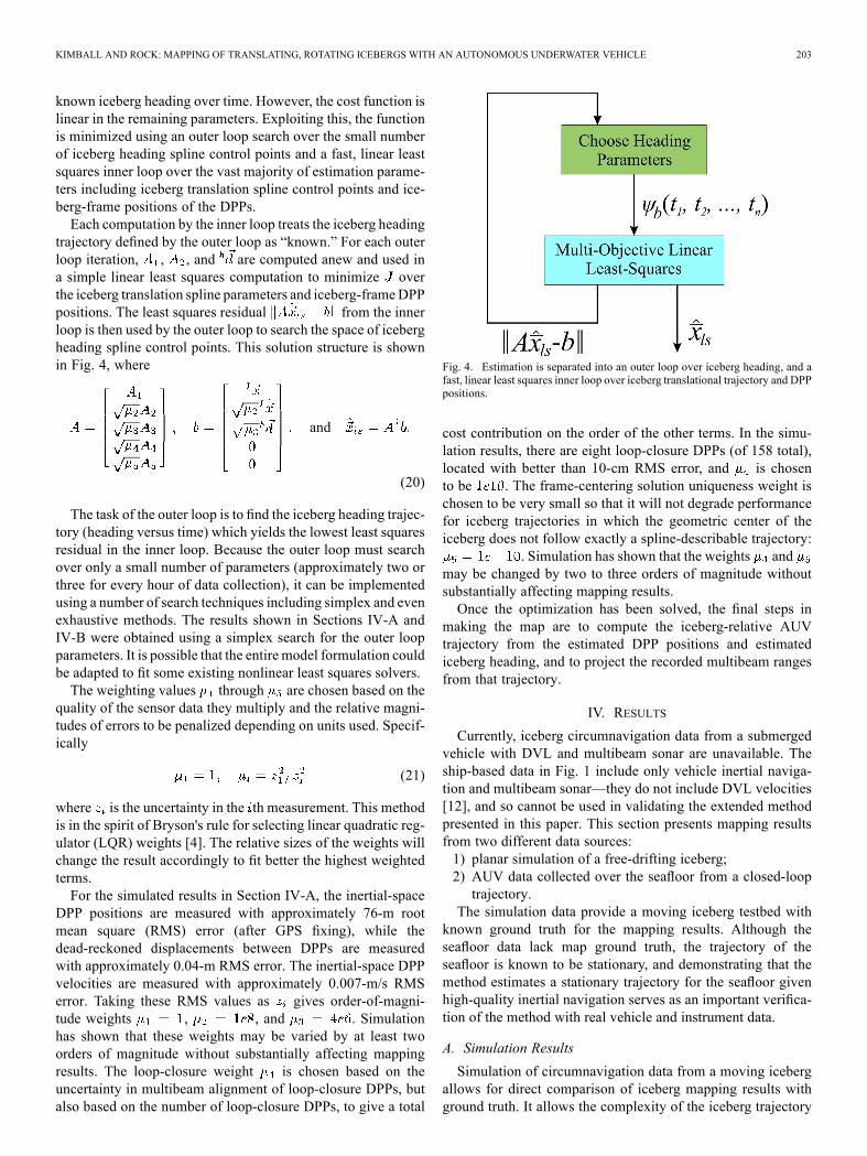
known iceberg heading over time. However, the cost function islinear in the remaining parameters. Exploiting this, the functionis minimized using an outer loop search over the small numberof iceberg heading spline control points and a fast, linear leastsquares inner loop over the vast majority of estimation parame-ters including iceberg translation spline control points and ice-berg-frame positions of the DPPs.Each computation by the inner loop treats the iceberg heading

trajectory defined by the outer loop as “known.” For each outerloop iteration, , , and are computed anew and used ina simple linear least squares computation to minimize overthe iceberg translation spline parameters and iceberg-frameDPPpositions. The least squares residual from the innerloop is then used by the outer loop to search the space of icebergheading spline control points. This solution structure is shownin Fig. 4, where

and

(20)

The task of the outer loop is to find the iceberg heading trajec-tory (heading versus time) which yields the lowest least squaresresidual in the inner loop. Because the outer loop must searchover only a small number of parameters (approximately two orthree for every hour of data collection), it can be implementedusing a number of search techniques including simplex and evenexhaustive methods. The results shown in Sections IV-A andIV-B were obtained using a simplex search for the outer loopparameters. It is possible that the entire model formulation couldbe adapted to fit some existing nonlinear least squares solvers.The weighting values through are chosen based on the

quality of the sensor data they multiply and the relative magni-tudes of errors to be penalized depending on units used. Specif-ically

(21)

where is the uncertainty in the th measurement. This methodis in the spirit of Bryson's rule for selecting linear quadratic reg-ulator (LQR) weights [4]. The relative sizes of the weights willchange the result accordingly to fit better the highest weightedterms.For the simulated results in Section IV-A, the inertial-space

DPP positions are measured with approximately 76-m rootmean square (RMS) error (after GPS fixing), while thedead-reckoned displacements between DPPs are measuredwith approximately 0.04-m RMS error. The inertial-space DPPvelocities are measured with approximately 0.007-m/s RMSerror. Taking these RMS values as gives order-of-magni-tude weights , , and . Simulationhas shown that these weights may be varied by at least twoorders of magnitude without substantially affecting mappingresults. The loop-closure weight is chosen based on theuncertainty in multibeam alignment of loop-closure DPPs, butalso based on the number of loop-closure DPPs, to give a total

Fig. 4. Estimation is separated into an outer loop over iceberg heading, and afast, linear least squares inner loop over iceberg translational trajectory and DPPpositions.

cost contribution on the order of the other terms. In the simu-lation results, there are eight loop-closure DPPs (of 158 total),located with better than 10-cm RMS error, and is chosento be . The frame-centering solution uniqueness weight ischosen to be very small so that it will not degrade performancefor iceberg trajectories in which the geometric center of theiceberg does not follow exactly a spline-describable trajectory:

. Simulation has shown that the weights andmay be changed by two to three orders of magnitude withoutsubstantially affecting mapping results.Once the optimization has been solved, the final steps in

making the map are to compute the iceberg-relative AUVtrajectory from the estimated DPP positions and estimatediceberg heading, and to project the recorded multibeam rangesfrom that trajectory.

IV. RESULTS

Currently, iceberg circumnavigation data from a submergedvehicle with DVL and multibeam sonar are unavailable. Theship-based data in Fig. 1 include only vehicle inertial naviga-tion and multibeam sonar—they do not include DVL velocities[12], and so cannot be used in validating the extended methodpresented in this paper. This section presents mapping resultsfrom two different data sources:1) planar simulation of a free-drifting iceberg;2) AUV data collected over the seafloor from a closed-looptrajectory.

The simulation data provide a moving iceberg testbed withknown ground truth for the mapping results. Although theseafloor data lack map ground truth, the trajectory of theseafloor is known to be stationary, and demonstrating that themethod estimates a stationary trajectory for the seafloor givenhigh-quality inertial navigation serves as an important verifica-tion of the method with real vehicle and instrument data.

A. Simulation Results

Simulation of circumnavigation data from a moving icebergallows for direct comparison of iceberg mapping results withground truth. It allows the complexity of the iceberg trajectory


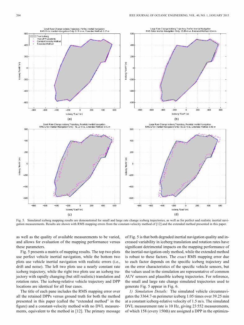
Fig. 5. Simulated iceberg mapping results are demonstrated for small and large rate change iceberg trajectories, as well as for perfect and realistic inertial navi-gation measurements. Results are shown with RMS mapping errors from the constant-velocity method of [12] and the extended method presented in this paper.

as well as the quality of available measurements to be varied,and allows for evaluation of the mapping performance versusthese parameters.Fig. 5 presents a matrix of mapping results. The top two plots

use perfect vehicle inertial navigation, while the bottom twoplots use vehicle inertial navigation with realistic errors (i.e.,drift and noise). The left two plots use a nearly constant rateiceberg trajectory, while the right two plots use an iceberg tra-jectory with rapidly changing (but still realistic) translation androtation rates. The iceberg-relative vehicle trajectory and DPPlocations are identical for all four cases.The title of each pane includes the RMS mapping error over

all the retained DPPs versus ground truth for both the methodpresented in this paper (called the “extended method” in thefigure) and a constant-velocity method with no DVL measure-ments, equivalent to the method in [12]. The primary message

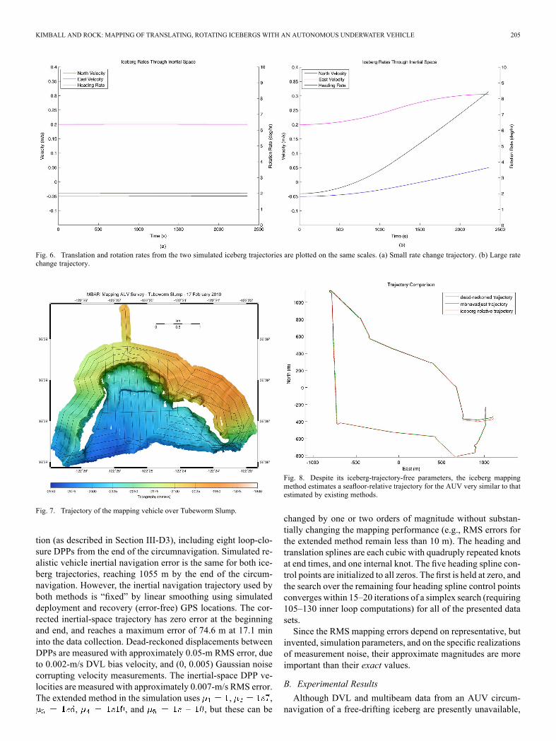
of Fig. 5 is that both degraded inertial navigation quality and in-creased variability in iceberg translation and rotation rates havesignificant detrimental impacts on the mapping performance ofthe inertial-navigation-only method, while the extended methodis robust to these factors. The exact RMS mapping error dueto each factor depends on the specific iceberg trajectory andon the error characteristics of the specific vehicle sensors, butthe values used in the simulation are representative of commonAUV sensors and plausible iceberg trajectories. For reference,the small and large rate change simulated trajectories used togenerate Fig. 5 appear in Fig. 6.1) Simulation Details: The simulated vehicle circumnavi-

gates the 3364.7-m perimeter iceberg 1.05 times over 39.25 minat a constant iceberg-relative velocity of 1.5 m/s. The simulatedDVL measurement rate is 10 Hz, giving 23 552 measurements,of which 158 (every 150th) are assigned a DPP in the optimiza-


Fig. 6. Translation and rotation rates from the two simulated iceberg trajectories are plotted on the same scales. (a) Small rate change trajectory. (b) Large ratechange trajectory.

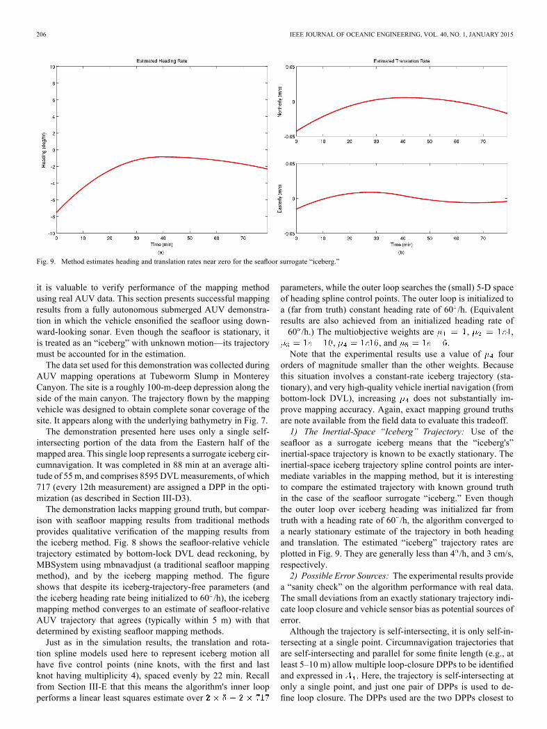
Fig. 7. Trajectory of the mapping vehicle over Tubeworm Slump.

tion (as described in Section III-D3), including eight loop-clo-sure DPPs from the end of the circumnavigation. Simulated re-alistic vehicle inertial navigation error is the same for both ice-berg trajectories, reaching 1055 m by the end of the circum-navigation. However, the inertial navigation trajectory used byboth methods is “fixed” by linear smoothing using simulateddeployment and recovery (error-free) GPS locations. The cor-rected inertial-space trajectory has zero error at the beginningand end, and reaches a maximum error of 74.6 m at 17.1 mininto the data collection. Dead-reckoned displacements betweenDPPs are measured with approximately 0.05-m RMS error, dueto 0.002-m/s DVL bias velocity, and (0, 0.005) Gaussian noisecorrupting velocity measurements. The inertial-space DPP ve-locities are measured with approximately 0.007-m/s RMS error.The extended method in the simulation uses , ,

, , and , but these can be

Fig. 8. Despite its iceberg-trajectory-free parameters, the iceberg mappingmethod estimates a seafloor-relative trajectory for the AUV very similar to thatestimated by existing methods.

changed by one or two orders of magnitude without substan-tially changing the mapping performance (e.g., RMS errors forthe extended method remain less than 10 m). The heading andtranslation splines are each cubic with quadruply repeated knotsat end times, and one internal knot. The five heading spline con-trol points are initialized to all zeros. The first is held at zero, andthe search over the remaining four heading spline control pointsconverges within 15–20 iterations of a simplex search (requiring105–130 inner loop computations) for all of the presented datasets.Since the RMS mapping errors depend on representative, but

invented, simulation parameters, and on the specific realizationsof measurement noise, their approximate magnitudes are moreimportant than their exact values.

B. Experimental Results

Although DVL and multibeam data from an AUV circum-navigation of a free-drifting iceberg are presently unavailable,


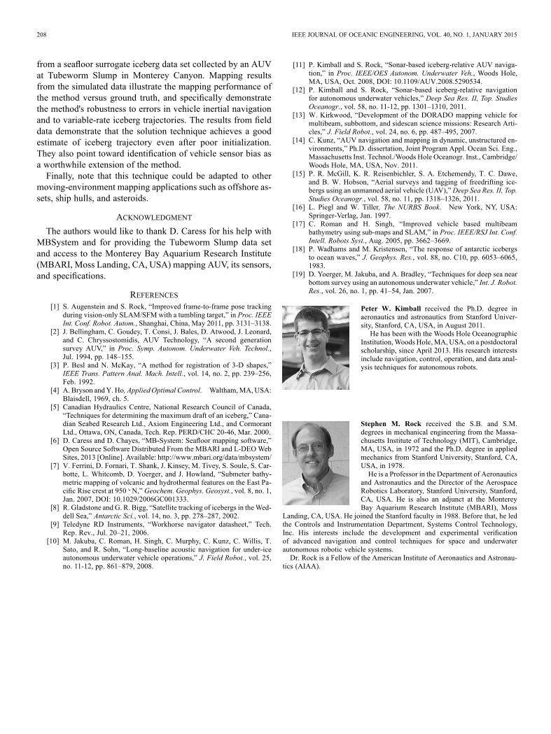
Fig. 9. Method estimates heading and translation rates near zero for the seafloor surrogate “iceberg.”

it is valuable to verify performance of the mapping methodusing real AUV data. This section presents successful mappingresults from a fully autonomous submerged AUV demonstra-tion in which the vehicle ensonified the seafloor using down-ward-looking sonar. Even though the seafloor is stationary, itis treated as an “iceberg” with unknown motion—its trajectorymust be accounted for in the estimation.The data set used for this demonstration was collected during

AUV mapping operations at Tubeworm Slump in MontereyCanyon. The site is a roughly 100-m-deep depression along theside of the main canyon. The trajectory flown by the mappingvehicle was designed to obtain complete sonar coverage of thesite. It appears along with the underlying bathymetry in Fig. 7.The demonstration presented here uses only a single self-

intersecting portion of the data from the Eastern half of themapped area. This single loop represents a surrogate iceberg cir-cumnavigation. It was completed in 88 min at an average alti-tude of 55m, and comprises 8595 DVLmeasurements, of which717 (every 12th measurement) are assigned a DPP in the opti-mization (as described in Section III-D3).The demonstration lacks mapping ground truth, but compar-

ison with seafloor mapping results from traditional methodsprovides qualitative verification of the mapping results fromthe iceberg method. Fig. 8 shows the seafloor-relative vehicletrajectory estimated by bottom-lock DVL dead reckoning, byMBSystem using mbnavadjust (a traditional seafloor mappingmethod), and by the iceberg mapping method. The figureshows that despite its iceberg-trajectory-free parameters (andthe iceberg heading rate being initialized to 60 /h), the icebergmapping method converges to an estimate of seafloor-relativeAUV trajectory that agrees (typically within 5 m) with thatdetermined by existing seafloor mapping methods.Just as in the simulation results, the translation and rota-

tion spline models used here to represent iceberg motion allhave five control points (nine knots, with the first and lastknot having multiplicity 4), spaced evenly by 22 min. Recallfrom Section III-E that this means the algorithm's inner loopperforms a linear least squares estimate over

parameters, while the outer loop searches the (small) 5-D spaceof heading spline control points. The outer loop is initialized toa (far from truth) constant heading rate of 60 /h. (Equivalentresults are also achieved from an initialized heading rate of60 /h.) The multiobjective weights are , ,

, , and .Note that the experimental results use a value of four

orders of magnitude smaller than the other weights. Becausethis situation involves a constant-rate iceberg trajectory (sta-tionary), and very high-quality vehicle inertial navigation (frombottom-lock DVL), increasing does not substantially im-prove mapping accuracy. Again, exact mapping ground truthsare note available from the field data to evaluate this tradeoff.1) The Inertial-Space “Iceberg” Trajectory: Use of the

seafloor as a surrogate iceberg means that the “iceberg's”inertial-space trajectory is known to be exactly stationary. Theinertial-space iceberg trajectory spline control points are inter-mediate variables in the mapping method, but it is interestingto compare the estimated trajectory with known ground truthin the case of the seafloor surrogate “iceberg.” Even thoughthe outer loop over iceberg heading was initialized far fromtruth with a heading rate of 60 /h, the algorithm converged toa nearly stationary estimate of the trajectory in both headingand translation. The estimated “iceberg” trajectory rates areplotted in Fig. 9. They are generally less than 4 /h, and 3 cm/s,respectively.2) Possible Error Sources: The experimental results provide

a “sanity check” on the algorithm performance with real data.The small deviations from an exactly stationary trajectory indi-cate loop closure and vehicle sensor bias as potential sources oferror.Although the trajectory is self-intersecting, it is only self-in-

tersecting at a single point. Circumnavigation trajectories thatare self-intersecting and parallel for some finite length (e.g., atleast 5–10 m) allow multiple loop-closure DPPs to be identifiedand expressed in . Here, the trajectory is self-intersecting atonly a single point, and just one pair of DPPs is used to de-fine loop closure. The DPPs used are the two DPPs closest to


Fig. 10. Inertial-space DPP velocities are shown (a) without and (b) with DVL bias correction. Since the seafloor is known to be stationary, these data should bezero-mean.

one another in inertial space from the beginning and end of thecircumnavigation. Further, since the beginning and end of thetrajectory are approximately orthogonal, the formulation ofas described in Section III-D4 is inappropriate for this data set.Here, is implemented as one block row of all zeros otherthan two opposite identities, one for each of the two loop-clo-sure DPPs. This is a source of error since those two DPP loca-tions actually lie several meters apart on the seafloor. couldbe reformulated to express loop closure at a single intersectionpoint exactly, but that point would be ill-defined for parallel,overlapping trajectory segments (such as those along a verticalface, passed twice at constant depth and standoff distance).Expressed in the vehicle frame, the measured inertial-space

DPP velocities are not zero mean, but are nearly constantmean. The mean magnitudes are 0.0039 m/s in vehiclefore/aft, 0.0029 m/s in vehicle starboard/port, and 0.0023m/s in vehicle down/up. These velocities are consistent withtypical DVL bias velocities (e.g., [9]), and subtracting thesevalues from the raw measured velocities before they are rotatedinto inertial space for use in the mapping method improvesestimation performance.Fig. 10 shows in green , the measured inertial-space

DPP velocities expressed in inertial space, without and withthe simple correction by vehicle-frame bias subtraction. Notethat the sudden change in mean apparent in the uncorrectedvelocities is not apparent in the corrected measured velocities.The solid red curve connects the estimated inertial-space DPPvelocities , and shows how well the model matches themeasurements for this one objective. Estimated iceberg ratesusing the bias-corrected inertial-space velocities are roughlyhalf of those shown in Fig. 9—generally less than 2 /h inheading, and 1.5 cm/s in translation.The bias velocity correction as performed here is possible be-

cause the terrain is known in advance to be stationary. How-ever, it indicates gains to be had from a slight reformulation ofthe estimation routine to include vehicle-frame bias velocitiesas parameters to be estimated. Operationally, this may requiremaneuvers during data acquisition to ensure observability of thebias rates.

Biases in other sensors (e.g., compass calibration), and errorsin their installation offsets (e.g., used in lever corrections, andframe rotations) represent additional sources of error in the post-processing solution not accounted for in the method.

V. SUMMARY AND CONCLUSION

This paper presents a technique for mapping a moving ice-berg using an AUV. The key technical feature of the work is amethod for estimating simultaneously the translation, rotation,and shape of an iceberg based on typical mapping data collectedduring a circumnavigation.The method uses splines to parameterize both the translation

and heading trajectories of the iceberg. The orders of the splinesas well as the numbers of control points used to define themmay be varied to describe iceberg motion up to physically mean-ingful constraints such as continuous piecewise-linear acceler-ation, and a maximum number of inflection points in icebergtrajectory.The method chooses simultaneously spline control point

values and the locations of DVL measurements in an ice-berg-fixed reference frame to maximize consistency withcollected data. The data include inertial-space positions andvelocities of points on the iceberg surface (from DVL rangesand velocities, and vehicle inertial navigation), iceberg-framedisplacements between DVL measurements, and loop-closurebetween the beginning and end of data collection (from over-lapping sets of multibeam sonar ranges).Modeled values of the collected data are nonlinear in iceberg

heading spline parameters, but linear in the iceberg translationspline parameters and in the iceberg-frame measurement loca-tions. To find the best estimate, an outer loop performs an iter-ative search over the relatively small space (on the order of tendimensions) of heading trajectory spline control points, whilea fast, linear least squares inner loop calculation solves for theoptimal values of the iceberg translation spline control pointsand iceberg-frame DVL measurement locations (on the order oftens of thousands of dimensions).In addition to the method itself, the paper presents mapping

results from simulated free-drifting iceberg data as well as


from a seafloor surrogate iceberg data set collected by an AUVat Tubeworm Slump in Monterey Canyon. Mapping resultsfrom the simulated data illustrate the mapping performance ofthe method versus ground truth, and specifically demonstratethe method's robustness to errors in vehicle inertial navigationand to variable-rate iceberg trajectories. The results from fielddata demonstrate that the solution technique achieves a goodestimate of iceberg trajectory even after poor initialization.They also point toward identification of vehicle sensor bias asa worthwhile extension of the method.Finally, note that this technique could be adapted to other

moving-environment mapping applications such as offshore as-sets, ship hulls, and asteroids.

ACKNOWLEDGMENT

The authors would like to thank D. Caress for his help withMBSystem and for providing the Tubeworm Slump data setand access to the Monterey Bay Aquarium Research Institute(MBARI, Moss Landing, CA, USA) mapping AUV, its sensors,and specifications.

REFERENCES[1] S. Augenstein and S. Rock, “Improved frame-to-frame pose tracking

during vision-only SLAM/SFM with a tumbling target,” in Proc. IEEEInt. Conf. Robot. Autom., Shanghai, China, May 2011, pp. 3131–3138.

[2] J. Bellingham, C. Goudey, T. Consi, J. Bales, D. Atwood, J. Leonard,and C. Chryssostomidis, AUV Technology, “A second generationsurvey AUV,” in Proc. Symp. Autonom. Underwater Veh. Technol.,Jul. 1994, pp. 148–155.

[3] P. Besl and N. McKay, “A method for registration of 3-D shapes,”IEEE Trans. Pattern Anal. Mach. Intell., vol. 14, no. 2, pp. 239–256,Feb. 1992.

[4] A. Bryson andY. Ho, AppliedOptimal Control. Waltham,MA,USA:Blaisdell, 1969, ch. 5.

[5] Canadian Hydraulics Centre, National Research Council of Canada,“Techniques for determining the maximum draft of an iceberg,” Cana-dian Seabed Research Ltd., Axiom Engineering Ltd., and CormorantLtd., Ottawa, ON, Canada, Tech. Rep. PERD/CHC 20-46, Mar. 2000.

[6] D. Caress and D. Chayes, “MB-System: Seafloor mapping software,”Open Source Software Distributed From the MBARI and L-DEOWebSites, 2013 [Online]. Available: http://www.mbari.org/data/mbsystem/

[7] V. Ferrini, D. Fornari, T. Shank, J. Kinsey, M. Tivey, S. Soule, S. Car-botte, L. Whitcomb, D. Yoerger, and J. Howland, “Submeter bathy-metric mapping of volcanic and hydrothermal features on the East Pa-cific Rise crest at 950 N,” Geochem. Geophys. Geosyst., vol. 8, no. 1,Jan. 2007, DOI: 10.1029/2006GC001333.

[8] R. Gladstone and G. R. Bigg, “Satellite tracking of icebergs in theWed-dell Sea,” Antarctic Sci., vol. 14, no. 3, pp. 278–287, 2002.

[9] Teledyne RD Instruments, “Workhorse navigator datasheet,” Tech.Rep. Rev., Jul. 20–21, 2006.

[10] M. Jakuba, C. Roman, H. Singh, C. Murphy, C. Kunz, C. Willis, T.Sato, and R. Sohn, “Long-baseline acoustic navigation for under-iceautonomous underwater vehicle operations,” J. Field Robot., vol. 25,no. 11-12, pp. 861–879, 2008.

[11] P. Kimball and S. Rock, “Sonar-based iceberg-relative AUV naviga-tion,” in Proc. IEEE/OES Autonom. Underwater Veh., Woods Hole,MA, USA, Oct. 2008, DOI: 10.1109/AUV.2008.5290534.

[12] P. Kimball and S. Rock, “Sonar-based iceberg-relative navigationfor autonomous underwater vehicles,” Deep Sea Res. II, Top. StudiesOceanogr., vol. 58, no. 11-12, pp. 1301–1310, 2011.

[13] W. Kirkwood, “Development of the DORADO mapping vehicle formultibeam, subbottom, and sidescan science missions: Research Arti-cles,” J. Field Robot., vol. 24, no. 6, pp. 487–495, 2007.

[14] C. Kunz, “AUV navigation and mapping in dynamic, unstructured en-vironments,” Ph.D. dissertation, Joint Program Appl. Ocean Sci. Eng.,Massachusetts Inst. Technol./Woods Hole Oceanogr. Inst., Cambridge/Woods Hole, MA, USA, Nov. 2011.

[15] P. R. McGill, K. R. Reisenbichler, S. A. Etchemendy, T. C. Dawe,and B. W. Hobson, “Aerial surveys and tagging of freedrifting ice-bergs using an unmanned aerial vehicle (UAV),”Deep Sea Res. II, Top.Studies Oceanogr., vol. 58, no. 11, pp. 1318–1326, 2011.

[16] L. Piegl and W. Tiller, The NURBS Book. New York, NY, USA:Springer-Verlag, Jan. 1997.

[17] C. Roman and H. Singh, “Improved vehicle based multibeambathymetry using sub-maps and SLAM,” in Proc. IEEE/RSJ Int. Conf.Intell. Robots Syst., Aug. 2005, pp. 3662–3669.

[18] P. Wadhams and M. Kristensen, “The response of antarctic icebergsto ocean waves,” J. Geophys. Res., vol. 88, no. C10, pp. 6053–6065,1983.

[19] D. Yoerger, M. Jakuba, and A. Bradley, “Techniques for deep sea nearbottom survey using an autonomous underwater vehicle,” Int. J. Robot.Res., vol. 26, no. 1, pp. 41–54, Jan. 2007.

Peter W. Kimball received the Ph.D. degree inaeronautics and astronautics from Stanford Univer-sity, Stanford, CA, USA, in August 2011.He has been with the Woods Hole Oceanographic

Institution,WoodsHole,MA,USA, on a postdoctoralscholarship, since April 2013. His research interestsinclude navigation, control, operation, and data anal-ysis techniques for autonomous robots.

Stephen M. Rock received the S.B. and S.M.degrees in mechanical engineering from the Massa-chusetts Institute of Technology (MIT), Cambridge,MA, USA, in 1972 and the Ph.D. degree in appliedmechanics from Stanford University, Stanford, CA,USA, in 1978.He is a Professor in the Department of Aeronautics

and Astronautics and the Director of the AerospaceRobotics Laboratory, Stanford University, Stanford,CA, USA. He is also an adjunct at the MontereyBay Aquarium Research Institute (MBARI), Moss

Landing, CA, USA. He joined the Stanford faculty in 1988. Before that, he ledthe Controls and Instrumentation Department, Systems Control Technology,Inc. His interests include the development and experimental verificationof advanced navigation and control techniques for space and underwaterautonomous robotic vehicle systems.Dr. Rock is a Fellow of the American Institute of Aeronautics and Astronau-

tics (AIAA).

Documents

Peter W. Kimball and Stephen M. Rock