Phased Array Antennas - Real Observatorio · DTSC-UC3M Page 2 06/02/2007 . Issues on Array Antennas 1. Introduction The very first step when we seek for the understanding of phased

Important issues on array antennas SKADS-DS4-T4

IT-OAN 2007 – 2

Eloy de Lera, J.A.López Fernández, J.M.Serna Puente, Roberto García

L.E.García (Univ. Carlos III)

Centro Astronómico de Yebes Aptdo. 148 19080 Guadalajara

SPAIN Phone: +34949290311 Fax: +34949290063

Issues on Array Antennas

Index

1. Introduction - 3

2. Classical Array Theory - 4

3. The Active Reflection Coefficient - 6 3.1 Array Pattern and the Active Reflection Coefficient - 9

4. Edge Effect - 13 4.1 Edge Elements ARC approximation - 14

5. Some more issues about Array Antennas - 19 5.1 Array Symmetries - 19

5.2 Simulations - 19

5.3 The UWB case - 20

6. Future Lines - 25

7. Conclusions - 26

8. References - 27

Appendices - 28

Appendix 1: Mutual Coupling Edge Effect Approximation for Phased-Array Antennas

DTSC-UC3M Page 2 06/02/2007


1. Introduction The very first step when we seek for the understanding of phased array antennas is the study of these systems in the ideal case, in a classical way [1], and this will be the first point of the document. The rest of the text will be dedicated to present and analyze some of the causes of the displacement between this ideal case and the real world. One of these causes is the mutual coupling [2]. Mutual coupling is the electromagnetic contribution of an excited antenna (transmission or reception are equivalent) to any other antenna in its surroundings. It is essential to understand where does this coupling come from, how much does it affect, which parameters may help to control its effect and of course, how can we compute it and relate it to the rest of classical parameters of an antenna system.



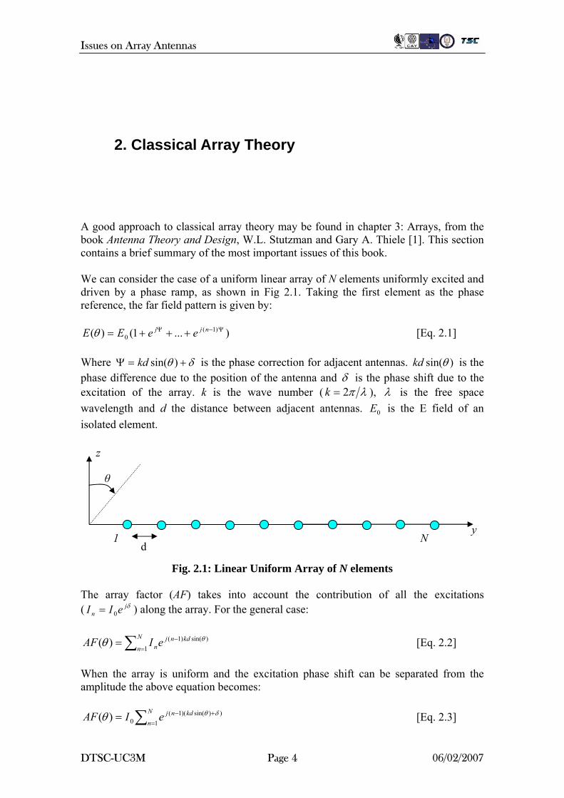
2. Classical Array Theory

A good approach to classical array theory may be found in chapter 3: Arrays, from the book Antenna Theory and Design, W.L. Stutzman and Gary A. Thiele [1]. This section contains a brief summary of the most important issues of this book. We can consider the case of a uniform linear array of N elements uniformly excited and driven by a phase ramp, as shown in Fig 2.1. Taking the first element as the phase reference, the far field pattern is given by:

)...1()( )1(0

Ψ−Ψ +++= njj eeEE θ [Eq. 2.1] Where δθ +=Ψ )sin(kd is the phase correction for adjacent antennas. )sin(θkd is the phase difference due to the position of the antenna and δ is the phase shift due to the excitation of the array. k is the wave number ( λπ2=k ), λ is the free space wavelength and d the distance between adjacent antennas. is the E field of an isolated element.

0E

y N

z

θ

1

The array ( )δj

n eII 0=

∑=AF )(θ When the aamplitude th

= IAF 0)(θ

DTSC-UC3

d

Fig. 2.1: Linear Uniform Array of N elements

factor (AF) takes into account the contribution of all the excitations along the array. For the general case:

=−N

nkdnj

neI1

)sin()1( θ [Eq. 2.2]

rray is uniform and the excitation phase shift can be separated from the e above equation becomes:

∑ =+−N

nkdnje

1))sin()(1( δθ [Eq. 2.3]

M Page 4 06/02/2007


The absolute value of this sum is:

)2/sin()2/sin()( 0 Ψ

Ψ=Ψ

NIAF [Eq. 2.4]

This expression is maximum for Ψ = 0 and the maximum value is NI0. Dividing this into Eq. 2.4 gives the normalized array factor:

)2/sin()2/sin()(

ΨΨ

=ΨN

Nf [Eq. 2.5]

This formulation let us calculate the maximum of the normalized array factor absolute value (the pointing direction of the array). But some other points need to be remarked first:

• The minor lobes are of width 2π/N in Ψ and the grating and mayor lobes twice this width.

• SLL: |Maximum value of largest side lobe|/|Maximum value of main lobe| decreases with N.

• The main lobe narrows as N increases. • There are N-2 side lobes and 1 main lobe in each period of Ψ (2π). • |f(Ψ)| is symmetric about π.

The θ pointing direction of a uniform linear array is:

)(sin)sin(0)sin( 1 kdkdkd δθθδδθ −=→−=→=+=Ψ − [Eq. 2.6] This equation is also useful for finding the phase ramp which produces a main lobe in the desired direction. At multiples of 2π in Ψ appear the undesired grating lobes, of same size than the main lobe. The number of these grating lobes increases as kd increases. It is a very important problem for wide band arrays, because the spacing d must be suitable (kd < 2π) for high frequencies (k big) in order to avoid the grating lobes and therefore the low frequencies will suffer from a very closely spaced array. This brings about some issues as the main beam widening. In the case of planar arrays (MxN elements – x and y directions) everything remains the same but the AF becomes:

∑∑ =−

=−=

M

mkxmj

xmN

nkynj

ynmn eIeIAF

1)cos()sin()1(

1)sin()sin()1(),( φθφθφθ [Eq. 2.7]

xm and yn are the distances between adjacent elements along x and y directions respectively.



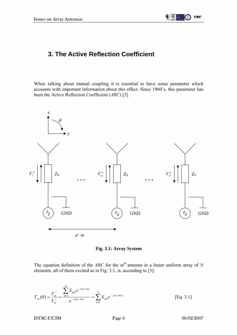
3. The Active Reflection Coefficient When talking about mutual coupling it is essential to have some parameter which accounts with important information about this effect. Since 1960’s, this parameter has been the Active Reflection Coefficient (ARC) [3]. z

θ y

GND

±1V Z0

GND

Z0 ±

mV

md ⋅

… …±

NV Z0

GND

Fig. 3.1: Array System

The equation definition of the ARC for the mth antenna in a linear uniform array of N elements, all of them excited as in Fig. 3.1, is, according to [3]:

∑∑

=

−−−−

=

−−

+

−

===ΓN

n

umnjmnumj

N

n

unjmn

m

mm eS

e

eS

VV

1

)()1(

1

)1(

)(θ [Eq. 3.1]



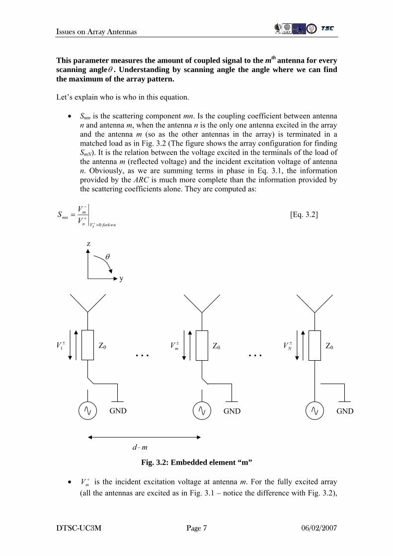
This parameter measures the amount of coupled signal to the mth antenna for every scanning angleθ . Understanding by scanning angle the angle where we can find the maximum of the array pattern. Let’s explain who is who in this equation.

• Smn is the scattering component mn. Is the coupling coefficient between antenna n and antenna m, when the antenna n is the only one antenna excited in the array and the antenna m (so as the other antennas in the array) is terminated in a matched load as in Fig. 3.2 (The figure shows the array configuration for finding SmN). It is the relation between the voltage excited in the terminals of the load of the antenna m (reflected voltage) and the incident excitation voltage of antenna n. Obviously, as we are summing terms in phase in Eq. 3.1, the information provided by the ARC is much more complete than the information provided by the scattering coefficients alone. They are computed as:

nforkVn

mmn

kVV

S≠=

+

−

+

=0

[Eq. 3.2]

z

θ

y

GND

±1V Z0

GND

Z0 ±

mV

md ⋅

… …±

NV Z0

GND

Fig. 3.2: Embedded element “m”

• is the incident excitation voltage at antenna m. For the fully excited array (all the antennas are excited as in Fig. 3.1 – notice the difference with Fig. 3.2),

+mV



the phase difference between adjacent voltages must follow a ramp in order to scan to the angle 0θ as:

0)1(0

umjm eVV −−+ = [Eq. 3.3]

o m is the antenna number and belongs to n, which takes values from 1 to N (N elements), and the phase of the first element (n = 1) is therefore 0 degrees.

o is the terminal voltage. 0V

o )sin( 00 θkdu = is the phase shift between adjacent antennas separated a

distance d for scanning in direction 0θ (notice the sign minus in the exponent).

In order to calculate the S parameters as stated in Eq. 3.2 the case is different, because only one element is excited (in Fig. 2 is the antenna N is the only one excited). Therefore the excitation voltage according to Fig. 3.2 becomes: 0VVn =+ for N = n, 0 otherwise [Eq. 3.4]

In other words, computing the Active Reflection Coefficient of an antenna m for a certain angle 0θ , means to calculate the relation between the coupled voltages from antennas 1 to N towards antenna m (reflected voltage at antenna m) and the incident excitation voltage of antenna m when every antenna is excited so that the maximum of the array is pointing to 0θ . It is important to understand that this number may be computed through Eq. 3.1 by the calculation of S parameters. Every of these parameters are calculated in the situation when only one antenna is excited and the other antennas end in a matched load. After, we have to apply the suitable phase factor to the coupled voltage for the case of angle scanning (array fully excited). This is because the coupled voltage to antenna m from antenna n when the array is fully excited in order to point to 0θ , is the parameter Smn times the excitation voltage of antenna n in the fully excited case. Then we just need to apply superposition and sum the contribution of every antenna n, as it is allowed by Electromagnetic Theory [1]:

∑ =+− =

N

n nmnm VSV1 [Eq. 3.5]

Therefore in order to calculate the Active reflection Coefficient of antenna m it would be necessary to compute all the Smn, n = 1…,N parameters through a full wave simulation of the whole array. Which means; We would need to feed every antenna once as in Eq. 3.4



and then measure the voltage excited in antenna m (the reflected voltage). Thinking about computational cost and easiness it is remarkable that in the case of a passive arrays Smn = Snm [3]. This fact will simplify the calculus because we only need to feed antenna m and then measure the voltage in the terminals of every other antenna (including m):

∑∑

=

−−−−

=

−−

+

−

===ΓN

n

umnjnmumj

N

n

unjnm

m

mm eS

e

eS

VV

1

)()1(

1

)1(

)(θ [Eq. 3.6]

For other kind of arrays, like for instance active arrays, we will need to apply directly Eq. 3.1. If we want to reduce the cost of the S parameters computation we can separate the active devices from the passive array (if possible) and put together all the scattering terms after. Another option would be to apply the approximation of section 4.1 and Appendix 1. It is explained for edge elements but is likely to be used for inner elements too. We can see how depending on the S parameters (dependent on the antenna elements), the elements spacing, the scanning angle, the array configuration, etc. it is possible to get a lower Reflection Coefficient than in the single case (only S11 present – notice that this S11 will also differ from S11 in the array case).

3.1 Array Pattern and the Active Reflection Coefficient We can relate the Active Reflection Coefficient to the Array Pattern of an array pointing to direction 0θ by developing the common equations for array theory and applying the suitable modifications concerning to the coupling due to the presence of neighbour antennas. In such a way we can then compute modifications in the array pattern by means of modifications in the ARC, which now we know how to calculate it. Then we will realize how the consideration of mutual coupling affects the classical equations described in section 2. The Electric Field of an array of N elements is:

( ) ( ) unjN

nn

jkr

T eVr

eFrE )1(

10, −

=

−

∑= θθ [Eq. 3.7]

Where:

• ( )θ0F represents the dominant polarization of the element pattern.



• . It is the total voltage in the terminals of the excited antenna n in order to point to direction

−+ += nnn VVV

0θ . This means an excitation as excitation as in Eq. 3.3.

+nV

• )sin(θkdu = is the phase shift at receiving angleθ (equivalent transmitting

angleθ ) between adjacent antennas due to the space shift between them. This equation comes from the well known equation for the field radiated by an element located at the origin [4]:

( ) ( )r

eFVrEjkr−

= θθ 000 , [Eq. 3.8]

If we develop Eq. 3.7:

( ) ( ) ( )

( ) ( )

( ) ( )

( ) ( ) 00

0

)1()1(

100

)1()1(

1000

)1(0

)1(

100

)1(

100

)1(

10

)1(

10

)1(

10

)1(

10

))(1(,))(1(

))(1())(1(

)1()(

)(,

unjunjN

nn

unjunjN

nn

jkr

unjunjN

nn

jkr

nunj

N

nn

jkr

nunj

N

n n

njkr

unj

n

nN

nnn

jkr

unjN

nnn

jkrunj

N

nn

jkr

T

eerEeer

eFV

eVer

eFVer

eF

VeVV

reFe

VV

VVr

eF

eVVr

eFeVr

eFrE

−−

=

−−

=

−

−−

=

−+−

=

−

+−

=+

−−−

+

+

=

−+−

−

=

−+−

−

=

−

∑∑

∑∑

∑∑

∑∑

Γ+=Γ+

=Γ+=Γ+

=+=+

=+==

θθθθ

θθθθ

θθ

θθθ

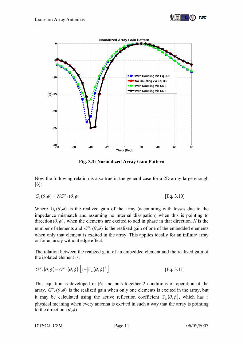
[Eq. 3.9] Therefore, if we know the S parameters of an array of antennas (then we can compute the ARC of every antenna) by using the element pattern of a single isolated antenna and Eq. 3.9 we can compute the actual Array Pattern accounting with the effect of the mutual coupling. In Fig. 3.3 we can see how Eq. 3.9 performs in the case of 2 half wavelength thin dipoles spaced half a wavelength at 9.5 GHz. We believe the small discrepancy between the computation of CST (green-circles line) and the above equation (blue-squares line) for certain angles (-30 to -50 degrees) is due to the pruning that CST applies to the phases during the patter calculation. Furthermore we can appreciate how, by means of using the classical array theory, without accounting for the coupling effect (red-triangle up and black-triangle down lines), the Gain Pattern differs from the real case already in such a simple array.

DTSC-UC3M Page 10 06/02/2007


-80 -60 -40 -20 0 20 40 60 80-30

-25

-20

-15

-10

-5

0

Theta [Deg]

[dB

]

Nomalized Array Gain Pattern

With Coupling via Eq. 3.9No Coupling via Eq. 3.9With Coupling via CSTWith Coupling via CST

Fig. 3.3: Normalized Array Gain Pattern

Now the following relation is also true in the general case for a 2D array large enough [6]:

),(),( φθφθ rm

r NGG = [Eq. 3.10] Where ),( φθrG is the realized gain of the array (accounting with losses due to the impedance mismatch and assuming no internal dissipation) when this is pointing to direction ),( φθ , when the elements are excited to add in phase in that direction. N is the number of elements and is the realized gain of one of the embedded elements when only that element is excited in the array. This applies ideally for an infinite array or for an array without edge effect.

),( φθrmG

The relation between the realized gain of an embedded element and the realized gain of the isolated element is:

( ) ( ) ( )[ ]20 ,1,, φθφθφθ m

mr

m GG Γ−⋅= [Eq. 3.11] This equation is developed in [6] and puts together 2 conditions of operation of the array. is the realized gain when only one elements is excited in the array, but it may be calculated using the active reflection coefficient

),( φθrmG

( )φθ ,mΓ , which has a physical meaning when every antenna is excited in such a way that the array is pointing to the direction ),( φθ .

DTSC-UC3M Page 11 06/02/2007


Therefore, we have seen which parameters affect the final array pattern bandwidth and shape:

• The element type. (The individual pattern is multiplied by the coupling factors)

• The array configuration: triangular, rectangular, circular… This will modify the contributions from the different antennas to the ARC of every element. And this will therefore modify the final array pattern.

• The array spacing, for the same reason than the previous case.

Also the presence of a ground plane or similar modifications of the structure will modify the ARC and the element pattern (modulus and phase of the S parameters) and therefore the array performance. Simulations over the final elements must determine the relation between all these parameters in order to offer the desired characteristics. It is interesting to notice how a good choice of the array configuration and element type may offer unexpected results. Is it possible to get a good combination of the phases (for instance choosing the spacing carefully) in such a way that a certain increment of the array spacing does not necessary affect in a negative way the ARC for the whole spam of angles, even if the absolute value of the S parameters will always decrease as the spacing grows.

DTSC-UC3M Page 12 06/02/2007


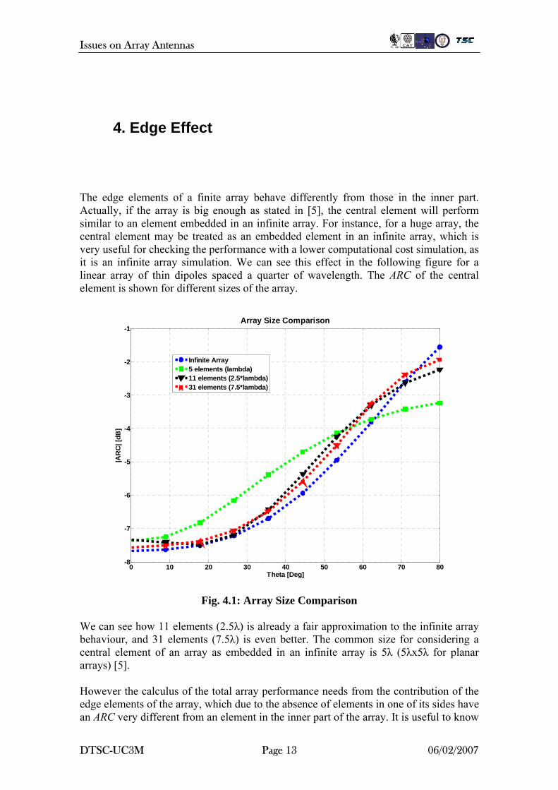
4. Edge Effect The edge elements of a finite array behave differently from those in the inner part. Actually, if the array is big enough as stated in [5], the central element will perform similar to an element embedded in an infinite array. For instance, for a huge array, the central element may be treated as an embedded element in an infinite array, which is very useful for checking the performance with a lower computational cost simulation, as it is an infinite array simulation. We can see this effect in the following figure for a linear array of thin dipoles spaced a quarter of wavelength. The ARC of the central element is shown for different sizes of the array.

0 10 20 30 40 50 60 70 80-8

-7

-6

-5

-4

-3

-2

-1

Theta [Deg]

|AR

C| [

dB]

Array Size Comparison

Infinite Array5 elements (lambda)11 elements (2.5*lambda)31 elements (7.5*lambda)

Fig. 4.1: Array Size Comparison

We can see how 11 elements (2.5λ) is already a fair approximation to the infinite array behaviour, and 31 elements (7.5λ) is even better. The common size for considering a central element of an array as embedded in an infinite array is 5λ (5λx5λ for planar arrays) [5]. However the calculus of the total array performance needs from the contribution of the edge elements of the array, which due to the absence of elements in one of its sides have an ARC very different from an element in the inner part of the array. It is useful to know

DTSC-UC3M Page 13 06/02/2007


how an edge element behave specially in huge arrays, where the central elements may be considered as embedded in an infinite array but we want to know what is the distortion of the coupling in the outer edge of the finite array. In [5] a limit for the edge consideration of an element is given for a special case. In the next section an analytical expression for the ARC of an edge element in a huge array is developed (actually for every element).

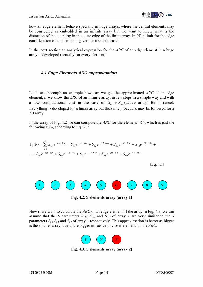
4.1 Edge Elements ARC approximation Let’s see thorough an example how can we get the approximated ARC of an edge element, if we know the ARC of an infinite array, in few steps in a simple way and with a low computational cost in the case of nmmn SS ≠ (active arrays for instance). Everything is developed for a linear array but the same procedure may be followed for a 2D array. In the array of Fig. 4.2 we can compute the ARC for the element “6”, which is just the following sum, according to Eq. 3.1:

ujujujujuj

ujujujujN

n

unjn

eSeSeSeSeS

eSeSeSeSeS

)69(69

)68(68

)67(67

)66(66

)65(65

)64(64

)63(63

)62(62

)61(61

1

)6(66

...

...)(

−−−−−−−−−−

−−−−−−−−

=

−−

+++++

++++==Γ ∑θ

[Eq. 4.1]

7 8 9 1 2 3 4 5 6

Fig. 4.2: 9 elements array (array 1) Now if we want to calculate the ARC of an edge element of the array in Fig. 4.3, we can assume that the S parameters S’33, S’32 and S’31 of array 2 are very similar to the S parameters S66, S65 and S64 of array 1 respectively. This approximation is better as bigger is the smaller array, due to the bigger influence of closer elements in the ARC.

1' 2' 3'

Fig. 4.3: 3 elements array (array 2)

DTSC-UC3M Page 14 06/02/2007


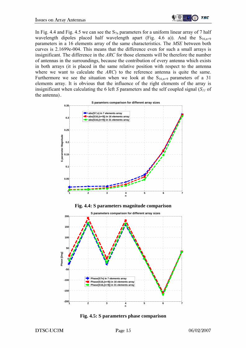
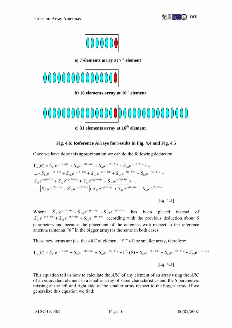
In Fig. 4.4 and Fig. 4.5 we can see the S7n parameters for a uniform linear array of 7 half wavelength dipoles placed half wavelength apart (Fig. 4.6 a)). And the S16,n+9 parameters in a 16 elements array of the same characteristics. The MSE between both curves is 2.1699e-004. This means that the difference even for such a small arrays is insignificant. The difference in the ARC for those elements will be therefore the number of antennas in the surroundings, because the contribution of every antenna which exists in both arrays (it is placed in the same relative position with respect to the antenna where we want to calculate the ARC) to the reference antenna is quite the same. Furthermore we see the situation when we look at the S16,n+9 parameters of a 31 elements array. It is obvious that the influence of the right elements of the array is insignificant when calculating the 6 left S parameters and the self coupled signal (S11 of the antenna).

1 2 3 4 5 6 70

0.05

0.1

0.15

0.2

0.25

0.3

0.35

n

S pa

ram

eter

Mag

nitu

de

S paramters comparison for different array sizes

abs(S7,n) in 7 elements arrayabs(S16,(n+9)) in 16 elements arrayabs(S16,(n+9)) in 31 elements array

Fig. 4.4: S parameters magnitude comparison

1 2 3 4 5 6 7-200

-150

-100

-50

0

50

100

150

200

n

Phas

e [D

eg]

S parameters comparison for different array sizes

Phase(S7n) in 7 elements array Phase(S16,(n+9)) in 16 elements arrayPhase(S16,(n+9)) in 31 elements array

Fig. 4.5: S parameters phase comparison

DTSC-UC3M Page 15 06/02/2007


a) 7 elements array at 7th element

b) 16 elements array at 16th element

c) 31 elements array at 16th element

Fig. 4.6: Reference Arrays for results in Fig. 4.4 and Fig. 4.5

Once we have done this approximation we can do the following deduction:

ujujujujuj

ujujujuj

ujujujujuj

ujujujuj

eSeSeSeSeS

eSeSeSeS

eSeSeSeSeS

eSeSeSeS

)69(69

)68(68

)67(67

)33(33

')32(32

'

)31(31

')63(63

)62(62

)61(61

)69(69

)68(68

)67(67

)66(66

)65(65

)64(64

)63(63

)62(62

)61(616

...

...

...

...)(

−−−−−−−−−−

−−−−−−−−

−−−−−−−−−−

−−−−−−−−

+++++

++++

≈+++++

++++=Γ θ

[Eq. 4.2]

Where has been placed instead of

according with the previous deduction about S parameters and because the placement of the antennas with respect to the reference antenna (antenna “6” in the bigger array) is the same in both cases.

ujujuj eSeSeS )33(33

')32(32

')31(31

' −−−−−− ++ujujuj eSeSeS )66(

66)65(

65)64(

64−−−−−− ++

These new terms are just the ARC of element “3’” of the smaller array, therefore:

ujujujujujuj eSeSeSeSeSeS )69(69

)68(68

)67(673

')63(63

)62(62

)61(616 )()( −−−−−−−−−−−− +++Γ+++≈Γ θθ

[Eq. 4.3]

This equation tell us how to calculate the ARC of any element of an array using the ARC of an equivalent element in a smaller array of same characteristics and the S parameters missing at the left and right side of the smaller array respect to the bigger array. If we generalize this equation we find:

DTSC-UC3M Page 16 06/02/2007

Issues on Array Antennas ∑∑ −

=−

+−−

=−−− +Γ+≈Γ

2/)'(

1 )'(,''2/)'(

1)2/)'((

, )()( NN

kjku

kNNMNNN

kuNNkj

kMM eSeS θθ [Eq. 4.4]

Being N the number of elements of the big array and N’ the number of elements of the small array and the excess of antennas is equally distributed between the right and the left part of the small array (N-N’ must be an even number) for the current formulation. It is also important to notice that this formulation is useful only for edge elements of the small array, but it may be easily modified to apply the same concept for any element in the array. Furthermore if the smaller array is big enough [5], we can apply the approximation of discarding the contribution from those elements in the opposite side of the array respect to the edge element of interest. Finally, if , ∞→N )(θMΓ becomes )(θ∞Γ , the ARC of any element in the infinite array. As more terms we compute in the last sum of Eq. 4.4 a better result may be achieved, implying a trade off between accuracy and computational cost. The ARC of an edge element of a half-infinite array (or equivalently a very big array) may be computed as:

∑ −

=−

+−∞ −Γ≈Γ2/)'(

1)(

)'(,'' )()( KN

iuij

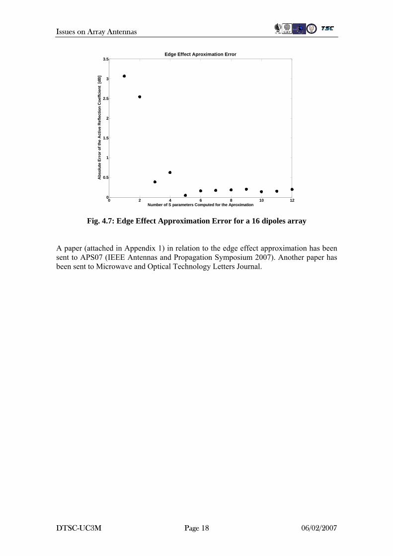
iKNMK eSθθ [Eq. 4.5] In Fig. 4.7, a 16 half wavelength x-axis-oriented thin dipoles array at 9.5 GHz, placed along y-axis and spaced 4λ is used to show the right performance of the method. The absolute error of the ARC absolute value approximation for the outer element is calculated for scanning angles from 0 to 80 degrees in θ direction. The curve decays with an increasing number of terms computed in Eq. 4.5. The residual error of the method must be added to the following result, which in this case is 2 dB. This residual error decreases when the assumptions taken in the method are properly fulfilled, for instance in the case of big arrays [5]. The convergence of the method occurs for 5 terms computed in the approximation.

DTSC-UC3M Page 17 06/02/2007


0 2 4 6 8 10 120

0.5

1

1.5

2

2.5

3

3.5

Number of S parameters Computed for the Aproximation

Abs

olut

e Er

ror o

f the

Act

ive

Ref

lect

ion

Coe

ffcie

nt [

dB]

Edge Effect Aproximation Error

Fig. 4.7: Edge Effect Approximation Error for a 16 dipoles array

A paper (attached in Appendix 1) in relation to the edge effect approximation has been sent to APS07 (IEEE Antennas and Propagation Symposium 2007). Another paper has been sent to Microwave and Optical Technology Letters Journal.

DTSC-UC3M Page 18 06/02/2007


5. Some more issues about Array Antennas

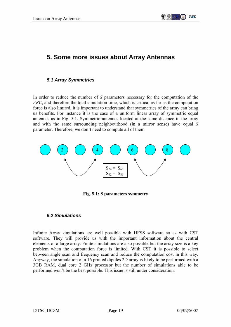
5.1 Array Symmetries In order to reduce the number of S parameters necessary for the computation of the ARC, and therefore the total simulation time, which is critical as far as the computation force is also limited, it is important to understand that symmetries of the array can bring us benefits. For instance it is the case of a uniform linear array of symmetric equal antennas as in Fig. 5.1. Symmetric antennas located at the same distance in the array and with the same surrounding neighbourhood (in a mirror sense) have equal S parameter. Therefore, we don’t need to compute all of them

2 4 6 8

S24 = S68 S42 = S86

Fig. 5.1: S parameters symmetry

5.2 Simulations

Infinite Array simulations are well possible with HFSS software so as with CST software. They will provide us with the important information about the central elements of a large array. Finite simulations are also possible but the array size is a key problem when the computation force is limited. With CST it is possible to select between angle scan and frequency scan and reduce the computation cost in this way. Anyway, the simulation of a 16 printed dipoles 2D array is likely to be performed with a 3GB RAM, dual core 2 GHz processor but the number of simulations able to be performed won’t be the best possible. This issue is still under consideration.

DTSC-UC3M Page 19 06/02/2007


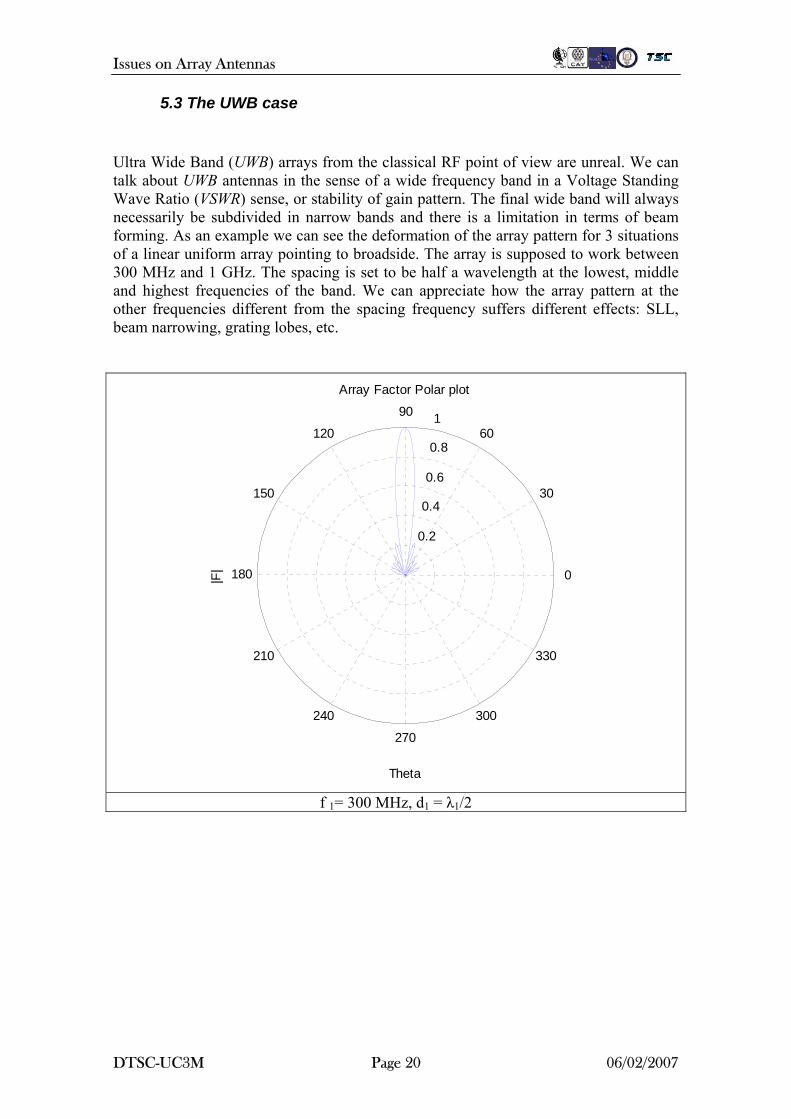
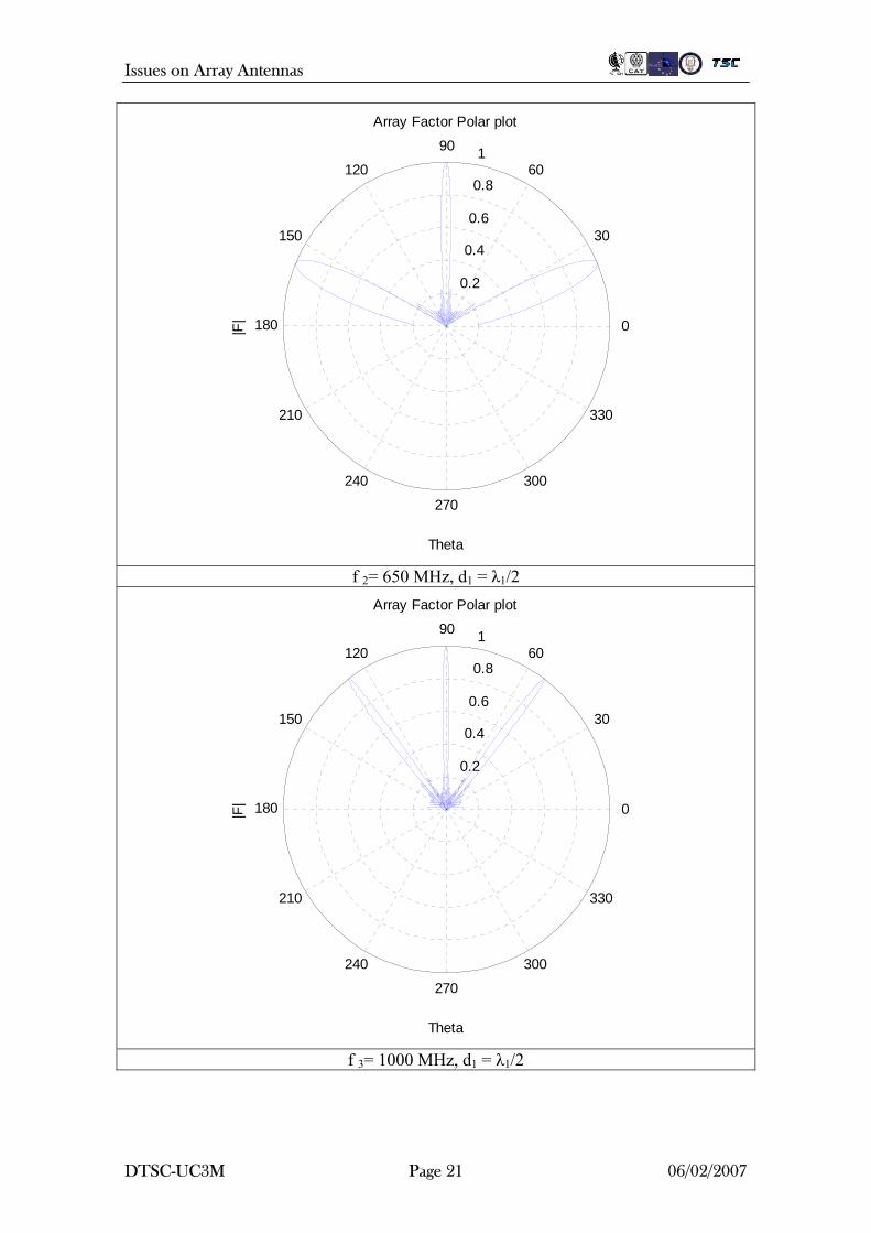
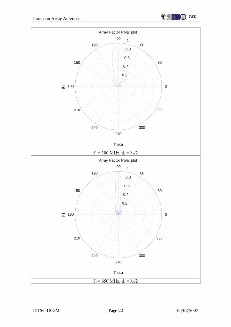
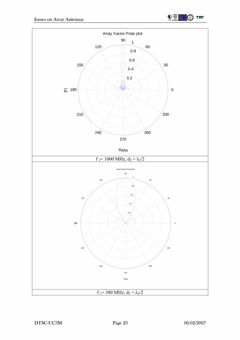
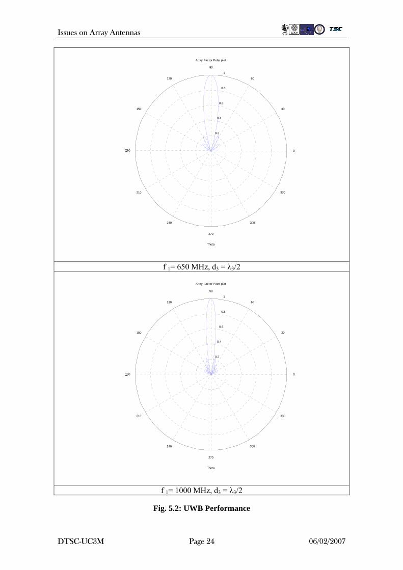
5.3 The UWB case Ultra Wide Band (UWB) arrays from the classical RF point of view are unreal. We can talk about UWB antennas in the sense of a wide frequency band in a Voltage Standing Wave Ratio (VSWR) sense, or stability of gain pattern. The final wide band will always necessarily be subdivided in narrow bands and there is a limitation in terms of beam forming. As an example we can see the deformation of the array pattern for 3 situations of a linear uniform array pointing to broadside. The array is supposed to work between 300 MHz and 1 GHz. The spacing is set to be half a wavelength at the lowest, middle and highest frequencies of the band. We can appreciate how the array pattern at the other frequencies different from the spacing frequency suffers different effects: SLL, beam narrowing, grating lobes, etc.

0.2

0.4

0.6

0.8

1

30

210

60

240

90

270

120

300

150

330

180 0

Array Factor Polar plot

Theta

|F|

f 1= 300 MHz, d1 = λ1/2

DTSC-UC3M Page 20 06/02/2007


0.2

0.4

0.6

0.8

1

30

210

60

240

90

270

120

300

150

330

180 0


Theta

|F|

f 2= 650 MHz, d1 = λ1/2

0.2

0.4

0.6

0.8

1

30

210

60

240

90

270

120

300

150

330

180 0


Theta

|F|

f 3= 1000 MHz, d1 = λ1/2

DTSC-UC3M Page 21 06/02/2007


0.2

0.4

0.6

0.8

1

30

210

60

240

90

270

120

300

150

330

180 0


Theta

|F|

f 1= 300 MHz, d2 = λ2/2

0.2

0.4

0.6

0.8

1

30

210

60

240

90

270

120

300

150

330

180 0


Theta

|F|

f 2= 650 MHz, d2 = λ2/2

DTSC-UC3M Page 22 06/02/2007


0.2

0.4

0.6

0.8

1

30

210

60

240

90

270

120

300

150

330

180 0


Theta

|F|

f 3= 1000 MHz, d2 = λ2/2

0.2

0.4

0.6

0.8

1

30

210

60

240

90

270

120

300

150

330

180 0


Theta

|F|

f 1= 300 MHz, d3 = λ3/2

DTSC-UC3M Page 23 06/02/2007


0.2

0.4

0.6

0.8

1

30

210

60

240

90

270

120

300

150

330

180 0


Theta

|F|

f 1= 650 MHz, d3 = λ3/2

0.2

0.4

0.6

0.8

1

30

210

60

240

90

270

120

300

150

330

180 0


Theta

|F|

f 1= 1000 MHz, d3 = λ3/2

Fig. 5.2: UWB Performance

DTSC-UC3M Page 24 06/02/2007


6. Future Lines The future lines of work will cover the following aspects. Some of the tasks are already being performed but the results are still not remarkable:

• Use of Genetic Algorithms to find an optimum space interleaving, element shape and array configuration in terms of ARC. So far the results point to the use of a uniform interleaving.

• Study of the array polarization and phasing together: How does the element

type, spacing and array configuration affect. • First simulations of real elements (mainly wide band printed dipoles) in finite

arrays. So far the results show a high computational cost for the whole finite array.

• Array configuration: triangular, circular, square, etc.

DTSC-UC3M Page 25 06/02/2007


7. Conclusions

This report summarizes a close study about the important parameters of finite and infinite phased antenna arrays: meaning of the parameters, effects, causes, computation…. Once we know the cause-effect relations and how to compute them, this knowledge will allow us to properly design the radiating elements, so as the array configuration: elements distribution, spacing, etc. in order to get the desired characteristics for the subset of antennas which will compose the final sub array: beamwidth, frequency bandwidth, scan angles, etc. The text is mainly composed of:

• Review of classical array theory.

• Presentation of the key parameter: Active Reflection Coefficient and its relation to the array pattern. Mutual Coupling. Which parameters need to be considered.

• Study of the size of the array: Edge Effect.

• Some more issues: Simulations and other considerations.

DTSC-UC3M Page 26 06/02/2007


8. References [1] Warren L. Stutzman and Gary A. Thiele, Antenna Theory and esign, 2nd ed., John Wiley & Sons, 1998. [2] M. I. Skolnik, Ed., Radar Handbook, 2nd ed. New York: McGraw-Hill, 1991. [3] D. M. Pozar, “A relation between the active input impedance and the active element pattern of a phased array,” IEEE Trans. Antennas Propagation, vol. 51, no. 9, pp. 2486–2489, Sep. 2003. [4] D. M. Pozar, “The active element pattern,” IEEE Trans. Antennas Propagat., vol. 42, no. 8, pp. 1176–1178, 1994. [5] H. Holter and H. Steyskal, “On the size requirement for finite phased array models,” IEEE Trans. Antennas Propagation, vol. 50, pp. 836–840, June 2002. [6] P. W. Hannan, “The element-gain paradox for a phased array antenna,” IEEE Trans. Antennas and Propagation, vol. AP-12,. pp. 423-433, July 1964.

DTSC-UC3M Page 27 06/02/2007


Appendices

Appendix 1: Mutual Coupling Edge Effect Approximation for Phased-Array Antennas

DTSC-UC3M Page 28 06/02/2007

Mutual Coupling Edge Effect Approximation for Phased-Array Antennas

E. De Lera*(1)(2), E. Garcia (2) (1) Yebes Astronomical Center, National Astronomical Observatory 19080,

Apdo. 148, Yebes, Guadalajara, Spain (2) Signal Theory and Communications Dpt. Carlos III University of Madrid

Avda. Universidad 30, 28911, Leganes, Madrid, Spain

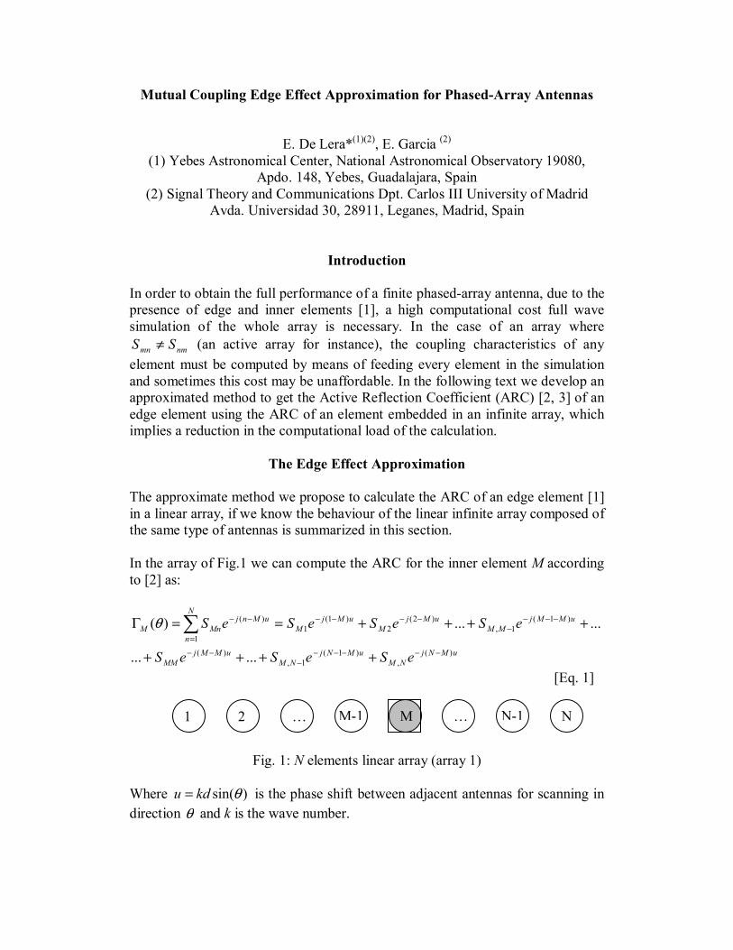
Introduction

In order to obtain the full performance of a finite phased-array antenna, due to the presence of edge and inner elements [1], a high computational cost full wave simulation of the whole array is necessary. In the case of an array where

nmmn SS ≠ (an active array for instance), the coupling characteristics of any element must be computed by means of feeding every element in the simulation and sometimes this cost may be unaffordable. In the following text we develop an approximated method to get the Active Reflection Coefficient (ARC) [2, 3] of an edge element using the ARC of an element embedded in an infinite array, which implies a reduction in the computational load of the calculation.

The Edge Effect Approximation The approximate method we propose to calculate the ARC of an edge element [1] in a linear array, if we know the behaviour of the linear infinite array composed of the same type of antennas is summarized in this section. In the array of Fig.1 we can compute the ARC for the inner element M according to [2] as:

uMNjNM

uMNjNM

uMMjMM

uMMjMM

uMjM

uMjM

N

n

uMnjMnM

eSeSeS

eSeSeSeS

)(,

)1(1,

)(

)1(1,

)2(2

)1(1

1

)(

......

......)(

−−−−−−

−−

−−−−

−−−−

=

−−

++++

++++==Γ ∑θ

[Eq. 1]

Fig. 1: N elements linear array (array 1)

Where )sin(θkdu = is the phase shift between adjacent antennas for scanning in direction θ and k is the wave number.

1 2 … M … N N-1M-1

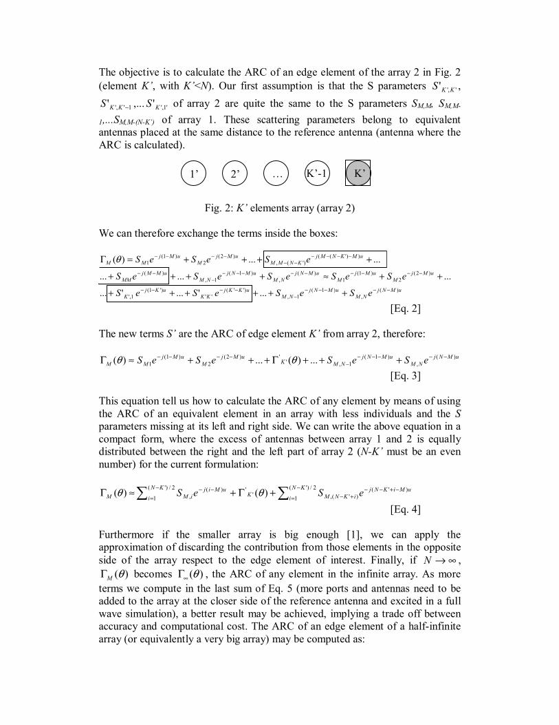
The objective is to calculate the ARC of an edge element of the array 2 in Fig. 2 (element K’, with K’<N). Our first assumption is that the S parameters ','' KKS ,

1','' −KKS ,... '1,''KS of array 2 are quite the same to the S parameters SM,M, SM,M-

1,...SM,M-(N-K’) of array 1. These scattering parameters belong to equivalent antennas placed at the same distance to the reference antenna (antenna where the ARC is calculated).

Fig. 2: K’ elements array (array 2) We can therefore exchange the terms inside the boxes:

uMNjNM

uMNjNM

uKKjKK

uKjK

uMjM

uMjM

uMNjNM

uMNjNM

uMMjMM

uMKNMjKNMM

uMjM

uMjMM

eSeSeSeS

eSeSeSeSeS

eSeSeS

)(,

)1(1,

)''(''

)'1(1,'

)2(2

)1(1

)(,

)1(1,

)(

))'(()'(,

)2(2

)1(1

...'...'...

.........

......)(

−−−−−−

−−−−

−−−−−−−−−−

−−

−−−−−−

−−−−

++++++

++≈++++

++++=Γ θ

[Eq. 2] The new terms S’ are the ARC of edge element K’ from array 2, therefore:

uMNjNM

uMNjNMK

uMjM

uMjMM eSeSeSeS )(

,)1(

1,'')2(

2)1(

1 ...)(...)( −−−−−−

−−−− +++Γ+++≈Γ θθ [Eq. 3]

This equation tell us how to calculate the ARC of any element by means of using the ARC of an equivalent element in an array with less individuals and the S parameters missing at its left and right side. We can write the above equation in a compact form, where the excess of antennas between array 1 and 2 is equally distributed between the right and the left part of array 2 (N-K’ must be an even number) for the current formulation:

∑∑ −

=−+−−

+−−

=−− +Γ+≈Γ 2/)'(

1)'(

)'(,''2/)'(

1)(

, )()( KN

iuMiKNj

iKNMKKN

iuMij

iMM eSeS θθ [Eq. 4]

Furthermore if the smaller array is big enough [1], we can apply the approximation of discarding the contribution from those elements in the opposite side of the array respect to the edge element of interest. Finally, if ∞→N ,

)(θMΓ becomes )(θ∞Γ , the ARC of any element in the infinite array. As more terms we compute in the last sum of Eq. 5 (more ports and antennas need to be added to the array at the closer side of the reference antenna and excited in a full wave simulation), a better result may be achieved, implying a trade off between accuracy and computational cost. The ARC of an edge element of a half-infinite array (or equivalently a very big array) may be computed as:

… K’K’-11’ 2’

∑ −

=−

+−∞ −Γ≈Γ 2/)'(

1)(

)'(,'' )()( KN

iuij

iKNMK eSθθ [Eq. 5] The same procedure may be followed for a 2D array. The performance of the method is demonstrated in the next section.

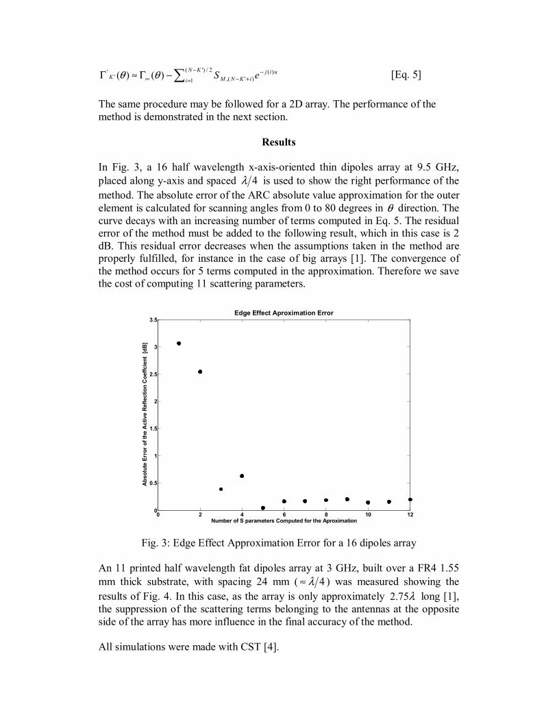
Results

In Fig. 3, a 16 half wavelength x-axis-oriented thin dipoles array at 9.5 GHz, placed along y-axis and spaced 4λ is used to show the right performance of the method. The absolute error of the ARC absolute value approximation for the outer element is calculated for scanning angles from 0 to 80 degrees in θ direction. The curve decays with an increasing number of terms computed in Eq. 5. The residual error of the method must be added to the following result, which in this case is 2 dB. This residual error decreases when the assumptions taken in the method are properly fulfilled, for instance in the case of big arrays [1]. The convergence of the method occurs for 5 terms computed in the approximation. Therefore we save the cost of computing 11 scattering parameters.

0 2 4 6 8 10 120

0.5

1

1.5

2

2.5

3

3.5

Number of S parameters Computed for the Aproximation

Abs

olut

e Er

ror

of th

e A

ctiv

e R

efle

ctio

n C

oeffc

ient

[dB

]

Edge Effect Aproximation Error

Fig. 3: Edge Effect Approximation Error for a 16 dipoles array

An 11 printed half wavelength fat dipoles array at 3 GHz, built over a FR4 1.55 mm thick substrate, with spacing 24 mm ( 4λ≈ ) was measured showing the results of Fig. 4. In this case, as the array is only approximately λ75.2 long [1], the suppression of the scattering terms belonging to the antennas at the opposite side of the array has more influence in the final accuracy of the method. All simulations were made with CST [4].

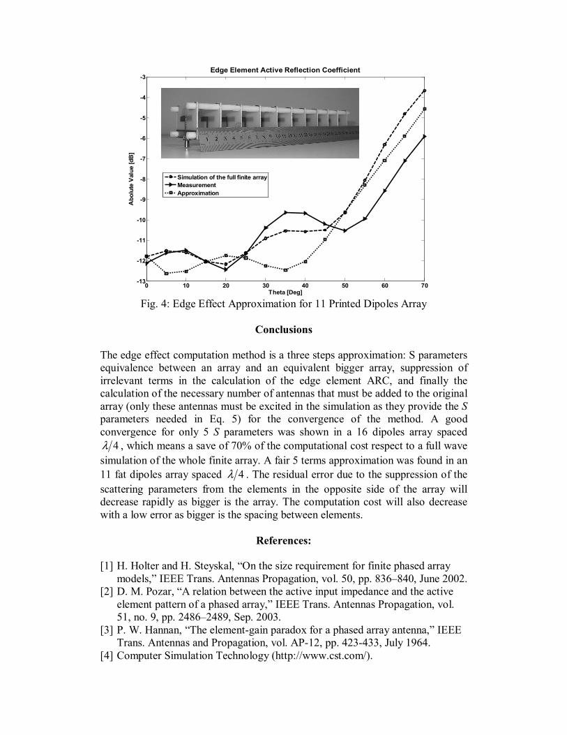
Fig. 4: Edge Effect Approximation for 11 Printed Dipoles Array

Conclusions

The edge effect computation method is a three steps approximation: S parameters equivalence between an array and an equivalent bigger array, suppression of irrelevant terms in the calculation of the edge element ARC, and finally the calculation of the necessary number of antennas that must be added to the original array (only these antennas must be excited in the simulation as they provide the S parameters needed in Eq. 5) for the convergence of the method. A good convergence for only 5 S parameters was shown in a 16 dipoles array spaced

4λ , which means a save of 70% of the computational cost respect to a full wave simulation of the whole finite array. A fair 5 terms approximation was found in an 11 fat dipoles array spaced 4λ . The residual error due to the suppression of the scattering parameters from the elements in the opposite side of the array will decrease rapidly as bigger is the array. The computation cost will also decrease with a low error as bigger is the spacing between elements.

References: [1] H. Holter and H. Steyskal, “On the size requirement for finite phased array

models,” IEEE Trans. Antennas Propagation, vol. 50, pp. 836–840, June 2002. [2] D. M. Pozar, “A relation between the active input impedance and the active

element pattern of a phased array,” IEEE Trans. Antennas Propagation, vol. 51, no. 9, pp. 2486–2489, Sep. 2003.

[3] P. W. Hannan, “The element-gain paradox for a phased array antenna,” IEEE Trans. Antennas and Propagation, vol. AP-12, pp. 423-433, July 1964.

[4] Computer Simulation Technology (http://www.cst.com/).

0 10 20 30 40 50 60 70-13

-12

-11

-10

-9

-8

-7

-6

-5

-4

-3

Theta [Deg]

Abo

lute

Val

ue [d

B]

Edge Element Active Reflection Coefficient

Simulation of the full finite arrayMeasurementApproximation

Documents

Phased Array Antennas - Real Observatorio · DTSC-UC3M Page 2 06/02/2007 . Issues on Array Antennas 1. Introduction The very first step when we seek for the understanding of phased