Phased Array Simulations using Finite Integration Technique

Franz Hirtenfelder CST GmbH, Bad Nauheimerstr. 19, 64289 Darmstadt, Germany

Phone : +49 6151 73030, Fax : +49 6151 730310 Web: http://www.cst.com

email: franz.hirtenfelder@cst.com

Jérôme Mollet CST France, 63-65 rue du Fort, 92320 Châtillon, France

Phone : +33-1-46 44 90 64, Fax : +33-1-46 48 61 74 Web : http://www.cst.com

email : jerome.mollet@cst.com

Abstract Phased array antennas are planar double-periodic structures that find many applications in electronic systems. One of the methods of analyzing phased arrays is to assume that the array is infinite. The infinite array idealization for antenna arrays is a powerful analysis tool. Although it neglects edge effects, it provides the essential design parameters for large antenna arrays. The application of the finite integration technique (FIT) to infinite array analysis offers many advantages: 1) complicated geometries and materials can be analyzed, where no analytic Green’s functions for a method of moment technique are available, 2) the FIT is a general tool that avoids the need to develop new codes for new radiators, 3) since only one unit cell with phase shift walls is analyzed, the model size fits the computational capabilities of present PCs and reduces drastically runtimes. This paper describes the application of a single periodic slotted waveguide phased-array antenna fed by a coaxial line. The scan is performed in both, the E- and H-Plane. The absorbing boundaries are placed in some distance away from the aperture and absorb the generated plane waves of the periodic structure. Complex periodic boundary conditions sustain the propagation of the plane waves at the model’s side walls. The results of the farfield scan at zero degree phase shift for both, the complete model and the unit cell model are in very good agreement with measurements.

1 Introduction

The analysis of phased-array antennas has been an important research and design area for the last couple of decades. Till now the main numerical tool for analyzing phased-array radiating elements was the MOM [1]. It deserved the development of specific codes for the different types of elements used in phased arrays, dipoles, open waveguides, notches, slots, micro-strips, etc. All of these codes were developed by electronic system companies with the help of intensive academic research. As phased array antennas progresses the geometrical complexity of the design, the use of new dielectric materials and the demand for monolithic designs all raise the need for a general tool that would be able to analyze any phased-array radiating element.

2 Numerical techniques

In this section, the numerical techniques employed for the 3D field simulation and for the subsequent determination of the far field and S-parameters are briefly described.

2.1 The Finite Integration Technique

The numerical method used for the field simulation is the Finite Integration Technique (FIT), first proposed by Weiland in 1977 [2]. FIT generates exact algebraic analogues to Maxwell’s equations, which guarantee that the physical properties of fields are maintained in the discrete space, and lead to a unique solution. Maxwell's equations and the related material equations are transformed from the continuous to the discrete space by allocating electric voltages on the edges of a grid G and magnetic voltages on the edges of a dual grid G

~ . The allocation of the voltage and flux components on the grid can be seen in Fig. 1. The use of integral degrees of freedom, i.e. voltages and fluxes, instead of field components (such as used in FDTD) allows not only a very elegant way of writing the matrix equations (1-4), but also has important algorithmic-theoretical and numerical consequences [3]. The discrete equivalent of Maxwell's equations, the so-called Maxwell’s Grid Equations are shown in Eqs. (1)-(4). This description is still an exact representation and does not contain any approximation errors.

beC���

dtd−= jdhC

�����

+=dtd~

(1, 2)

0bS =��

qdS =��~

(3, 4)

In these equations e� and h�

denote the electric and magnetic voltages along primary and dual edges, respectively.

Fig. 1: Allocation of the voltage and flux components

in the mesh. Fig. 2: The leap-frog scheme.

The symbols d��

, b��

and j��

are the electric, magnetic, and current-density fluxes across primary and dual grid faces. The

topological matrices C , C~

, S and S~ represent the discrete equivalents of the curl- and the div-operators, with the tilde

indicating the dual grid. The discrete analogues of material property relations express the coupling between voltages and fluxes, through the material matrices εM , 1−µM and σM .

eMd �

���

= bMh 1�

���

−= AjeMj���

��

+= σ (5, 6, 7)

These matrices have diagonal form and contain the unavoidable approximations of any numerical procedure. The FIT can be applied to different frequency ranges, from DC to THz. On Cartesian grids, the time-domain FIT can be rewritten to yield the FDTD scheme. However, whereas the classical FDTD has the disadvantage of the staircase approximation of complex boundaries, the Perfect Boundary Approximation� (PBA) [4] technique applied in conjunction with FIT maintains all the advantages of the structured Cartesian grids, while allowing an accurate modeling of curved boundaries. The boundary of the calculation domain is assumed to be ideal electric, ideal magnetic or ‘open’. The perfectly matched layer (PML) [5] is used in the case of open boundaries.

2.2 Time Domain Simulation

The time-domain FIT is the most efficient scheme for many RF-applications. For the discretization of the time derivative, the well-known explicit leap-frog algorithm is used. It is very memory-efficient and has the advantage that the calculation of the unknowns at each time step only requires one matrix-vector multiplication (linear complexity). This scheme is illustrated in Fig 2. FIT in time domain is therewith a generalization of the FDTD method. The excitation signal for the time domain calculation can be fed in the structure on any desired path of edges in the primary grid. This path is referred to as discrete port. More complex waveguide structures are excited with a so-called waveguide port. For the computation of S-parameters, one or several discrete or waveguide ports are defined in the computational domain or at its boundary, respectively. To obtain a full S-parameter matrix, all ports are excited successively with an appropriate time-domain pulse, and the output (reflected or transmitted) signals at all further ports are recorded. To calculate the S-parameters in a wide range of frequencies, a broadband input signal is chosen, typically a Gauss modulated sine function. All input and output signals resulting from the time domain simulation are then transformed into the frequency domain by application of a Discrete Fourier Transform (DFT) algorithm. Finally, the S-parameters are obtained as the ratio of these frequency domain representations of the direct incident and inverse wave components.

2.3 Frequency Domain

FIT is not restricted to Time Domain simulations; it can also be formulated in the Frequency Domain, where the treatment of periodic structures particularly important in Radar technology, is very handy. In the commercial software CST MICROWAVE STUDIO® a periodic (Floquet Mode) boundary port mode solver is implemented that delivers highest accuracy for wide radiation angles, especially for phased array calculations. The Floquet Mode solver allows to separate the grating lobe from the main radiating mode, and thus allows to specify the power transmission factor for the principal mode directly. Since the plane wave is also a solution of the periodic boundary port, the illumination of Frequency Selective Surfaces (FSS) under arbitrary angle can be easily done. Maxwell’s Grid Equations in time harmonics, driven by imprinted (displacement) currents can be expressed as following:

hMjbjeC����

µωω −=−= Ii eMjeMjjjdjhC ���������

εε ωωω +=++=~ (8,9)

0=bS��

0~ =dS��

(10,11) finally leading to the curl-curl equation which has to be solved by e.g. Modified-Krylov-Subspace Method:

IeMeMeCMC ���

εεν ωω 22~ =− (12)

The depending degrees of freedom of the electric fields E are linked to the independent ones obeying the equation

indepj

dep EeE .φ= (13)

and are eliminated from the equation system. The relation between the electrical phase shift yx ξξ , and the scan direction

is given by ssxx kd ϕθξ cossin= ssyy kd ϕθξ cossin= (14,15)

3 A practical Example

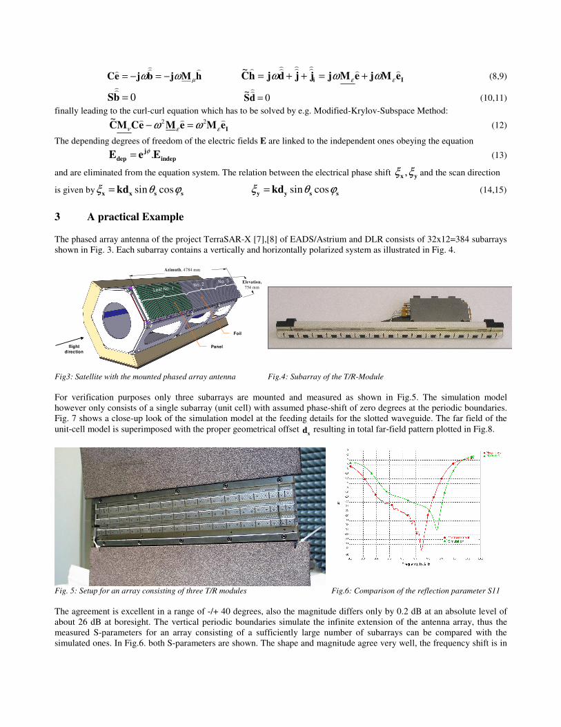
The phased array antenna of the project TerraSAR-X [7],[8] of EADS/Astrium and DLR consists of 32x12=384 subarrays shown in Fig. 3. Each subarray contains a vertically and horizontally polarized system as illustrated in Fig. 4.

Leaf No. 1No. 2 No. 3

Azimuth, 4784 mm

Elevation,754 mm

Foil

Panelflightdirection

Fig3: Satellite with the mounted phased array antenna Fig.4: Subarray of the T/R-Module For verification purposes only three subarrays are mounted and measured as shown in Fig.5. The simulation model however only consists of a single subarray (unit cell) with assumed phase-shift of zero degrees at the periodic boundaries. Fig. 7 shows a close-up look of the simulation model at the feeding details for the slotted waveguide. The far field of the unit-cell model is superimposed with the proper geometrical offset xd resulting in total far-field pattern plotted in Fig.8.

Fig. 5: Setup for an array consisting of three T/R modules Fig.6: Comparison of the reflection parameter S11 The agreement is excellent in a range of -/+ 40 degrees, also the magnitude differs only by 0.2 dB at an absolute level of about 26 dB at boresight. The vertical periodic boundaries simulate the infinite extension of the antenna array, thus the measured S-parameters for an array consisting of a sufficiently large number of subarrays can be compared with the simulated ones. In Fig.6. both S-parameters are shown. The shape and magnitude agree very well, the frequency shift is in

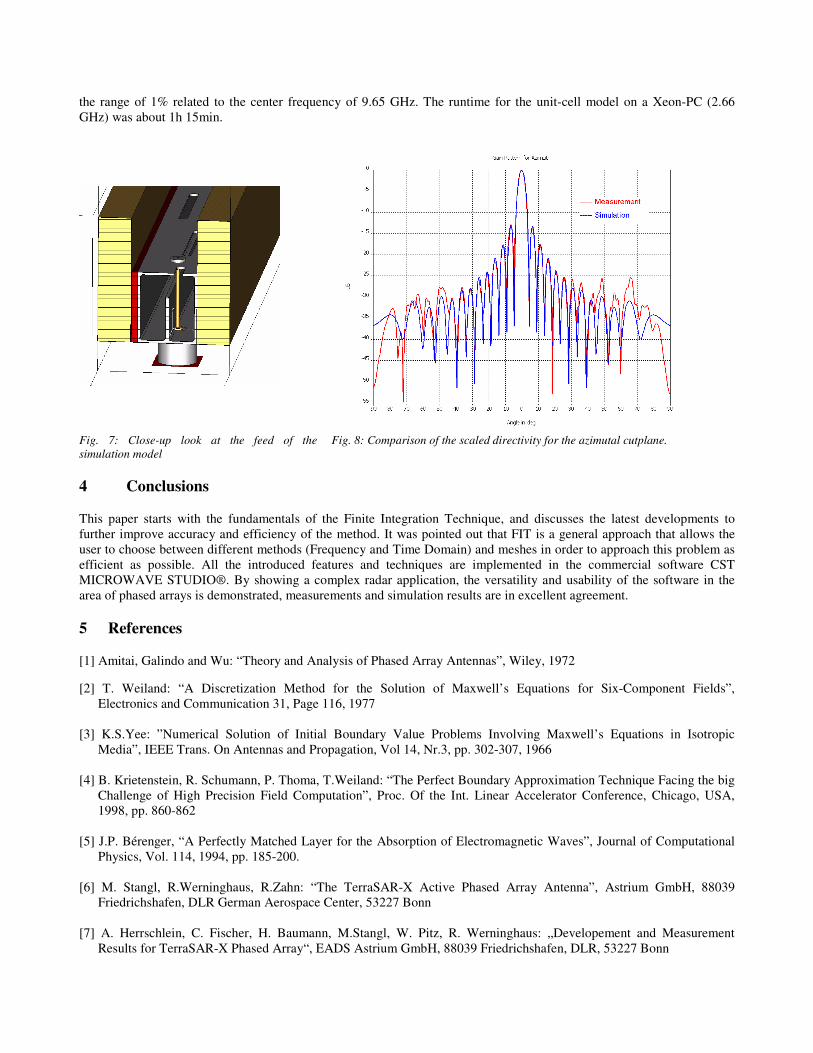
the range of 1% related to the center frequency of 9.65 GHz. The runtime for the unit-cell model on a Xeon-PC (2.66 GHz) was about 1h 15min.

Fig. 7: Close-up look at the feed of the simulation model

Fig. 8: Comparison of the scaled directivity for the azimutal cutplane.

4 Conclusions

This paper starts with the fundamentals of the Finite Integration Technique, and discusses the latest developments to further improve accuracy and efficiency of the method. It was pointed out that FIT is a general approach that allows the user to choose between different methods (Frequency and Time Domain) and meshes in order to approach this problem as efficient as possible. All the introduced features and techniques are implemented in the commercial software CST MICROWAVE STUDIO®. By showing a complex radar application, the versatility and usability of the software in the area of phased arrays is demonstrated, measurements and simulation results are in excellent agreement.

5 References

[1] Amitai, Galindo and Wu: “Theory and Analysis of Phased Array Antennas”, Wiley, 1972 [2] T. Weiland: “A Discretization Method for the Solution of Maxwell’s Equations for Six-Component Fields”,

Electronics and Communication 31, Page 116, 1977

[3] K.S.Yee: ”Numerical Solution of Initial Boundary Value Problems Involving Maxwell’s Equations in Isotropic Media”, IEEE Trans. On Antennas and Propagation, Vol 14, Nr.3, pp. 302-307, 1966

[4] B. Krietenstein, R. Schumann, P. Thoma, T.Weiland: “The Perfect Boundary Approximation Technique Facing the big Challenge of High Precision Field Computation”, Proc. Of the Int. Linear Accelerator Conference, Chicago, USA, 1998, pp. 860-862

[5] J.P. Bérenger, “A Perfectly Matched Layer for the Absorption of Electromagnetic Waves”, Journal of Computational

Physics, Vol. 114, 1994, pp. 185-200. [6] M. Stangl, R.Werninghaus, R.Zahn: “The TerraSAR-X Active Phased Array Antenna”, Astrium GmbH, 88039

Friedrichshafen, DLR German Aerospace Center, 53227 Bonn

[7] A. Herrschlein, C. Fischer, H. Baumann, M.Stangl, W. Pitz, R. Werninghaus: „Developement and Measurement Results for TerraSAR-X Phased Array“, EADS Astrium GmbH, 88039 Friedrichshafen, DLR, 53227 Bonn