Embed Size (px)
Citation preview
PHYSICAL PROPERTIES OF THE LUNAR SURFACE W. David Carrier III, Gary R. Olhoeft, and Wendell Mendell
This chapter discusses the physical properties of the lunar surface, determined at depths varying from a few micrometers to a few tens of meters. The properties considered include geotechnical properties (those properties of a planetary surface needed to evaluate engineering problems, including the mechanical properties of soil and rock), electrical and electromagnetic properties, and the reflection and emission of radiation.
The lunar surface material (regolith or “lunar soil”) is a complex mixture of five basic particle types: crystalline rock fragments, mineral fragments, breccias, agglutinates, and glasses. The relative proportion of each particle type varies from place to place and is dependent on the mineralogy of the source rocks and the geologic processes that the rocks have undergone (see Chapters 4 and 7 for more details).
The lunar regolith is distinctly different from terrestrial materials. For one thing, its mineral composition is limited. Fewer than a hundred minerals have been found on the Moon, compared to several thousand on Earth (see Chapter 5). Furthermore, continuous meteoroid impact has converted the lunar surface materials into a well-graded silty sand that has reached a “steady state” in thickness, particle size distribution, and other properties at most locations on the Moon. Hence, the limited particle types and sizes, the absence of a lunar atmosphere, and the lack of water and organic material in the regolith constrain the physical properties of the lunar surface material to relatively narrow, well-defined ranges. The primary factors that affect the physical properties are bulk density, relative density, and temperature.
The physical properties of lunar soils and rocks have been measured in situ by robots and astronauts, in the laboratory on returned samples, and by remote sensing from the Earth’s surface and from lunar orbit. The results of these measurements are presented in the following sections.
9.1. GEOTECHNICAL PROPERTIES
“I’m at the foot of the ladder. The LM [Lunar Module] footpads are only depressed in the surface about 1 or 2 inches, although the surface appears to be very, very fine-grained, as you get close to it, it’s almost like a powder; down there, it’s very fine ... I’m going to step off the LM now. That’s one small step for (a) man. One giant leap for mankind. As the—The surface is fine and powdery. I can—I can pick it up loosely with my toe. It does adhere in fine layers like powdered charcoal to the sole and sides of my boots. I only go in a small fraction of an inch. Maybe an eighth of an inch, but I can see the footprints of my boots and the treads in the fine sandy particles.”
Neil A. Armstrong Tranquillity Base (Apollo 11),
July 20, 1969
Prior to the Luna, Surveyor, and Apollo soft landings on the Moon, various theories had been proposed regarding the nature of the lunar surface. One theory was that the lunar craters were volcanic in origin and that the surface was mostly lava and hence very hard. The other popular theory was that the craters had been formed by meteoroid impact
475
9
476 Lunar Sourcebook
and that the surface was a regolith or soil with diverse particle sizes. In short, the lunar surface might be either very hard or very soft. The “hard soil” advocates believed that the ultrahigh vacuum conditions on the Moon would produce “cold welding” between the soil particles. This phenomenon is known to occur if two carefully cleaned surfaces (e.g., of aluminum) are brought together in a vacuum. The lack of water and organic molecules in the lunar vacuum would allow the surfaces to bond atomically or weld. Experiments had also shown that the mineral mica could be cleaved and pressed back together in a vacuum. Thus, the lunar surface was thought to be porous and yet rock-hard, like pumice. At the other extreme, it was believed that the combination of low gravity, vacuum, and electrostatic charges on the soil particles would produce a “fairy-castle” structure, with a consistency similar to sifted flour.
Because of the long lead time required, the design of the Apollo Lunar Module (LM) landing gear had to be completed in the mid-1960s, before there were any direct tactile data available about the lunar surface. Because of the different theories that were being hotly debated at that time, the engineers chose a landing gear that could accommodate a wide range of conditions. To accommodate the “soft” extreme of possible lunar surface properties, the LM landing pad was sized so that it could sink as much as 60 cm into the soil and would have a bearing pressure on the Moon of only approximately 4.6 kPa. This value is only about one-fifth of the stress that a typical person exerts when standing on one foot on Earth. To accommodate the “hard” extreme, a shock absorber system was built into the LM landing struts; this system would allow a safe landing on concrete at a vertical velocity of up to 3 m/sec, which is equivalent to free-fall from a height of 2.9 m in lunar gravity. This shock absorber consisted of a honeycomb material that would crush as the landing struts were forced into it during touchdown, thereby dissipating the energy of impact. Unlike the normal hydraulic shock absorber system in an aircraft, the landing gear on the LM only had to work once and could therefore use the crushable design, which was both simpler and lighter.
The landing pads of the pre-Apollo Surveyor spacecraft were sized for a bearing pressure of 2.2 kPa, and when these unmanned probes were successfully soft-landed on the Moon during 1966-1968, the design of the Apollo LM pads was confirmed as conservative. In spite of this evidence, some scientists were still concerned about the bearing capacity of the lunar surface and recommended that the astronauts have snowshoes and that the LM be equipped with a long radio antenna
in case it disappeared into the soft dust at touch-down (Cooper, 1969, 1970). Just a few months before the flight of Apollo 11, it was seriously suggested that, when Astronaut Armstrong took his first steps on the lunar surface, the soil would jump onto his spacesuit because of the electrostatic attraction. The resulting coating of soil covering his suit was expected to be so thick that he would not be able to see and might not be able to move. Then, if he were able to stagger back into the LM, there was concern that the highly reduced soil would burst into flames when the cabin was repressurized with pure oxygen. Even after several successful Apollo missions to the Moon, some scientists were still convinced that the lunar soil was like fresh snow and that an astronaut could push a rod into it to almost any desired depth.
We now know that the lunar surface is neither so soft, nor so hard, as was once imagined. We also know that the astronauts can land a spacecraft far more gently than the designed 3 m/sec. In fact, the landing struts were stroked only slightly on all of the six Apollo landings. Furthermore, we know that the ranges of geotechnical properties of lunar materials are less than those that occur in surficial materials on Earth. This is because of the following factors:
1. The familiar terrestrial geologic processes of chemical weathering, running water, wind, and glaciation are absent on the Moon. These processes tend to produce well-sorted sediments with uniform grain sizes. The primary lunar soil-forming process is meteoroid impact, which produces a heterogeneous and well-graded (poorly-sorted) soil.
2. The three main constituents most likely to produce unusual or “problem” soils on Earth are absent on the Moon; there is no water, and there are no clay minerals or organic materials.
3. As discussed in Chapters 5 and 7, the variety of minerals in lunar soil is much less than that found on Earth. In fact, many soil particles are simply fragments of rocks, minerals, and glass stuck together with glass (agglutinates).
As a result, the geotechnical properties of lunar soil tend to fall in a fairly narrow range, and the most significant variable is the relative density, defined in section 9.1.5. To a certain extent, relative density also controls the other physical properties discussed in this chapter.
To set the stage for discussion of the effects of relative density, other properties will be described first: particle size distribution, particle shapes, specific gravity, bulk density, and porosity. Relative density will then be described. After that, the influence of these properties on compressibility, shear strength, permeability, bearing capacity, slope stability, and trafficability will be considered.
Physical Properties of the Lunar Surface 477
9.1.1. Particle Size Distribution
The particle size distribution in an unconsolidated material, such as lunar soil, is a variable that controls to various degrees the strength and compressibility of the material, as well as its optical, thermal, and seismic properties (Carrier, 1973). Particle size analyses of terrestrial clastic sediments (sediments that are composed of broken fragments from preexisting rocks and minerals that have been transported some distance, e.g., sandstone) are the basic descriptive element for any clastic material (Tucker, 1981) and also provide information on their origin and the depositional processes affecting them. The phi (φ) scale used commonly for measuring particle size is not linear but is a logarithmic transformation of a geometric scale such that φ= -log2d, where d is the particle diameter in millimeters (Folk, 1968; Pettijohn et al., 1973).
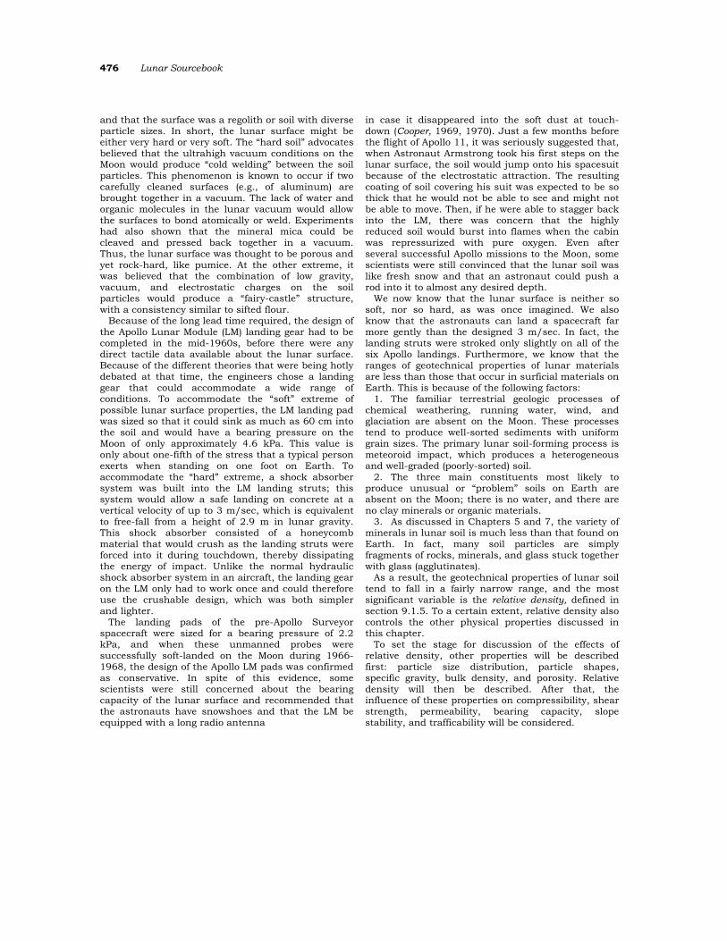
The principal method of determining the particle size distribution of an unconsolidated material is sieving, which is generally effective for particle sizes greater than about 10 µm. Scanning electron micro-scope (SEM) image analysis or Coulter counter methods are usually applied for measuring particle sizes that are smaller than 10 µm (Butler and King, 1974; McKay et al., 1974; Heiken, 1975). The particle size distribution can be presented graphically as histograms (as shown in Fig. 7.18b) or as cumulative curves, usually on log-probability plots (Fig. 9.1). Alternatively, the distribution may be characterized by parameters such as mean particle size, median particle size, sorting, skewness, and kurtosis, which are standard statistical measures for any grouped population (Folk, 1968; Koch and Link, 1970).
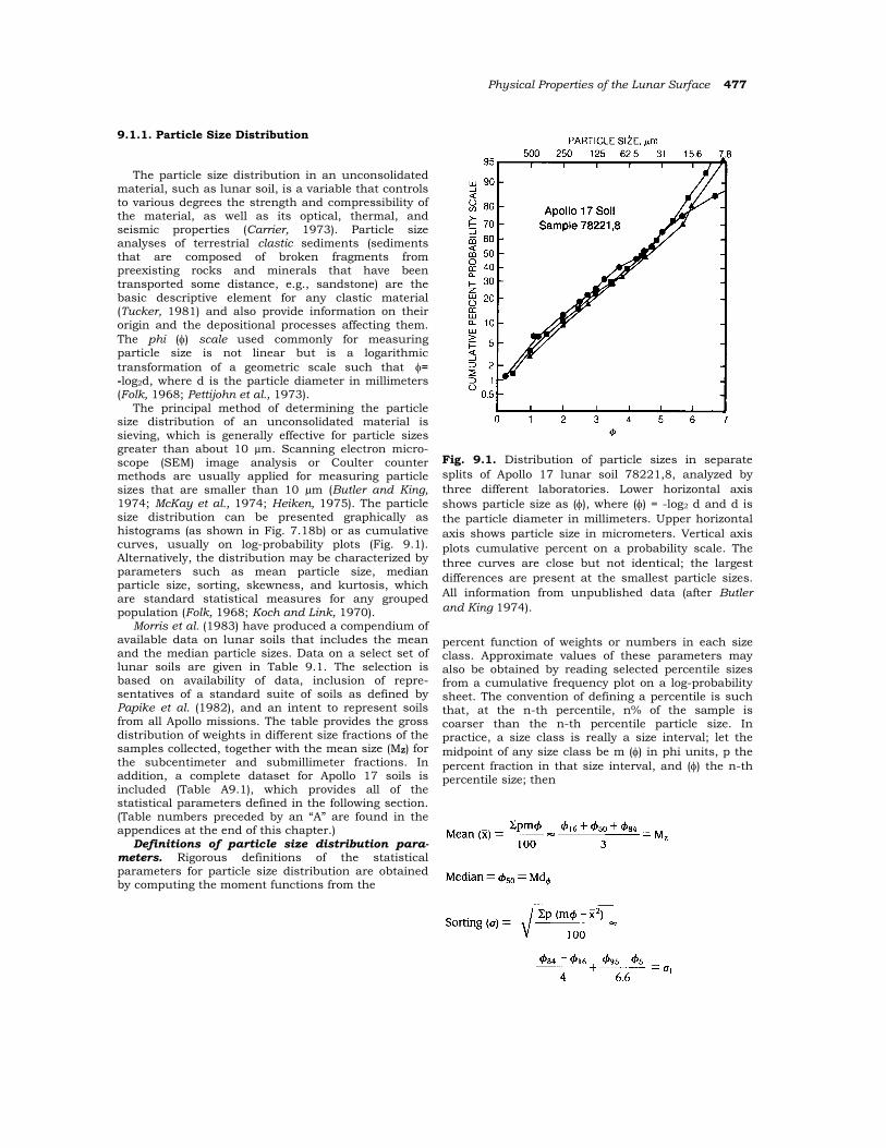
Morris et al. (1983) have produced a compendium of available data on lunar soils that includes the mean and the median particle sizes. Data on a select set of lunar soils are given in Table 9.1. The selection is based on availability of data, inclusion of repre-sentatives of a standard suite of soils as defined by Papike et al. (1982), and an intent to represent soils from all Apollo missions. The table provides the gross distribution of weights in different size fractions of the samples collected, together with the mean size (MZ) for the subcentimeter and submillimeter fractions. In addition, a complete dataset for Apollo 17 soils is included (Table A9.1), which provides all of the statistical parameters defined in the following section. (Table numbers preceded by an “A” are found in the appendices at the end of this chapter.)
Definitions of particle size distribution para-meters. Rigorous definitions of the statistical parameters for particle size distribution are obtained by computing the moment functions from the
Fig. 9.1. Distribution of particle sizes in separate splits of Apollo 17 lunar soil 78221,8, analyzed by three different laboratories. Lower horizontal axis shows particle size as (φ), where (φ) = -log2 d and d is the particle diameter in millimeters. Upper horizontal axis shows particle size in micrometers. Vertical axis plots cumulative percent on a probability scale. The three curves are close but not identical; the largest differences are present at the smallest particle sizes. All information from unpublished data (after Butler and King 1974).
percent function of weights or numbers in each size class. Approximate values of these parameters may also be obtained by reading selected percentile sizes from a cumulative frequency plot on a log-probability sheet. The convention of defining a percentile is such that, at the n-th percentile, n% of the sample is coarser than the n-th percentile particle size. In practice, a size class is really a size interval; let the midpoint of any size class be m (φ) in phi units, p the percent fraction in that size interval, and (φ) the n-th percentile size; then
478 Lunar Sourcebook
TABLE 9.1. Weight distribution in size fractions of representative scooped surface soils (from Morris et al., 1983; data emphasize coarser fractions).
Typical particle size distribution. The majority of
lunar soil samples fall in a fairly narrow range of particle-size distributions (Carrier, 1973). In general, the soil is a well-graded (or poorly sorted), silty sand to sandy silt: SW-SM to ML in the Unified Soil Classification System (ASTM D 2487, 1987; Lambe and Whitman, 1969). The median particle size is 40 to 130 µm, with an average of 70 µm; i.e., approximately half of the soil by weight is finer than the human eye can resolve. Roughly 10% to 20% of the soil is finer than 20 µm, and a thin layer of dust
adheres electrostatically to everything that comes in contact with the soil: spacesuits, tools, equipment, and lenses. Housekeeping is a major challenge for operations on the lunar surface. 9.1.2. Particle Shapes
The shapes of individual lunar soil particles are highly variable, ranging from spherical to extremely angular (Tables A9.2, A9.3, and A9.4; Fig. 7.2). In general, the particles are somewhat elongated and are subangular to angular. Because of the elongation, the particles tend to pack together with a preferred orientation of the long axes. This effect has been observed in lunar core tube samples and laboratory simulations, and the orientation has been found to be dependent on the mode of deposition (Mahmood et al., 1974a). Because of this preferred particle orientation, the physical properties of the lunar soil in situ are expected to be anisotropic. For example, the thermal conductivity in the horizontal direction should be different from that in the vertical direction. Furthermore, many of the particles are not compact, but have irregular, often reentrant surfaces. These particle surface irregularities especially affect the compressibility and shear strength of the soil, as discussed in more detail in sections 9.1.6 and 9.1.7.
Physical Properties of the Lunar Surface 479
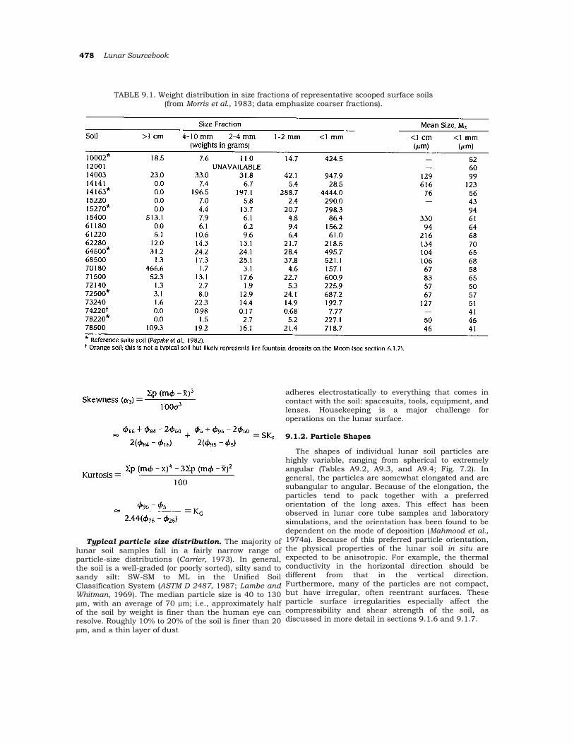
TABLE 9.2. Average particle shapes of lunar soil.
Thus, particle shape has a significant influence on bulk physical properties. Although shape is difficult to quantify, a number of measurements have been made, and the results are summarized in Table 9.2. The various shape parameters are discussed in the following sections.
Elongation. Elongation is defined as the ratio of the major to intermediate axes of the particle, or length to width. Particles with values of the ratio <1.3 are considered equant, and particles whose ratio is >1.3 are elongate.
Mahmood et al. (1974b) measured elongations of 1136 particles from three lunar soil samples (14163,148, 14259,3, and 15601,82). Individual particle sizes ranged from 2300 to <44 µm. The weighted average elongation ranged from 1.31 to 1.39. More details are given in Table A9.2.
Heywood (1971) measured elongation on 30 particles with a nominal size of 700 µm, all taken from one soil sample (12057,72). His values ranged from 1.32 to 1.38. Heywood also measured six other shape coefficients for these same particles: flatness, area ratio, volume coefficient, rugosity coefficient, specific circularity of profile, and specific circularity including the effect of rugosity. More details are given in Table A9.2.
Aspect ratio. In geotechnical studies, aspect ratio is inversely related to elongation; it is defined as the ratio of the minor axis to the major axis of an ellipse fitted to the particle by a least-squares approximation. Görz et al. (1971, 1972) measured aspect ratios on 2066 particles from seven lunar samples; particle sizes ranged from 1.25 to 30 µm. Values of the aspect ratios varied from 1.0 (equant) to <0.1 (very elongate), with most values falling in the range 0.4 to 0.7 (slightly-to-moderately elongated). Görz et al. (1972) also measured the shape complexity factor for most of these same particles. More details are given in Table A9.3.
Roundness. Roundness is defined as the ratio of the average of the radii of the corners of the particle image to the radius of the maximum inscribed circle. Mahmood et al. (1974b) measured roundness on silhouettes of the same 1136 particles for which they had measured elongation. The weighted average roundness values varied from 0.19 to 0.26, corres-ponding to subangular particle shapes. They also measured roundness in direct light on 641 particles from the same three lunar samples and found that the weighted average value varied from 0.20 to 0.25, corresponding to angular particles. More details are given in Table A9.4.
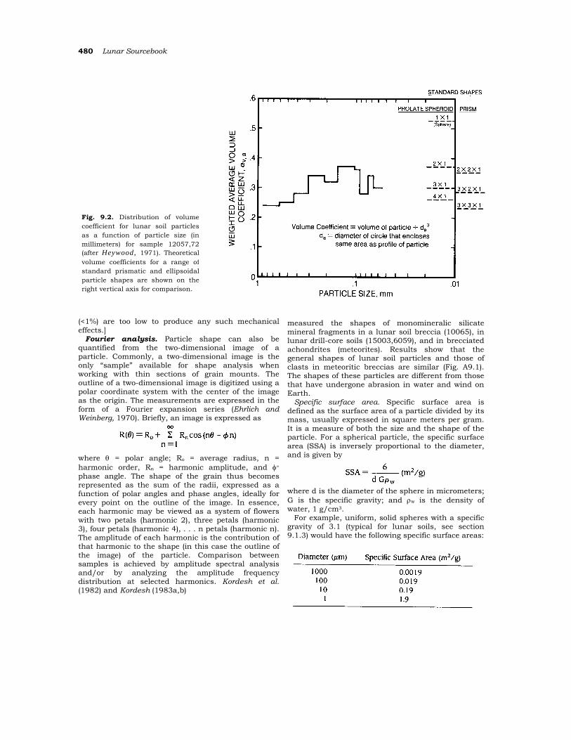
Volume coefficient. Volume coefficient is defined as the volume of a particle divided by the cube of the diameter of the circle that encloses the same area as the particle profile. Heywood (1971) determined the volume coefficient of 6755 particles taken from one Apollo 12 sample (12057,72); particle sizes ranged from 733 to 60 µm, which represents roughly the coarser half of a typical lunar soil sample. The results are plotted in Fig. 9.2, where it can be seen that the volume coefficient varies from 0.24 to 0.37, with an average value of about 0.3; this value corresponds approximately to a prolate spheroid with a major-to-minor axis ratio of 3 to 1.
The volume coefficient for a sphere is greater than 0.52, well above the measured values shown in Fig. 9.2. Heywood found that the glass spherules represent only about 1 in 500 particles in the coarse fraction of this Apollo 12 sample, and hence their effect on geotechnical properties is negligible. [Immediately after the Apollo 11 mission, some scientists had speculated that the “slipperiness” of the lunar soil reported by the astronauts was caused by the presence of a large proportion of such glass beads. This was even commented upon in the September 1969 issue of Scientific American. The observed amounts of such beads in most lunar soils
480 Lunar Sourcebook
(<1%) are too low to produce any such mechanical effects.]
Fourier analysis. Particle shape can also be quantified from the two-dimensional image of a particle. Commonly, a two-dimensional image is the only “sample” available for shape analysis when working with thin sections of grain mounts. The outline of a two-dimensional image is digitized using a polar coordinate system with the center of the image as the origin. The measurements are expressed in the form of a Fourier expansion series (Ehrlich and Weinberg, 1970). Briefly, an image is expressed as
where θ = polar angle; Ro = average radius, n = harmonic order, Rn = harmonic amplitude, and φ= phase angle. The shape of the grain thus becomes represented as the sum of the radii, expressed as a function of polar angles and phase angles, ideally for every point on the outline of the image. In essence, each harmonic may be viewed as a system of flowers with two petals (harmonic 2), three petals (harmonic 3), four petals (harmonic 4), . . . n petals (harmonic n). The amplitude of each harmonic is the contribution of that harmonic to the shape (in this case the outline of the image) of the particle. Comparison between samples is achieved by amplitude spectral analysis and/or by analyzing the amplitude frequency distribution at selected harmonics. Kordesh et al. (1982) and Kordesh (1983a,b)
measured the shapes of monomineralic silicate mineral fragments in a lunar soil breccia (10065), in lunar drill-core soils (15003,6059), and in brecciated achondrites (meteorites). Results show that the general shapes of lunar soil particles and those of clasts in meteoritic breccias are similar (Fig. A9.1). The shapes of these particles are different from those that have undergone abrasion in water and wind on Earth.
Specific surface area. Specific surface area is defined as the surface area of a particle divided by its mass, usually expressed in square meters per gram. It is a measure of both the size and the shape of the particle. For a spherical particle, the specific surface area (SSA) is inversely proportional to the diameter, and is given by
where d is the diameter of the sphere in micrometers; G is the specific gravity; and ρw is the density of water, 1 g/cm3.
For example, uniform, solid spheres with a specific gravity of 3.1 (typical for lunar soils, see section 9.1.3) would have the following specific surface areas:
Fig. 9.2. Distribution of volumecoefficient for lunar soil particlesas a function of particle size (inmillimeters) for sample 12057,72(after Heywood, 1971). Theoreticalvolume coefficients for a range ofstandard prismatic and ellipsoidalparticle shapes are shown on theright vertical axis for comparison.
Physical Properties of the Lunar Surface 481
A “soil” consisting of spheres with the same submillimeter particle size distribution as lunar soil would have a SSA of about 0.065 m2/g. This SSA value corresponds to an equivalent diameter of approximately 30 µm, which is less than the average particle size by weight of lunar soils (~65 µm). Because of the reciprocal relationship shown above, the smaller particles in a soil tend to contribute most to the bulk SSA value.
By comparison, terrestrial clay minerals have much higher SSA values, owing to their very small size and platy shape:
The results of 17 measurements of the SSA of lunar
soils are tabulated in Table A9.5 (Cadenhead et al., 1977). All these measurements were performed on the submillimeter soil fraction by means of nitrogen gas adsorption. The SSA values range from 0.02 to 0.78 m2/g, with a typical value of 0.5 m2/g, which corresponds to an equivalent spherical diameter of 3.9 µm. Hence, the SSA of lunar soil is much less than that of terrestrial clay minerals, and yet it is significantly greater than can be accounted for by small particle sizes alone. Rather, the relatively large SSA of lunar soils is indicative of the extremely irregular, reentrant particle shapes.
These considerations suggest in turn the definition for a new shape parameter that is independent of the particle size, which is called the equivalent surface area ratio (ESAR)
where ds = equivalent diameter of spheres with the same particle size distribution as the soil being tested and de = equivalent spherical diameter of the soil, as calculated from the specific surface area.
For a typical lunar soil, the equivalent surface area ratio would be nearly 8; that is, the soil would have eight times as much surface area as would an assemblage of spheres with the equivalent particle size distribution. 9.1.3. Specific Gravity
The specific gravity, G, of a soil particle is defined as the ratio of its mass to the mass of an equal volume of water at 4°C. Many terrestrial soils have a specific gravity of 2.7; that is, the density of the individual particles is 2.7 g/cm3, or 2.7 times that of water (1 g/cm3).
In order to determine the specific gravity of a soil, a portion of the material is first weighed, and then immersed in a fluid to measure the volume that it displaces. Various fluids can be used, including water, air, or helium. The specific gravity of lunar soils, breccias, and individual rock fragments has been measured by various investigators, and the results are summarized in Table 9.3. Values for lunar soils range from 2.3 to >3.2; we recommend a value of 3.1 for general scientific and engineering analyses of lunar soils.
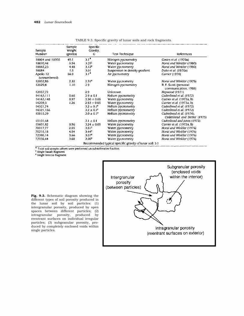
The average specific gravity of a given lunar soil is related to the relative proportions of different particle types; i.e., basalts, mineral fragments, breccias, agglutinates, and glasses (Fig. 7.1). However, the interpretation of the specific gravity is complicated by the porosity of the particles. As illustrated in Fig. 9.3, the porosity may be divided into three categories: (1) intergranular porosity, or the volume of space between individual particles; (2) intragranular porosity, or the volume of reentrant surfaces on the exterior of the particles; and (3) subgranular porosity, or the volume of enclosed voids within the interior of particles.
When the soil particles are immersed in a fluid, the intergranular and intragranular space is filled, but not the subgranular space. Thus, the measured specific gravity is not solely an index of particle mineralogy, but also includes the effect of enclosed voids. By suspending the soil particles in a density gradient, produced by varying the proportions of a mixture of methylene iodine and dimethyl formamide, Duke et al. (1970b) found the following values of specific gravity:
Agglutinate and glass particles 1.0 to >3.32 Basalt particles >3.32 Breccia particles 2.9 to 3.10
The enclosed voids in a lunar soil particle with a
specific gravity of 1.0 occupy two-thirds of the total volume of the particle. Thus, the average specific gravity of the particles would be even greater if there were no enclosed voids. For example, if the lunar soil were ground into a fine powder (in which the resulting particles were smaller than the enclosed voids), these voids would be destroyed, and the specific gravity would be increased. The actual subgranular porosity of individual lunar soil particles is only poorly known, and additional measurements of subgranular porosity are needed.
The intragranular porosity has a strong effect on the bulk density of the lunar soil, whereas the intergranular porosity affects both the bulk density and the relative density. These relations will be discussed in more detail in the following sections.
482 Lunar Sourcebook
TABLE 9.3. Specific gravity of lunar soils and rock fragments.
Fig. 9.3. Schematic diagram showing the different types of soil porosity produced in the lunar soil by soil particles: (1) intergranular porosity, produced by open spaces between different particles; (2) intragranular porosity, produced by reentrant surfaces on individual irregular particles; (3) subgranular porosity, pro-duced by completely enclosed voids within single particles.
Physical Properties of the Lunar Surface 483
9.1.4. Bulk Density and Porosity
The bulk density, ρ, of soil is defined as the mass of the material contained within a given volume, usually expressed in grams per cubic centimer. The porosity, n, is defined as the volume of void space between the particles divided by the total volume. Bulk density, porosity, and specific gravity are interrelated as
where G = specific gravity (including subgranular porosity; section 9.1.3); ρw = density of water = 1 g/cm3; and n = porosity, expressed as a decimal (combining both inter- and intragranular porosity).
It is convenient in geotechnical engineering to also define another parameter, the void ratio, which is equal to the volume of void space between the particles divided by the volume of the “solid” particles (again, including the subgranular porosity). Void ratio, e, and porosity are interrelated as
The in situ bulk density of lunar soil is a funda-mental property. It influences bearing capacity, slope stability, seismic velocity, thermal conductivity, electrical resistivity, and the depth of penetration of ionizing radiation. Consequently, considerable effort has been expended over the years in obtaining estimates of this important parameter.
Prior to the soft landings on the Moon, remote-sensing techniques were used to infer the bulk density of the lunar soil. These techniques included passive measurements of optical, infrared, and microwave emissivity and active measurements of radar reflectivity. With the Surveyor and Luna unmanned landings, direct measurements were possible at discrete points. In addition, correlations with laboratory tests on simulated lunar soil permitted extrapolation over wider areas. Finally, beginning with Apollo, core tube samples of lunar soil were returned that permitted unambiguous measurements of the in situ bulk density. At present, the best estimate for the average bulk density of the top 15 cm of lunar soil is 1.50 ± 0.05 g/cm3, and of the top 60 cm, 1.66 ± 0.05 g/cm3 (Mitchell et al., 1974).
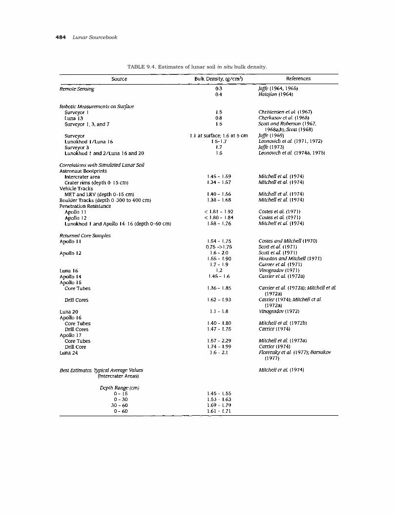
A summary of estimated lunar bulk densities is presented in Table 9.4, together with recommended typical values. The various estimating and measuring techniques are described in the following sections.
Early inferred values of bulk density based on remote sensing. As shown in Table 9.4, a very low density of 0.3 g/cm3 was assumed by Jaffe (1964,
1965) in an effort to estimate lower-bound bearing capacities. Halajian (1964) also assumed a very low density of 0.4 g/cm3, but believed that the strength of the lunar surface was similar to that of pumice.
Robotic measurements of bulk density on the lunar surface. When Surveyor 1 landed on the Moon in June 1966, a much higher density of 1.5 g/ cm3 was deduced by Christensen et al. (1967), using records of the interaction between the lunar soil and the spacecraft footpads, combined with analysis of the television images, to determine the particle size distribution. Shortly thereafter, the first in situ measurement of lunar soil density was made by the U.S.S.R. probe, Luna 13, using a gamma-ray device. The calibration curve for this device was double-valued, and the data obtained were consistent with two density values: 0.8 and 2.1 g/cm3; Cherkasov et al. (1968) chose the lesser value. Based on the results from the soil mechanics surface sampler experiments on Surveyor 3 and 7, Scott and Roberson (1967, 1968a,b) confirmed the Surveyor 1 value of 1.5 g/cm3, and Scott (1968) suggested that the Soviet investigators had chosen the wrong portion of their calibration curve. Just before the Apollo 11 landing, Jaffe (1969) reevaluated the Surveyor data and proposed that the bulk density was 1.1 g/cm3 at the surface and increased linearly to 1.6 g/cm3 at a depth of 5 cm.
Later, during the early 1970s, the U.S.S.R. unmanned roving vehicles Lunokhod 1 and Lunokhod 2 traversed a total of 47 km on the lunar surface. These vehicles performed approximately 1000 cone-vane penetrometer tests to depths of 10 cm (see section 9.1.7). Leonovich et al. (1974a, 1975) correlated the lunar surface penetration resistance with measurements on returned lunar samples from Luna 16 and Luna 20, and they deduced an average surficial bulk density of about 1.5 g/cm3.
Inferred values of bulk density based on correlations with simulated lunar soil. The in situ bulk density of lunar soil has also been estimated from analyses of astronaut bootprints, vehicle tracks, boulder tracks, and penetration resistance. The results are summarized in Table 9.4. Mitchell et al. (1974) found that the astronaut bootprints indicated a density of approximately 1.45 to 1.59 g/cm3, representative of the top 15 cm of the lunar surface in the intercrater areas. The soils on crater rims were found to be slightly less dense: 1.34 to 1.57 g/cm3. Analysis of vehicle tracks made by the Modular Equipment Transporter (Apollo 14) and the Lunar Roving Vehicle (Apollo 15, 16, and 17) indicated values of 1.40 to 1.56 g/cm3, also representative of the top 15 cm. The tracks left by boulders that had rolled downslope at the Apollo 17 site indicated a density of 1.38 to 1.68 g/cm3,
484 Lunar Sourcebook
TABLE 9.4. Estimates of lunar soil in situ bulk density.
Physical Properties of the Lunar Surface 485
representative of the top 300 to 400 cm of the regolith (Mitchell et al., 1974). Costes et al. (1971) analyzed the resistance of the soil to penetration by the flagpole, the Solar Wind Composition Experiment staff, and other tools at the Apollo 11 and 12 sites; they deduced upper limits for the densities of 1.81 to 1.92 g/cm3 and 1.80 to 1.84 g/cm3, respectively. Finally, Mitchell et al. (1974) found that penetrometer measurements made by Lunokhod 1 and on the Apollo 14, 15, and 16 missions indicated densities of 1.58 to 1.76 g/cm3, representative of the top 60 cm.
In each of the above analyses, it was necessary to assume that the lunar soil behaves approximately the same as a simulant of crushed basaltic lava with a similar particle size distribution, after correction for the effect of gravity. These correlations were developed by normalizing with respect to relative density (see section 9.1.5). During the early Apollo. missions, when very little data were available, it was necessary to assume that both the specific gravity and maximum and minimum porosity values for lunar soil were the same as for the simulant. Later, it became clear that this was not the case. Hence, these interpretive methods are better estimators of relative density than of bulk density, and will be discussed in more detail in section 9.1.5.
Measurements of bulk density on returned core samples. Beginning with the Apollo 11 mission, core tube samples of lunar soil were collected and returned from all of the Apollo sites and three of the Luna sites. Such cores are important because they provide a more or less continuous section into the uppermost lunar regolith, to depths up to 3 m.
Two different types of coring tools were used to sample the regolith: Drive core tubes were hollow tubes hammered vertically into the regolith by an astronaut to depths of less than a meter. Rotary drill core tubes were drilled into the surface to depths of several meters.
Altogether, nearly 16 kg of drive core tube materials have been recovered, using core tubes driven to depths of approximately 70 cm into the lunar surface. In addition, more than 4 kg of rotary drill
core tube samples have been recovered, from depths of up to 3 m. Density data for these samples are summarized in Tables A9.6 and A9.7, respectively.
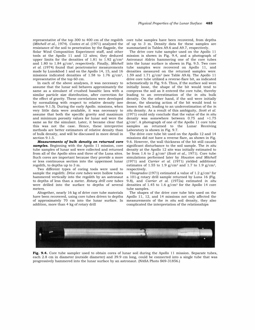
The drive core tube sampler used on the Apollo 11 mission is shown in Fig. 9.4, and a photograph of Astronaut Aldrin hammering one of the core tubes into the lunar surface is shown in Fig. 9.5. Two core tube samples were recovered on Apollo 11, and densities measured on the returned samples were. 1.59 and 1.71 g/cm3 (see Table A9.6). The Apollo 11 drive core tube utilized a reverse-flare bit, as indicated schematically in Fig. 9.6. Thus, if the surface soil were initially loose, the shape of the bit would tend to compress the soil as it entered the core tube, thereby leading to an overestimation of the in situ bulk density. On the other hand, if the soil were initially dense, the shearing action of the bit would tend to loosen the soil, leading to an underestimation of the in situ density. As a result of this ambiguity, Scott et al. (1971) could only conclude that the value of the in situ density was somewhere between 0.75 and >1.75 g/cm3. A photograph of one of the Apollo 11 core tube samples as returned to the Lunar Receiving Laboratory is shown in Fig. 9.7.
The drive core tube bit used on the Apollo 12 and 14 missions did not have a reverse flare, as shown in Fig. 9.6. However, the wall thickness of the bit still caused significant disturbance to the soil sample. The in situ density at the Apollo 12 site was initially estimated to be from 1.6 to 2 g/cm3 (Scott et al., 1971). Core tube simulations performed later by Houston and Mitchell (1971) and Carrier et al. (1971) yielded additional estimates of 1.55 to 1.9 g/cm3 and 1.7 to 1.9 g/cm3, respectively.
Vinogradov (1971) estimated a value of 1.2 g/cm3 for a 101-g rotary drill sample returned by Luna 16 (Fig. 9.8), and Carrier et al. (1972a) estimated in situ densities of 1.45 to 1.6 g/cm3 for the Apollo 14 core tube samples.
The shapes of the drive core tube bits used on the Apollo 11, 12, and 14 missions not only affected the measurements of the in situ soil density, they also complicated the interpretation of the relationships
Fig. 9.4. Core tube sampler used to obtain cores of lunar soil during the Apollo 11 mission. Separate tubes, each 2.8 cm in diameter (outside diameter) and 39.9 cm long, could be connected into a single tube that was progressively hammered into the lunar surface by an astronaut. (NASA Photo S69-31856.)
486 Lunar Sourcebook
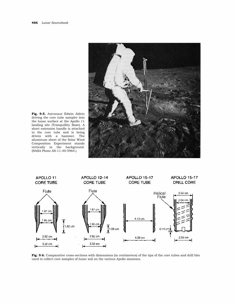
Fig. 9.5. Astronaut Edwin Aldrin driving the core tube sampler into the lunar surface at the Apollo 11 landing site (Tranquillity Base). A short extension handle is attached to the core tube and is being driven with a hammer. The aluminum sheet of the Solar Wind Composition Experiment stands vertically in the background. (NASA Photo AS-11-40-5964.)
Fig. 9.6. Comparative cross-sections with dimensions (in centimeters) of the tips of the core tubes and drill bits used to collect core samples of lunar soil on the various Apollo missions.
Physical Properties of the Lunar Surface 487
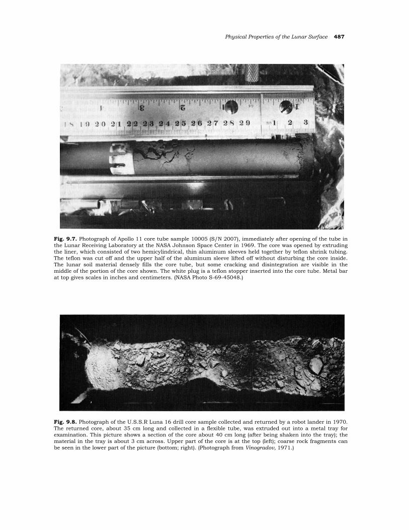
Fig. 9.7. Photograph of Apollo 11 core tube sample 10005 (S/N 2007), immediately after opening of the tube in the Lunar Receiving Laboratory at the NASA Johnson Space Center in 1969. The core was opened by extruding the liner, which consisted of two hemicylindrical, thin aluminum sleeves held together by teflon shrink tubing. The teflon was cut off and the upper half of the aluminum sleeve lifted off without disturbing the core inside. The lunar soil material densely fills the core tube, but some cracking and disintegration are visible in the middle of the portion of the core shown. The white plug is a teflon stopper inserted into the core tube. Metal bar at top gives scales in inches and centimeters. (NASA Photo S-69-45048.)
Fig. 9.8. Photograph of the U.S.S.R Luna 16 drill core sample collected and returned by a robot lander in 1970. The returned core, about 35 cm long and collected in a flexible tube, was extruded out into a metal tray for examination. This picture shows a section of the core about 40 cm long (after being shaken into the tray); the material in the tray is about 3 cm across. Upper part of the core is at the top (left); coarse rock fragments can be seen in the lower part of the picture (bottom; right). (Photograph from Vinogradov, 1971.)
488 Lunar Sourcebook
between density and depth. The problem arises from the fact that a depth of, e.g., 50 cm in an early Apollo core tube sample does not correspond to the same depth below the lunar surface. In general, the sample lengths in the core tube are less than the depths to which the cores were driven. These discrepancies arise from the process by which the core tubes penetrated the soil as they were hammered in. As the core tube penetrates the surface, a portion of the soil enters the tube and a portion is pushed outward; the portion that enters the tube may be either compressed or loosened. As the depth increases, the portion entering the tube progressively decreases until no more sample is recovered; the tube is now plugged, and the deeper soil is simply pushed aside. Detailed laboratory simulations were performed with the Apollo 11, 12, and 14 core tubes, and approximate depth calibrations were developed by Carrier et al. (1971, 1972a). The results are summarized in Fig. A9.2.
The same types of laboratory simulations were used to evaluate the depth relationships for the rotary drill cores used on the Apollo 15, 16, and 17 missions. In some of these returned core samples, the interpretation was complicated by obvious
sample disturbance in some of the drill stems (tubes). Depth estimates were developed by Carrier (1974) and are summarized in Fig. A9.3.
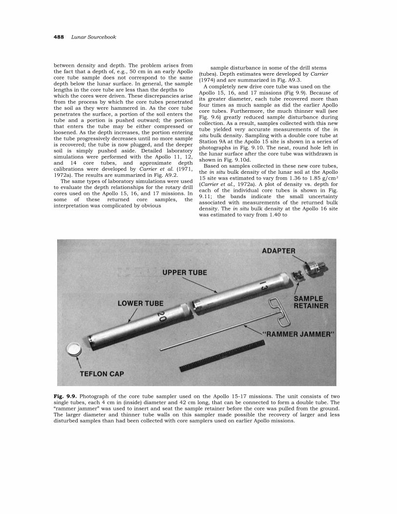
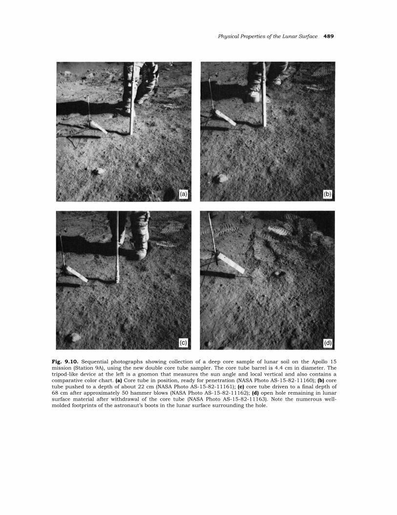
A completely new drive core tube was used on the Apollo 15, 16, and 17 missions (Fig 9.9). Because of its greater diameter, each tube recovered more than four times as much sample as did the earlier Apollo core tubes. Furthermore, the much thinner wall (see Fig. 9.6) greatly reduced sample disturbance during collection. As a result, samples collected with this new tube yielded very accurate measurements of the in situ bulk density. Sampling with a double core tube at Station 9A at the Apollo 15 site is shown in a series of photographs in Fig. 9.10. The neat, round hole left in the lunar surface after the core tube was withdrawn is shown in Fig. 9.10d.
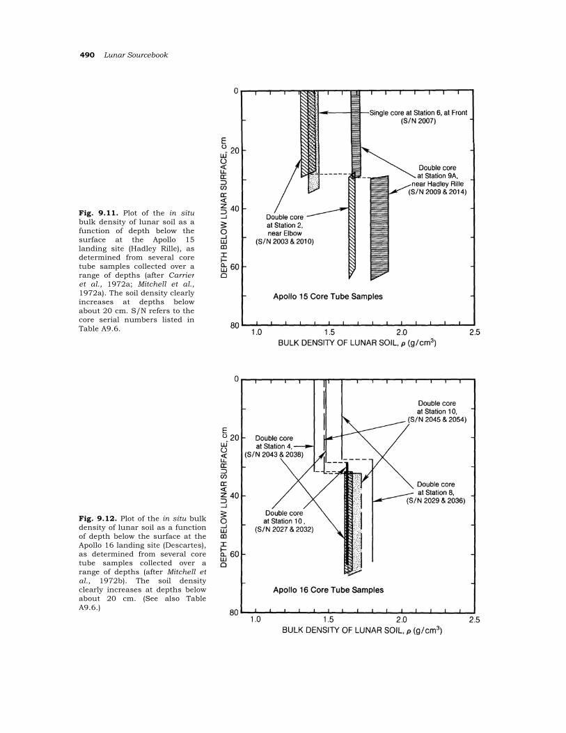
Based on samples collected in these new core tubes, the in situ bulk density of the lunar soil at the Apollo 15 site was estimated to vary from 1.36 to 1.85 g/cm3 (Carrier et al., 1972a). A plot of density vs. depth for each of the individual core tubes is shown in Fig. 9.11; the bands indicate the small uncertainty associated with measurements of the returned bulk density. The in situ bulk density at the Apollo 16 site was estimated to vary from 1.40 to
Fig. 9.9. Photograph of the core tube sampler used on the Apollo 15-17 missions. The unit consists of two single tubes, each 4 cm in (inside) diameter and 42 cm long, that can be connected to form a double tube. The “rammer jammer” was used to insert and seat the sample retainer before the core was pulled from the ground. The larger diameter and thinner tube walls on this sampler made possible the recovery of larger and less disturbed samples than had been collected with core samplers used on earlier Apollo missions.
Physical Properties of the Lunar Surface 489
Fig. 9.10. Sequential photographs showing collection of a deep core sample of lunar soil on the Apollo 15 mission (Station 9A), using the new double core tube sampler. The core tube barrel is 4.4 cm in diameter. The tripod-like device at the left is a gnomon that measures the sun angle and local vertical and also contains a comparative color chart. (a) Core tube in position, ready for penetration (NASA Photo AS-15-82-11160); (b) core tube pushed to a depth of about 22 cm (NASA Photo AS-15-82-11161); (c) core tube driven to a final depth of 68 cm after approximately 50 hammer blows (NASA Photo AS-15-82-11162); (d) open hole remaining in lunar surface material after withdrawal of the core tube (NASA Photo AS-15-82-11163). Note the numerous well-molded footprints of the astronaut’s boots in the lunar surface surrounding the hole.
490 Lunar Sourcebook
Fig. 9.11. Plot of the in situbulk density of lunar soil as afunction of depth below thesurface at the Apollo 15landing site (Hadley Rille), asdetermined from several coretube samples collected over arange of depths (after Carrieret al., 1972a; Mitchell et al.,1972a). The soil density clearlyincreases at depths belowabout 20 cm. S/N refers to thecore serial numbers listed inTable A9.6.
Fig. 9.12. Plot of the in situ bulkdensity of lunar soil as a functionof depth below the surface at theApollo 16 landing site (Descartes),as determined from several coretube samples collected over arange of depths (after Mitchell etal., 1972b). The soil densityclearly increases at depths belowabout 20 cm. (See also TableA9.6.)
Physical Properties of the Lunar Surface 491
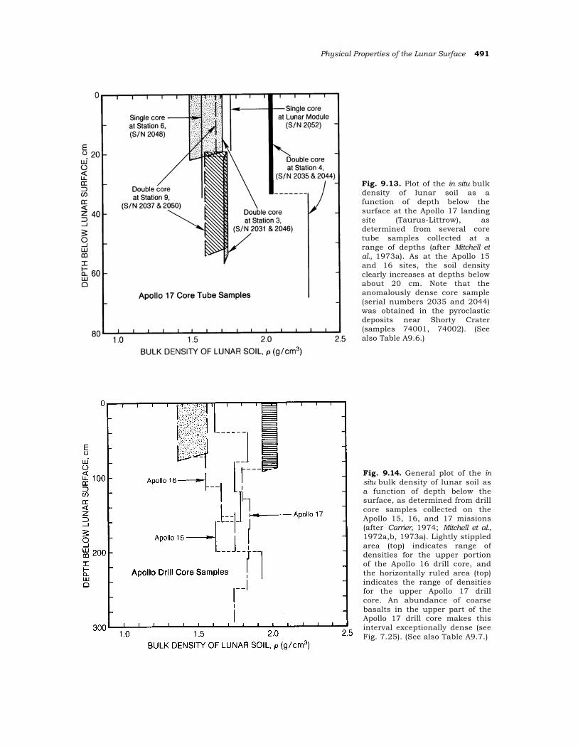
Fig. 9.13. Plot of the in situ bulkdensity of lunar soil as afunction of depth below thesurface at the Apollo 17 landingsite (Taurus-Littrow), asdetermined from several coretube samples collected at arange of depths (after Mitchell etal., 1973a). As at the Apollo 15and 16 sites, the soil densityclearly increases at depths belowabout 20 cm. Note that theanomalously dense core sample(serial numbers 2035 and 2044)was obtained in the pyroclasticdeposits near Shorty Crater(samples 74001, 74002). (Seealso Table A9.6.)
Fig. 9.14. General plot of the insitu bulk density of lunar soil asa function of depth below thesurface, as determined from drillcore samples collected on theApollo 15, 16, and 17 missions(after Carrier, 1974; Mitchell et al.,1972a,b, 1973a). Lightly stippledarea (top) indicates range ofdensities for the upper portionof the Apollo 16 drill core, andthe horizontally ruled area (top)indicates the range of densitiesfor the upper Apollo 17 drillcore. An abundance of coarsebasalts in the upper part of theApollo 17 drill core makes thisinterval exceptionally dense (seeFig. 7.25). (See also Table A9.7.)
492 Lunar Sourcebook
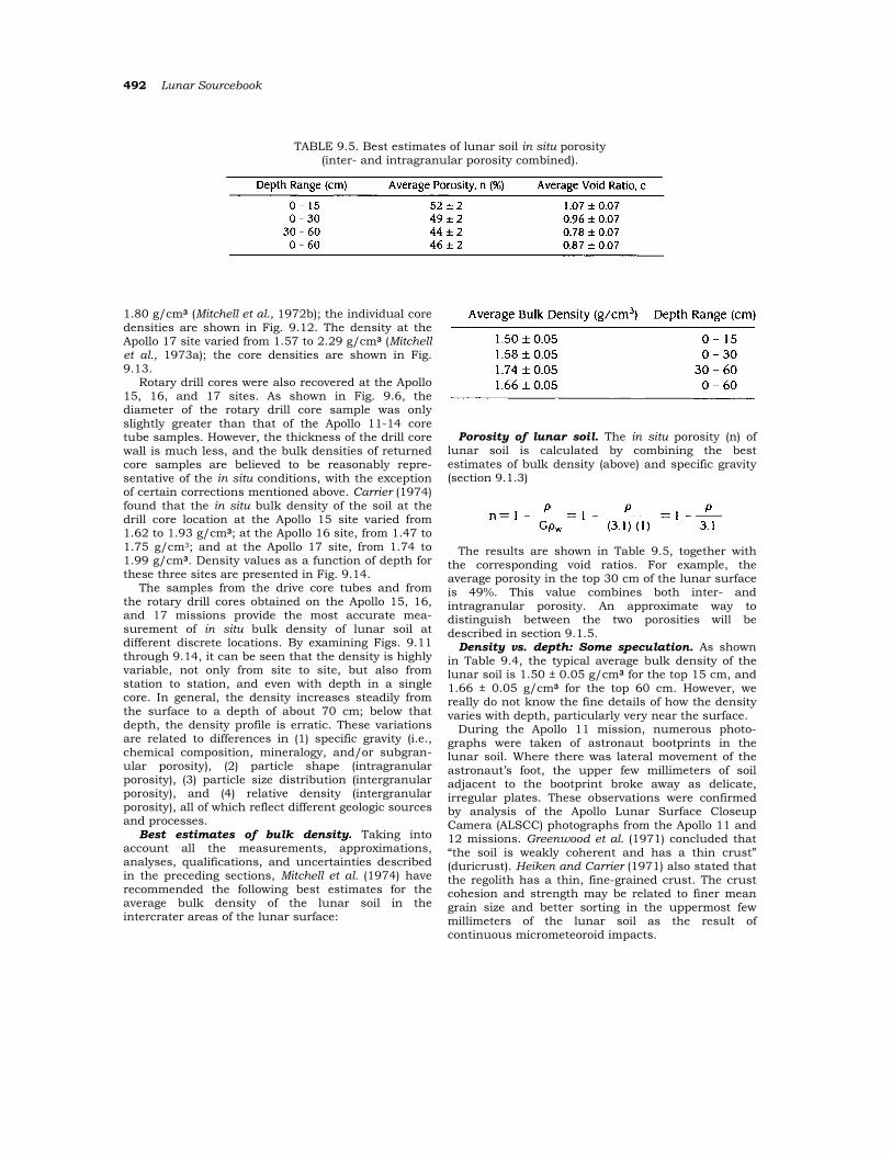
TABLE 9.5. Best estimates of lunar soil in situ porosity (inter- and intragranular porosity combined).
1.80 g/cm3 (Mitchell et al., 1972b); the individual core densities are shown in Fig. 9.12. The density at the Apollo 17 site varied from 1.57 to 2.29 g/cm3 (Mitchell et al., 1973a); the core densities are shown in Fig. 9.13.
Rotary drill cores were also recovered at the Apollo 15, 16, and 17 sites. As shown in Fig. 9.6, the diameter of the rotary drill core sample was only slightly greater than that of the Apollo 11-14 core tube samples. However, the thickness of the drill core wall is much less, and the bulk densities of returned core samples are believed to be reasonably repre-sentative of the in situ conditions, with the exception of certain corrections mentioned above. Carrier (1974) found that the in situ bulk density of the soil at the drill core location at the Apollo 15 site varied from 1.62 to 1.93 g/cm3; at the Apollo 16 site, from 1.47 to 1.75 g/cm3; and at the Apollo 17 site, from 1.74 to 1.99 g/cm3. Density values as a function of depth for these three sites are presented in Fig. 9.14.
The samples from the drive core tubes and from the rotary drill cores obtained on the Apollo 15, 16, and 17 missions provide the most accurate mea-surement of in situ bulk density of lunar soil at different discrete locations. By examining Figs. 9.11 through 9.14, it can be seen that the density is highly variable, not only from site to site, but also from station to station, and even with depth in a single core. In general, the density increases steadily from the surface to a depth of about 70 cm; below that depth, the density profile is erratic. These variations are related to differences in (1) specific gravity (i.e., chemical composition, mineralogy, and/or subgran-ular porosity), (2) particle shape (intragranular porosity), (3) particle size distribution (intergranular porosity), and (4) relative density (intergranular porosity), all of which reflect different geologic sources and processes.
Best estimates of bulk density. Taking into account all the measurements, approximations, analyses, qualifications, and uncertainties described in the preceding sections, Mitchell et al. (1974) have recommended the following best estimates for the average bulk density of the lunar soil in the intercrater areas of the lunar surface:
Porosity of lunar soil. The in situ porosity (n) of
lunar soil is calculated by combining the best estimates of bulk density (above) and specific gravity (section 9.1.3)
The results are shown in Table 9.5, together with
the corresponding void ratios. For example, the average porosity in the top 30 cm of the lunar surface is 49%. This value combines both inter- and intragranular porosity. An approximate way to distinguish between the two porosities will be described in section 9.1.5.
Density vs. depth: Some speculation. As shown in Table 9.4, the typical average bulk density of the lunar soil is 1.50 ± 0.05 g/cm3 for the top 15 cm, and 1.66 ± 0.05 g/cm3 for the top 60 cm. However, we really do not know the fine details of how the density varies with depth, particularly very near the surface.
During the Apollo 11 mission, numerous photo-graphs were taken of astronaut bootprints in the lunar soil. Where there was lateral movement of the astronaut’s foot, the upper few millimeters of soil adjacent to the bootprint broke away as delicate, irregular plates. These observations were confirmed by analysis of the Apollo Lunar Surface Closeup Camera (ALSCC) photographs from the Apollo 11 and 12 missions. Greenwood et al. (1971) concluded that “the soil is weakly coherent and has a thin crust” (duricrust). Heiken and Carrier (1971) also stated that the regolith has a thin, fine-grained crust. The crust cohesion and strength may be related to finer mean grain size and better sorting in the uppermost few millimeters of the lunar soil as the result of continuous micrometeoroid impacts.
Physical Properties of the Lunar Surface 493
Another hypothesis is that the uppermost soil layer is sorted during the process of thermal solifluction (Shoemaker et al., 1968).
The presence of a thin soil crust was questioned by Jaffe (1971b), who had observed similar features on the regolith surface around the Surveyor landers. He proposed that the thin plates were artifacts produced by the lighting angle at which the pictures were taken and that the “lunar duricrust” does not exist. However, the ALSCC photographs confirm the presence of such a crust at the Apollo 11 and 12 sites. Furthermore, during dissection of the Apollo core tubes, thin, blocky “clods” were observed, each being slightly more cohesive and finer-grained than the surrounding soil. It is possible that these clods are remnants of lunar duricrust, broken by microme-teoroid impacts and mixed into the underlying regolith.
Below the top few millimeters of lunar soil, the Apollo drive core tube and rotary drill core data presented in Figs. 9.11 through 9.14 can be used to establish certain constraints on the density profile:
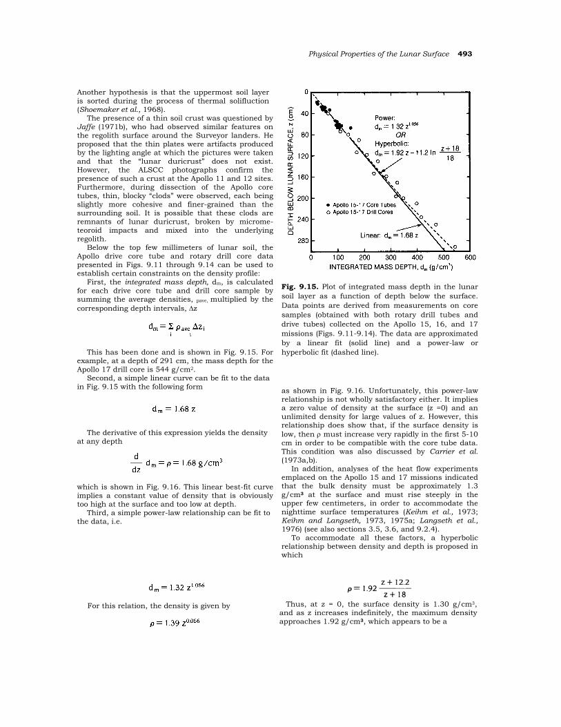
First, the integrated mass depth, dm, is calculated for each drive core tube and drill core sample by summing the average densities, pave, multiplied by the corresponding depth intervals, ∆z
This has been done and is shown in Fig. 9.15. For example, at a depth of 291 cm, the mass depth for the Apollo 17 drill core is 544 g/cm2.
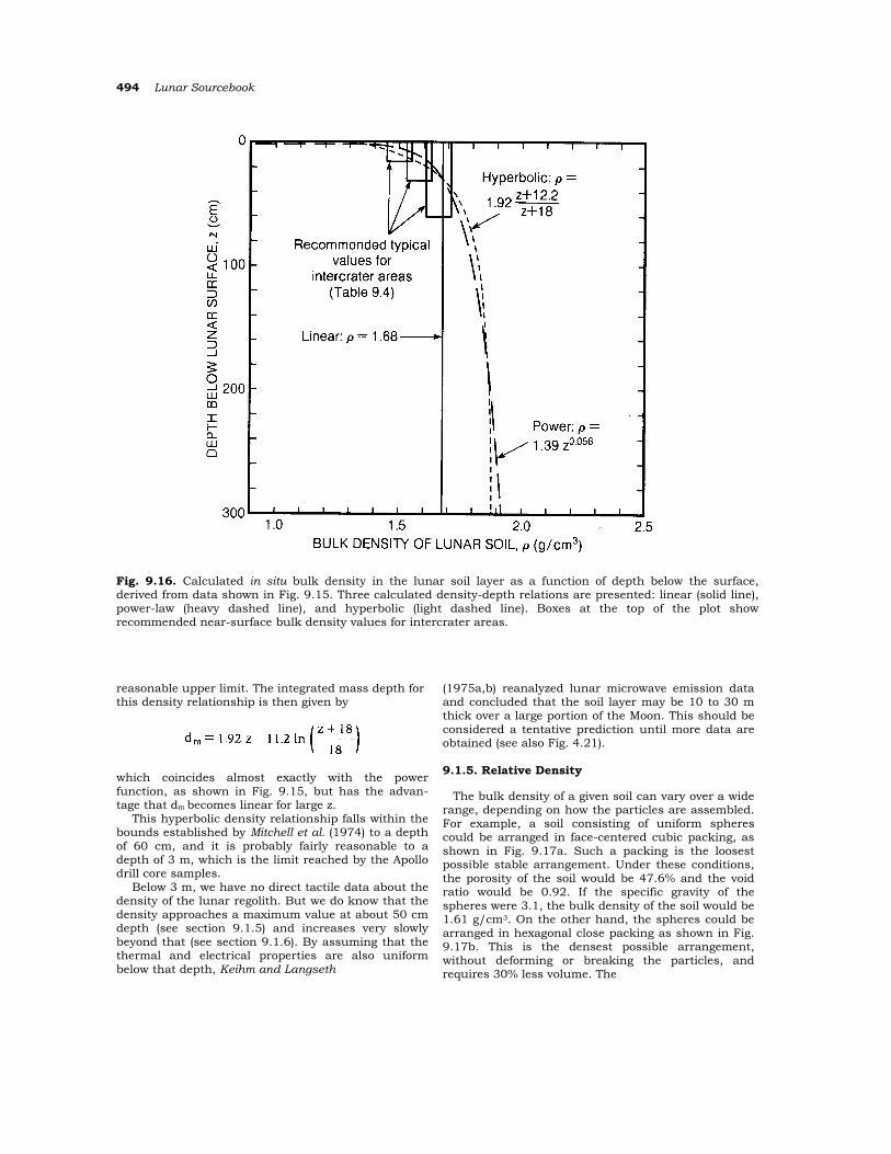
Second, a simple linear curve can be fit to the data in Fig. 9.15 with the following form
The derivative of this expression yields the density at any depth
which is shown in Fig. 9.16. This linear best-fit curve implies a constant value of density that is obviously too high at the surface and too low at depth.
Third, a simple power-law relationship can be fit to the data, i.e.
Fig. 9.15. Plot of integrated mass depth in the lunar soil layer as a function of depth below the surface. Data points are derived from measurements on core samples (obtained with both rotary drill tubes and drive tubes) collected on the Apollo 15, 16, and 17 missions (Figs. 9.11-9.14). The data are approximated by a linear fit (solid line) and a power-law or hyperbolic fit (dashed line).
as shown in Fig. 9.16. Unfortunately, this power-law relationship is not wholly satisfactory either. It implies a zero value of density at the surface (z =0) and an unlimited density for large values of z. However, this relationship does show that, if the surface density is low, then ρ must increase very rapidly in the first 5-10 cm in order to be compatible with the core tube data. This condition was also discussed by Carrier et al. (1973a,b).
In addition, analyses of the heat flow experiments emplaced on the Apollo 15 and 17 missions indicated that the bulk density must be approximately 1.3 g/cm3 at the surface and must rise steeply in the upper few centimeters, in order to accommodate the nighttime surface temperatures (Keihm et al., 1973; Keihm and Langseth, 1973, 1975a; Langseth et al., 1976) (see also sections 3.5, 3.6, and 9.2.4).
To accommodate all these factors, a hyperbolic relationship between density and depth is proposed in which
For this relation, the density is given by
Thus, at z = 0, the surface density is 1.30 g/cm3, and as z increases indefinitely, the maximum density approaches 1.92 g/cm3, which appears to be a
494 Lunar Sourcebook
Fig. 9.16. Calculated in situ bulk density in the lunar soil layer as a function of depth below the surface, derived from data shown in Fig. 9.15. Three calculated density-depth relations are presented: linear (solid line), power-law (heavy dashed line), and hyperbolic (light dashed line). Boxes at the top of the plot show recommended near-surface bulk density values for intercrater areas.
reasonable upper limit. The integrated mass depth for this density relationship is then given by
which coincides almost exactly with the power function, as shown in Fig. 9.15, but has the advan-tage that dm becomes linear for large z.
This hyperbolic density relationship falls within the bounds established by Mitchell et al. (1974) to a depth of 60 cm, and it is probably fairly reasonable to a depth of 3 m, which is the limit reached by the Apollo drill core samples.
Below 3 m, we have no direct tactile data about the density of the lunar regolith. But we do know that the density approaches a maximum value at about 50 cm depth (see section 9.1.5) and increases very slowly beyond that (see section 9.1.6). By assuming that the thermal and electrical properties are also uniform below that depth, Keihm and Langseth
(1975a,b) reanalyzed lunar microwave emission data and concluded that the soil layer may be 10 to 30 m thick over a large portion of the Moon. This should be considered a tentative prediction until more data are obtained (see also Fig. 4.21). 9.1.5. Relative Density
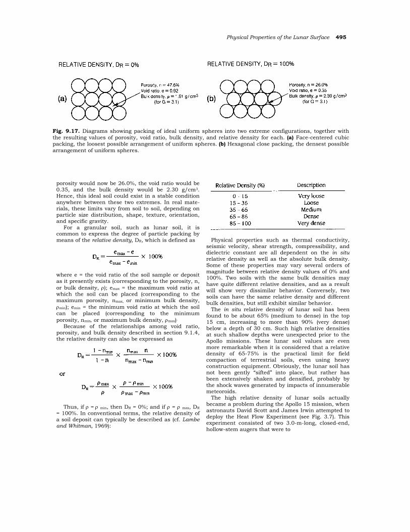
The bulk density of a given soil can vary over a wide range, depending on how the particles are assembled. For example, a soil consisting of uniform spheres could be arranged in face-centered cubic packing, as shown in Fig. 9.17a. Such a packing is the loosest possible stable arrangement. Under these conditions, the porosity of the soil would be 47.6% and the void ratio would be 0.92. If the specific gravity of the spheres were 3.1, the bulk density of the soil would be 1.61 g/cm3. On the other hand, the spheres could be arranged in hexagonal close packing as shown in Fig. 9.17b. This is the densest possible arrangement, without deforming or breaking the particles, and requires 30% less volume. The
Physical Properties of the Lunar Surface 495
Fig. 9.17. Diagrams showing packing of ideal uniform spheres into two extreme configurations, together with the resulting values of porosity, void ratio, bulk density, and relative density for each. (a) Face-centered cubic packing, the loosest possible arrangement of uniform spheres. (b) Hexagonal close packing, the densest possible arrangement of uniform spheres.
porosity would now be 26.0%, the void ratio would be 0.35, and the bulk density would be 2.30 g/cm3. Hence, this ideal soil could exist in a stable condition anywhere between these two extremes. In real mate-rials, these limits vary from soil to soil, depending on particle size distribution, shape, texture, orientation, and specific gravity.
For a granular soil, such as lunar soil, it is common to express the degree of particle packing by means of the relative density, DR, which is defined as
where e = the void ratio of the soil sample or deposit as it presently exists (corresponding to the porosity, n, or bulk density, ρ); emax = the maximum void ratio at which the soil can be placed (corresponding to the maximum porosity, nmax, or minimum bulk density, ρmin); emin = the minimum void ratio at which the soil can be placed (corresponding to the minimum porosity, nmin, or maximum bulk density, ρmax).
Because of the relationships among void ratio, porosity, and bulk density described in section 9.1.4, the relative density can also be expressed as
Thus, if ρ = ρ min, then DR = 0%; and if ρ = ρ max, DR = 100%. In conventional terms, the relative density of a soil deposit can typically be described as (cf. Lambe and Whitman, 1969):
Physical properties such as thermal conductivity, seismic velocity, shear strength, compressibility, and dielectric constant are all dependent on the in situ relative density as well as the absolute bulk density. Some of these properties may vary several orders of magnitude between relative density values of 0% and 100%. Two soils with the same bulk densities may have quite different relative densities, and as a result will show very dissimilar behavior. Conversely, two soils can have the same relative density and different bulk densities, but still exhibit similar behavior.
The in situ relative density of lunar soil has been found to be about 65% (medium to dense) in the top 15 cm, increasing to more than 90% (very dense) below a depth of 30 cm. Such high relative densities at such shallow depths were unexpected prior to the Apollo missions. These lunar soil values are even more remarkable when it is considered that a relative density of 65-75% is the practical limit for field compaction of terrestrial soils, even using heavy construction equipment. Obviously, the lunar soil has not been gently “sifted” into place, but rather has been extensively shaken and densified, probably by the shock waves generated by impacts of innumerable meteoroids.
The high relative density of lunar soils actually became a problem during the Apollo 15 mission, when astronauts David Scott and James Irwin attempted to deploy the Heat Flow Experiment (see Fig. 3.7). This experiment consisted of two 3.0-m-long, closed-end, hollow-stem augers that were to
496 Lunar Sourcebook
be drilled into the lunar soil (Langseth et al., 1972). Each auger tube had a smooth interior, with a helical structure on the outside of the tube to do the actual drilling. A long probe containing sensors and electronics was then to be inserted into each hollow stem for measurements of thermal conductivity and temperature gradients in the surrounding soil.
Each hollow stem consisted of six 0.5-m-long sections for ease of assembly by the astronaut. Because of scientific requirements, the stem was made entirely of a low-thermal-conductivity material, boron-fiberglass; consequently, the sections were connected by a press-fit joint, rather than being screwed together. As a result, the helical auger on the exterior of the stem was discontinuous at each joint.
When the Apollo 15 astronauts attempted to drill the hollow stems into the lunar surface, they were only able to reach a depth of approximately 1.5 m with each stem. As the drill cuttings rode up the helical auger on the outside of the tube, the soil particles encountered the joints and could travel no further upward. They had no place to go except into the surrounding soil. Because of the high relative density of the soil, not all the soil particles in the drill cuttings could be pressed into the wall of the boring, and the stem became bound to such an extent that the safety clutch in the drill powerhead slipped. (In drillers’ terms, the auger flight could not be cleared and the bore stem became stuck in the ground.) So much heat was generated by the friction between the fiberglass stem and the soil that one of the joints is suspected to have collapsed.
Prior to the Apollo 15 mission, all the drilling tests had been made with lightly compacted soils, and this kind of binding failure had never been experienced. Immediately after the mission, tests were run with heavily compacted basaltic lunar soil simulant, and the same problems developed that had occurred on the Moon. The heat flow stems were promptly redesigned with titanium inserts so that the joints could be screwed together to form a continuous auger. The inclusion of a high thermal conductivity metal in the hollow stem was, of course, a compromise between science and engineering requirements (Crouch, 1971). With the new design, full penetration depth was achieved on the Apollo 16 and 17 missions.
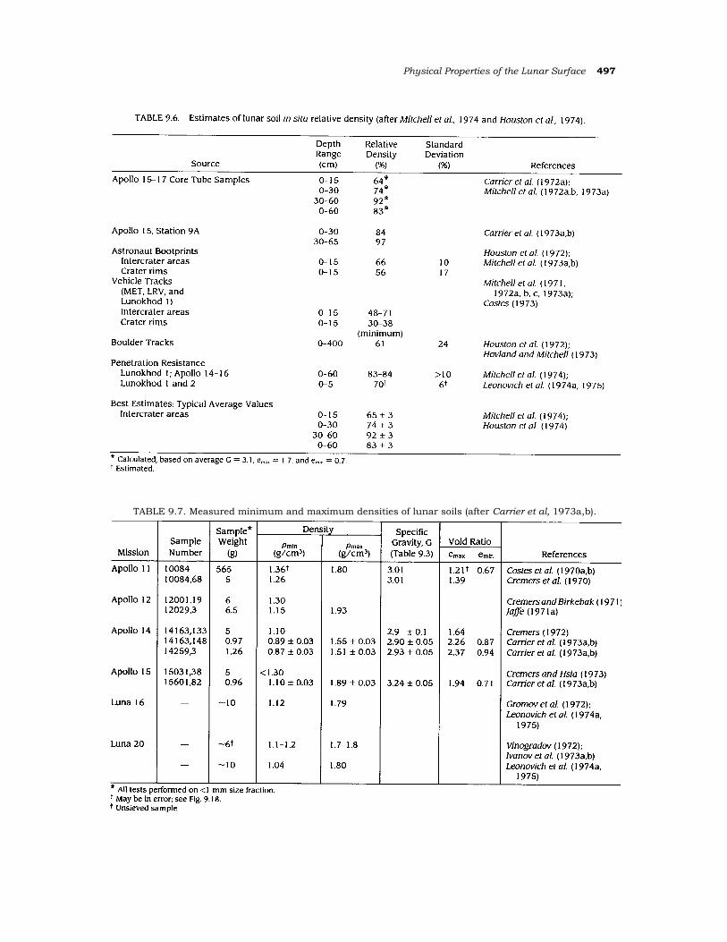
A summary of estimated lunar soil relative densities is presented in Table 9.6, together with typical average values. The various estimating and measuring techniques are described in the following sections.
Laboratory measurements of minimum and maximum density. Values for minimum and maximum density of lunar soils are presented in
Table 9.7. In those cases where the specific gravity is also known, the corresponding maximum and minimum void ratios have also been calculated.
The Apollo 11 minimum and maximum densities reported by Costes et al. (1970a,b) were determined as part of a study of penetration resistance. Cremers and his colleagues (Cremers, 1972; Cremers and Birkebak, 1971; Cremers and Hsia, 1973; Cremers et al., 1970) found only minimum densities for Apollo 11-15 samples as part of their investigation of thermal conductivity. The densities determined by Jaffe (1971a) were for a sample returned inside the scoop of the Surveyor 3 spacecraft and were part of a study on penetration resistance. Carrier et al. (1973a,b) made measurements of relative density on one Apollo 15 and two Apollo 14 samples. The densities of a Luna 16 sample were determined by Gromov et al. (1972) in connection with penetrometer, compressibility, and shear strength tests. Later, Leonovich et al. (1974a, 1975) also reported similar test results for samples from the Luna 16 and 20 missions.
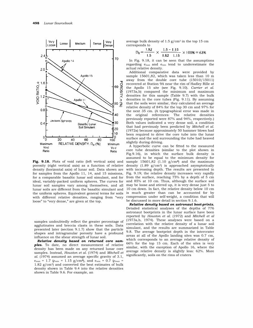
The maximum and minimum void ratios for the Apollo 11, 14, and 15 samples shown in Table 9.7 are plotted in Fig. 9.18. Also shown for comparison are the results for uniform spheres and for a basaltic simulant with a particle size distribution similar to that of the lunar soils. The minimum void ratio of the simulant is 0.45, corresponding to an intergranular porosity of 31%. However, the minimum void ratios of natural lunar soils are significantly higher. The value for the Apollo 15 sample is 0.71, or 0.26 greater than that of the simulant. This difference is a function of the intragranular void ratio, which represents approximately one-third of the total minimum void ratio of the Apollo 15 sample and corresponds to an intragranular porosity of about 21%.
Similar relations are seen in lunar soils from other missions. The minimum void ratio of the two Apollo 14 samples is approximately 0.46 greater than that of the simulant. This value represents approximately one-half of the total minimum void ratio of the Apollo 14 samples, corresponding to an intragranular porosity of about 32%. The intragranular porosity of the Apollo 11 sample appears to be similar to that of the Apollo 15 sample, but the slope of the line in Fig. 9.18 suggests that the maximum void ratio (minimum density) is in error.
Measurement of the minimum void ratio of a lunar soil can thus be used to estimate its intragranular porosity. The resulting porosity values of 21% to 32% are large compared to typical terrestrial granular soils, and this result is another indication of the significance of the irregular, reentrant shapes of lunar soil particles. The higher values for Apollo 14
Physical Properties of the Lunar Surface 497
TABLE 9.7. Measured minimum and maximum densities of lunar soils (after Carrier et al, 1973a,b).
498 Lunar Sourcebook
Fig. 9.18. Plots of void ratio (left vertical axis) and porosity (right vertical axis) as a function of relative density (horizontal axis) of lunar soil. Data shown are for samples from the Apollo 11, 14, and 15 missions, for a comparable basaltic lunar soil simulant, and for ideal, variably-packed uniform spheres. The curves for lunar soil samples vary among themselves, and all lunar soils are different from the basaltic simulant and the uniform spheres. Equivalent general terms for soils with different relative densities, ranging from “very loose” to “very dense,” are given at the top.
samples undoubtedly reflect the greater percentage of agglutinates and breccia clasts in these soils. Data presented later (section 9.1.7) show that the particle shapes and intragranular porosity have a profound influence on the shear strength of lunar soil.
Relative density based on returned core sam-ples. To date, no direct measurement of relative density has been made on any returned lunar core samples. Instead, Houston et al. (1974) and Mitchell et al. (1974) assumed an average specific gravity of 3.1, emax = 1.7 (ρmin = 1.15 g/cm3), and emin = 0.7 (ρmax = 1.82 g/cm3) and converted the best estimates of bulk density shown in Table 9.4 into the relative densities shown in Table 9.6. For example, an
average bulk density of 1.5 g/cm3 in the top 15 cm corresponds to
In Fig. 9.18, it can be seen that the assumptions
regarding emax and emin tend to underestimate the actual relative density.
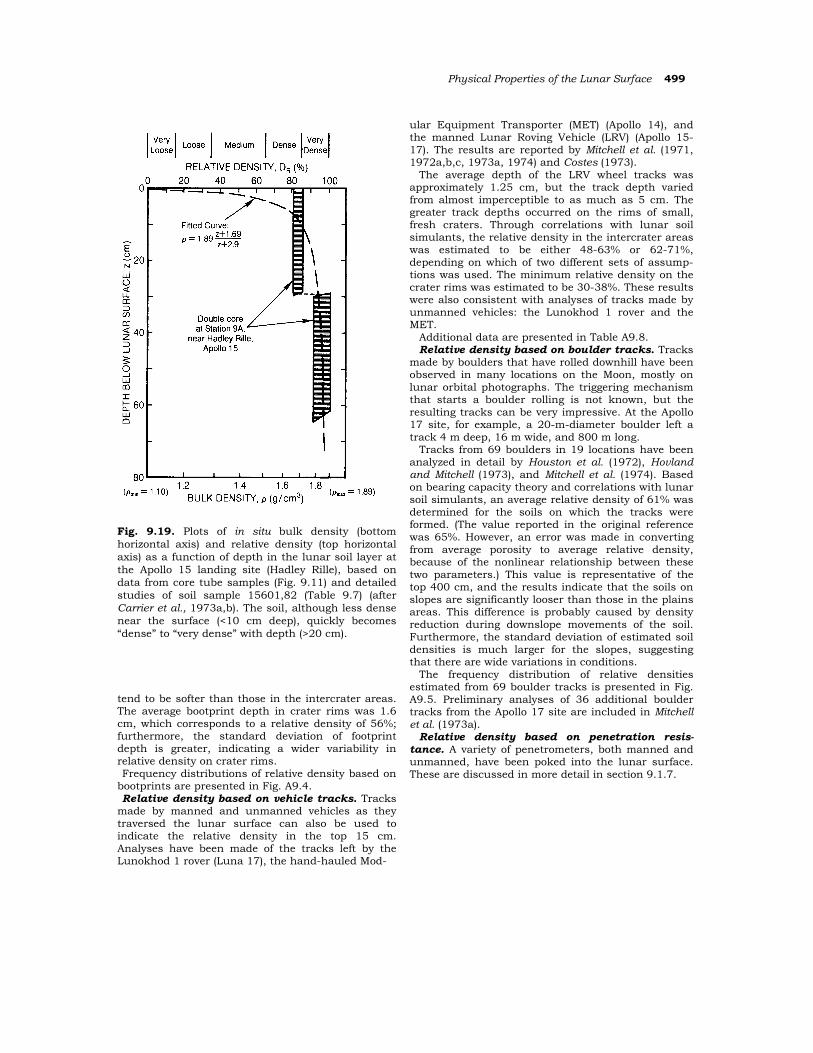
Additional comparative data were provided by sample 15601,82, which was taken less than 10 m away from the double core tube (15010/15011) recovered at Station 9A near the rim of Hadley Rille at the Apollo 15 site (see Fig. 9.10). Carrier et al. (1973a,b) compared the minimum and maximum densities for this sample (Table 9.7) with the bulk densities in the core tubes (Fig. 9.11). By assuming that the soils were similar, they calculated an average relative density of 84% for the top 30 cm and 97% for the next 35 cm. (A typographical error was made in the original references: The relative densities previously reported were 87% and 94%, respectively.) Both values indicated a very dense soil, a condition that had previously been predicted by Mitchell et al. (1972a) because approximately 50 hammer blows had been required to drive the core tube into the lunar surface and the soil surrounding the tube had heaved slightly during driving.
A hyperbolic curve can be fitted to the measured core tube densities (similar to the plot shown in Fig.9.16), in which the surface bulk density is assumed to be equal to the minimum density for sample 15601,82 (1.10 g/cm3) and the maximum density (1.89 g/cm3) is approached asymptotically with increasing depth. The results are presented in Fig. 9.19; the relative density increases very rapidly from the surface, reaching 75% by a depth of 5 cm and 85% at 10 cm. Thus, although the surface soil may be loose and stirred up, it is very dense just 5 to 10 cm down. In fact, the relative density below 10 cm is much greater than can be accounted for by compression under self-weight, a condition that will be discussed in more detail in section 9.1.6.
Relative density based on astronaut boot-prints. Detailed statistical analyses of the depths of 776 astronaut bootprints in the lunar surface have been reported by Houston et al. (1972) and Mitchell et al (1973a,b, 1974). These analyses were based on a correlation with the relative density of a lunar soil simulant, and the results are summarized in Table 9.8. The average bootprint depth in the intercrater areas at all of the Apollo landing sites was 0.7 cm, which corresponds to an average relative density of 66% for the top 15 cm. Each of the sites is very similar, with the exception of Apollo 16, where the average relative density is slightly less: 62%. More significantly, soils on the rims of craters
Physical Properties of the Lunar Surface 499
Fig. 9.19. Plots of in situ bulk density (bottom horizontal axis) and relative density (top horizontal axis) as a function of depth in the lunar soil layer at the Apollo 15 landing site (Hadley Rille), based on data from core tube samples (Fig. 9.11) and detailed studies of soil sample 15601,82 (Table 9.7) (after Carrier et al., 1973a,b). The soil, although less dense near the surface (<10 cm deep), quickly becomes “dense” to “very dense” with depth (>20 cm).
tend to be softer than those in the intercrater areas. The average bootprint depth in crater rims was 1.6 cm, which corresponds to a relative density of 56%; furthermore, the standard deviation of footprint depth is greater, indicating a wider variability in relative density on crater rims. Frequency distributions of relative density based on
bootprints are presented in Fig. A9.4. Relative density based on vehicle tracks. Tracks
made by manned and unmanned vehicles as they traversed the lunar surface can also be used to indicate the relative density in the top 15 cm. Analyses have been made of the tracks left by the Lunokhod 1 rover (Luna 17), the hand-hauled Mod-
ular Equipment Transporter (MET) (Apollo 14), and the manned Lunar Roving Vehicle (LRV) (Apollo 15-17). The results are reported by Mitchell et al. (1971, 1972a,b,c, 1973a, 1974) and Costes (1973).
The average depth of the LRV wheel tracks was approximately 1.25 cm, but the track depth varied from almost imperceptible to as much as 5 cm. The greater track depths occurred on the rims of small, fresh craters. Through correlations with lunar soil simulants, the relative density in the intercrater areas was estimated to be either 48-63% or 62-71%, depending on which of two different sets of assump-tions was used. The minimum relative density on the crater rims was estimated to be 30-38%. These results were also consistent with analyses of tracks made by unmanned vehicles: the Lunokhod 1 rover and the MET.
Additional data are presented in Table A9.8. Relative density based on boulder tracks. Tracks
made by boulders that have rolled downhill have been observed in many locations on the Moon, mostly on lunar orbital photographs. The triggering mechanism that starts a boulder rolling is not known, but the resulting tracks can be very impressive. At the Apollo 17 site, for example, a 20-m-diameter boulder left a track 4 m deep, 16 m wide, and 800 m long.
Tracks from 69 boulders in 19 locations have been analyzed in detail by Houston et al. (1972), Hovland and Mitchell (1973), and Mitchell et al. (1974). Based on bearing capacity theory and correlations with lunar soil simulants, an average relative density of 61% was determined for the soils on which the tracks were formed. (The value reported in the original reference was 65%. However, an error was made in converting from average porosity to average relative density, because of the nonlinear relationship between these two parameters.) This value is representative of the top 400 cm, and the results indicate that the soils on slopes are significantly looser than those in the plains areas. This difference is probably caused by density reduction during downslope movements of the soil. Furthermore, the standard deviation of estimated soil densities is much larger for the slopes, suggesting that there are wide variations in conditions.
The frequency distribution of relative densities estimated from 69 boulder tracks is presented in Fig. A9.5. Preliminary analyses of 36 additional boulder tracks from the Apollo 17 site are included in Mitchell et al. (1973a).
Relative density based on penetration resis-tance. A variety of penetrometers, both manned and unmanned, have been poked into the lunar surface. These are discussed in more detail in section 9.1.7.
500 Lunar Sourcebook
TABLE 9.8. Summary of statistical analyses of relative density based on astronaut bootprint depth (depth range 0-15 cm) (after Houston et al., 1972; Mitchell et al., 1973a,b, 1974).
Mitchell et al. (1974) compared measurements of penetration resistance on the Lunokhod 1 and Apollo 14-16 missions, using correlations with lunar soil simulants. From these measurements, they deduced relative densities that varied from 63% to 95%, with an average value of 83-84%.
Leonovich et al. (1974a, 1975) analyzed the results of approximately 1000 cone penetrometer tests made by Lunokhod 1 and 2. They also presented the results of penetration measurements made on lunar soil returned by the Luna 16 and 20 missions. By comparing these measurements with the estimated values of minimum and maximum density in Table 9.7, the average relative density is calculated to be 70%. (In section 9.1.7, a somewhat lower value of relative density is deduced, based on a different analysis of the same data.) This value is representative of the top 5 cm of the lunar surface, over a combined traverse distance of 47 km. The frequency distribution of relative density based on the cone penetrometer tests on the Lunokhod 1 and 2 missions is presented in Fig. A9.6.
Best estimates of relative density. The in situ relative density of lunar soil has been estimated by a variety of methods, as described in the preceding sections. Despite differences in the values obtained from different data and by different methods, the following trends are apparent: (1) The relative density of lunar soil tends to be low on the rims of fresh craters, on slopes, and virtually everywhere within the top few centimeters of the surface. (2) However, in intercrater areas, the relative density is exception-ally high at depths of only 5-10 cm. (Shortly after the Apollo 11 mission, astronaut Edwin Aldrin walked and ran on a simulated lunar surface at the Johnson Space Center in Houston. The test facility consisted of a circular sand track, approximately 15 cm deep, 1 m wide, and 30 m in diameter; a special marionette rig supported five-sixths of Aldrin’s weight, including his spacesuit. When asked how the test track
compared to the real lunar surface, Aldrin replied that the sand was too yielding. While walking on the Moon, he had noticed that although the lunar soil was soft at the surface, there was a firmer stratum at a shallow depth.)
This large and relatively sudden change in relative density with increasing depth has been attributed to the effects of continuing small meteoroid impacts, which evidently generate a loose, stirred-up surface but at the same time shake and densify the underlying soil (Carrier et al., 1973a,b).
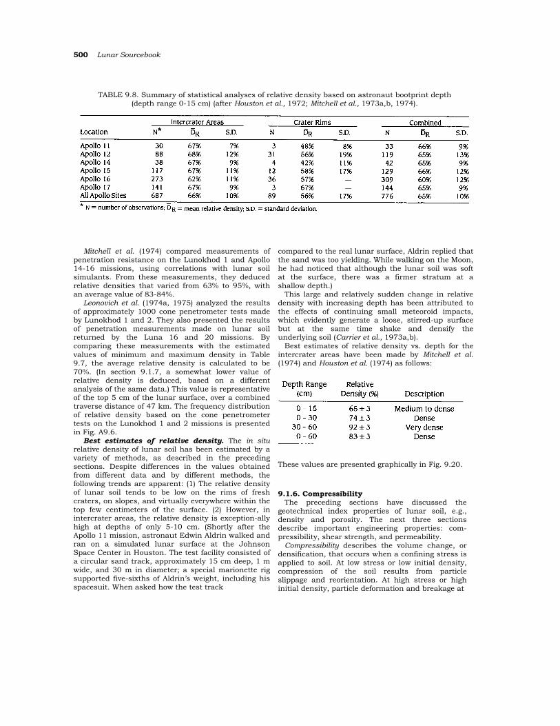
Best estimates of relative density vs. depth for the intercrater areas have been made by Mitchell et al. (1974) and Houston et al. (1974) as follows:
These values are presented graphically in Fig. 9.20.
9.1.6. Compressibility The preceding sections have discussed the
geotechnical index properties of lunar soil, e.g., density and porosity. The next three sections describe important engineering properties: com-pressibility, shear strength, and permeability.
Compressibility describes the volume change, or densification, that occurs when a confining stress is applied to soil. At low stress or low initial density, compression of the soil results from particle slippage and reorientation. At high stress or high initial density, particle deformation and breakage at
Physical Properties of the Lunar Surface 501
Fig. 9.20. Plot of typical average (“recommended”) values for relative density of lunar soils as a function of depth, using data collected from all Apollo missions (e.g., Fig. 9.19) (after Mitchell et al., 1974; Houston et al., 1974). With increasing depth, the lunar soil quickly becomes dense, reaching values of relative density equivalent to “dense” to “very dense” below about 20 cm.
the points of contact also occur. A summary of compressibility parameters is presented in Table 9.9 and discussed in the following sections.
Compression index. The compression index, Cc, is defined as the decrease in void ratio that occurs when the stress is increased by an order of magnitude
where ∆e = change in void ratio (negative) and ∆log σv = change in logarithm of applied vertical stress.
TABLE 9.9. Compressibility parameters of lunar soil.
To measure Cc in the laboratory, the soil is placed in a rigid ring at a known density (void ratio) and then squeezed with a vertical piston; this is called a one-dimensional oedometer test. The void ratio is plotted vs. the logarithm of applied stress and the slope of the curve yields the value of Cc.
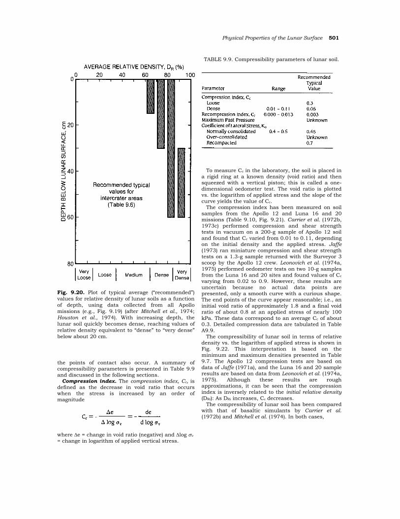
The compression index has been measured on soil samples from the Apollo 12 and Luna 16 and 20 missions (Table 9.10, Fig. 9.21). Carrier et al. (1972b, 1973c) performed compression and shear strength tests in vacuum on a 200-g sample of Apollo 12 soil and found that Cc varied from 0.01 to 0.11, depending on the initial density and the applied stress. Jaffe (1973) ran miniature compression and shear strength tests on a 1.3-g sample returned with the Surveyor 3 scoop by the Apollo 12 crew. Leonovich et al. (1974a, 1975) performed oedometer tests on two 10-g samples from the Luna 16 and 20 sites and found values of Cc varying from 0.02 to 0.9. However, these results are uncertain because no actual data points are presented, only a smooth curve with a curious shape. The end points of the curve appear reasonable; i.e., an initial void ratio of approximately 1.8 and a final void ratio of about 0.8 at an applied stress of nearly 100 kPa. These data correspond to an average Cc of about 0.3. Detailed compression data are tabulated in Table A9.9.
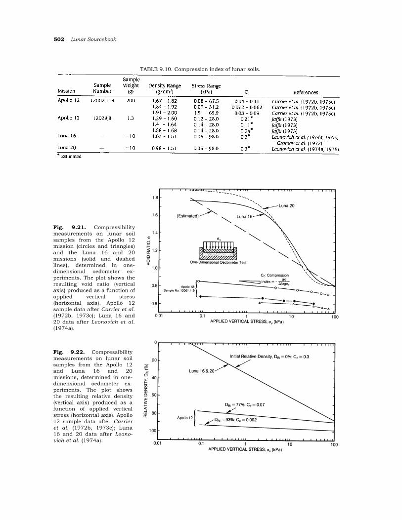
The compressibility of lunar soil in terms of relative density vs. the logarithm of applied stress is shown in Fig. 9.22. This interpretation is based on the minimum and maximum densities presented in Table 9.7. The Apollo 12 compression tests are based on data of Jaffe (1971a), and the Luna 16 and 20 sample results are based on data from Leonovich et al. (1974a, 1975). Although these results are rough approximations, it can be seen that the compression index is inversely related to the initial relative density (DRi): As DRi increases, Cc decreases.
The compressibility of lunar soil has been compared with that of basaltic simulants by Carrier et al. (1972b) and Mitchell et al. (1974). In both cases,
502 Lunar Sourcebook
TABLE 9.10. Compression index of lunar soils.
Fig. 9.21. Compressibilitymeasurements on lunar soilsamples from the Apollo 12mission (circles and triangles)and the Luna 16 and 20missions (solid and dashedlines), determined in one-dimensional oedometer ex-periments. The plot shows theresulting void ratio (verticalaxis) produced as a function ofapplied vertical stress(horizontal axis). Apollo 12sample data after Carrier et al.(1972b, 1973c); Luna 16 and20 data after Leonovich et al.(1974a).
Fig. 9.22. Compressibility measurements on lunar soil samples from the Apollo 12 and Luna 16 and 20 missions, determined in one-dimensional oedometer ex-periments. The plot shows the resulting relative density (vertical axis) produced as a function of applied vertical stress (horizontal axis). Apollo 12 sample data after Carrier et al. (1972b, 1973c); Luna 16 and 20 data after Leono-vich et al. (1974a).
Physical Properties of the Lunar Surface 503
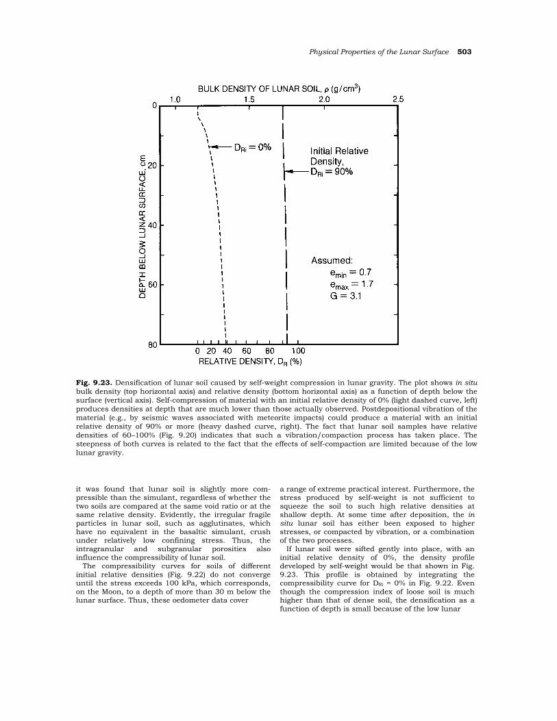
Fig. 9.23. Densification of lunar soil caused by self-weight compression in lunar gravity. The plot shows in situ bulk density (top horizontal axis) and relative density (bottom horizontal axis) as a function of depth below the surface (vertical axis). Self-compression of material with an initial relative density of 0% (light dashed curve, left) produces densities at depth that are much lower than those actually observed. Postdepositional vibration of the material (e.g., by seismic waves associated with meteorite impacts) could produce a material with an initial relative density of 90% or more (heavy dashed curve, right). The fact that lunar soil samples have relative densities of 60–100% (Fig. 9.20) indicates that such a vibration/compaction process has taken place. The steepness of both curves is related to the fact that the effects of self-compaction are limited because of the low lunar gravity.
it was found that lunar soil is slightly more com-pressible than the simulant, regardless of whether the two soils are compared at the same void ratio or at the same relative density. Evidently, the irregular fragile particles in lunar soil, such as agglutinates, which have no equivalent in the basaltic simulant, crush under relatively low confining stress. Thus, the intragranular and subgranular porosities also influence the compressibility of lunar soil.
The compressibility curves for soils of different initial relative densities (Fig. 9.22) do not converge until the stress exceeds 100 kPa, which corresponds, on the Moon, to a depth of more than 30 m below the lunar surface. Thus, these oedometer data cover
a range of extreme practical interest. Furthermore, the stress produced by self-weight is not sufficient to squeeze the soil to such high relative densities at shallow depth. At some time after deposition, the in situ lunar soil has either been exposed to higher stresses, or compacted by vibration, or a combination of the two processes.
If lunar soil were sifted gently into place, with an initial relative density of 0%, the density profile developed by self-weight would be that shown in Fig. 9.23. This profile is obtained by integrating the compressibility curve for DRi = 0% in Fig. 9.22. Even though the compression index of loose soil is much higher than that of dense soil, the densification as a function of depth is small because of the low lunar
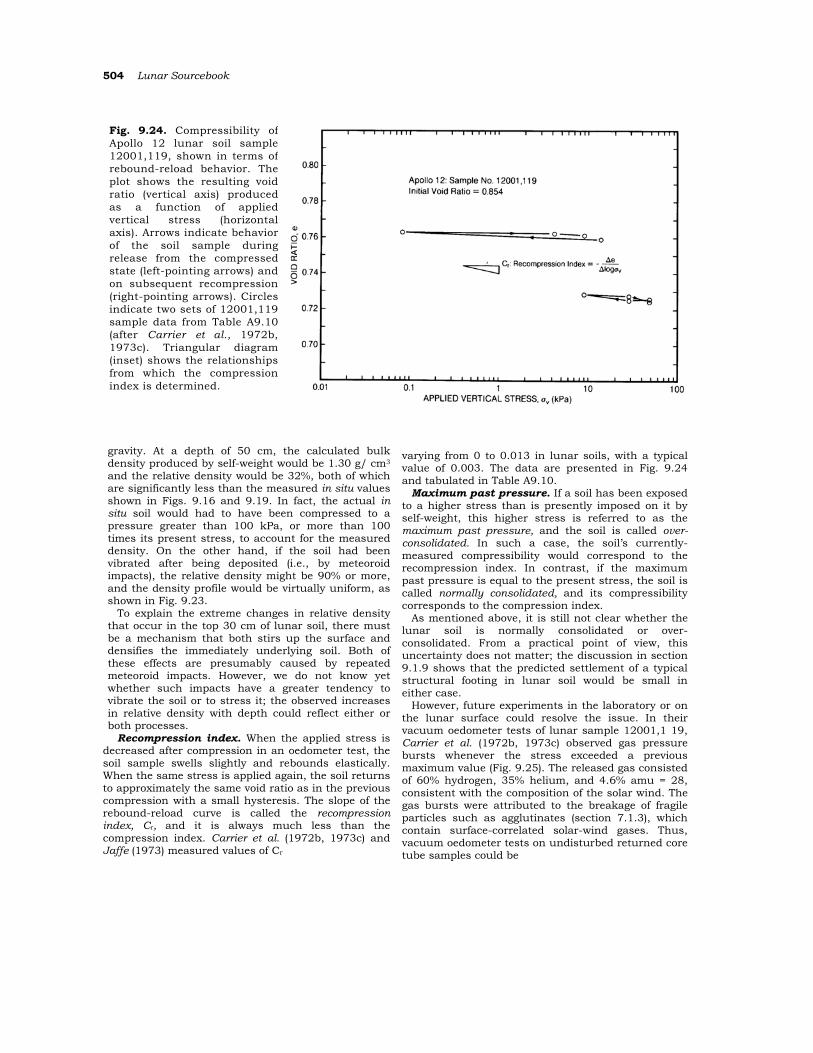
504 Lunar Sourcebook
gravity. At a depth of 50 cm, the calculated bulk density produced by self-weight would be 1.30 g/ cm3 and the relative density would be 32%, both of which are significantly less than the measured in situ values shown in Figs. 9.16 and 9.19. In fact, the actual in situ soil would had to have been compressed to a pressure greater than 100 kPa, or more than 100 times its present stress, to account for the measured density. On the other hand, if the soil had been vibrated after being deposited (i.e., by meteoroid impacts), the relative density might be 90% or more, and the density profile would be virtually uniform, as shown in Fig. 9.23.
To explain the extreme changes in relative density that occur in the top 30 cm of lunar soil, there must be a mechanism that both stirs up the surface and densifies the immediately underlying soil. Both of these effects are presumably caused by repeated meteoroid impacts. However, we do not know yet whether such impacts have a greater tendency to vibrate the soil or to stress it; the observed increases in relative density with depth could reflect either or both processes.
Recompression index. When the applied stress is decreased after compression in an oedometer test, the soil sample swells slightly and rebounds elastically. When the same stress is applied again, the soil returns to approximately the same void ratio as in the previous compression with a small hysteresis. The slope of the rebound-reload curve is called the recompression index, Cr, and it is always much less than the compression index. Carrier et al. (1972b, 1973c) and Jaffe (1973) measured values of Cr
varying from 0 to 0.013 in lunar soils, with a typical value of 0.003. The data are presented in Fig. 9.24 and tabulated in Table A9.10.
Maximum past pressure. If a soil has been exposed to a higher stress than is presently imposed on it by self-weight, this higher stress is referred to as the maximum past pressure, and the soil is called over-consolidated. In such a case, the soil’s currently-measured compressibility would correspond to the recompression index. In contrast, if the maximum past pressure is equal to the present stress, the soil is called normally consolidated, and its compressibility corresponds to the compression index.
As mentioned above, it is still not clear whether the lunar soil is normally consolidated or over-consolidated. From a practical point of view, this uncertainty does not matter; the discussion in section 9.1.9 shows that the predicted settlement of a typical structural footing in lunar soil would be small in either case.
However, future experiments in the laboratory or on the lunar surface could resolve the issue. In their vacuum oedometer tests of lunar sample 12001,1 19, Carrier et al. (1972b, 1973c) observed gas pressure bursts whenever the stress exceeded a previous maximum value (Fig. 9.25). The released gas consisted of 60% hydrogen, 35% helium, and 4.6% amu = 28, consistent with the composition of the solar wind. The gas bursts were attributed to the breakage of fragile particles such as agglutinates (section 7.1.3), which contain surface-correlated solar-wind gases. Thus, vacuum oedometer tests on undisturbed returned core tube samples could be
Fig. 9.24. Compressibility ofApollo 12 lunar soil sample12001,119, shown in terms ofrebound-reload behavior. Theplot shows the resulting voidratio (vertical axis) producedas a function of appliedvertical stress (horizontalaxis). Arrows indicate behaviorof the soil sample duringrelease from the compressedstate (left-pointing arrows) andon subsequent recompression(right-pointing arrows). Circlesindicate two sets of 12001,119sample data from Table A9.10(after Carrier et al., 1972b,1973c). Triangular diagram(inset) shows the relationshipsfrom which the compressionindex is determined.
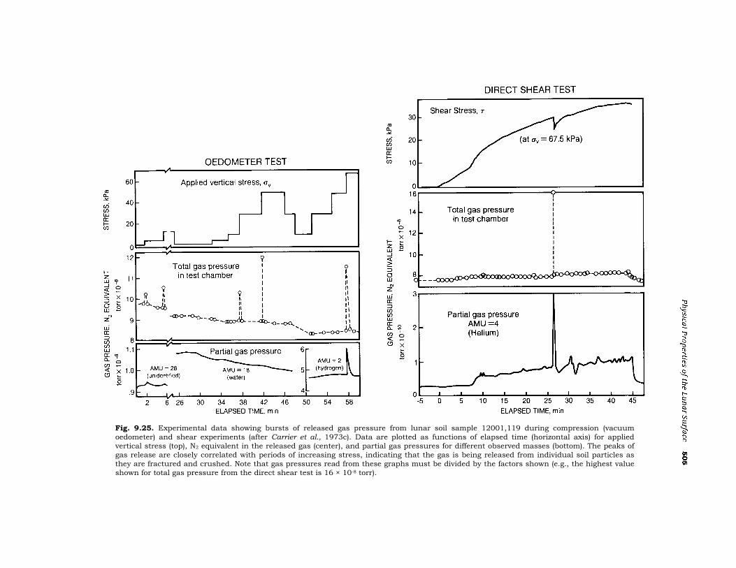
Fig. 9.25. Experimental data showing bursts of released gas pressure from lunar soil sample 12001,119 during compression (vacuum oedometer) and shear experiments (after Carrier et al., 1973c). Data are plotted as functions of elapsed time (horizontal axis) for applied vertical stress (top), N2 equivalent in the released gas (center), and partial gas pressures for different observed masses (bottom). The peaks of gas release are closely correlated with periods of increasing stress, indicating that the gas is being released from individual soil particles as they are fractured and crushed. Note that gas pressures read from these graphs must be divided by the factors shown (e.g., the highest value shown for total gas pressure from the direct shear test is 16 × 10-8 torr).
506 Lunar Sourcebook
used to measure maximum past pressure. Alterna-tively, loading tests on undisturbed soil could be performed in situ as part of future robotic or human missions to the Moon. Such studies would provide valuable information regarding the mechanics of regolith evolution and impact crater formation.
Coefficient of lateral stress. The coefficient of lateral stress, Ko, defines the ratio of horizontal stress, σh, to vertical stress, σv
No measurements of Ko have been made on lunar soils. But if the lunar soil is normally consolidated, Ko would be approximately 0.4 to 0.5. If the soil is over-consolidated, then Ko could be greater, depending on the ratio of the maximum past pressure to the present pressure. Below a depth of a few meters, the maximum possible value of Ko is probably 3-5. In the future, better estimates of the in situ Ko of lunar soils may be necessary for the design of tunnels in the lunar surface.
If the lunar soil were excavated and then recom-pacted against the wall of a structure, a design value of Ko = 0.7 is recommended, based on terrestrial construction experience.
9.1.7. Shear Strength
The shear strength of a granular soil is typically defined in terms of the classic Mohr-Coulomb equation
where τ = shear strength (kPa); σ = normal stress (kPa); c = cohesion (kPa); and φ = friction angle.
The shear strength therefore consists of two components: a cohesive component that is inde-pendent of the applied stress, and a frictional component that is directly proportional to the normal stress (i.e., the stress that is perpendicular to the failure surface).
The shear strength governs such important engineering properties as ultimate bearing capacity, slope stability, and trafficability. As a result, estimates of lunar soil cohesion and friction angle have been the object of intensive research, as summarized in Table 9.11. In retrospect, many of the early inferred values, and even some early estimates from the subsequent Surveyor landings, were wide of the mark. The best available estimates prior to the Apollo 11 mission (July 1969) were derived from the soil mechanics surface sampler on the Surveyor 3 and 7 spacecraft (Scott and Roberson, 1969):
We now know that the Surveyor Model values are near the lower bounds of actual lunar soil shear strength. Based on a variety of data sources, including the manned Apollo missions, Mitchell et al. (1972d, 1974) have developed the Apollo Model:
The higher shear strength parameters correspond
to higher values of relative density of the lunar soil. We have plotted all the estimates of cohesion and
friction angle made with data from the Apollo and Lunokhod missions in terms of shear strength vs. normal stress (Fig. 9.26). This figure also shows, for comparison, the shear strengths of a basaltic simulant at relative densities of 30% and 90%, which bracket the shear strengths of the in situ lunar soil. These latter curves are based on data from Mitchell et al. (1972d, 1974) (Fig. 9.27). All the variations in the estimates of cohesion and friction angle can be accounted for by differences in the in situ relative density.
The estimates and measurements underlying these results are described in the following sections. Recommended typical values are summarized in Table 9.12.
Apollo 11 and 12 measurements. The estimates of shear strength made from observations at the Apollo 11 and 12 sites were limited to analyses of physical interactions with the lunar surface, including the Lunar Module (LM) landing; astronauts walking on level ground and on crater slopes; and penetration into the soil by core tubes, the flag pole, and the Solar Wind Composition (SWC) shaft. Although crude, these estimates showed that the lunar surface was at least as strong as predicted by the Surveyor Model (Costes et al., 1969).
Lunokhod 1. The first unmanned lunar rover, Lunokhod 1, was equipped with a cone penetrometer and a vane shear device. A total of 327 tests were performed in the lunar soil to depths of 10 cm along a 5-km traverse in the western part of Mare Imbrium. More details are given immediately below.
Apollo 14. Two experiments on the Apollo 14 mission were conducted specifically to evaluate the shear strength properties of lunar soils: (1) The astronauts excavated a shallow trench, and (2) they pushed a rod into the surface. The latter was called the Apollo Simple Penetrometer (ASP) because it had
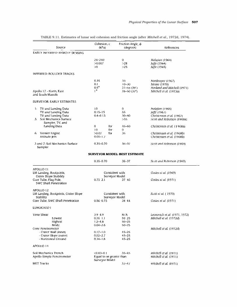
Physical Properties of the Lunar Surface 507
TABLE 9.11. Estimates of lunar soil cohesion and friction angle (after Mitchell et al., 1972d, 1974).
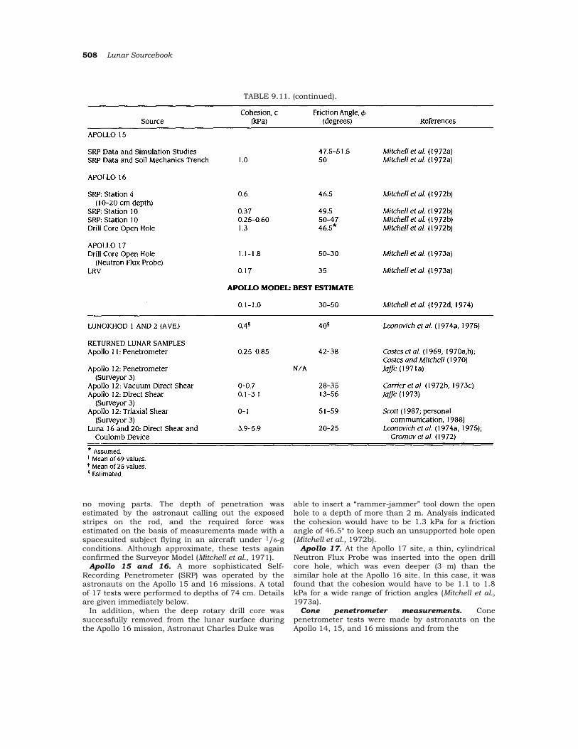
508 Lunar Sourcebook
TABLE 9.11. (continued).
no moving parts. The depth of penetration was estimated by the astronaut calling out the exposed stripes on the rod, and the required force was estimated on the basis of measurements made with a spacesuited subject flying in an aircraft under 1/6-g conditions. Although approximate, these tests again confirmed the Surveyor Model (Mitchell et al., 1971).
Apollo 15 and 16. A more sophisticated Self-Recording Penetrometer (SRP) was operated by the astronauts on the Apollo 15 and 16 missions. A total of 17 tests were performed to depths of 74 cm. Details are given immediately below.
In addition, when the deep rotary drill core was successfully removed from the lunar surface during the Apollo 16 mission, Astronaut Charles Duke was
able to insert a “rammer-jammer” tool down the open hole to a depth of more than 2 m. Analysis indicated the cohesion would have to be 1.3 kPa for a friction angle of 46.5° to keep such an unsupported hole open (Mitchell et al., 1972b).
Apollo 17. At the Apollo 17 site, a thin, cylindrical Neutron Flux Probe was inserted into the open drill core hole, which was even deeper (3 m) than the similar hole at the Apollo 16 site. In this case, it was found that the cohesion would have to be 1.1 to 1.8 kPa for a wide range of friction angles (Mitchell et al., 1973a).
Cone penetrometer measurements. Cone penetrometer tests were made by astronauts on the Apollo 14, 15, and 16 missions and from the
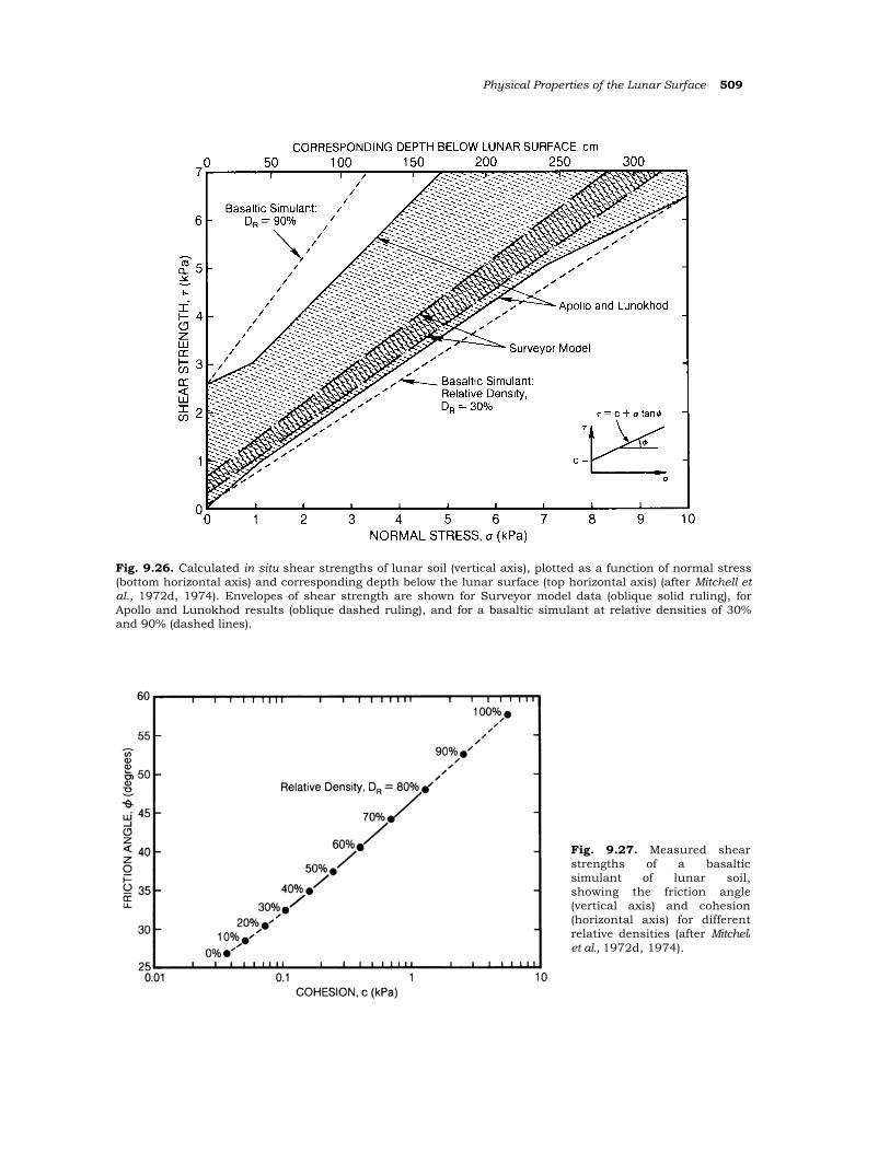
Physical Properties of the Lunar Surface 509
Fig. 9.26. Calculated in situ shear strengths of lunar soil (vertical axis), plotted as a function of normal stress (bottom horizontal axis) and corresponding depth below the lunar surface (top horizontal axis) (after Mitchell et al., 1972d, 1974). Envelopes of shear strength are shown for Surveyor model data (oblique solid ruling), for Apollo and Lunokhod results (oblique dashed ruling), and for a basaltic simulant at relative densities of 30% and 90% (dashed lines).
Fig. 9.27. Measured shearstrengths of a basalticsimulant of lunar soil,showing the friction angle(vertical axis) and cohesion(horizontal axis) for differentrelative densities (after Mitchellet al., 1972d, 1974).
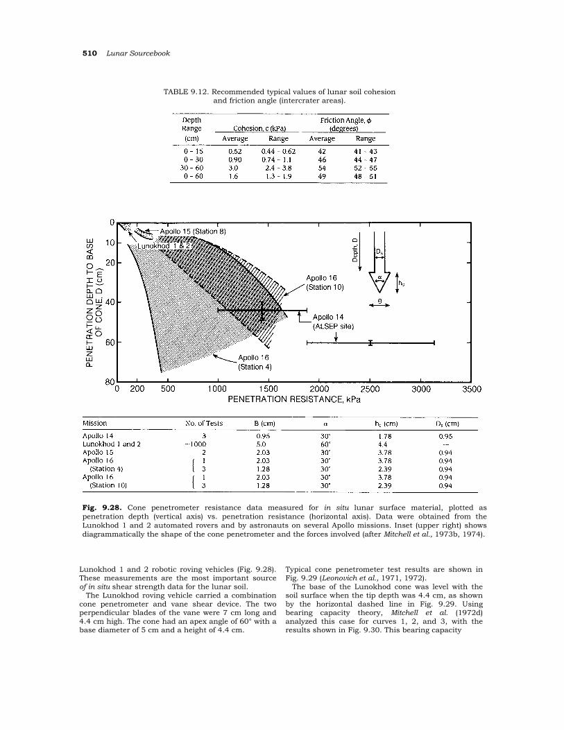
510 Lunar Sourcebook
TABLE 9.12. Recommended typical values of lunar soil cohesion and friction angle (intercrater areas).
Fig. 9.28. Cone penetrometer resistance data measured for in situ lunar surface material, plotted as penetration depth (vertical axis) vs. penetration resistance (horizontal axis). Data were obtained from the Lunokhod 1 and 2 automated rovers and by astronauts on several Apollo missions. Inset (upper right) shows diagrammatically the shape of the cone penetrometer and the forces involved (after Mitchell et al., 1973b, 1974).
Lunokhod 1 and 2 robotic roving vehicles (Fig. 9.28). These measurements are the most important source of in situ shear strength data for the lunar soil.
The Lunokhod roving vehicle carried a combination cone penetrometer and vane shear device. The two perpendicular blades of the vane were 7 cm long and 4.4 cm high. The cone had an apex angle of 60° with a base diameter of 5 cm and a height of 4.4 cm.
Typical cone penetrometer test results are shown in Fig. 9.29 (Leonovich et al., 1971, 1972).
The base of the Lunokhod cone was level with the soil surface when the tip depth was 4.4 cm, as shown by the horizontal dashed line in Fig. 9.29. Using bearing capacity theory, Mitchell et al. (1972d) analyzed this case for curves 1, 2, and 3, with the results shown in Fig. 9.30. This bearing capacity
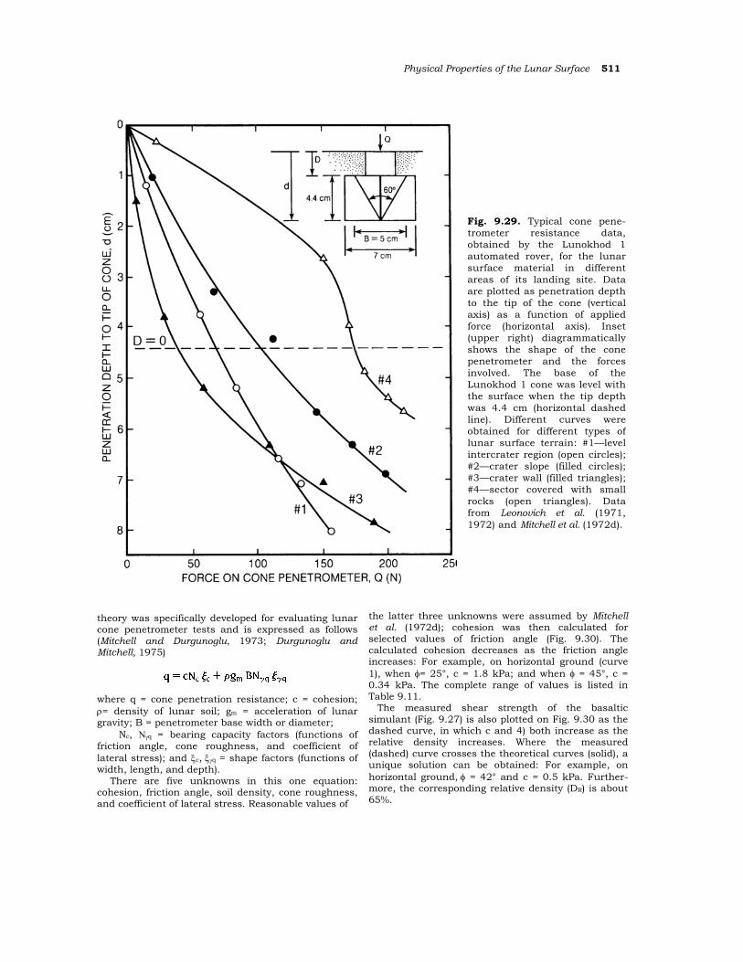
Physical Properties of the Lunar Surface 511
theory was specifically developed for evaluating lunar cone penetrometer tests and is expressed as follows (Mitchell and Durgunoglu, 1973; Durgunoglu and Mitchell, 1975)
where q = cone penetration resistance; c = cohesion; ρ= density of lunar soil; gm = acceleration of lunar gravity; B = penetrometer base width or diameter;
Nc, Νγq = bearing capacity factors (functions of friction angle, cone roughness, and coefficient of lateral stress); and ξc, ξγq = shape factors (functions of width, length, and depth).
There are five unknowns in this one equation: cohesion, friction angle, soil density, cone roughness, and coefficient of lateral stress. Reasonable values of
the latter three unknowns were assumed by Mitchell et al. (1972d); cohesion was then calculated for selected values of friction angle (Fig. 9.30). The calculated cohesion decreases as the friction angle increases: For example, on horizontal ground (curve 1), when φ= 25°, c = 1.8 kPa; and when φ = 45°, c = 0.34 kPa. The complete range of values is listed in Table 9.11.
The measured shear strength of the basaltic simulant (Fig. 9.27) is also plotted on Fig. 9.30 as the dashed curve, in which c and 4) both increase as the relative density increases. Where the measured (dashed) curve crosses the theoretical curves (solid), a unique solution can be obtained: For example, on horizontal ground, φ = 42° and c = 0.5 kPa. Further-more, the corresponding relative density (DR) is about 65%.
Fig. 9.29. Typical cone pene-trometer resistance data,obtained by the Lunokhod 1automated rover, for the lunarsurface material in differentareas of its landing site. Dataare plotted as penetration depthto the tip of the cone (verticalaxis) as a function of appliedforce (horizontal axis). Inset(upper right) diagrammaticallyshows the shape of the conepenetrometer and the forcesinvolved. The base of theLunokhod 1 cone was level withthe surface when the tip depthwas 4.4 cm (horizontal dashedline). Different curves wereobtained for different types oflunar surface terrain: #1—levelintercrater region (open circles);#2—crater slope (filled circles);#3—crater wall (filled triangles);#4—sector covered with smallrocks (open triangles). Datafrom Leonovich et al. (1971,1972) and Mitchell et al. (1972d).
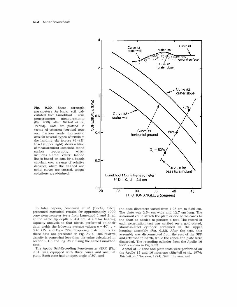
512 Lunar Sourcebook
In later papers, Leonovich et al. (1974a, 1975) presented statistical results for approximately 1000 cone penetrometer tests from Lunokhod 1 and 2, all at the same tip depth of 4.4 cm. A similar bearing capacity analysis to that above, performed on their data, yields the following average values: φ = 40°, c = 0.40 kPa, and DR = 59%. Frequency distributions for these data are presented in Fig. A9.7. This relative density is somewhat less than the value calculated in section 9.1.5 and Fig. A9.6 using the same Lunokhod data.
The Apollo Self-Recording Penetrometer (SRP) (Fig. 9.31) was equipped with three cones and one flat plate. Each cone had an apex angle of 30°, and
the base diameters varied from 1.28 cm to 2.86 cm. The plate was 2.54 cm wide and 12.7 cm long. The astronaut could attach the plate or one of the cones to the shaft as needed to perform a test. The record of each penetration test was scribed on a gold-plated, stainless-steel cylinder contained in the upper housing assembly (Fig. 9.32). After the test, this assembly was disconnected from the rest of the SRP and returned to Earth, while the cones and plate were discarded. The recording cylinder from the Apollo 16 SRP is shown in Fig. 9.33.
A total of 17 cone and plate tests were performed on the Apollo 15 and 16 missions (Mitchell et al., 1974; Mitchell and Houston, 1974). With the smallest
Fig. 9.30. Shear strengthparameters for lunar soil, cal-culated from Lunokhod 1 conepenetrometer measurements(Fig. 9.29) (after Mitchell et al.,1972d). Data are plotted interms of cohesion (vertical axis)and friction angle (horizontalaxis) for several types of terrain atthe landing site (curves #1–#3).Inset (upper right) shows relationof measurement locations to thesurface topography, whichincludes a small crater. Dashedline is based on data for a basaltsimulant over a range of relativedensities; where the dashed andsolid curves are crossed, uniquesolutions are obtained.
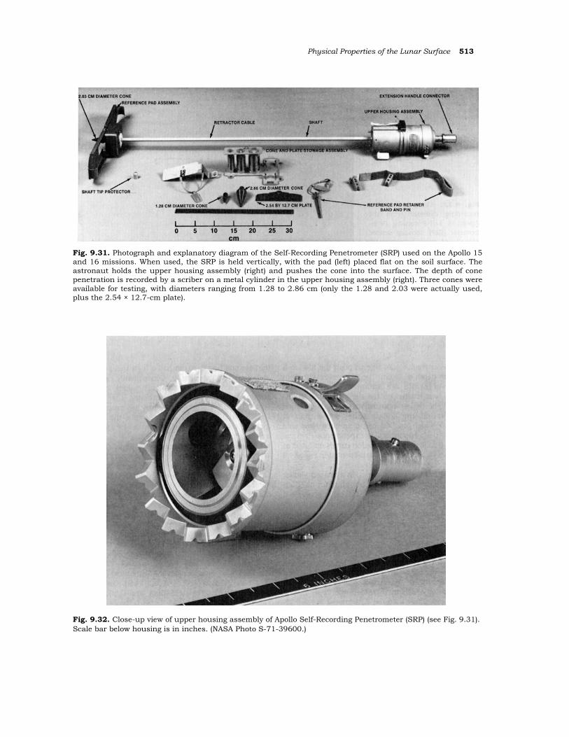
Physical Properties of the Lunar Surface 513
Fig. 9.31. Photograph and explanatory diagram of the Self-Recording Penetrometer (SRP) used on the Apollo 15 and 16 missions. When used, the SRP is held vertically, with the pad (left) placed flat on the soil surface. The astronaut holds the upper housing assembly (right) and pushes the cone into the surface. The depth of cone penetration is recorded by a scriber on a metal cylinder in the upper housing assembly (right). Three cones were available for testing, with diameters ranging from 1.28 to 2.86 cm (only the 1.28 and 2.03 were actually used, plus the 2.54 × 12.7-cm plate).
Fig. 9.32. Close-up view of upper housing assembly of Apollo Self-Recording Penetrometer (SRP) (see Fig. 9.31). Scale bar below housing is in inches. (NASA Photo S-71-39600.)
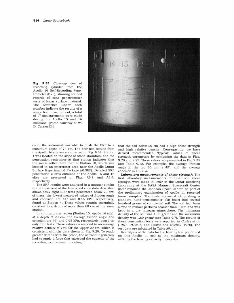
514 Lunar Sourcebook
Fig. 9.33. Close-up view of recording cylinder from the Apollo 16 Self-Recording Pene-trometer (SRP), showing scribed records of cone penetrometer tests of lunar surface material. The scratches under each number indicate the results of a single test measurement; a total of 17 measurements were made during the Apollo 15 and 16 missions. (Photo courtesy of W. D. Carrier III.)
cone, the astronaut was able to push the SRP to a maximum depth of 74 cm. The SRP test results from the Apollo 16 site are summarized in Fig. 9.34. Station 4 was located on the slope of Stone Mountain, and the penetration resistance at that station indicates that the soil is softer there than at Station 10, which was located in an intercrater area near the Apollo Lunar Surface Experimental Package (ALSEP). Detailed SRP penetration curves obtained at the Apollo 15 and 16 sites are presented in Figs. A9.8 and A9.9, respectively.
The SRP results were analyzed in a manner similar to the treatment of the Lunokhod cone data described above. Only eight SRP tests penetrated below 20 cm; of these, the lowest measured values of friction angle and cohesion are 41° and 0.45 kPa, respectively, found at Station 4. These values remain essentially constant to a depth of more than 60 cm at the same station.
In an intercrater region (Station 10, Apollo 16 site), at a depth of 20 cm, the average friction angle and cohesion are 46° and 0.95 kPa, respectively, based on only four tests. These values correspond to an average relative density of 75% for the upper 20 cm, which is consistent with the data shown in Fig. 9.20. To reach greater depths with the probe, the astronaut generally had to apply a force that exceeded the capacity of the recording mechanism, indicating
that the soil below 20 cm had a high shear strength and high relative density. Consequently, we have derived recommended “typical” values of shear strength parameters by combining the data in Figs. 9.20 and 9.27. These values are presented in Fig. 9.35 and Table 9.12. For example, the average friction angle in the top 60 cm is 49°, and the average cohesion is 1.6 kPa.
Laboratory measurements of shear strength. The first laboratory measurements of lunar soil shear strength were made in 1969 in the Lunar Receiving Laboratory at the NASA Manned Spacecraft Center (later renamed the Johnson Space Center) as part of the preliminary examination of Apollo 11 returned lunar samples. The tests consisted of pushing a standard hand-penetrometer (flat base) into several hundred grams of compacted soil. The soil had been sieved to remove particles coarser than 1 mm and was kept in a dry nitrogen atmosphere. The minimum density of the soil was 1.36 g/cm3 and the maximum density was 1.80 g/cm3 (see Table 9.7). The results of these penetration tests were reported in Costes et al. (1969, 1970a,b) and Costes and Mitchell (1970). The test data are tabulated in Table A9.1 1.
Reanalysis of the data for the bearing test performed on this Apollo 11 soil at the maximum density, utilizing the bearing capacity theory de-
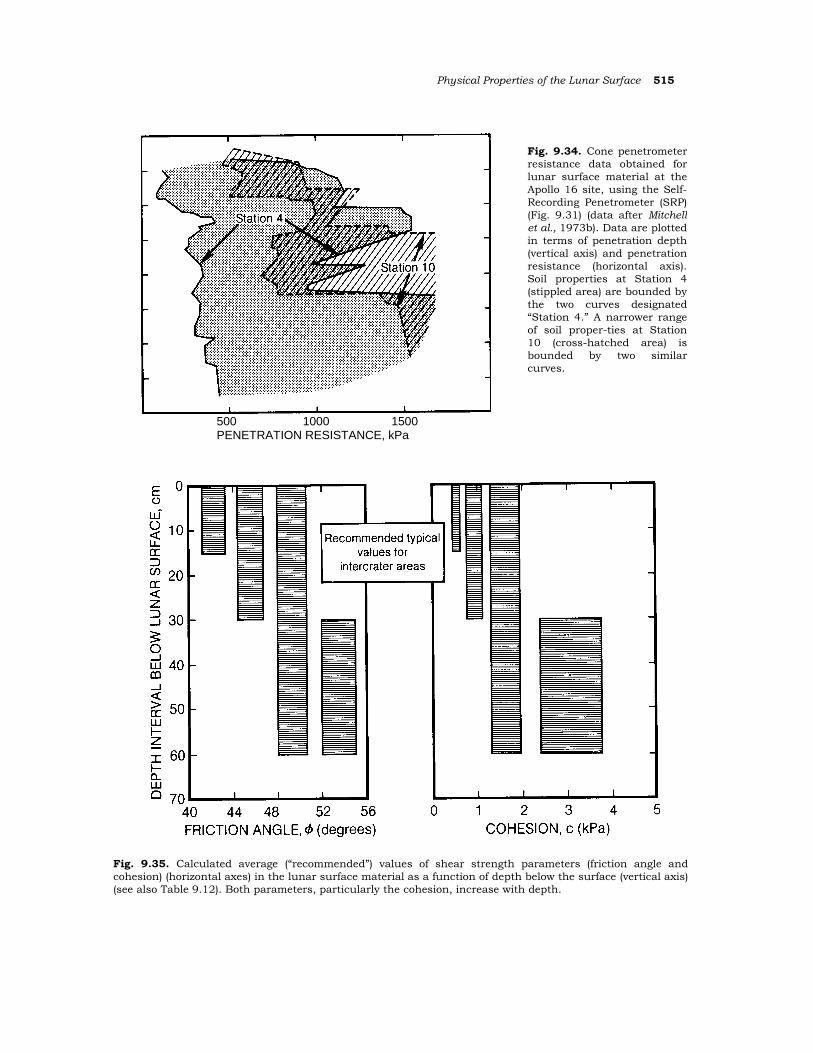
Physical Properties of the Lunar Surface 515
Fig. 9.35. Calculated average (“recommended”) values of shear strength parameters (friction angle and cohesion) (horizontal axes) in the lunar surface material as a function of depth below the surface (vertical axis) (see also Table 9.12). Both parameters, particularly the cohesion, increase with depth.
500 1000 1500 PENETRATION RESISTANCE, kPa
Fig. 9.34. Cone penetrometerresistance data obtained forlunar surface material at theApollo 16 site, using the Self-Recording Penetrometer (SRP)(Fig. 9.31) (data after Mitchellet al., 1973b). Data are plottedin terms of penetration depth(vertical axis) and penetrationresistance (horizontal axis).Soil properties at Station 4(stippled area) are bounded bythe two curves designated“Station 4.” A narrower rangeof soil proper-ties at Station10 (cross-hatched area) isbounded by two similarcurves.
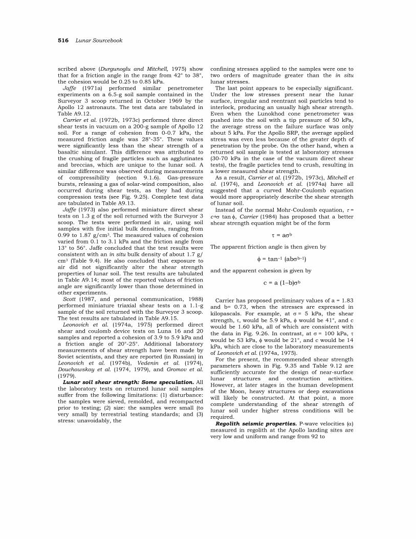
516 Lunar Sourcebook
scribed above (Durgunoglu and Mitchell, 1975) show that for a friction angle in the range from 42° to 38°, the cohesion would be 0.25 to 0.85 kPa.
Jaffe (1971a) performed similar penetrometer experiments on a 6.5-g soil sample contained in the Surveyor 3 scoop returned in October 1969 by the Apollo 12 astronauts. The test data are tabulated in Table A9.12.
Carrier et al. (1972b, 1973c) performed three direct shear tests in vacuum on a 200-g sample of Apollo 12 soil. For a range of cohesion from 0-0.7 kPa, the measured friction angle was 28°-35°. These values were significantly less than the shear strength of a basaltic simulant. This difference was attributed to the crushing of fragile particles such as agglutinates and breccias, which are unique to the lunar soil. A similar difference was observed during measurements of compressibility (section 9.1.6). Gas-pressure bursts, releasing a gas of solar-wind composition, also occurred during shear tests, as they had during compression tests (see Fig. 9.25). Complete test data are tabulated in Table A9.13.
Jaffe (1973) also performed miniature direct shear tests on 1.3 g of the soil returned with the Surveyor 3 scoop. The tests were performed in air, using soil samples with five initial bulk densities, ranging from 0.99 to 1.87 g/cm3. The measured values of cohesion varied from 0.1 to 3.1 kPa and the friction angle from 13° to 56°. Jaffe concluded that the test results were consistent with an in situ bulk density of about 1.7 g/ cm3 (Table 9.4). He also concluded that exposure to air did not significantly alter the shear strength properties of lunar soil. The test results are tabulated in Table A9.14; most of the reported values of friction angle are significantly lower than those determined in other experiments.
Scott (1987, and personal communication, 1988) performed miniature triaxial shear tests on a 1.1-g sample of the soil returned with the Surveyor 3 scoop. The test results are tabulated in Table A9.15.
Leonovich et al. (1974a, 1975) performed direct shear and coulomb device tests on Luna 16 and 20 samples and reported a cohesion of 3.9 to 5.9 kPa and a friction angle of 20°-25°. Additional laboratory measurements of shear strength have been made by Soviet scientists, and they are reported (in Russian) in Leonovich et al. (1974b), Vedenin et al. (1974), Douchowskoy et al. (1974, 1979), and Gromov et al. (1979).
Lunar soil shear strength: Some speculation. All the laboratory tests on returned lunar soil samples suffer from the following limitations: (1) disturbance: the samples were sieved, remolded, and recompacted prior to testing; (2) size: the samples were small (to very small) by terrestrial testing standards; and (3) stress: unavoidably, the
confining stresses applied to the samples were one to two orders of magnitude greater than the in situ lunar stresses.
The last point appears to be especially significant. Under the low stresses present near the lunar surface, irregular and reentrant soil particles tend to interlock, producing an usually high shear strength. Even when the Lunokhod cone penetrometer was pushed into the soil with a tip pressure of 50 kPa, the average stress on the failure surface was only about 5 kPa. For the Apollo SRP, the average applied stress was even less because of the greater depth of penetration by the probe. On the other hand, when a returned soil sample is tested at laboratory stresses (30-70 kPa in the case of the vacuum direct shear tests), the fragile particles tend to crush, resulting in a lower measured shear strength.
As a result, Carrier et al. (1972b, 1973c), Mitchell et al. (1974), and Leonovich et al. (1974a) have all suggested that a curved Mohr-Coulomb equation would more appropriately describe the shear strength of lunar soil.
Instead of the normal Mohr-Coulomb equation, τ = c+σ tan φ, Carrier (1984) has proposed that a better shear strength equation might be of the form
τ = aσb
The apparent friction angle is then given by
φ = tan–1 (abσb–1)
and the apparent cohesion is given by
c = a (1–b)σb
Carrier has proposed preliminary values of a = 1.83 and b= 0.73, when the stresses are expressed in kilopascals. For example, at σ = 5 kPa, the shear strength, τ, would be 5.9 kPa, φ would be 41°, and c would be 1.60 kPa, all of which are consistent with the data in Fig. 9.26. In contrast, at σ = 100 kPa, τ would be 53 kPa, φ would be 21°, and c would be 14 kPa, which are close to the laboratory measurements of Leonovich et al. (1974a, 1975).
For the present, the recommended shear strength parameters shown in Fig. 9.35 and Table 9.12 are sufficiently accurate for the design of near-surface lunar structures and construction activities. However, at later stages in the human development of the Moon, heavy structures or deep excavations will likely be constructed. At that point, a more complete understanding of the shear strength of lunar soil under higher stress conditions will be required.
Regolith seismic properties. P-wave velocities (α) measured in regolith at the Apollo landing sites are very low and uniform and range from 92 to
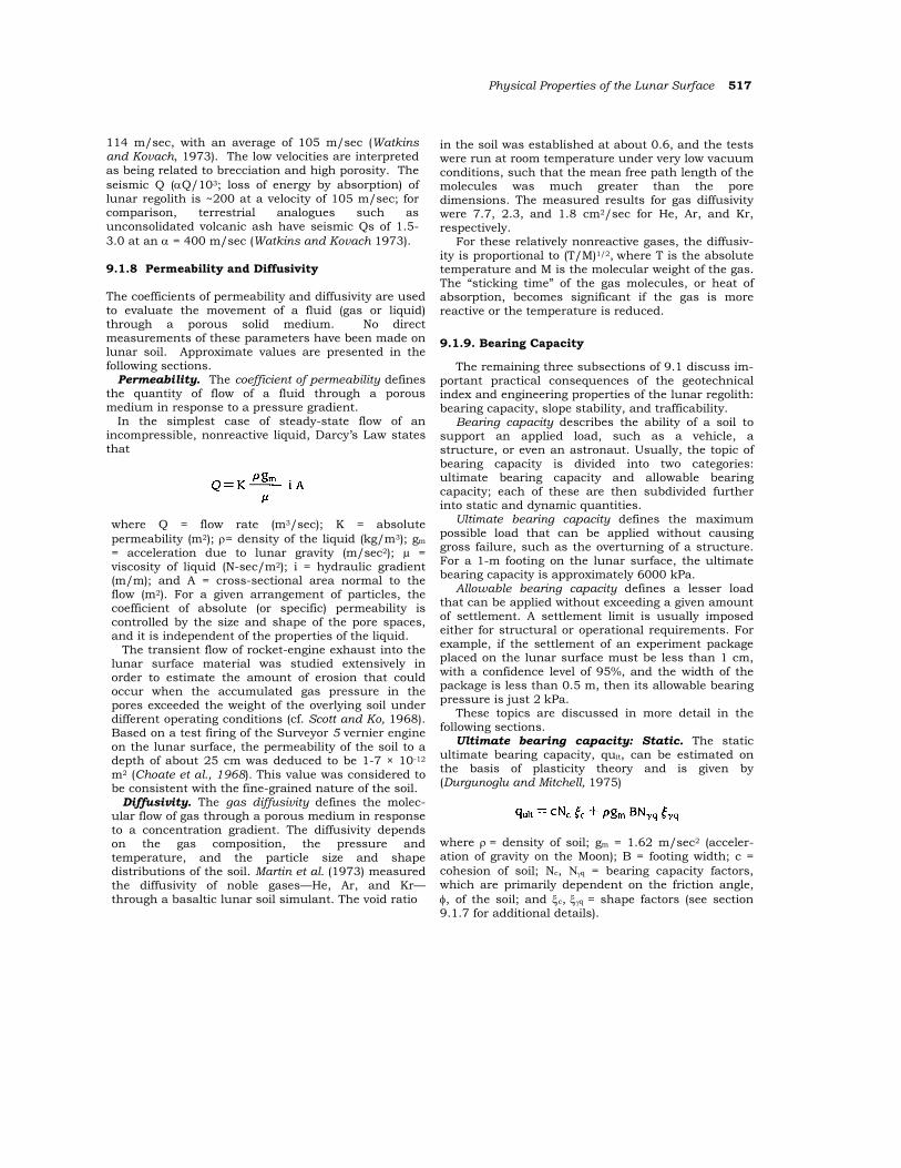
Physical Properties of the Lunar Surface 517
114 m/sec, with an average of 105 m/sec (Watkins and Kovach, 1973). The low velocities are interpreted as being related to brecciation and high porosity. The seismic Q (αQ/103; loss of energy by absorption) of lunar regolith is ~200 at a velocity of 105 m/sec; for comparison, terrestrial analogues such as unconsolidated volcanic ash have seismic Qs of 1.5-3.0 at an α = 400 m/sec (Watkins and Kovach 1973). 9.1.8 Permeability and Diffusivity The coefficients of permeability and diffusivity are used to evaluate the movement of a fluid (gas or liquid) through a porous solid medium. No direct measurements of these parameters have been made on lunar soil. Approximate values are presented in the following sections. Permeability. The coefficient of permeability defines the quantity of flow of a fluid through a porous medium in response to a pressure gradient. In the simplest case of steady-state flow of an incompressible, nonreactive liquid, Darcy’s Law states that
where Q = flow rate (m3/sec); K = absolute permeability (m2); ρ= density of the liquid (kg/m3); gm = acceleration due to lunar gravity (m/sec2); µ = viscosity of liquid (N-sec/m2); i = hydraulic gradient (m/m); and A = cross-sectional area normal to the flow (m2). For a given arrangement of particles, the coefficient of absolute (or specific) permeability is controlled by the size and shape of the pore spaces, and it is independent of the properties of the liquid.
The transient flow of rocket-engine exhaust into the lunar surface material was studied extensively in order to estimate the amount of erosion that could occur when the accumulated gas pressure in the pores exceeded the weight of the overlying soil under different operating conditions (cf. Scott and Ko, 1968). Based on a test firing of the Surveyor 5 vernier engine on the lunar surface, the permeability of the soil to a depth of about 25 cm was deduced to be 1-7 × 10-12
m2 (Choate et al., 1968). This value was considered to be consistent with the fine-grained nature of the soil.
Diffusivity. The gas diffusivity defines the molec-ular flow of gas through a porous medium in response to a concentration gradient. The diffusivity depends on the gas composition, the pressure and temperature, and the particle size and shape distributions of the soil. Martin et al. (1973) measured the diffusivity of noble gases—He, Ar, and Kr—through a basaltic lunar soil simulant. The void ratio
in the soil was established at about 0.6, and the tests were run at room temperature under very low vacuum conditions, such that the mean free path length of the molecules was much greater than the pore dimensions. The measured results for gas diffusivity were 7.7, 2.3, and 1.8 cm2/sec for He, Ar, and Kr, respectively.
For these relatively nonreactive gases, the diffusiv-ity is proportional to (T/M)1/2, where T is the absolute temperature and M is the molecular weight of the gas. The “sticking time” of the gas molecules, or heat of absorption, becomes significant if the gas is more reactive or the temperature is reduced.
9.1.9. Bearing Capacity
The remaining three subsections of 9.1 discuss im-portant practical consequences of the geotechnical index and engineering properties of the lunar regolith: bearing capacity, slope stability, and trafficability.
Bearing capacity describes the ability of a soil to support an applied load, such as a vehicle, a structure, or even an astronaut. Usually, the topic of bearing capacity is divided into two categories: ultimate bearing capacity and allowable bearing capacity; each of these are then subdivided further into static and dynamic quantities.
Ultimate bearing capacity defines the maximum possible load that can be applied without causing gross failure, such as the overturning of a structure. For a 1-m footing on the lunar surface, the ultimate bearing capacity is approximately 6000 kPa.
Allowable bearing capacity defines a lesser load that can be applied without exceeding a given amount of settlement. A settlement limit is usually imposed either for structural or operational requirements. For example, if the settlement of an experiment package placed on the lunar surface must be less than 1 cm, with a confidence level of 95%, and the width of the package is less than 0.5 m, then its allowable bearing pressure is just 2 kPa.
These topics are discussed in more detail in the following sections.
Ultimate bearing capacity: Static. The static ultimate bearing capacity, quit, can be estimated on the basis of plasticity theory and is given by (Durgunoglu and Mitchell, 1975)
where ρ = density of soil; gm = 1.62 m/sec2 (acceler-ation of gravity on the Moon); B = footing width; c = cohesion of soil; Nc, Νγq = bearing capacity factors, which are primarily dependent on the friction angle, φ, of the soil; and ξc, ξγq = shape factors (see section 9.1.7 for additional details).
518 Lunar Sourcebook
Fig. 9.36. Ultimate bearing capacity data for lunar surface material. Data are plotted in terms of the applied stress (horizontal axis) produced by an object on the lunar surface and the footing width (essentially the footpad size) of the object. Data (filled squares) are given for an astronaut standing on one boot, for an Apollo Lunar Roving Vehicle (LRV) wheel, and for the footpads of the robotic Surveyor spacecraft and the manned Lunar Module. The envelope of ultimate bearing capacity (right side, vertical ruling) lies at much higher applied stresses, indicating that the lunar surface can support virtually any type of conceivable spacecraft or structure.
The ultimate bearing capacity is therefore con-trolled by the soil density, its shear strength, and the size of the footing. Using the in situ bulk density estimates in section 9.1.4 and the in situ shear strength estimates in section 9.1.7, the ultimate bearing capacity vs. footing width can be calculated (Fig. 9.36). As an example, during the Apollo 11 landing, the Lunar Module (LM) footpad was nearly 1 m in diameter, and the ultimate bearing capacity of the lunar soil was approximately 3000 to 11,000 kPa. Because the stress actually applied by the footpad was only about 5 kPa, the factor of safety was 600 to 2200. Furthermore, for larger footings, the ultimate bearing capacity is roughly proportional to the width. That means that the ultimate load (stress × area) for a circular or square footing is proportional to the cube of its width. Consequently, the ultimate bearing capacity of the lunar surface is more than sufficient to support virtually any conceivable structure.
Ultimate bearing capacity: Dynamic. The dynamic ultimate bearing capacity defines the maximum resistance to impact loading. This dynamic capacity is always greater than the static capacity because of the inertial resistance of the soil.
Even after the experience from several manned lunar landings, many scientists and engineers still believed that an astronaut could hammer a rod or
core tube into the lunar surface material to almost any depth. In fact, the practical limit of the Apollo 15-17 thin-walled core tubes (see Figs. 9.6 and 9.10) was only about 70 cm, and it typically required about 50 hammer blows to reach this depth. An analysis by Carrier et al. (1971) showed that if energy losses were neglected, the number of hammer blows required to reach a given depth would increase with the square of the depth; if energy losses were included, then there would be a depth beyond which no amount of hammering would drive a rod or core tube.
The same analysis (Carrier et al., 1971) concluded that it would be impossible for the Apollo 17 astronauts to drive the long, cylindrical Lunar Neutron Probe Experiment (Woolum et al., 1973) into the soil, as was originally planned. The probe had a diameter of about 2 cm, and it had to be inserted to a depth of 1-2 m. As a result of this analysis, it was decided that the Apollo 17 astronauts would attempt to drop the probe down the hole opened up by the drill to collect the deep core sample. Earlier studies (Mitchell et al., 1972a) had predicted that the hole would remain open after the drill stem was withdrawn, and this effect had been demonstrated by the Apollo 16 astronauts (Mitchell et al., 1972b). When this operation was attempted during the Apollo 17 mission, the probe fell into the drill core
Physical Properties of the Lunar Surface 519
hole without difficulty. The success of the predictions served to confirm the shear strength parameters of the lunar soil (section 9.1.7 and Tables 9.11-9.12).
Allowable bearing capacity: Static. The allowable bearing capacity is controlled by the compressibility of the soil and the acceptable amount of settlement for a given structure. For a load applied directly on the lunar surface, and a footing width of less than about 0.5 m, our best source of information about the behavior of the lunar soil is the astronaut bootprint data discussed in section 9.1.5 and Fig. A9.4. With a known load and depth of bootprint, the modulus of subgrade reaction, k, can be calculated statistically, as shown in Fig. 9.37. Then the allowable bearing capacity, qall, is given by
where dacc = the amount of acceptable settlement.
For example, the average value of k = 8 kPa/cm for a range of lunar locations, including the rims of fresh craters. If the acceptable settlement is 1 cm, then
The data in Fig. 9.36 show that the allowable
bearing capacity is significantly less than the ultimate bearing capacity; hence, the former always
controls the design of a foundation. If a 95% confidence level is required for acceptable settlement depth, then Fig. 9.37 indicates that a modulus value of k = 2 kPa/cm should be used
The modulus of subgrade reaction (k) presented in Fig. 9.37 is sufficiently accurate to design many structures and experiment packages for emplacement on the lunar surface. However, for highly settlement-sensitive strucures, such as telescopes, the lunar surface compressibility from point to point is too variable for a general approach. Founding such a structure directly on the surface could lead to unacceptably high differential settlements. These structures will more than likely have to be supported by spread footings set at a depth of at least 30 cm, and perhaps 1 m beneath the actual surface, in order to be below the depth of diurnal temperature fluctuations. The settlement d of such a footing is calculated on the basis of elasticity theory and is given by
Fig. 9.37. Data for calculating the maximum allowable bearing capacity for lunar surface material. The plot shows a histogram of values of the modulus of subgrade reaction, determined from measurements of 776 astronaut bootprints made on all Apollo missions (data after Mitchell et al., 1974). Inset (upper left) shows a schematic cross-section of a footprint and the forces involved. The maximum allowable bearing capacity for any required minimum subsidence can be calculated from the determined values of the modulus (see text).
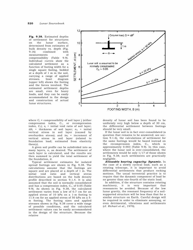
520 Lunar Sourcebook
where Cj = compressibility of soil layer j (either compression index, Cc, or recompression index, Cr); ej = initial void ratio of soil layer; ∆Hj = thickness of soil layer; σij = initial vertical stress in soil layer (caused by overburden stress); and ∆σj = increment of vertical stress in soil layer (related to foundation load; estimated from elasticity theory).
A given soil profile can be subdivided into as many layers, n, as desired. The settlement of each layer is calculated, and the results are then summed to yield the total settlement of the foundation, d.
Typical settlement estimates for isolated spread footings are shown in Fig. 9.38. The calculations assume that the footings are square and are placed at a depth of 1 m. The initial void ratio and vertical stress distributions are based on the bulk density profile described in section 9.1.4. It is also assumed that the soil is normally consolidated and has a compression index, Cc, of 0.05 (Table 9.9). As shown in Fig. 9.38, the calculated settlement varies from a low of 0.7 cm for an applied stress of 10 kPa on a 1-m footing to 11.6 cm for an applied stress of 50 kPa on a 5-m footing. The footing sizes and applied stresses shown in Fig. 9.38 cover a wide range of possible conditions, and the calculated settlement values can be easily accommodated in the design of the structure. Because the relative
density of lunar soil has been found to be uniformly very high below a depth of 30 cm, the differential settlement between footings should be very small.
If the lunar soil is in fact over-consolidated (a question that remains to be answered; see sec-tion 9.1.6), the calculations of settlement for the same footings would be based instead on the recompression index, Cr, which is approximately 0.003 (Table 9.9). In this case, where the lunar soil is over-consolidated, the settlements would be only 1/17 of those shown in Fig. 9.38; such settlements are practically negligible.
Allowable bearing capacity: Dynamic. In the case of a slowly cyclical load, such as a rotating telescope, it is important to avoid differential settlements that produce rocking motions. The usual terrestrial practice is to require that the dynamic component of load be no greater than one-fourth of the static load.
In addition, if the structure contains rotating machinery, it is very important that resonances be avoided. Because of the low lunar gravity, the resonant frequency of a soil-supported structure will be less than that for a similar structure on Earth. Careful design will be required in order to eliminate annoying, or even detrimental, vibrations and settlements (cf. Richart et al., 1970).
Fig. 9.38. Estimated depthsof settlement for structureson the lunar surface,determined from estimates ofbulk density vs. depth (Fig.9.16) combined withmeasurements ofcompressibility (Table 9.9).Individual curves show thecalculated settlement as afunction of footing width for asingle square footing, beddedat a depth of 1 m in the soil,carrying a range of appliedstresses. Inset diagram(upper left) shows the footingand the forces involved. Theestimated settlement depthsare small, even for heavyloads, and they can be easilyaccommodated in the designand construction of actuallunar structures.
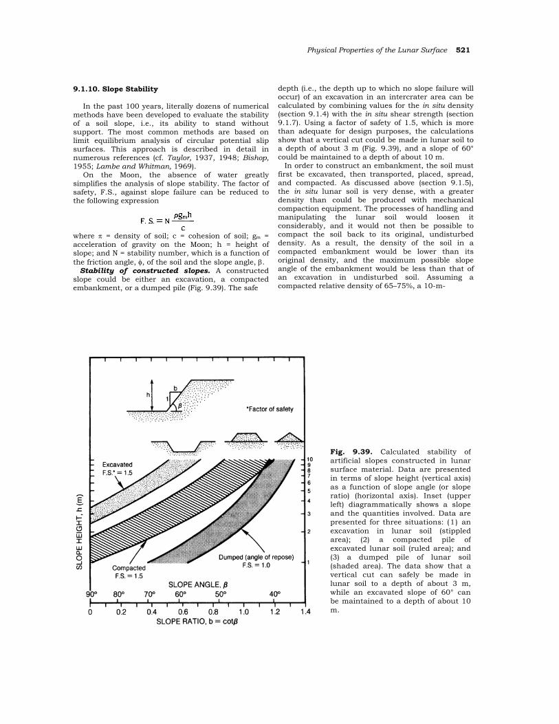
Physical Properties of the Lunar Surface 521
9.1.10. Slope Stability
In the past 100 years, literally dozens of numerical methods have been developed to evaluate the stability of a soil slope, i.e., its ability to stand without support. The most common methods are based on limit equilibrium analysis of circular potential slip surfaces. This approach is described in detail in numerous references (cf. Taylor, 1937, 1948; Bishop, 1955; Lambe and Whitman, 1969).
On the Moon, the absence of water greatly simplifies the analysis of slope stability. The factor of safety, F.S., against slope failure can be reduced to the following expression
where π = density of soil; c = cohesion of soil; gm = acceleration of gravity on the Moon; h = height of slope; and N = stability number, which is a function of the friction angle, φ, of the soil and the slope angle, β.
Stability of constructed slopes. A constructed slope could be either an excavation, a compacted embankment, or a dumped pile (Fig. 9.39). The safe
depth (i.e., the depth up to which no slope failure will occur) of an excavation in an intercrater area can be calculated by combining values for the in situ density (section 9.1.4) with the in situ shear strength (section 9.1.7). Using a factor of safety of 1.5, which is more than adequate for design purposes, the calculations show that a vertical cut could be made in lunar soil to a depth of about 3 m (Fig. 9.39), and a slope of 60° could be maintained to a depth of about 10 m.
In order to construct an embankment, the soil must first be excavated, then transported, placed, spread, and compacted. As discussed above (section 9.1.5), the in situ lunar soil is very dense, with a greater density than could be produced with mechanical compaction equipment. The processes of handling and manipulating the lunar soil would loosen it considerably, and it would not then be possible to compact the soil back to its original, undisturbed density. As a result, the density of the soil in a compacted embankment would be lower than its original density, and the maximum possible slope angle of the embankment would be less than that of an excavation in undisturbed soil. Assuming a compacted relative density of 65–75%, a 10-m-
Fig. 9.39. Calculated stability ofartificial slopes constructed in lunarsurface material. Data are presentedin terms of slope height (vertical axis)as a function of slope angle (or sloperatio) (horizontal axis). Inset (upperleft) diagrammatically shows a slopeand the quantities involved. Data arepresented for three situations: (1) anexcavation in lunar soil (stippledarea); (2) a compacted pile ofexcavated lunar soil (ruled area); and(3) a dumped pile of lunar soil(shaded area). The data show that avertical cut can safely be made inlunar soil to a depth of about 3 m,while an excavated slope of 60° canbe maintained to a depth of about 10m.
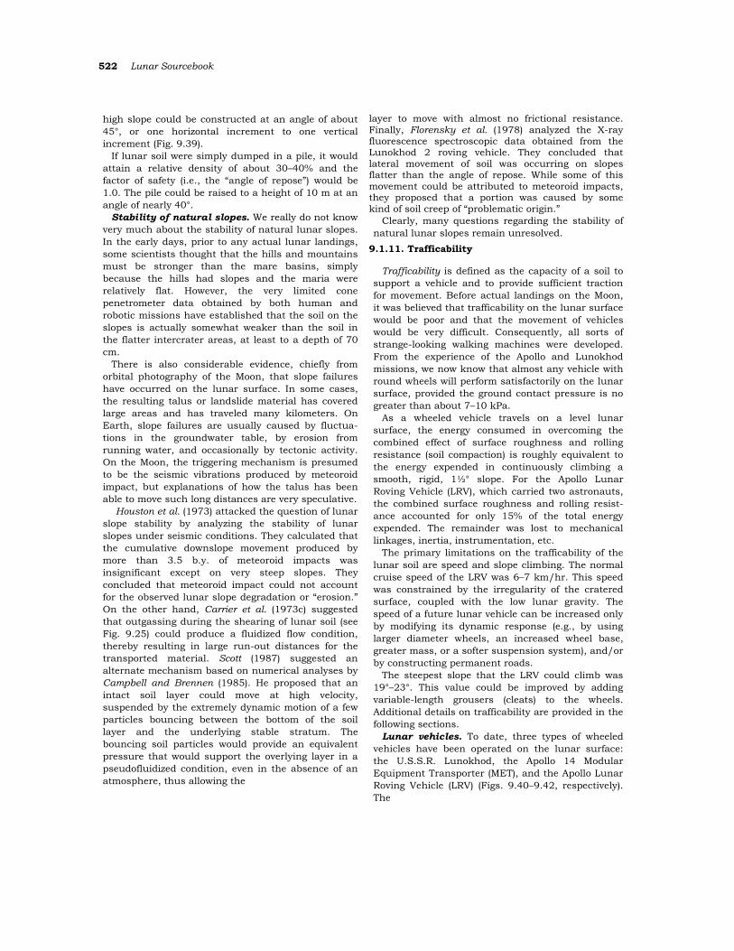
522 Lunar Sourcebook
high slope could be constructed at an angle of about 45°, or one horizontal increment to one vertical increment (Fig. 9.39).
If lunar soil were simply dumped in a pile, it would attain a relative density of about 30–40% and the factor of safety (i.e., the “angle of repose”) would be 1.0. The pile could be raised to a height of 10 m at an angle of nearly 40°.
Stability of natural slopes. We really do not know very much about the stability of natural lunar slopes. In the early days, prior to any actual lunar landings, some scientists thought that the hills and mountains must be stronger than the mare basins, simply because the hills had slopes and the maria were relatively flat. However, the very limited cone penetrometer data obtained by both human and robotic missions have established that the soil on the slopes is actually somewhat weaker than the soil in the flatter intercrater areas, at least to a depth of 70 cm.
There is also considerable evidence, chiefly from orbital photography of the Moon, that slope failures have occurred on the lunar surface. In some cases, the resulting talus or landslide material has covered large areas and has traveled many kilometers. On Earth, slope failures are usually caused by fluctua-tions in the groundwater table, by erosion from running water, and occasionally by tectonic activity. On the Moon, the triggering mechanism is presumed to be the seismic vibrations produced by meteoroid impact, but explanations of how the talus has been able to move such long distances are very speculative.
Houston et al. (1973) attacked the question of lunar slope stability by analyzing the stability of lunar slopes under seismic conditions. They calculated that the cumulative downslope movement produced by more than 3.5 b.y. of meteoroid impacts was insignificant except on very steep slopes. They concluded that meteoroid impact could not account for the observed lunar slope degradation or “erosion.” On the other hand, Carrier et al. (1973c) suggested that outgassing during the shearing of lunar soil (see Fig. 9.25) could produce a fluidized flow condition, thereby resulting in large run-out distances for the transported material. Scott (1987) suggested an alternate mechanism based on numerical analyses by Campbell and Brennen (1985). He proposed that an intact soil layer could move at high velocity, suspended by the extremely dynamic motion of a few particles bouncing between the bottom of the soil layer and the underlying stable stratum. The bouncing soil particles would provide an equivalent pressure that would support the overlying layer in a pseudofluidized condition, even in the absence of an atmosphere, thus allowing the
layer to move with almost no frictional resistance. Finally, Florensky et al. (1978) analyzed the X-ray fluorescence spectroscopic data obtained from the Lunokhod 2 roving vehicle. They concluded that lateral movement of soil was occurring on slopes flatter than the angle of repose. While some of this movement could be attributed to meteoroid impacts, they proposed that a portion was caused by some kind of soil creep of “problematic origin.”
Clearly, many questions regarding the stability of natural lunar slopes remain unresolved.
9.1.11. Trafficability
Trafficability is defined as the capacity of a soil to support a vehicle and to provide sufficient traction for movement. Before actual landings on the Moon, it was believed that trafficability on the lunar surface would be poor and that the movement of vehicles would be very difficult. Consequently, all sorts of strange-looking walking machines were developed. From the experience of the Apollo and Lunokhod missions, we now know that almost any vehicle with round wheels will perform satisfactorily on the lunar surface, provided the ground contact pressure is no greater than about 7–10 kPa.
As a wheeled vehicle travels on a level lunar surface, the energy consumed in overcoming the combined effect of surface roughness and rolling resistance (soil compaction) is roughly equivalent to the energy expended in continuously climbing a smooth, rigid, 1½° slope. For the Apollo Lunar Roving Vehicle (LRV), which carried two astronauts, the combined surface roughness and rolling resist-ance accounted for only 15% of the total energy expended. The remainder was lost to mechanical linkages, inertia, instrumentation, etc.
The primary limitations on the trafficability of the lunar soil are speed and slope climbing. The normal cruise speed of the LRV was 6–7 km/hr. This speed was constrained by the irregularity of the cratered surface, coupled with the low lunar gravity. The speed of a future lunar vehicle can be increased only by modifying its dynamic response (e.g., by using larger diameter wheels, an increased wheel base, greater mass, or a softer suspension system), and/or by constructing permanent roads.
The steepest slope that the LRV could climb was 19°–23°. This value could be improved by adding variable-length grousers (cleats) to the wheels. Additional details on trafficability are provided in the following sections.
Lunar vehicles. To date, three types of wheeled vehicles have been operated on the lunar surface: the U.S.S.R. Lunokhod, the Apollo 14 Modular Equipment Transporter (MET), and the Apollo Lunar Roving Vehicle (LRV) (Figs. 9.40–9.42, respectively). The
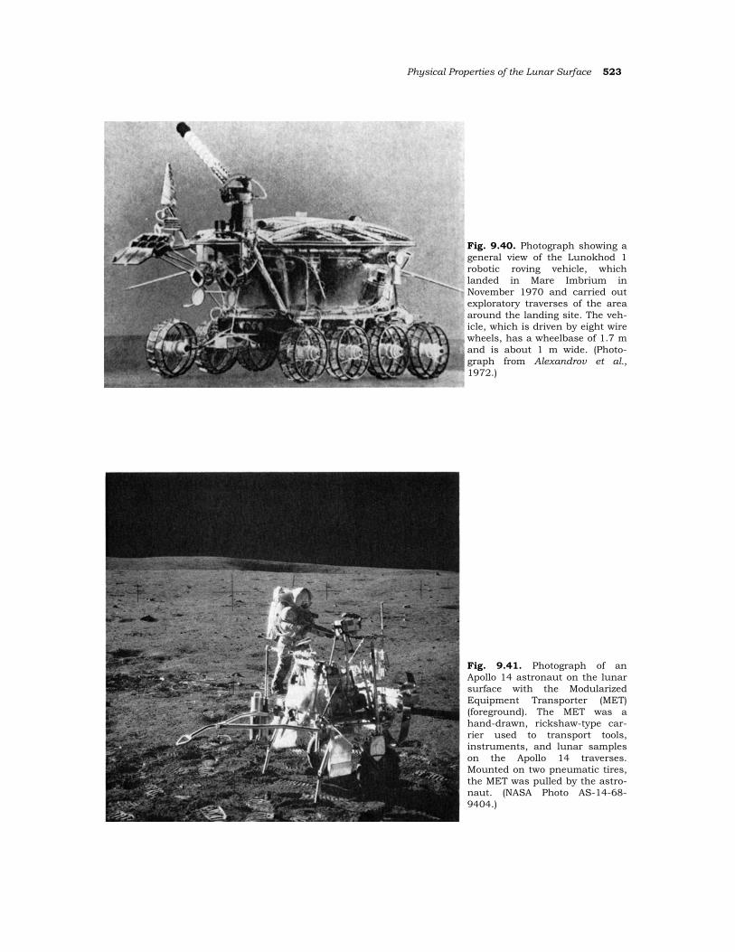
Physical Properties of the Lunar Surface 523
Fig. 9.40. Photograph showing a general view of the Lunokhod 1 robotic roving vehicle, which landed in Mare Imbrium in November 1970 and carried out exploratory traverses of the area around the landing site. The veh-icle, which is driven by eight wire wheels, has a wheelbase of 1.7 m and is about 1 m wide. (Photo-graph from Alexandrov et al., 1972.)
Fig. 9.41. Photograph of an Apollo 14 astronaut on the lunar surface with the Modularized Equipment Transporter (MET) (foreground). The MET was a hand-drawn, rickshaw-type car-rier used to transport tools, instruments, and lunar samples on the Apollo 14 traverses. Mounted on two pneumatic tires, the MET was pulled by the astro-naut. (NASA Photo AS-14-68-9404.)
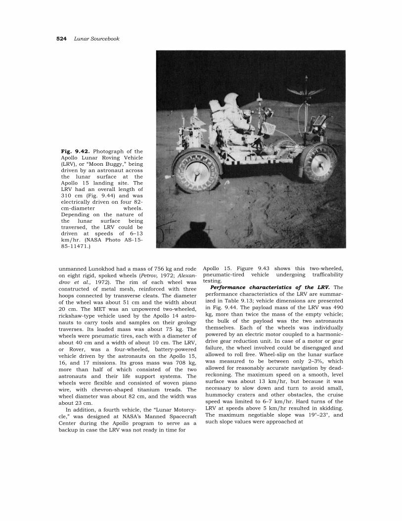
524 Lunar Sourcebook
unmanned Lunokhod had a mass of 756 kg and rode on eight rigid, spoked wheels (Petrov, 1972; Alexan-drov et al., 1972). The rim of each wheel was constructed of metal mesh, reinforced with three hoops connected by transverse cleats. The diameter of the wheel was about 51 cm and the width about 20 cm. The MET was an unpowered two-wheeled, rickshaw-type vehicle used by the Apollo 14 astro-nauts to carry tools and samples on their geology traverses. Its loaded mass was about 75 kg. The wheels were pneumatic tires, each with a diameter of about 40 cm and a width of about 10 cm. The LRV, or Rover, was a four-wheeled, battery-powered vehicle driven by the astronauts on the Apollo 15, 16, and 17 missions. Its gross mass was 708 kg, more than half of which consisted of the two astronauts and their life support systems. The wheels were flexible and consisted of woven piano wire, with chevron-shaped titanium treads. The wheel diameter was about 82 cm, and the width was about 23 cm.
In addition, a fourth vehicle, the “Lunar Motorcy-cle,” was designed at NASA’s Manned Spacecraft Center during the Apollo program to serve as a backup in case the LRV was not ready in time for
Apollo 15. Figure 9.43 shows this two-wheeled, pneumatic-tired vehicle undergoing trafficability testing.
Performance characteristics of the LRV. The performance characteristics of the LRV are summar-ized in Table 9.13; vehicle dimensions are presented in Fig. 9.44. The payload mass of the LRV was 490 kg, more than twice the mass of the empty vehicle; the bulk of the payload was the two astronauts themselves. Each of the wheels was individually powered by an electric motor coupled to a harmonic-drive gear reduction unit. In case of a motor or gear failure, the wheel involved could be disengaged and allowed to roll free. Wheel-slip on the lunar surface was measured to be between only 2–3%, which allowed for reasonably accurate navigation by dead-reckoning. The maximum speed on a smooth, level surface was about 13 km/hr, but because it was necessary to slow down and turn to avoid small, hummocky craters and other obstacles, the cruise speed was limited to 6–7 km/hr. Hard turns of the LRV at speeds above 5 km/hr resulted in skidding. The maximum negotiable slope was 19°–23°, and such slope values were approached at
Fig. 9.42. Photograph of theApollo Lunar Roving Vehicle(LRV), or “Moon Buggy,” beingdriven by an astronaut acrossthe lunar surface at theApollo 15 landing site. TheLRV had an overall length of310 cm (Fig. 9.44) and waselectrically driven on four 82-cm-diameter wheels.Depending on the nature ofthe lunar surface beingtraversed, the LRV could bedriven at speeds of 6–13km/hr. (NASA Photo AS-15-85-11471.)
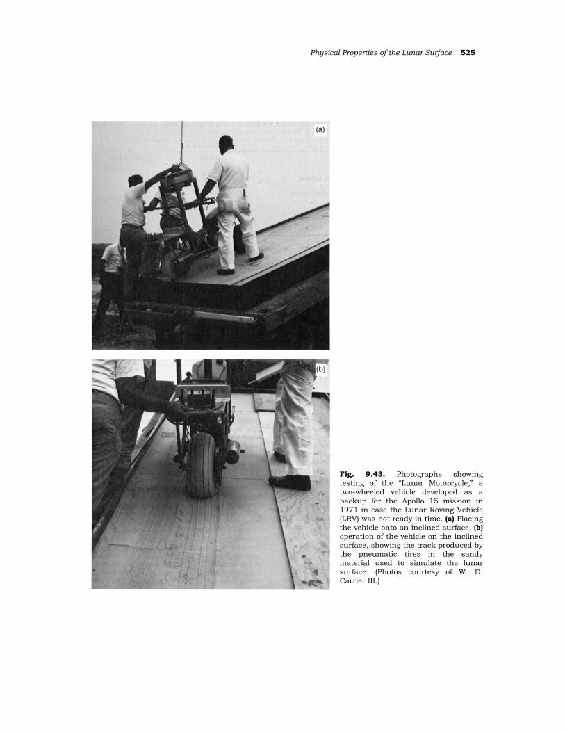
Physical Properties of the Lunar Surface 525
Fig. 9.43. Photographs showing testing of the “Lunar Motorcycle,” a two-wheeled vehicle developed as a backup for the Apollo 15 mission in 1971 in case the Lunar Roving Vehicle (LRV) was not ready in time. (a) Placing the vehicle onto an inclined surface; (b) operation of the vehicle on the inclined surface, showing the track produced by the pneumatic tires in the sandy material used to simulate the lunar surface. (Photos courtesy of W. D. Carrier III.)
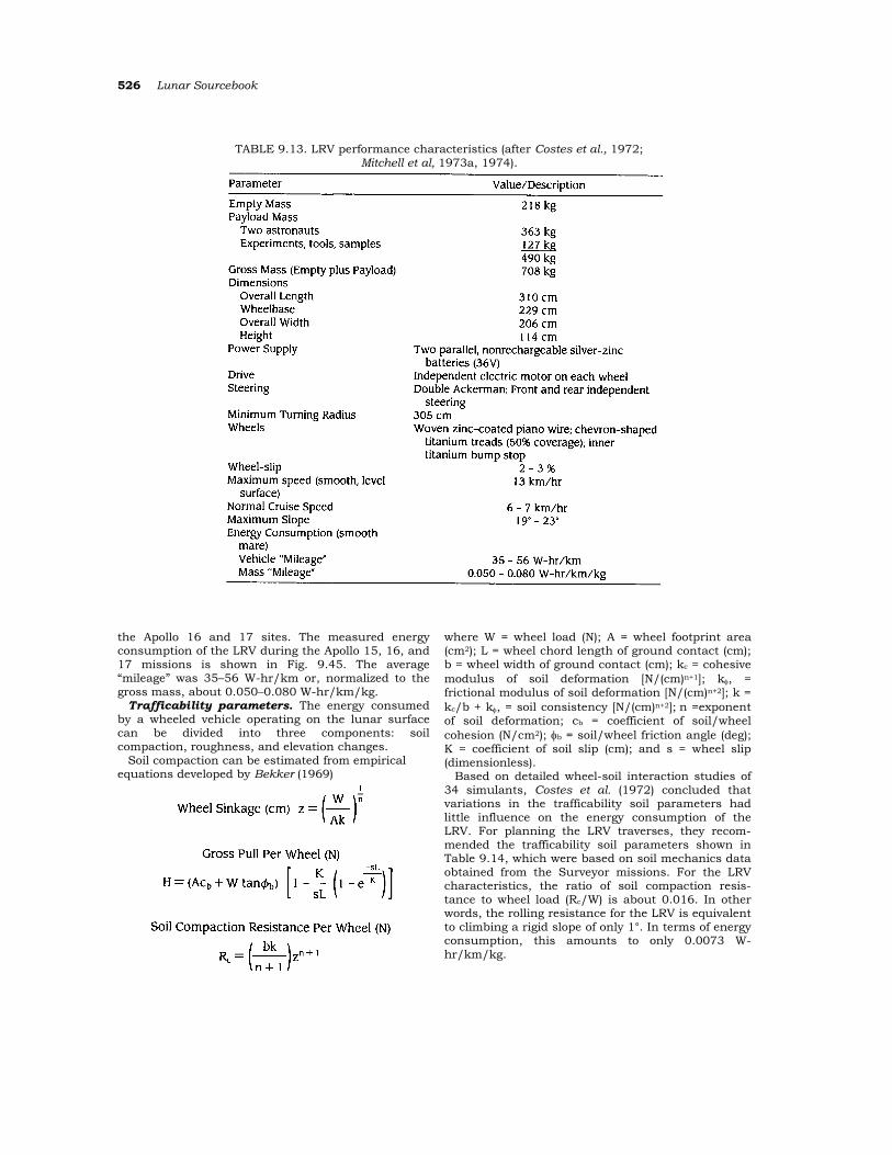
526 Lunar Sourcebook
TABLE 9.13. LRV performance characteristics (after Costes et al., 1972; Mitchell et al, 1973a, 1974).
the Apollo 16 and 17 sites. The measured energy consumption of the LRV during the Apollo 15, 16, and 17 missions is shown in Fig. 9.45. The average “mileage” was 35–56 W-hr/km or, normalized to the gross mass, about 0.050–0.080 W-hr/km/kg.
Trafficability parameters. The energy consumed by a wheeled vehicle operating on the lunar surface can be divided into three components: soil compaction, roughness, and elevation changes.
Soil compaction can be estimated from empirical equations developed by Bekker (1969)
where W = wheel load (N); A = wheel footprint area (cm2); L = wheel chord length of ground contact (cm); b = wheel width of ground contact (cm); kc = cohesive modulus of soil deformation [N/(cm)n+1]; kφ, = frictional modulus of soil deformation [N/(cm)n+2]; k = kc/b + kφ, = soil consistency [N/(cm)n+2]; n =exponent of soil deformation; cb = coefficient of soil/wheel cohesion (N/cm2); φb = soil/wheel friction angle (deg); K = coefficient of soil slip (cm); and s = wheel slip (dimensionless).
Based on detailed wheel-soil interaction studies of 34 simulants, Costes et al. (1972) concluded that variations in the trafficability soil parameters had little influence on the energy consumption of the LRV. For planning the LRV traverses, they recom-mended the trafficability soil parameters shown in Table 9.14, which were based on soil mechanics data obtained from the Surveyor missions. For the LRV characteristics, the ratio of soil compaction resis-tance to wheel load (Rc/W) is about 0.016. In other words, the rolling resistance for the LRV is equivalent to climbing a rigid slope of only 1°. In terms of energy consumption, this amounts to only 0.0073 W-hr/km/kg.
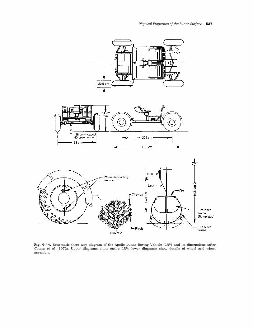
Physical Properties of the Lunar Surface 527
Fig. 9.44. Schematic three-way diagram of the Apollo Lunar Roving Vehicle (LRV) and its dimensions (after Costes et al., 1972). Upper diagrams show entire LRV; lower diagrams show details of wheel and wheel assembly.
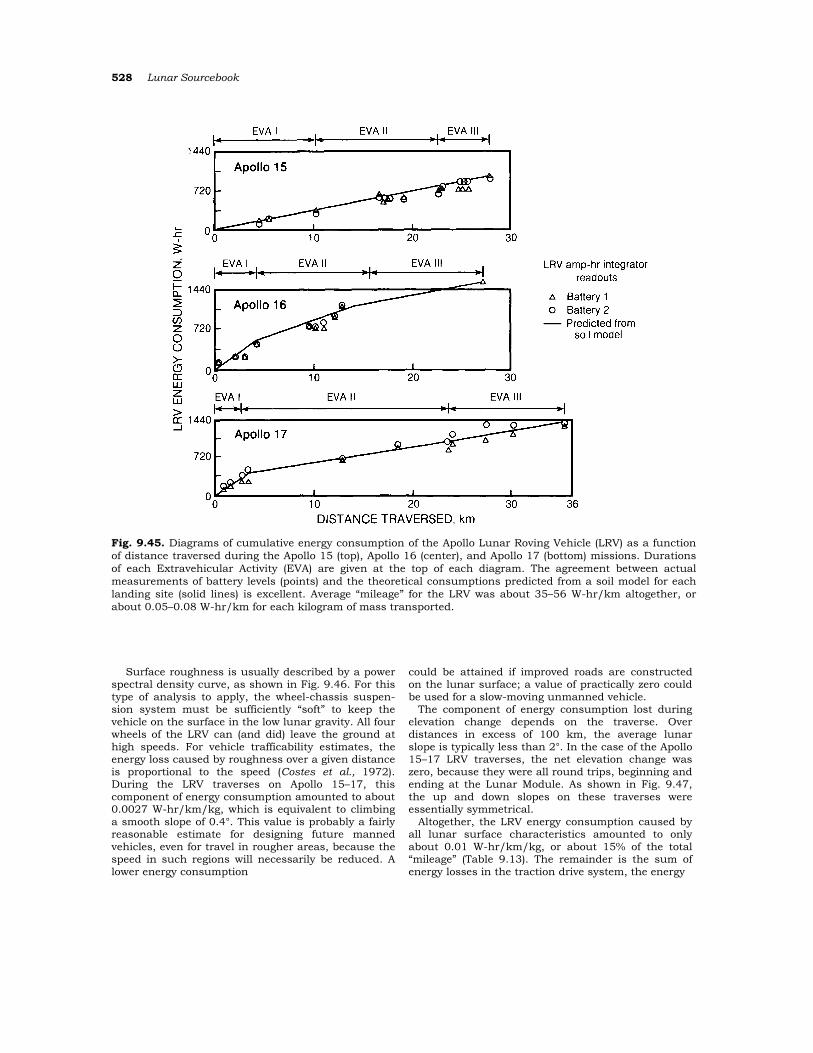
528 Lunar Sourcebook
Fig. 9.45. Diagrams of cumulative energy consumption of the Apollo Lunar Roving Vehicle (LRV) as a function of distance traversed during the Apollo 15 (top), Apollo 16 (center), and Apollo 17 (bottom) missions. Durations of each Extravehicular Activity (EVA) are given at the top of each diagram. The agreement between actual measurements of battery levels (points) and the theoretical consumptions predicted from a soil model for each landing site (solid lines) is excellent. Average “mileage” for the LRV was about 35–56 W-hr/km altogether, or about 0.05–0.08 W-hr/km for each kilogram of mass transported.
Surface roughness is usually described by a power spectral density curve, as shown in Fig. 9.46. For this type of analysis to apply, the wheel-chassis suspen-sion system must be sufficiently “soft” to keep the vehicle on the surface in the low lunar gravity. All four wheels of the LRV can (and did) leave the ground at high speeds. For vehicle trafficability estimates, the energy loss caused by roughness over a given distance is proportional to the speed (Costes et al., 1972). During the LRV traverses on Apollo 15–17, this component of energy consumption amounted to about 0.0027 W-hr/km/kg, which is equivalent to climbing a smooth slope of 0.4°. This value is probably a fairly reasonable estimate for designing future manned vehicles, even for travel in rougher areas, because the speed in such regions will necessarily be reduced. A lower energy consumption
could be attained if improved roads are constructed on the lunar surface; a value of practically zero could be used for a slow-moving unmanned vehicle.
The component of energy consumption lost during elevation change depends on the traverse. Over distances in excess of 100 km, the average lunar slope is typically less than 2°. In the case of the Apollo 15–17 LRV traverses, the net elevation change was zero, because they were all round trips, beginning and ending at the Lunar Module. As shown in Fig. 9.47, the up and down slopes on these traverses were essentially symmetrical.
Altogether, the LRV energy consumption caused by all lunar surface characteristics amounted to only about 0.01 W-hr/km/kg, or about 15% of the total “mileage” (Table 9.13). The remainder is the sum of energy losses in the traction drive system, the energy
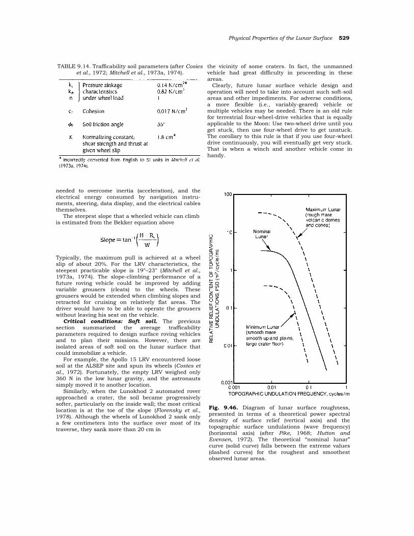
Physical Properties of the Lunar Surface 529
TABLE 9.14. Trafficability soil parameters (after Cosies et al., 1972; Mitchell et al., 1973a, 1974).
the vicinity of some craters. In fact, the unmanned vehicle had great difficulty in proceeding in these areas.
Clearly, future lunar surface vehicle design and operation will need to take into account such soft-soil areas and other impediments. For adverse conditions, a more flexible (i.e., variably-geared) vehicle or multiple vehicles may be needed. There is an old rule for terrestrial four-wheel-drive vehicles that is equally applicable to the Moon: Use two-wheel drive until you get stuck, then use four-wheel drive to get unstuck. The corollary to this rule is that if you use four-wheel drive continuously, you will eventually get very stuck. That is when a winch and another vehicle come in handy.
needed to overcome inertia (acceleration), and the electrical energy consumed by navigation instru-ments, steering, data display, and the electrical cables themselves.
The steepest slope that a wheeled vehicle can climb is estimated from the Bekker equation above
Typically, the maximum pull is achieved at a wheel slip of about 20%. For the LRV characteristics, the steepest practicable slope is 19°–23° (Mitchell et al., 1973a, 1974). The slope-climbing performance of a future roving vehicle could be improved by adding variable grousers (cleats) to the wheels. These grousers would be extended when climbing slopes and retracted for cruising on relatively flat areas. The driver would have to be able to operate the grousers without leaving his seat on the vehicle.
Critical conditions: Soft soil. The previous section summarized the average trafficability parameters required to design surface roving vehicles and to plan their missions. However, there are isolated areas of soft soil on the lunar surface that could immobilize a vehicle.
For example, the Apollo 15 LRV encountered loose soil at the ALSEP site and spun its wheels (Costes et al., 1972). Fortunately, the empty LRV weighed only 360 N in the low lunar gravity, and the astronauts simply moved it to another location.
Similarly, when the Lunokhod 2 automated rover approached a crater, the soil became progressively softer, particularly on the inside wall; the most critical location is at the toe of the slope (Florensky et al., 1978). Although the wheels of Lunokhod 2 sank only a few centimeters into the surface over most of its traverse, they sank more than 20 cm in
Fig. 9.46. Diagram of lunar surface roughness, presented in terms of a theoretical power spectral density of surface relief (vertical axis) and the topographic surface undulations (wave frequency) (horizontal axis) (after Pike, 1968; Hutton and Evensen, 1972). The theoretical “nominal lunar” curve (solid curve) falls between the extreme values (dashed curves) for the roughest and smoothest observed lunar areas.
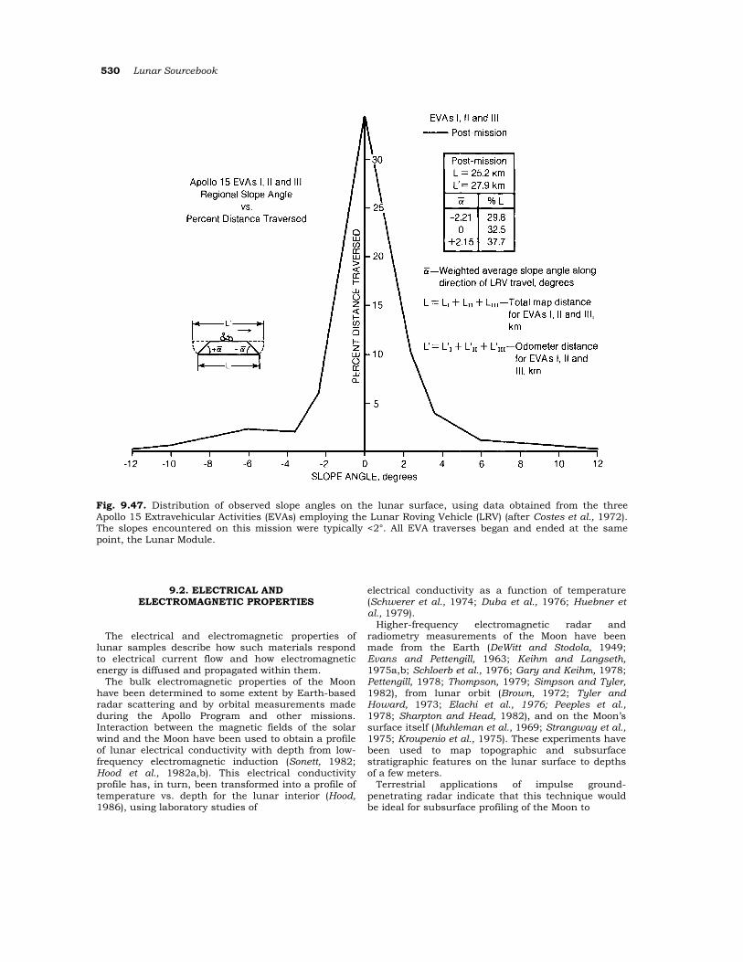
530 Lunar Sourcebook
Fig. 9.47. Distribution of observed slope angles on the lunar surface, using data obtained from the three Apollo 15 Extravehicular Activities (EVAs) employing the Lunar Roving Vehicle (LRV) (after Costes et al., 1972). The slopes encountered on this mission were typically <2°. All EVA traverses began and ended at the same point, the Lunar Module.
9.2. ELECTRICAL AND ELECTROMAGNETIC PROPERTIES
The electrical and electromagnetic properties of lunar samples describe how such materials respond to electrical current flow and how electromagnetic energy is diffused and propagated within them.
The bulk electromagnetic properties of the Moon have been determined to some extent by Earth-based radar scattering and by orbital measurements made during the Apollo Program and other missions. Interaction between the magnetic fields of the solar wind and the Moon have been used to obtain a profile of lunar electrical conductivity with depth from low-frequency electromagnetic induction (Sonett, 1982; Hood et al., 1982a,b). This electrical conductivity profile has, in turn, been transformed into a profile of temperature vs. depth for the lunar interior (Hood, 1986), using laboratory studies of
electrical conductivity as a function of temperature (Schwerer et al., 1974; Duba et al., 1976; Huebner et al., 1979).
Higher-frequency electromagnetic radar and radiometry measurements of the Moon have been made from the Earth (DeWitt and Stodola, 1949; Evans and Pettengill, 1963; Keihm and Langseth, 1975a,b; Schloerb et al., 1976; Gary and Keihm, 1978; Pettengill, 1978; Thompson, 1979; Simpson and Tyler, 1982), from lunar orbit (Brown, 1972; Tyler and Howard, 1973; Elachi et al., 1976; Peeples et al., 1978; Sharpton and Head, 1982), and on the Moon’s surface itself (Muhleman et al., 1969; Strangway et al., 1975; Kroupenio et al., 1975). These experiments have been used to map topographic and subsurface stratigraphic features on the lunar surface to depths of a few meters.
Terrestrial applications of impulse ground-penetrating radar indicate that this technique would be ideal for subsurface profiling of the Moon to
Physical Properties of the Lunar Surface 531
depths of more than 100 m (Olhoeft, 1979, 1984; Wright et al., 1984; Schaber et al.., 1986). The depth of investigation would not be limited by material intrinsic loss properties, but by the electromagnetic scattering, which would depend on the scale of heterogeneities in the subsurface.
The electrical properties of the Moon’s surface materials are those of silicates characterized by extremely low loss and low electrical conductivity. In the total absence of water, the DC electrical conductivity ranges from 10–14 mho/m for lunar soiils to 10–9 mho/m for lunar rocks at 300 K in darkness. Upon irradiation with sunlight, there is a >106 increase in electrical conductivity in both lunar soils and rocks. The relative dielectric permittivity for lunar materials is approximately
where ρ = bulk density in g/cm3. The relative dielectric permittivity is dominantly controlled by bulk density and is independent of chemical or mineralogical composition, frequency variations above 1 MHz, and temperature variations within the range of lunar surface temperatures.
The high frequency electromagnetic loss is given by
where ρ = density and tan δ = loss tangent (ratio of the imaginary to the real part of the complex dielectric permittivity). The loss is strongly dependent upon density and the (TiO2 + FeO) content, and less dependent on frequency and temperature. Electro-magnetic losses in the lunar soils have nearly negligible frequency and temperature dependence in comparison to the behavior of lunar rocks.
The extremely low electrical conductivities and low loss tangents indicate that lunar materials are very transparent to electromagnetic energy. For example, radio transmissions should readily penetrate through the lunar soils to depths of about 10 m. As a result, radio communications on the lunar surface need not be by direct line-of-sight, but may penetrate low hills; this situation partially compensates on the Moon for the inability to skip signals off an ionosphere for long distances as is done on Earth. The low conductivity and low loss are also responsible for the fact that lunar materials are readily chargeable and will remain electrically charged for long periods of time. The large photo-induced change in electrical conductivity at lunar sunrise and sunset can charge surface soil particles to the point that they will levitate and move (Alvarez, 1977a; De and Criswell, 1977; Criswell and De, 1977;
Rhee et al., 1977; McDonnell, 1979; Ip, 1986). Such charged soils and mobile particles could readily coat surfaces and be hazardous to visibility and equipment operation during lunar night.
9.2.1. Electrical Conductivity
Electrical conductivity is a measure of how easily electrical current flows through a material, i.e., how easily electrical charge may be transported through it. High electrical conductivity means that the material easily carries electrical current and does not readily remain electrically charged. Low electrical conductivity means that the material does not easily transport charge and tends to remain electrically charged. The electrical conductivity of lunar materials at low frequencies (below 1 Hz) is essentially the same as of DC (0 Hz) conductivity, is extremely low (Table 9.15), and is dominantly controlled by temperature. A soil from the Apollo 15 site (sample 15301,38) exhibits a temperature dependence of conductivity (Fig. 9.48) of the form
where T = temperature (Kelvin) (Olhoeft et al., 1974a). This type of temperature dependence is characteristic of amorphous materials and is typical of the heavily radiation-damaged lunar soil particles. The low-frequency electrical conductivity of lunar rocks is typical of terrestrial silicates in the total absence of water. The temperature dependence of one Apollo 16 rock (sample 65015,6) (Olhoeft et al., 1973a) was similar in form to that of soil
However, the temperature dependence of the electrical conductivity measured on the remaining lunar rocks (Fig. 9.48) was found to be given by
where k = Boltzmann’s constant = 8.6176 × 10⁻⁵ eV/K and T = temperature (Kelvin), and E0 and E1 are activation energies (Table 9.15). Because these lunar materials have very low conductivities, dielectric relaxation effects and displacement currents dominate at very low frequencies. Olhoeft et al. (1973a) and Schwerer et al. (1974) provide the best reviews of electrical conductivity of lunar rocks.
The electrical conductivities measured on lunar samples (Schwerer et al., 1972, 1973, 1974; Olhoeft et al., 1973a,b, 1974b) and related materials (Housley and Morin, 1972; Piwinskii and Duba, 1975; Duba et al., 1976, 1979; Huebner et al., 1978, 1979; Schock et al., 1980) are key parameters in using the data
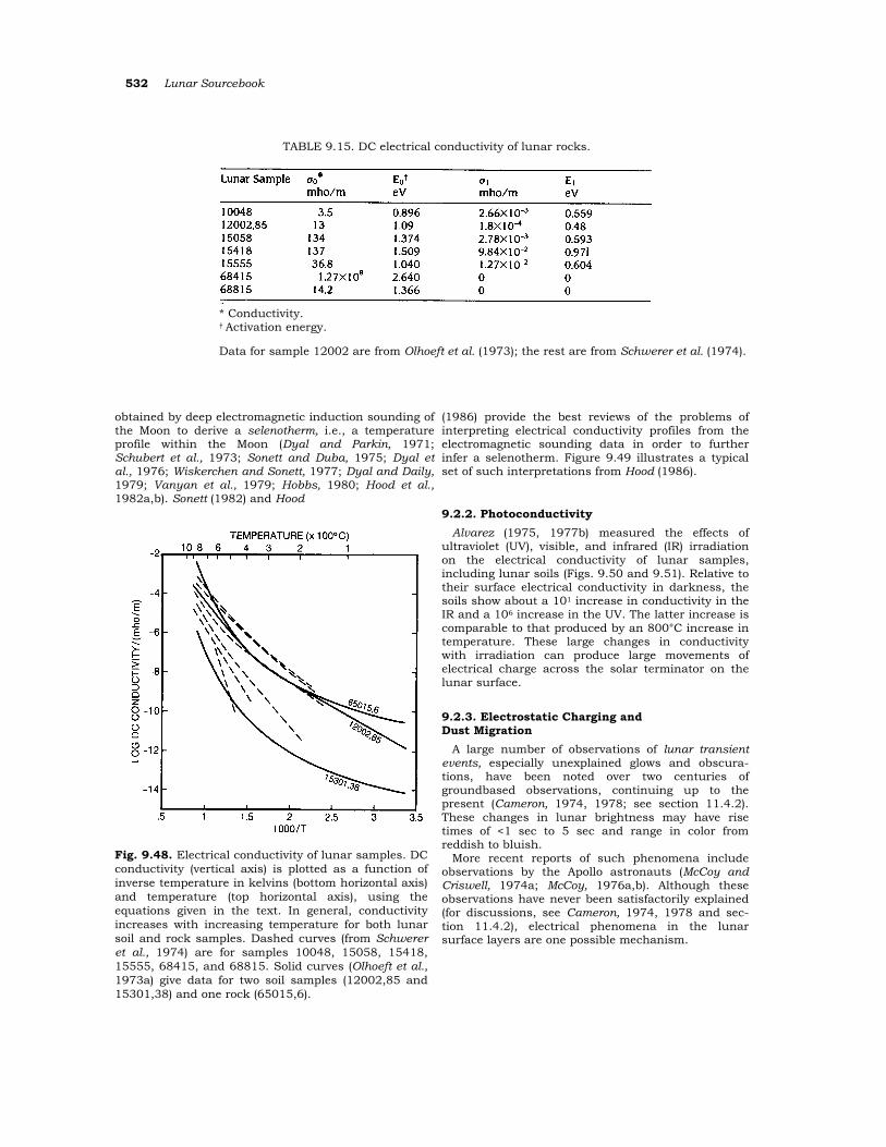
532 Lunar Sourcebook
TABLE 9.15. DC electrical conductivity of lunar rocks.
* Conductivity. † Activation energy.
Data for sample 12002 are from Olhoeft et al. (1973); the rest are from Schwerer et al. (1974).
obtained by deep electromagnetic induction sounding of the Moon to derive a selenotherm, i.e., a temperature profile within the Moon (Dyal and Parkin, 1971; Schubert et al., 1973; Sonett and Duba, 1975; Dyal et al., 1976; Wiskerchen and Sonett, 1977; Dyal and Daily, 1979; Vanyan et al., 1979; Hobbs, 1980; Hood et al., 1982a,b). Sonett (1982) and Hood
Fig. 9.48. Electrical conductivity of lunar samples. DC conductivity (vertical axis) is plotted as a function of inverse temperature in kelvins (bottom horizontal axis) and temperature (top horizontal axis), using the equations given in the text. In general, conductivity increases with increasing temperature for both lunar soil and rock samples. Dashed curves (from Schwerer et al., 1974) are for samples 10048, 15058, 15418, 15555, 68415, and 68815. Solid curves (Olhoeft et al., 1973a) give data for two soil samples (12002,85 and 15301,38) and one rock (65015,6).
(1986) provide the best reviews of the problems of interpreting electrical conductivity profiles from the electromagnetic sounding data in order to further infer a selenotherm. Figure 9.49 illustrates a typical set of such interpretations from Hood (1986).
9.2.2. Photoconductivity Alvarez (1975, 1977b) measured the effects of
ultraviolet (UV), visible, and infrared (IR) irradiation on the electrical conductivity of lunar samples, including lunar soils (Figs. 9.50 and 9.51). Relative to their surface electrical conductivity in darkness, the soils show about a 101 increase in conductivity in the IR and a 106 increase in the UV. The latter increase is comparable to that produced by an 800°C increase in temperature. These large changes in conductivity with irradiation can produce large movements of electrical charge across the solar terminator on the lunar surface.
9.2.3. Electrostatic Charging and Dust Migration
A large number of observations of lunar transient events, especially unexplained glows and obscura-tions, have been noted over two centuries of groundbased observations, continuing up to the present (Cameron, 1974, 1978; see section 11.4.2). These changes in lunar brightness may have rise times of <1 sec to 5 sec and range in color from reddish to bluish.
More recent reports of such phenomena include observations by the Apollo astronauts (McCoy and Criswell, 1974a; McCoy, 1976a,b). Although these observations have never been satisfactorily explained (for discussions, see Cameron, 1974, 1978 and sec-tion 11.4.2), electrical phenomena in the lunar surface layers are one possible mechanism.
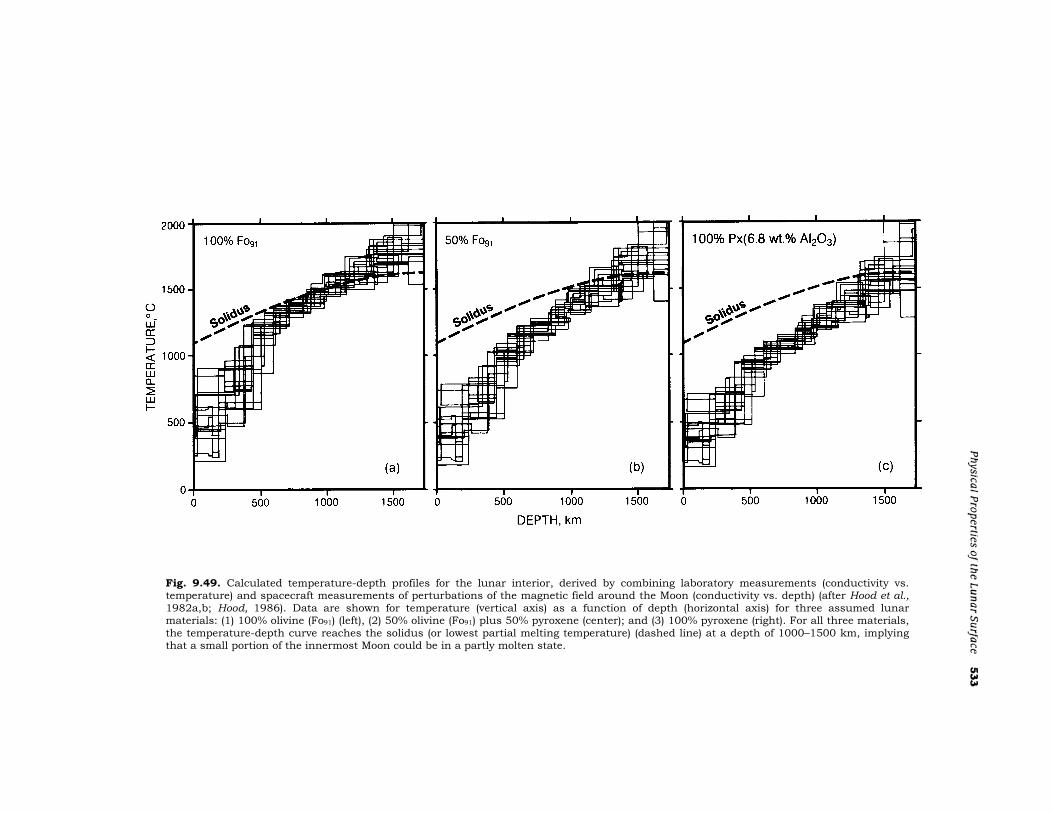
Fig. 9.49. Calculated temperature-depth profiles for the lunar interior, derived by combining laboratory measurements (conductivity vs. temperature) and spacecraft measurements of perturbations of the magnetic field around the Moon (conductivity vs. depth) (after Hood et al., 1982a,b; Hood, 1986). Data are shown for temperature (vertical axis) as a function of depth (horizontal axis) for three assumed lunar materials: (1) 100% olivine (Fo91) (left), (2) 50% olivine (Fo91) plus 50% pyroxene (center); and (3) 100% pyroxene (right). For all three materials, the temperature-depth curve reaches the solidus (or lowest partial melting temperature) (dashed line) at a depth of 1000–1500 km, implying that a small portion of the innermost Moon could be in a partly molten state.
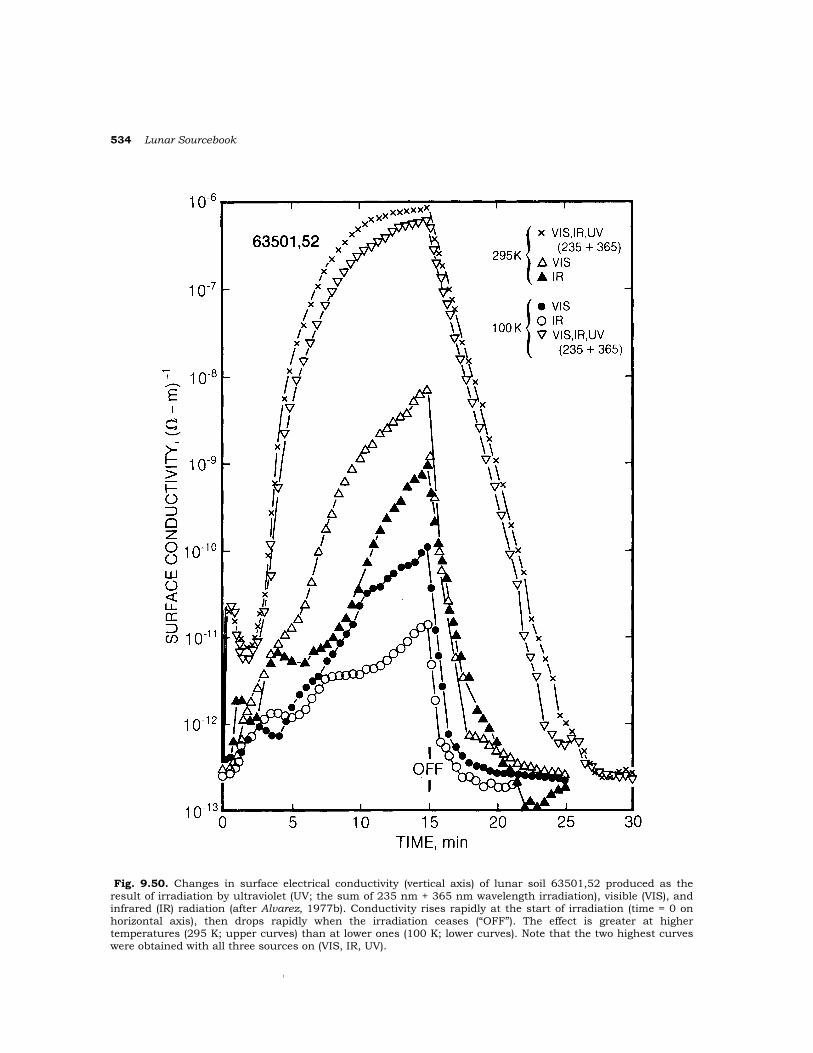
534 Lunar Sourcebook
Fig. 9.50. Changes ίn surface electrical conductivity (vertical axis) of lunar soil 63501,52 produced as the result of irradiation by ultraviolet (UV; the sum of 235 nm + 365 nm wavelength irradiation), visible (VIS), and infrared (IR) radiation (after Alvarez, 1977b). Conductivity rises rapidly at the start of irradiation (time = 0 on horizontal axis), then drops rapidly when the irradiation ceases (“OFF”). The effect is greater at higher temperatures (295 K; upper curves) than at lower ones (100 K; lower curves). Note that the two highest curves were obtained with all three sources on (VIS, IR, UV).
Ι
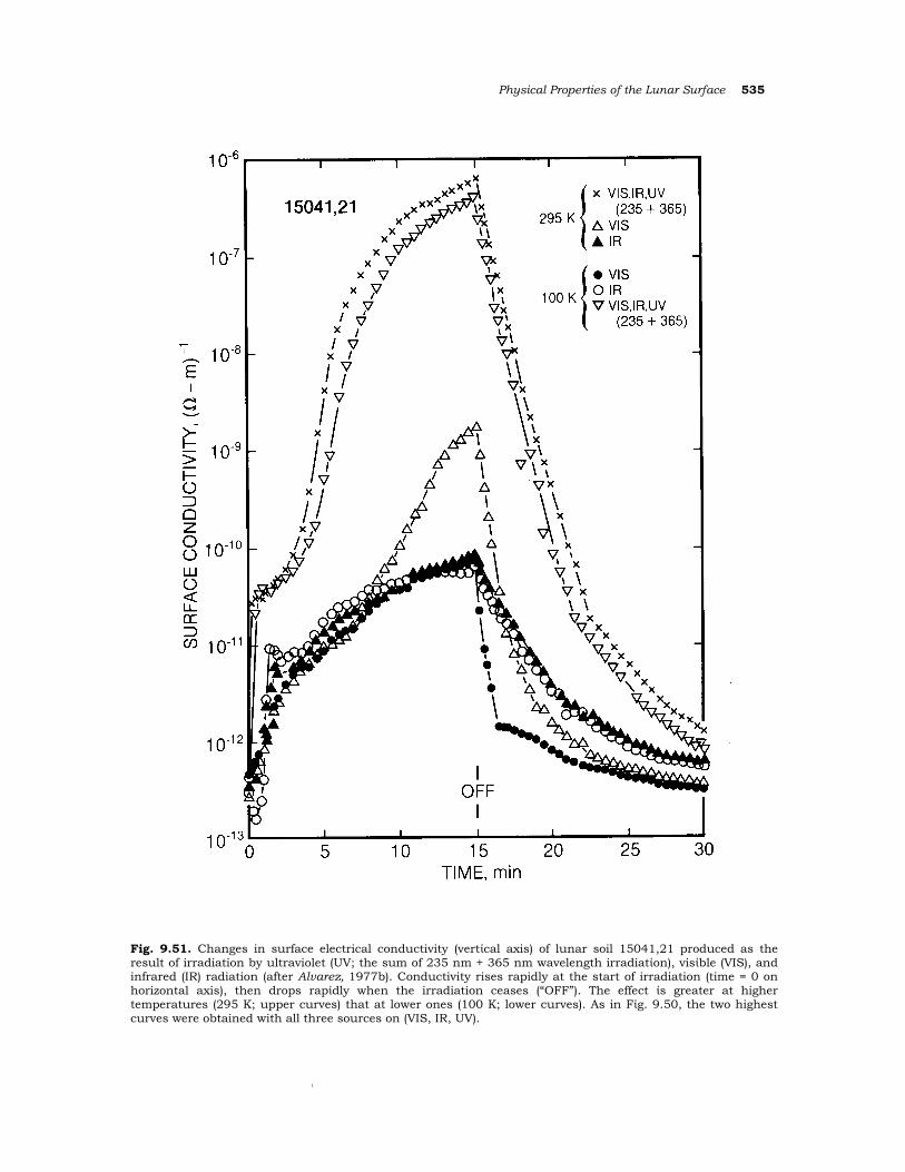
Physical Properties of the Lunar Surface 535
Fig. 9.51. Changes in surface electrical conductivity (vertίcal axis) of lunar soil 15041,21 produced as the result of irradiation by ultraviolet (UV; the sum of 235 nm + 365 nm wavelength irradiatίon), visίble (VIS), and infrared (IR) radiation (after Alvarez, 1977b). Conductivity rises rapidly at the start of irradiation (time = 0 on horizontal axis), then drops rapίdly when the irradiation ceases (“OFF”). The effect ίs greater at higher temperatures (295 K; upper curves) that at lower ones (100 K; lower curves). As in Fίg. 9.50, the two highest curves were obtained with all three sources on (VIS, IR, UV).
Ι
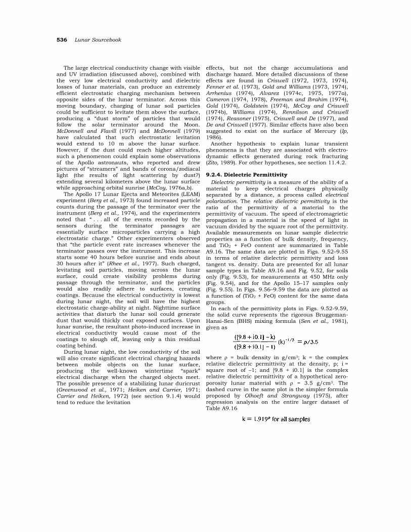
536 Lunar Sourcebook
The large electrical conductivity change with visible and UV irradiation (discussed above), combined with the very low electrical conductivίty and dίelectric losses of lunar materials, can produce an extremely efficient electrostatic charging mechanism between opposite sides of the lunar terminator. Across this moving boundary, charging of lunar soil particles could be sufficient to levitate them above the surface, producing a “dust storm” of particles that would follow the solar terminator around the Moon. McDonnell and Flavill (1977) and McDonnell (1979) have calculated that such electrostatic levitation would extend to 10 m above the lunar surface. However, if the dust could reach higher altitudes, such a phenomenon could explain some observations of the Apollo astronauts, who reported and drew pictures of “streamers” and bands of corona/zodiacal light (the results of light scattering by dust?) extending several kilometers above the lunar surface while approaching orbital sunrise (McCoy, 1976a,b).
The Apollo 17 Lunar Ejecta and Meteorites (LEAM) experiment (Berg et al., 1973) found increased particle counts during the passage of the terminator over the instrument (Berg et al., 1974), and the experimenters noted that “ . . . all of the events recorded by the sensors during the terminator passages are essentially surface microparticles carrying a high electrostatic charge.” Other experimenters observed that “the particle event rate increases whenever the terminator passes over the instrument. This increase starts some 40 hours before sunrise and ends about 30 hours after it” (Rhee et al., 1977). Such charged, levitating soil particles, moving across the lunar surface, could create visibility problems during passage through the terminator, and the particles would also readily adhere to surfaces, creating coatings. Because the electrical conductivίty is lowest during lunar night, the soil will have the highest electrostatic charge-ability at night. Nighttime surface activities that disturb the lunar soil could generate dust that would thickly coat exposed surfaces. Upon lunar sunrise, the resultant photo-induced increase in electrical conductivίty would cause most of the coatings to slough off, leaving only a thin residual coating behind.
During lunar night, the low conductivity of the soil will also create significant electrical charging hazards between mobile objects on the lunar surface, producing the well-known wintertime “spark” electrical discharge when the charged objects meet. The possible presence of a stabilizing lunar duricrust (Greenwood et al., 1971; Heiken and Carrier, 1971; Carrier and Heiken, 1972) (see section 9.1.4) would tend to reduce the levitation
effects, but not the charge accumulations and discharge hazard. More detailed discussions of these effects are found in Criswell (1972, 1973, 1974), Fenner et al. (1973), Gold and Williams (1973, 1974), Arrhenίus (1974), Alvarez (1974c, 1975, 1977α), Cameron (1974, 1978), Freeman and Ibrahim (1974), Gold (1974), Goldstein (1974), McCoy and Criswell (1974b), Williams (1974), Rennilson and Criswell (1974), Reasoner (1975), Criswell and De (1977), and De and Criswell (1977). Similar effects have also been suggested to exist on the surface of Mercury (Ip, 1986).
Another hypothesis to explain lunar transient phenomena is that they are associated with electro-dynamic effects generated during rock fracturing (Zito, 1989). For other hypotheses, see section 11.4.2.
9.2.4. Dielectric Permittivity Dielectric permittivity is a measure of the ability of a
material to keep electrical charges physically separated by a distance, a process called electrical polarization. The relative dielectric permittivity is the ratio of the permittivity of a material to the permittivity of vacuum. The speed of electromagrietic propagation in a material is the speed of light in vacuum divided by the square root of the permittivity. Available measurements on lunar sample dίelectric properties as a function of bulk density, frequency, and TiO2 + FeO content are summarized in Table Α9.16. The same data are plotted in Figs. 9.52–9.55 in terms of relative dielectric permittivity and loss tangent vs. density. Data are presented for all lunar sample types in Table Α9.16 and Fig. 9.52, for soils only (Fig. 9.53), for measurements at 450 MHz only (Fig. 9.54), and for the Apollo 15–17 samples only (Fig. 9.55). In Figs. 9.56–9.59 the data are plotted as a function of (TiO2 + FeO) content for the same data groups.
In each of the permittivity plots in Figs. 9.52-9.59, the solid curve represents the rigorous Bruggeman-Hanai-Sen (BHS) mixing formula (Sen et al., 1981), given as
where ρ = bulk density in g/cm3; k = the complex relative dielectric permittivity at the density, p; i = square root of –1; and [9.8 + i0.1] is the complex relative dίelectric permittivity of a hypothetical zero-porosity lunar material with ρ = 3.5 g/cm3. The dashed curve in the same plot is the simpler formula proposed by Olhoeft and Strangway (1975), after regression analysis on the entire larger dataset of Table Α9.16
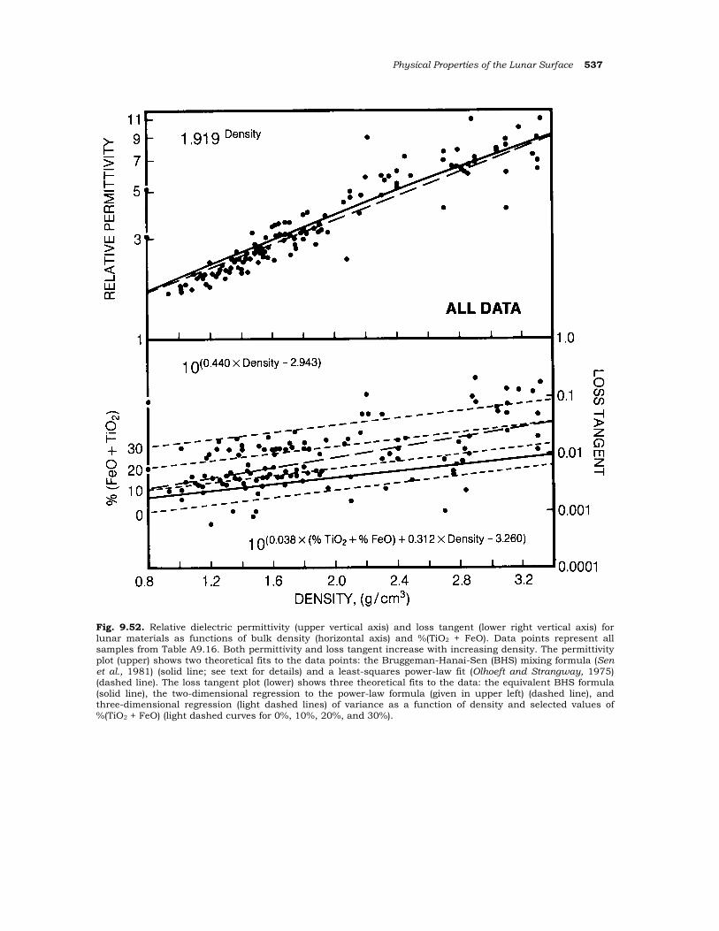
Physίcal Propertίes of the Lunar Surface 537
Fig. 9.52. Relative dielectric permittivity (upper vertical axis) and loss tangent (lower right vertical axis) for lunar materίals as functions of bulk density (horizontal axis) and %(TiO2 + FeO). Data points represent all samples from Table Α9.16. Both permittίvity and loss tangent increase with increasing density. The permittivity plot (upper) shows two theoretical fits to the data poίnts: the Bruggeman-Hanai-Sen (BHS) mixing formula (Sen et al., 1981) (solid line; see text for details) and a least-squares power-law fit (Olhoeft and Strangway, 1975) (dashed line). The loss tangent plot (lower) shows three theoretical fits to the data: the equivalent BHS formula (solid line), the two-dimensional regression to the power-law formula (given in upper left) (dashed line), and three-dimensional regressίon (light dashed lines) of variance as a function of density and selected values of %(TiO2 + FeO) (light dashed curves for 0%, 10%, 20%, and 30%).
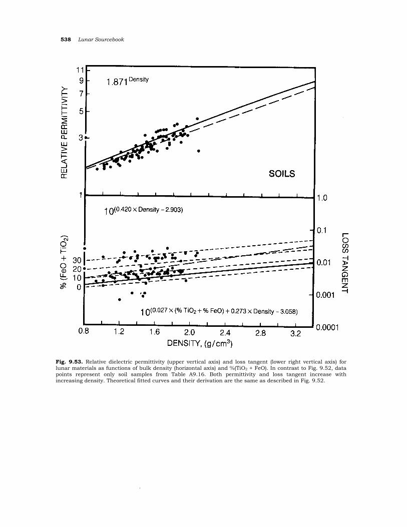
538 Lunar Sourcebook
Fig. 9.53. Relative dielectric permittivity (upper vertίcal axis) and loss tangent (lower right vertίcal axis) for lunar materίals as functions of bulk density (horizontal axίs) and %(TiO2 + FeO). In contrast to Fig. 9.52, data points represent only soil samples from Table Α9.16. Both permittivity and loss tangent increase with increasίng density. Theoretical fitted curves and their derivation are the same as described in Fig. 9.52.
Ι
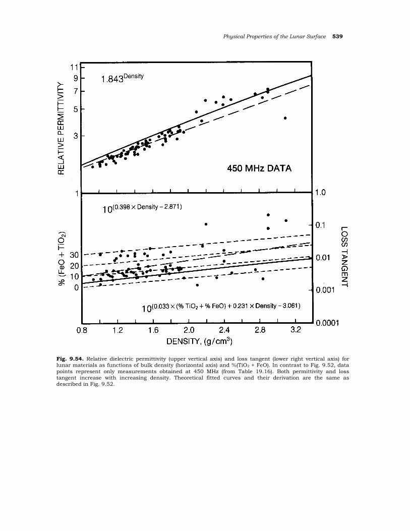
Physical Properties of the Lunar Surface 539
Fig. 9.54. Relative dielectric permittivity (upper vertical axis) and loss tangent (lower right vertical axis) for lunar materials as functίons of bulk densίty (horizontal axis) and %(TiO2 + FeO). In contrast to Fig. 9.52, data points represent only measurements obtained at 450 MHz (from Table 19.16). Both permittivity and loss tangent increase with increasing density. Theoretical fitted curves and their derivation are the same as described in Fig. 9.52.
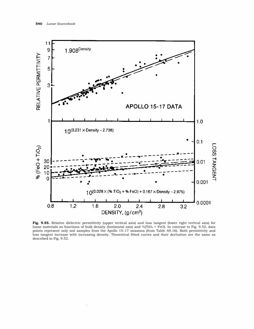
540 Lunar Sourcebook
Fig. 9.55. Relative dielectric permittivity (upper vertical axis) and loss tangent (lower right vertίcal axis) for lunar materials as functions of bulk density (horizontal axis) and %(TiO2 + FeO). In contrast to Fig. 9.52, data points represent only soil samples from the Apollo 15–17 missions (from Table A9.16). Both permittivity and loss tangent increase with increasing density. Theoretical fitted curves and their derίvatίon are the same as described in Fig. 9.52.
Ί
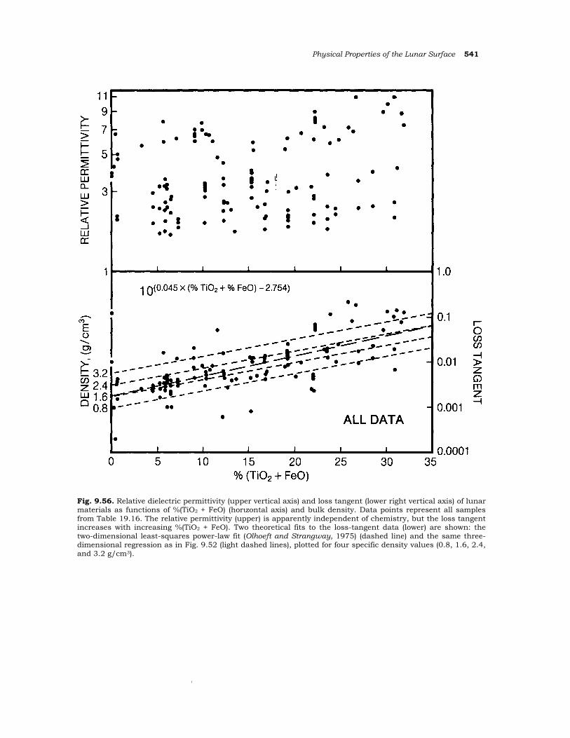
Physical Propertίes of the Lunar Surface 541
Fig. 9.56. Relative dielectric permittivity (upper vertical axis) and loss tangent (lower right vertical axis) of lunar materials as functions of %(TiO2 + FeO) (horιzontal axis) and bulk density. Data points represent all samples from Table 19.16. The relative permittivity (upper) is apparently independent of chemistry, but the loss tangent increases with increasing %(TiO2 + FeO). Two theoretical fits to the loss-tangent data (lower) are shown: the two-dimensional least-squares power-law fit (Olhoeft and Strangway, 1975) (dashed line) and the same three-dimensional regression as in Fig. 9.52 (light dashed lines), plotted for four specific density values (0.8, 1.6, 2.4, and 3.2 g/cm3).
Ι
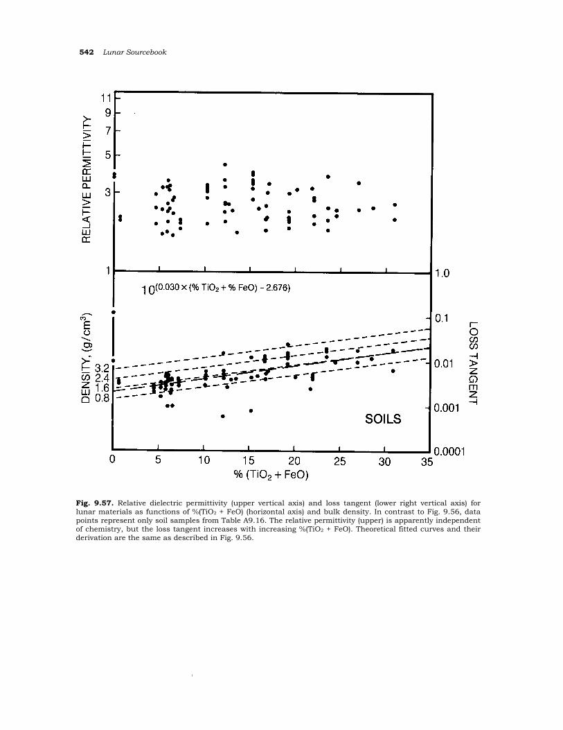
542 Lunar Sourcebook
Fig. 9.57. Relative dielectric permittivity (upper vertical axis) and loss tangent (lower right vertical axis) for lunar materials as functions of %(TiO2 + FeO) (horizontal axis) and bulk density. In contrast to Fig. 9.56, data points represent only soil samples from Table Α9.16. The relative permittivity (upper) is apparently independent of chemistry, but the loss tangent increases with increasing %(TiO2 + FeO). Theoretical fitted curves and their derivation are the same as described in Fig. 9.56.
Ι
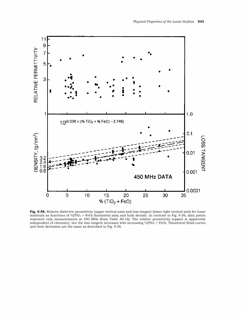
Physical Properties of the Lunar Surface 543
Fig. 9.58. Relative dielectric permittivity (upper vertical axis) and loss tangent (lower right vertical axis) for lunar materials as functίons of %(TiO2 + FeO) (horizontal axis) and bulk density. In contrast to Fig. 9.56, data points represent only measurements at 450 MHz (from Table Α9.16). The relative permittivity (upper) is apparently independent of chemistry, but the loss tangent increases with increasing %(TiO2 + FeO). Theoretical fitted curves and their derivation are the same as described in Fig. 9.56.
Ι
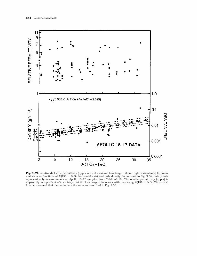
544 Lunar Sourcebook
Fig. 9.59. Relative dielectric permittivity (upper vertical axis) and loss tangent (lower right vertical axis) for lunar materials as functίons of %(TiO2 + FeO) (horizontal axis) and bulk density. In contrast to Fig. 9.56, data points represent only measurements on Apollo 15–17 samples (from Table A9.16). The relatίve permittivity (upper) is apparently independent of chemistry, but the loss tangent increases with increasing %(TiO2 + FeO). Theoretical fitted curves and their derivation are the same as described in Fig. 9.56.
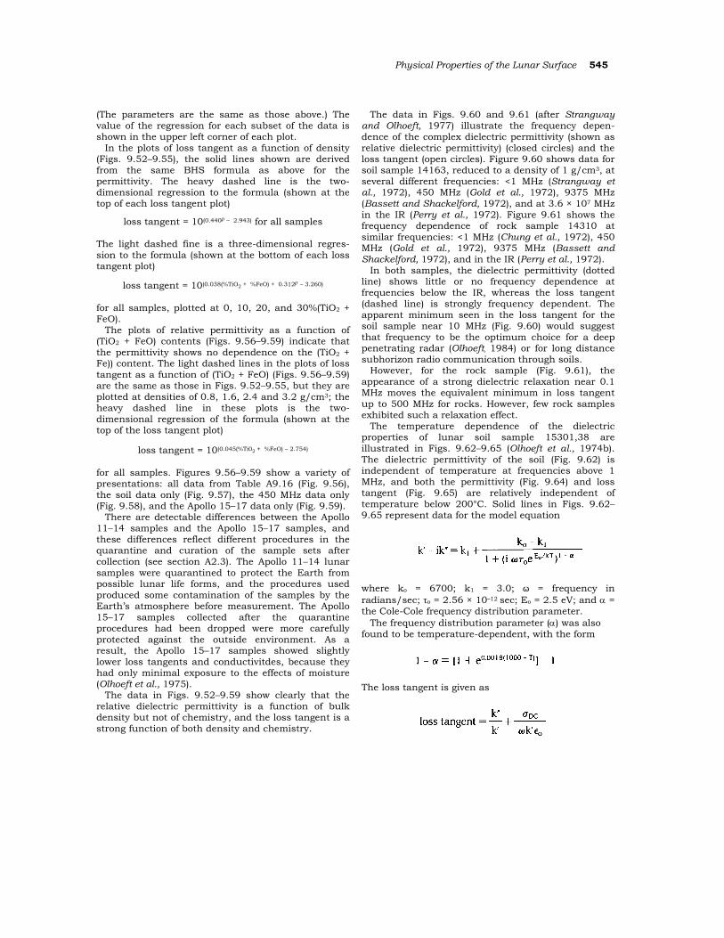
Physical Properties of the Lunar Surface 545
(The parameters are the same as those above.) The value of the regression for each subset of the data is shown in the upper left corner of each plot.
In the plots of loss tangent as a function of density (Figs. 9.52–9.55), the solid lines shown are derived from the same BHS formula as above for the permittivity. The heavy dashed line is the two-dimensional regression to the formula (shown at the top of each loss tangent plot)
loss tangent = 10(0.440ρ – 2.943) for all samples The light dashed fine is a three-dimensional regres-sion to the formula (shown at the bottom of each loss tangent plot)
loss tangent = 10(0.038(%TiO2 + %FeO) + 0.312ρ – 3.260)
for all samples, plotted at 0, 10, 20, and 30%(TiO2 + FeO).
The plots of relative permittivity as a function of (TiO2 + FeO) contents (Figs. 9.56–9.59) indicate that the permittivity shows no dependence on the (TiO2 + Fe)) content. The light dashed lines in the plots of loss tangent as a function of (TiO2 + FeO) (Figs. 9.56–9.59) are the same as those in Figs. 9.52–9.55, but they are plotted at densities of 0.8, 1.6, 2.4 and 3.2 g/cm3; the heavy dashed line in these plots is the two-dimensional regression of the formula (shown at the top of the loss tangent plot)
loss tangent = 10(0.045(%Τi02 + %FeO) – 2.754)
for all samples. Figures 9.56–9.59 show a variety of presentations: all data from Table A9.16 (Fig. 9.56), the soil data only (Fig. 9.57), the 450 MHz data only (Fig. 9.58), and the Apollo 15–17 data only (Fig. 9.59).
There are detectable differences between the Apollo 11–14 samples and the Apollo 15–17 samples, and these differences reflect different procedures in the quarantine and curation of the sample sets after collection (see section Α2.3). The Apollo 11–14 lunar samples were quarantined to protect the Earth from possible lunar life forms, and the procedures used produced some contamination of the samples by the Earth’s atmosphere before measurement. The Apollo 15–17 samples collected after the quarantine procedures had been dropped were more carefully protected against the outside environment. As a result, the Apollo 15–17 samples showed slightly lower loss tangents and conductivitdes, because they had only minimal exposure to the effects of moisture (Olhoeft et al., 1975).
The data in Figs. 9.52–9.59 show clearly that the relative dielectric permittivity is a function of bulk density but not of chemistry, and the loss tangent is a strong function of both density and chemistry.
The data in Figs. 9.60 and 9.61 (after Strangway and Olhoeft, 1977) illustrate the frequency depen-dence of the complex dielectric permittivity (shown as relative dielectric permittivity) (closed circles) and the loss tangent (open circles). Figure 9.60 shows data for soil sample 14163, reduced to a density of 1 g/cm3, at several different frequencies: <1 MHz (Strangway et al., 1972), 450 MHz (Gold et al., 1972), 9375 MHz (Bassett and Shackelford, 1972), and at 3.6 × 10⁷ MHz in the IR (Perry et al., 1972). Figure 9.61 shows the frequency dependence of rock sample 14310 at similar frequencies: <1 MHz (Chung et al., 1972), 450 MHz (Gold et al., 1972), 9375 MHz (Bassett and Shackelford, 1972), and in the IR (Perry et al., 1972).
In both samples, the dielectric permittivity (dotted line) shows little or no frequency dependence at frequencies below the IR, whereas the loss tangent (dashed line) is strongly frequency dependent. The apparent minimum seen in the loss tangent for the soil sample near 10 MHz (Fig. 9.60) would suggest that frequency to be the optimum choice for a deep penetrating radar (Olhoeft, 1984) or for long distance subhorizon radio communication through soils.
However, for the rock sample (Fig. 9.61), the appearance of a strong dielectric relaxation near 0.1 MHz moves the equivalent minimum in loss tangent up to 500 MHz for rocks. However, few rock samples exhibited such a relaxation effect.
The temperature dependence of the dielectric properties of lunar soil sample 15301,38 are illustrated in Figs. 9.62–9.65 (Olhoeft et al., 1974b). The dielectric permittivity of the soil (Fig. 9.62) is independent of temperature at frequencies above 1 MHz, and both the permittivity (Fig. 9.64) and loss tangent (Fig. 9.65) are relatively independent of temperature below 200°C. Solid lines in Figs. 9.62–9.65 represent data for the model equation
where ko = 6700; k1 = 3.0; ω = frequency in radians/sec; τo = 2.56 × 10⁻¹² sec; Eo = 2.5 eV; and α = the Cole-Cole frequency distribution parameter.
The frequency distribution parameter (α) was also found to be temperature-dependent, with the form
The loss tangent is given as
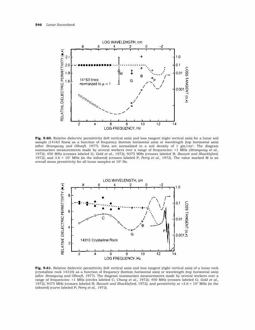
546 Lunar Sourcebook
Fig. 9.60. Relative dielectric permittivity (left vertical axis) and loss tangent (right vertical axis) for a lunar soil sample (14163 fines) as a function of frequency (bottom horizontal axis) or wavelength (top horizontal axis) (after Strangway and Olhoeft, 1977). Data are normalized to a soil density of 1 gm/cm3. The diagram summarizes measurements made by several workers over a range of frequencies: <1 MHz (Strangway et al., 1972); 450 MHz (crosses labeled G; Gold et al., 1972); 9375 MHz (crosses labeled B; Bassett and Shackleford, 1972); and 3.6 × 10⁷ MHz (in the infrared) (crosses labeled P; Perry et al., 1972). The value marked Μ is an overall mean permittivity for all lunar samples at 107 Hz.
Fig. 9.61. Relative dielectric permittivity (left vertical axis) and loss tangent (right vertical axis) of a lunar rock (crystalline rock 14310) as a function of frequency (bottom horizontal axis) or wavelength (top horizontal axis) (after Strangway and Olhoeft, 1977). The diagram summarizes measurements made by several workers over a range of frequencies: <1 MHz (circles labeled C; Chung et al., 1972); 450 MHz (crosses labeled G; Gold et al., 1972); 9375 MHz (crosses labeled B; Bassett and Shackleford, 1972); and permittivity at >3.6 × 10⁷ MHz (in the infrared) (curve labeled P; Perry et al., 1972).
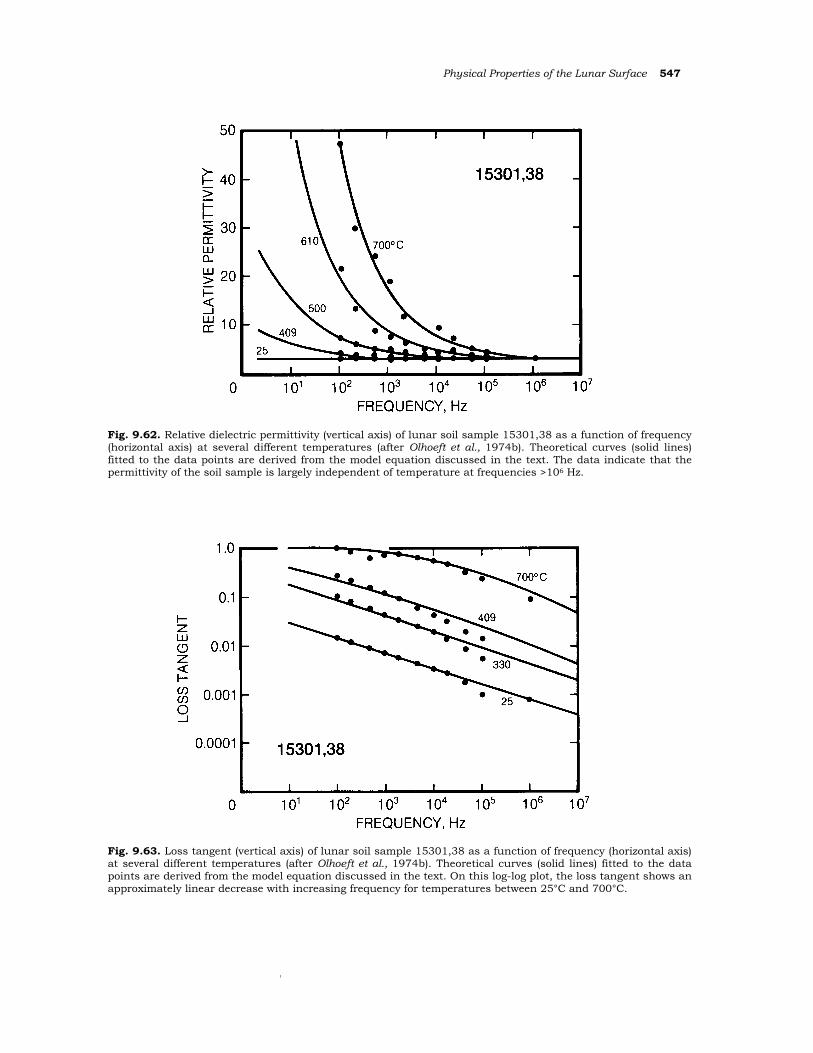
Physical Properties of the Lunar Surface 547
Fig. 9.62. Relative dielectric permittivity (vertical axis) of lunar soil sample 15301,38 as a function of frequency (horizontal axis) at several different temperatures (after Olhoeft et al., 1974b). Theoretical curves (solid lines) fitted to the data poίnts are derived from the model equation discussed in the text. The data indicate that the permittivity of the soil sample is largely independent of temperature at frequencies >106 Hz.
Fig. 9.63. Loss tangent (vertical axis) of lunar soil sample 15301,38 as a function of frequency (horizontal axis) at several different temperatures (after Olhoeft et al., 1974b). Theoretical curves (solid lines) fitted to the data points are derived from the model equation discussed in the text. On this log-log plot, the loss tangent shows an approximately linear decrease with increasing frequency for temperatures between 25°C and 700°C.
Ι
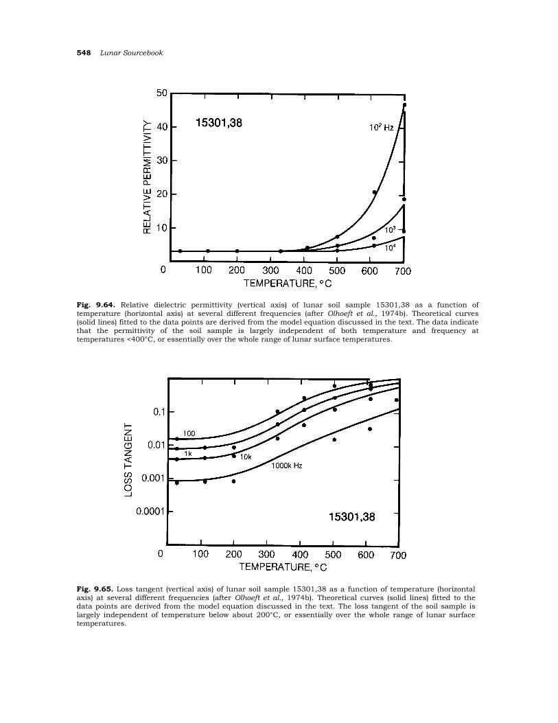
548 Lunar Sourcebook
Fig. 9.64. Relative dielectric permittivίty (vertical axis) of lunar soil sample 15301,38 as a functίon of temperature (horίzontal axis) at several different frequencies (after Olhoeft et al., 1974b). Theoretical curves (solid lines) fitted to the data points are derived from the model equation discussed in the text. The data indicate that the permittivity of the soil sample is largely independent of both temperature and frequency at temperatures <400°C, or essentially over the whole range of lunar surface temperatures.
Fig. 9.65. Loss tangent (vertical axis) of lunar soil sample 15301,38 as a function of temperature (horizontal axis) at several different frequencies (after Olhoeft et al., 1974b). Theoretical curves (solid lines) fitted to the data points are derived from the model equation discussed in the text. The loss tangent of the soil sample is largely independent of temperature below about 200°C, or essentially over the whole range of lunar surface temperatures.
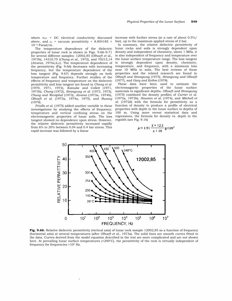
Physical Properties of the Lunar Surface 549
where σDC = DC electrical conductivity discussed above, and εo = vacuum permittivity = 8.854185 × 10⁻¹² Farad/m.
The temperature dependence of the dielectric properties of lunar rock is shown in Figs. 9.66–9.71 for several different samples: 12002,85 (Olhoeft et al., 1973b), 14310,75 (Chung et al., 1972), and 70215,14 (Alvarez, 1974a,b,c). The temperature dependence of the permittivity (Fig. 9.66) decreases with increasing frequency, but the temperature dependence of the loss tangent (Fig. 9.67) depends strongly on both temperature and frequency. Further studies of the effects of frequency and temperature on the dielectric permittivity and loss tangent are found in Chung et al. (1970, 1971, 1972), Katsube and Collett (1971, 1973b), Chung (1972), Strangway et αl. (1972, 1975), Chung and Westphal (1973), Alvarez (1973a, 1974b), Οlhοeft et al. (1973a, 1974a, 1975), and Bussey (1979).
Frisillo et al. (1975) added another variable to these investigations by studying the effects of frequency, temperature and vertical confining stress on the electromagnetic properties of lunar soils. The loss tangent showed no dependence upon stress. However, the relative dielectric permittivity increased rapidly from 6% to 20% between 0.04 and 0.4 bar stress. This rapid increase was followed by a linear
increase with further stress (at a rate of about 0.5%/ bar), up to the maximum applied stress of 2 bar.
In summary, the relative dielectric permittivity of lunar rocks and soils is strongly dependent upon density and independent of chemistry; above 1 MHz, it is also independent of frequency and temperature over the lunar surface temperature range. The loss tangent is strongly dependent upon density, chemistry, temperature, and frequency, with a minimum loss near 10 MHz in soils. The best reviews of these properties and the related research are found in Olhoeft and Strangway (1975), Strangway and Olhoeft (1977), and Gary and Keihm (1978).
These data have been used to estimate the electromagnetic properties of the lunar surface materials to significant depths. Olhoeft and Strangway (1975) combined the density profiles of Carrier et al. (1972a, 1973b), Houston et al. (1974), and Mitchell et al. (1972d) with the formula for permittivity as a function of density to produce a profile of electrical properties with depth in the lunar surface to depths of 100 m. Using more recent statistical data and regressions, the formula for density vs. depth in the regolith (see Fig. 9.16)
Fig. 9.66. Relative dielectric permittivity (vertical axis) of lunar rock sample 12002,85 as a function of frequency (horizontal axis) at several temperatures (after Olhoeft et al., 1973a). The solid lines are smooth curves fitted to the data. Curves derived from the model equation described in the text are more complicated and are not shown here. At prevailing lunar surface temperatures (<200°C), the permittivity of the rock is virtually independent of frequency for frequencies >103 Hz.
Ι
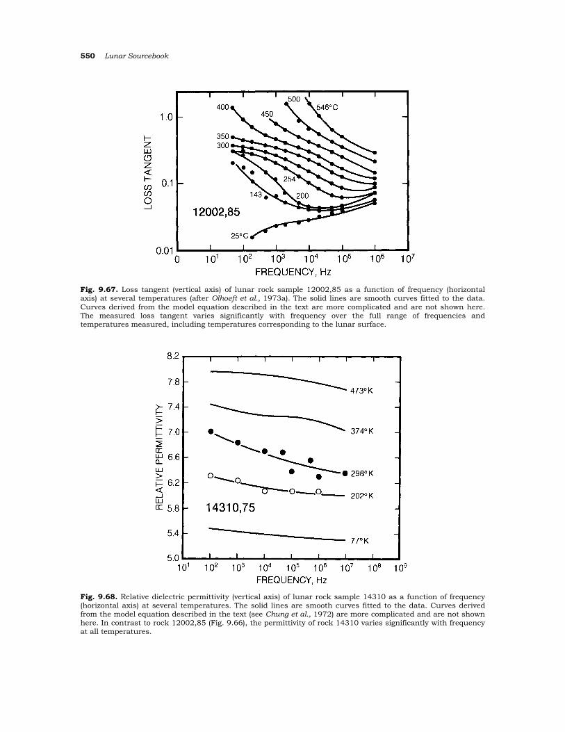
550 Lunar Sourcebook
Fig. 9.67. Loss tangent (vertical axis) of lunar rock sample 12002,85 as a function of frequency (horizontal axis) at several temperatures (after Olhoeft et al., 1973a). The solid lines are smooth curves fitted to the data. Curves derived from the model equation described in the text are more complicated and are not shown here. The measured loss tangent varies significantly with frequency over the full range of frequencies and temperatures measured, including temperatures corresponding to the lunar surface.
Fig. 9.68. Relative dielectric permittivity (vertical axis) of lunar rock sample 14310 as a function of frequency (horizontal axis) at several temperatures. The solid lines are smooth curves fitted to the data. Curves derived from the model equation described in the text (see Chung et al., 1972) are more complicated and are not shown here. In contrast to rock 12002,85 (Fig. 9.66), the permittivity of rock 14310 varies significantly with frequency at all temperatures.
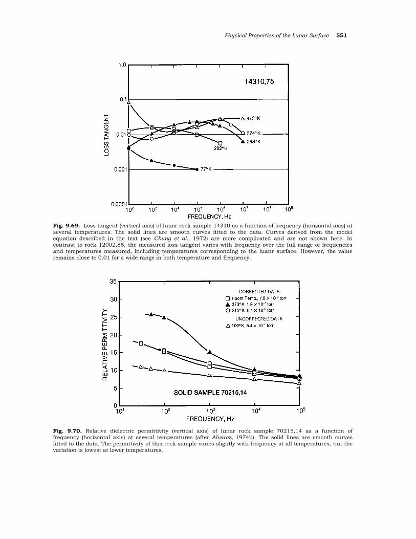
Physical Properties of the Lunar Surface 551
Fig. 9.69. Loss tangent (vertical axis) of lunar rock sample 14310 as a function of frequency (horizontal axis) at several temperatures. The solid lines are smooth curves fitted to the data. Curves derived from the model equation described in the text (see Chung et al., 1972) are more complicated and are not shown here. In contrast to rock 12002,85, the measured loss tangent varies with frequency over the full range of frequencies and temperatures measured, including temperatures corresponding to the luanr surface. However, the value remains close to 0.01 for a wide range in both temperature and frequency.
Fig. 9.70. Relative dielectric permittivity (vertical axis) of lunar rock sample 70215,14 as a function of frequency (horizontal axis) at several temperatures (after Alvarez, 1974b). The solid lines are smooth curves fitted to the data. The permittivity of this rock sample varies slightly with frequency at all temperatures, but the variation is lowest at lower temperatures.
Ι
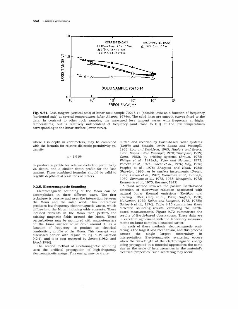
552 Lunar Sourcebook
Fig. 9.71. Loss tangent (vertical axis) of lunar rock sample 70215,14 (basaltic lava) as a function of frequency (horizontal axis) at several temperatures (after Alvarez, 1974c). The solid lines are smooth curves fitted to the data. In contrast to other rock samples, the measured loss tangent varies with frequency at higher temperatures, but is relatively independent of frequency (and close to 0.1) at the lοw temperatures corresponding to the lunar surface (lower curve).
where z is depth in centimeters, may be combined with the formula for relative dielectric permittivity vs. density
k = 1.919ρ
to produce a profile for relative dielectric permittivity vs. depth, and a similar depth profile for the loss tangent. These combined formulas should be valid to regolith depths of at least tens of meters.
9.2.5. Electromagnetic Sounding Electromagnetic sounding of the Moon can be
accomplished in three different ways. The first technique is passive and uses the interaction between the Moon and the solar wind. This interaction produces low-frequency electromagnetic waves, which diffuse into the Moon, inducing eddy currents. These induced currents in the Moon then perturb the existing magnetic fields around the Moon. These perturbations may be monitored with magnetometers on the lunar surface or in orbit around it, as a function of frequency, to produce an electrical conductivity profile of the Moon. This concept was discussed earlier with regard to Fig. 9.49 (section 9.2.1), and it is best reviewed by Sonett (1982) and Hood (1986).
The second method of electromagnetic sounding uses the artificial propagation of high-frequency electromagnetic energy. This energy may be trans-
mitted and received by Earth-based radar systems (DeWitt and Stodola, 1949; Evans and Pettengίll, 1963; Low and Davidson, 1965; Hagfors and Evans, 1968; Evans, 1969; Pettengίll, 1978; Thompson, 1979; Ostro, 1983), by orbiting systems (Brown, 1972; Phillips et al., 1973a,b; Tyler and Howard, 1973; Porcello et al., 1974; Elachί et al., 1976; May, 1976; Peeples et al., 1978; Sharpton and Head, 1982; Sharpton, 1985), or by surface instruments (Brown, 1967; Brown et al., 1967; Muhleman et al., 1968a,b, 1969; Simmons et al., 1972, 1973; Kroupenio, 1973; Kroupenio et al., 1975; Rossiter, 1977). Α third method involves the passive Earth-based
detection of microwave radiation associated with natural lunar thermal emissions (Krotikov and Troitsky, 1963; Gary et al., 1965; Hagfors, 1970; Muhleman, 1972; Keίhm and Langseth, 1973, 1975b; Schloerb et al., 1976). Table 9.16 summarizes these dielectric sounding results, excluding the Earth-based measurements. Figure 9.72 summarizes the results of Earth-based observations. These data are in excellent agreement with the laboratory measure-ments on lunar samples discussed earlier.
In each of these methods, electromagnetic scat-tering is the largest loss mechanism, and this process causes the single largest uncertainty in interpretation. Electromagnetic scattering occurs when the wavelength of the electromagnetic energy being propagated in a material approaches the same size as the scale of heterogeneities in the material’s electrical properties. Such scattering may occur
Ι
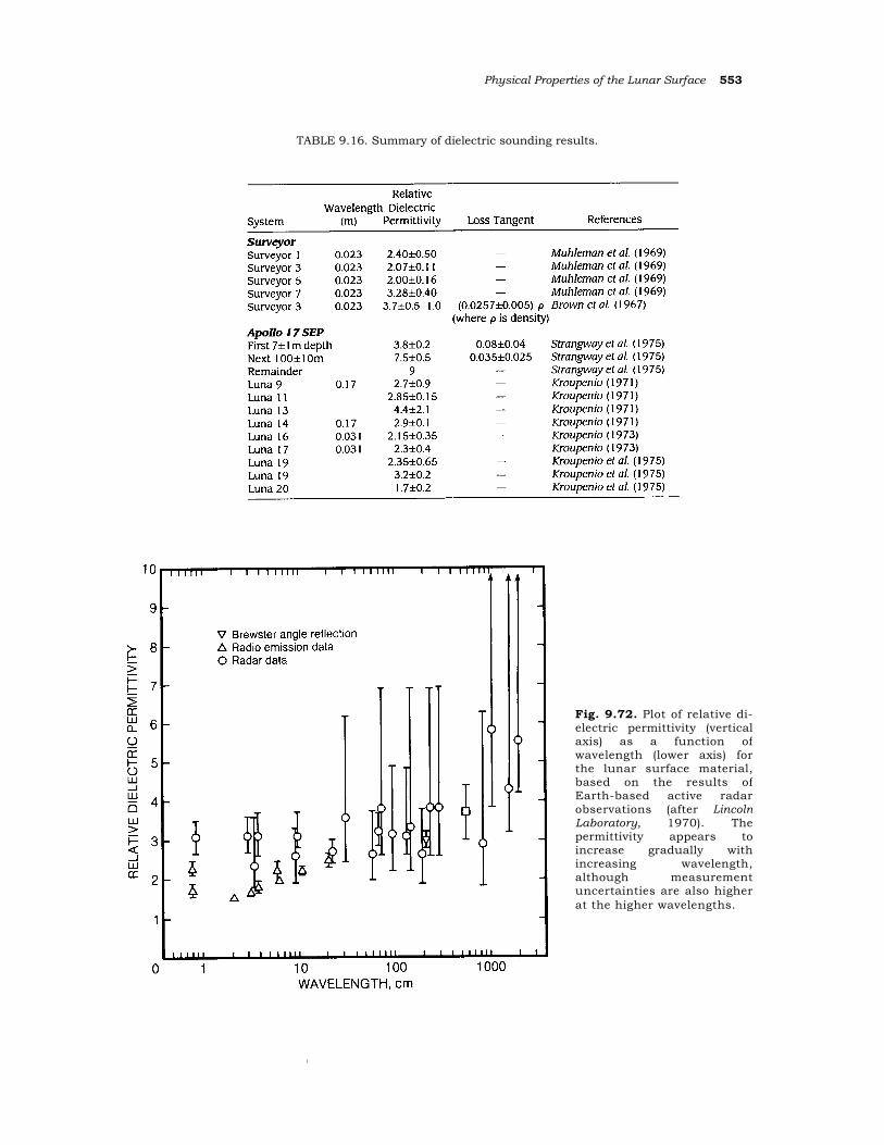
Physical Properties of the Lunar Surface 553
TABLE 9.16. Summary of dielectric sounding results.
Fig. 9.72. Plot of relative di-electric permittivity (verticalaxis) as a function ofwavelength (lower axis) forthe lunar surface material,based on the results ofEarth-based active radarobservations (after LincolnLaboratory, 1970). Thepermittivity appears toincrease gradually withincreasing wavelength,although measurementuncertainties are also higherat the higher wavelengths.
Ι
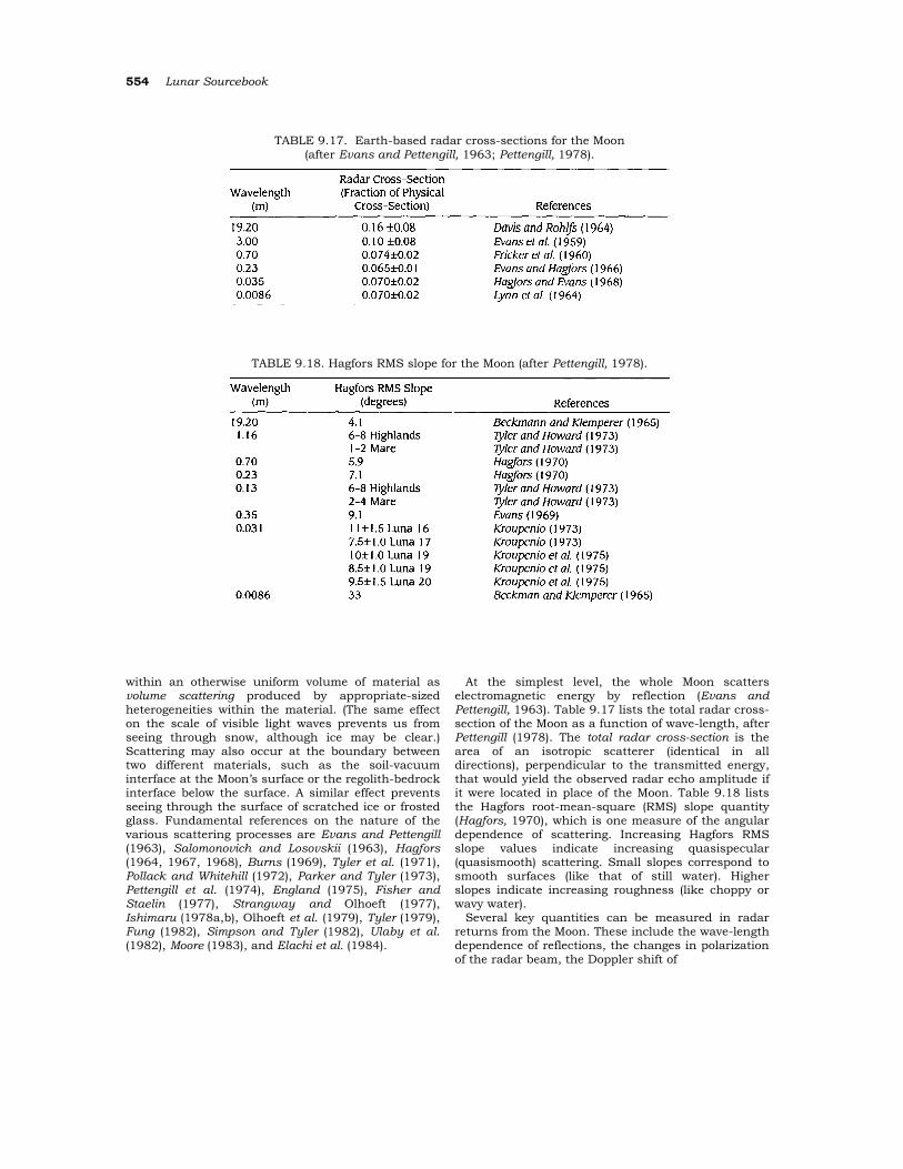
554 Lunar Sourcebook
TABLE 9.17. Earth-based radar cross-sections for the Moon (after Evans and Pettengill, 1963; Pettengill, 1978).
TABLE 9.18. Hagfors RMS slope for the Moon (after Pettengill, 1978).
within an otherwise uniform volume of material as volume scattering produced by appropriate-sized heterogeneities within the material. (The same effect on the scale of visible light waves prevents us from seeing through snow, although ice may be clear.) Scattering may also occur at the boundary between two different materials, such as the soil-vacuum interface at the Moon’s surface or the regolith-bedrock interface below the surface. Α similar effect prevents seeing through the surface of scratched ice or frosted glass. Fundamental references on the nature of the various scattering processes are Evans and Pettengill (1963), Salomonovich and Losovskii (1963), Hagfors (1964, 1967, 1968), Burns (1969), Tyler et al. (1971), Pollack and Whitehill (1972), Parker and Tyler (1973), Pettengill et al. (1974), England (1975), Fisher and Staelin (1977), Strangway and Οlhοeft (1977), Ishimaru (1978a,b), Olhoeft et al. (1979), Tyler (1979), Fung (1982), Simpson and Tyler (1982), Ulaby et al. (1982), Moore (1983), and Elachi et al. (1984).
At the simplest level, the whole Moon scatters electromagnetic energy by reflection (Evans and Pettengill, 1963). Table 9.17 lists the total radar cross-section of the Moon as a function of wave-length, after Pettengill (1978). The total radar cross-section is the area of an isotropic scatterer (identical in all directions), perpendicular to the transmitted energy, that would yield the observed radar echo amplitude if it were located in place of the Moon. Table 9.18 lists the Hagfors root-mean-square (RMS) slope quantity (Hagfors, 1970), which is one measure of the angular dependence of scattering. Increasing Hagfors RMS slope values indicate increasing quasispecular (quasismooth) scattering. Small slopes correspond to smooth surfaces (like that of still water). Higher slopes indicate increasing roughness (like choppy or wavy water).
Several key quantities can be measured in radar returns from the Moon. These include the wave-length dependence of reflections, the changes in polarization of the radar beam, the Doppler shift of
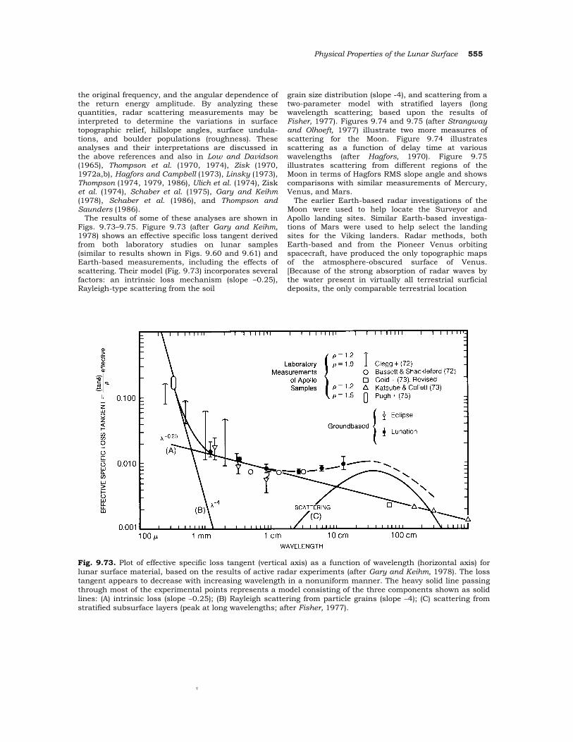
Physical Properties of the Lunar Surface 555
the original frequency, and the angular dependence of the return energy amplitude. By analyzing these quantities, radar scattering measurements may be interpreted to determine the variations in surface topographic relief, hillslope angles, surface undula-tions, and boulder populations (roughness). These analyses and their interpretations are discussed in the above references and also in Low and Davidson (1965), Thompson et al. (1970, 1974), Zisk (1970, 1972a,b), Hagfors and Campbell (1973), Linsky (1973), Thompson (1974, 1979, 1986), Ulich et al. (1974), Zisk et al. (1974), Schaber et al. (1975), Gary and Keihm (1978), Schaber et al. (1986), and Thompson and Saunders (1986).
The results of some of these analyses are shown in Figs. 9.73–9.75. Figure 9.73 (after Gary and Keihm, 1978) shows an effective specific loss tangent derived from both laboratory studies on lunar samples (similar to results shown in Figs. 9.60 and 9.61) and Earth-based measurements, including the effects of scattering. Their model (Fig. 9.73) incorporates several factors: an intrinsic loss mechanism (slope –0.25), Rayleigh-type scattering from the soil
grain size distribution (slope -4), and scattering from a two-parameter model with stratified layers (long wavelength scattering; based upon the results of Fisher, 1977). Figures 9.74 and 9.75 (after Strangway and Olhoeft, 1977) illustrate two more measures of scattering for the Moon. Figure 9.74 illustrates scattering as a function of delay time at various wavelengths (after Hagfors, 1970). Figure 9.75 illustrates scattering from different regions of the Moon in terms of Hagfors RMS slope angle and shows comparisons with similar measurements of Mercury, Venus, and Mars.
The earlier Earth-based radar investigations of the Moon were used to help locate the Surveyor and Apollo landing sites. Similar Earth-based investiga-tions of Mars were used to help select the landing sites for the Viking landers. Radar methods, both Earth-based and from the Pioneer Venus orbiting spacecraft, have produced the only topographic maps of the atmosphere-obscured surface of Venus. [Because of the strong absorption of radar waves by the water present in virtually all terrestrial surficial deposits, the only comparable terrestrial location
Fig. 9.73. Plot of effective specific loss tangent (vertical axis) as a function of wavelength (horizontal axis) for lunar surface material, based on the results of active radar experiments (after Gary and Keihm, 1978). The loss tangent appears to decrease with increasing wavelength in a nonuniform manner. The heavy solid line passing through most of the experimental points represents a model consisting of the three components shown as solid lines: (A) intrinsic loss (slope –0.25); (B) Rayleigh scattering from particle grains (slope –4); (C) scatterίng from stratified subsurface layers (peak at long wavelengths; after Fisher, 1977).
Ί
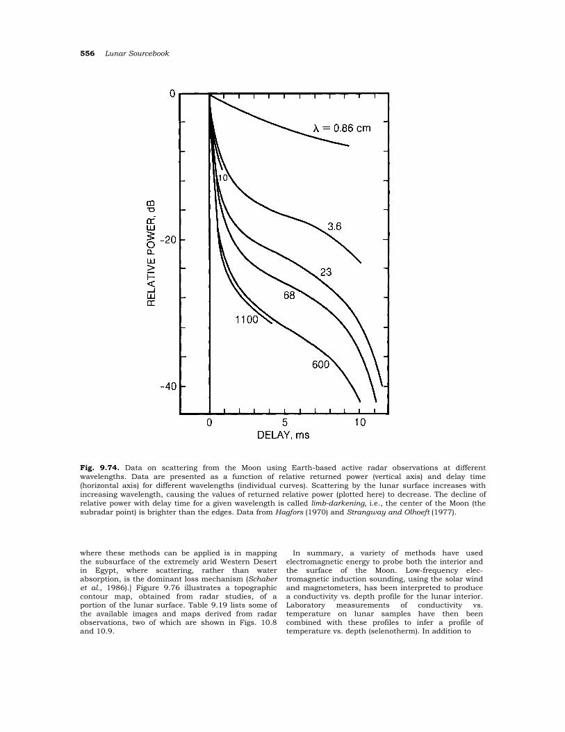
556 Lunar Sourcebook
Fig. 9.74. Data on scattering from the Moon using Earth-based active radar observations at different wavelengths. Data are presented as a function of relative returned power (vertical axis) and delay time (horizontal axis) for different wavelengths (individual curves). Scattering by the lunar surface increases with increasing wavelength, causing the values of returned relative power (plotted here) to decrease. The decline of relative power with delay time for a given wavelength is called limb-darkening, i.e., the center of the Moon (the subradar point) is brighter than the edges. Data from Hagfors (1970) and Strangway and Olhoeft (1977).
where these methods can be applied is in mapping the subsurface of the extremely arid Western Desert in Egypt, where scattering, rather than water absorption, is the dominant loss mechanism (Schaber et al., 1986).] Figure 9.76 illustrates a topographic contour map, obtained from radar studies, of a portion of the lunar surface. Table 9.19 lists some of the available images and maps derived from radar observations, two of which are shown in Figs. 10.8 and 10.9.
In summary, a variety of methods have used electromagnetic energy to probe both the interior and the surface of the Moon. Low-frequency elec-tromagnetic induction sounding, using the solar wind and magnetometers, has been interpreted to produce a conductivity vs. depth profile for the lunar interior. Laboratory measurements of conductivity vs. temperature on lunar samples have then been combined with these profiles to infer a profile of temperature vs. depth (selenotherm). In addition to
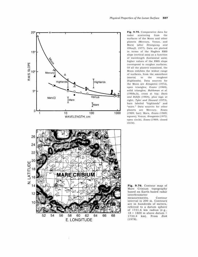
Physical Properties of the Lunar Surface 557
Fig. 9.75. Comparative data forradar scattering from thesurfaces of the Moon and otherplanets (Mercury, Venus, andMars) (after Strangway andOlhoeft, 1977). Data are plottedin terms of the Hagfors RMSslope (vertical axis) as a functionof wavelength (horizontal axis);higher values of the RMS slopecorrespond to rougher surfaces.Of all the planets examined, theMoon exhibits the widest rangeof surfaces, from the smoothest(maria) to the roughest(highlands). Data sources forthe Moon are Kroupenio (1972),open triangles; Evans (1969),solid triangles; Muhleman et al.(1968a,b), cross at top; Davisand Rohlfs (1964), plus sign atright; Tyler and Howard (1973),bars labeled “highlands” and“mare.” Data sources for otherplanets are Mercury, Evans(1969; bar); Mars, Evans (1969;square); Venus, Kroupenio (1972;open circle), Evans (1969; closedcircle).
Fig. 9.76. Contour map ofMare Crisium topographybased on Earth-based radarinterferometer measurements. Contourinterval is 200 m. Contoursare in hundreds of meters,referred to a datum sphereof 1731.6 km radius (e.g.,18 = 1800 m above datum =1733.4 km). From Zisk(1978).
Ι
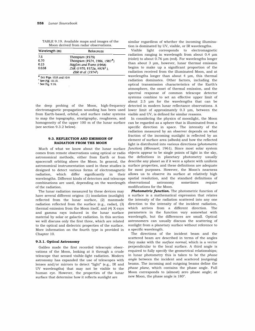
558 Lunar Sourcebook
TABLE 9.19. Available maps and images of the Moon derived from radar observations.
the deep probing of the Moon, high-frequency electromagnetic propagation sounding has been used from Earth-based, orbital, and surface radar systems to map the topography, stratigraphy, roughness, and homogeneity of the upper 100 m of the lunar surface (see section 9.3.2 below).
9.3. REFLECTION AND EMISSION OF RADIATION FROM THE MOON
Much of what we know about the lunar surface comes from remote observations using optical or radio astronomical methods, either from Earth or from spacecraft orbiting above the Moon. In general, the astronomical instrumentation used in these studies is designed to detect various forms of electromagnetic radiation, which differ significantly in their wavelengths. Different kinds of detectors and telescope combinations are used, depending on the wavelength of the radiation.
The lunar radiation measured by these devices may have several different origins: (1) insolation (sunlight) reflected from the lunar surface, (2) manmade radiation reflected from the surface (e.g., radar), (3) thermal emission from the Moon itself, and (4) X-rays and gamma rays induced in the lunar surface material by solar or galactic radiation. In this section we will discuss only the first three, which are related to the optical and dielectric properties of the surface. More information on the fourth type is provided in Chapter 10.
9.3.1. Optical Astronomy Galileo made the first recorded telescopic obser-
vations of the Moon, looking at it through a crude telescope that sensed visible-light radiation. Modern astronomy has expanded the use of telescopes with lenses and/or mirrors to detect “light” (e.g., IR and UV wavelengths) that may not be visible to the human eye. However, the properties of the lunar surface that determine how it reflects sunlight are
similar regardless of whether the incoming illumina-tion is dominated by UV, visible, or IR wavelengths.
Visible light corresponds to electromagnetic radiation ranging in wavelength from about 0.4 µm (violet) to about 0.76 µm (red). For wavelengths longer than about 3 µm, however, lunar thermal emission begins to make up a significant proportion of the radiation received from the illuminated Moon, and at wavelengths longer than about 4 µm, this thermal radiation dominates. Other factors, including the optical transmission characteristics of the Earth’s atmosphere, the onset of thermal emission, and the spectral response of common telescope detector systems combine to set an effective upper limit of about 2.5 µm for the wavelengths that can be detected in modern lunar reflectance observations. Α lower limit of approximately 0.3 µm, between the visible and UV, is defined for similar reasons.
In considering the physics of moonlight, the Moon can be regarded as a sphere that is illuminated from a specific direction in space. The intensity of the radiation measured by an observer depends on what fraction of the incoming sunlight is reflected by an element of surface area (albedo) and how the reflected light is distributed into various directions (photometric function) (Minnaert, 1961). Since most solar system objects appear to be single points of light in the sky, the definitions in planetary photometry usually describe any planet as if it were a sphere with uniform surface properties, and these definitions are adequate for most purposes. However, the Moon’s nearness allows us to observe its surface at relatively high spatial resolution, and the standard definitions of observational astronomy sometimes require modifιcations for the Moon.
Photometric function. The photometric function of a surface is a mathematical expression that relates the intensity of the radiation scattered into any one direction to the intensity of the incident radiation, which arrives from a different direction. The parameters in the function vαry somewhat with wavelength, but the differences are small. Optical astronomers can usually discuss the scattering of sunlight from a planetary surface without reference to a specific wavelength.
The directions of the incident beam and the scattered beam are described in terms of the angles they make with the surface normal, which is a vector perpendicular to the local surface. Α third angle is required to fully specify the geometrical relationships; in lunar photometry this is taken to be the phase angle between the incident and scattered (outgoing) beams. The incoming and outgoing beams define the phase plane, which contains the phase angle. Full Moon corresponds to (almost) zero phase angle; at new Moon, the phase angle is 180°.
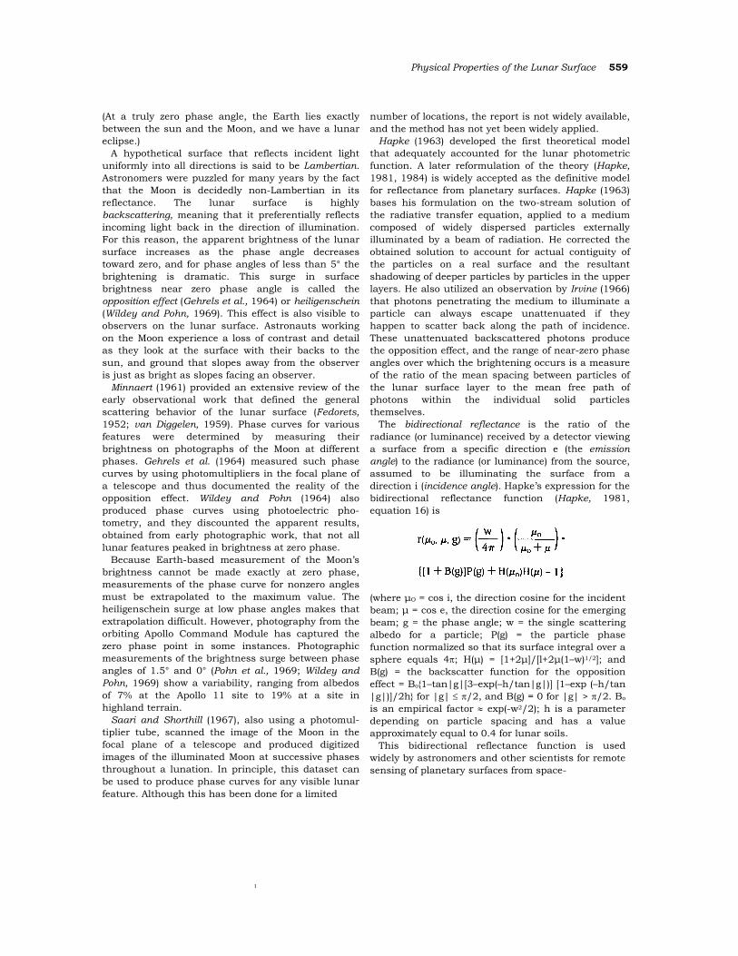
Physical Properties of the Lunar Surface 559
(At a truly zero phase angle, the Earth lies exactly between the sun and the Moon, and we have a lunar eclipse.)
A hypothetical surface that reflects incident light uniformly into all directions is said to be Lambertian. Astronomers were puzzled for many years by the fact that the Moon is decidedly non-Lambertian in its reflectance. The lunar surface is highly backscatterίng, meaning that it preferentially reflects incoming light back in the direction of illumination. For this reason, the apparent brightness of the lunar surface increases as the phase angle decreases toward zero, and for phase angles of less than 5° the brightening is dramatic. This surge in surface brightness near zero phase angle is called the oppositίon effect (Gehrels et al., 1964) or heiligenschein (Wildey and Pohn, 1969). This effect is also visible to observers on the lunar surface. Astronauts working on the Moon experience a loss of contrast and detail as they look at the surface with their backs to the sun, and ground that slopes away from the observer is just as bright as slopes facing an observer.
Minnaert (1961) provided an extensive review of the early observational work that defined the general scattering behavior of the lunar surface (Fedorets, 1952; van Diggelen, 1959). Phase curves for various features were determined by measuring their brightness on photographs of the Moon at different phases. Gehrels et al. (1964) measured such phase curves by using photomultipliers in the focal plane of a telescope and thus documented the reality of the opposition effect. Wildey and Pohn (1964) also produced phase curves using photoelectric pho-tometry, and they discounted the apparent results, obtained from early photographic work, that not all lunar features peaked in brightness at zero phase.
Because Earth-based measurement of the Moon’s brightness cannot be made exactly at zero phase, measurements of the phase curve for nonzero angles must be extrapolated to the maximum value. The heiligenschein surge at lοw phase angles makes that extrapolation difficult. However, photography from the orbiting Apollo Command Module has captured the zero phase point in some instances. Photographic measurements of the brightness surge between phase angles of 1.5° and 0° (Pohn et al., 1969; Wildey and Pohn, 1969) show a variability, ranging from albedos of 7% at the Apollo 11 site to 19% at a site in highland terrain.
Saari and Shorthill (1967), also using a photomul-tiplier tube, scanned the image of the Moon in the focal plane of a telescope and produced digitized images of the illuminated Moon at successive phases throughout a lunation. In principle, this dataset can be used to produce phase curves for any visible lunar feature. Although this has been done for a limited
number of locations, the report is not widely available, and the method has not yet been widely applied.
Hapke (1963) developed the first theoretical model that adequately accounted for the lunar photometric function. A later reformulation of the theory (Hapke, 1981, 1984) is widely accepted as the definitive model for reflectance from planetary surfaces. Hapke (1963) bases his formulation on the two-stream solution of the radiative transfer equation, applied to a medium composed of widely dispersed particles externally illuminated by a beam of radiation. He corrected the obtained solution to account for actual contiguity of the particles on a real surface and the resultant shadowing of deeper particles by particles in the upper layers. He also utilized an observation by Irvine (1966) that photons penetrating the medium to illuminate a particle can always escape unattenuated if they happen to scatter back along the path of incidence. These unattenuated backscattered photons produce the opposition effect, and the range of near-zero phase angles over which the brightening occurs is a measure of the ratio of the mean spacing between particles of the lunar surface layer to the mean free path of photons within the individual solid particles themselves.
The bidirectional reflectance is the ratio of the radiance (or luminance) received by a detector viewing a surface from a specific direction e (the emission angle) to the radiance (or luminance) from the source, assumed to be illuminating the surface from a direction i (incidence angle). Hapke’s expression for the bidirectional reflectance function (Hapke, 1981, equation 16) is
(where µO = cos i, the direction cosine for the incident beam; µ = cos e, the direction cosine for the emerging beam; g = the phase angle; w = the single scattering albedo for a particle; P(g) = the particle phase function normalized so that its surface integral over a sphere equals 4π; Η(µ) = [1+2µ]/[l+2µ(1–w)1/2]; and B(g) = the backscatter function for the opposition effect = Bo{1–tan|g|[3–exp(–h/tan|g|)] [1–exp (–h/tan |g|)]/2h} for |g| ≤ π/2, and B(g) = 0 for |g| > π/2. Bo is an empirical factor ≈ exp(-w2/2); h is a parameter depending on particle spacing and has a value approximately equal to 0.4 for lunar soils.
This bidirectional reflectance function is used widely by astronomers and other scientists for remote sensing of planetary surfaces from space-
Ι
560 Lunar Sourcebook
craft. For such observations, the resolution element on the planetary surface can range from tens of meters to several kilometers across. The terrain may contain craters, mounds, and other topographic features that cause the direction of the local surface normal to vary within a single resolution element. When this happens, local angles of incidence and emission will also vary. When i > π/2, an area will lie in shadow; when e > π/2, an area will be on the backside of a slope and invisible to the observer. In addition, one feature may block the view of another. All these conditions associated with macroscopic roughness lead to errors in the predictions of the model. The errors are particularly large when astronomers observe the limb regions of a planet or when spacecraft sensors point to surface regions lying near the horizon.
Hapke (1984) derived an expression for correcting any photometric function for the effects of roughness. The correction works quite well, as he demonstrated. Application of the correction is not difficult, but the explanation is too lengthy to reproduce here. The interested reader will find it discussed in detail in the original paper.
Albedo. The spherical albedo or Bond albedo is the fraction of sunlight reflected by a planet in all directions. For the Moon, the actual value will depend on which side is illuminated. The values discussed here refer to the Earth-facing hemisphere, or nearside, which contains most of the dark maria.
The Bond albedo of a planet is difficult to measure, and astronomers historically have derived it from measurements of a related quantity, the geometrical albedo (p). The geometrical albedo is the ratio of the radiance from a planet at zero phase (e.g., full Moon) to that of a perfectly diffusing planar surface (Lambert reflector) located at the same distance from the sun and normal to the incident radiation (Kaula, 1968, p. 260). The geometrical albedo is related to the spherical (Bond) albedo (A) by the simple relationship A = pq, where q, the phase integral, is given by
The phase angle g is the angle between the sun and the Earth as seen from the planet, and the phase function φ describes the variation of brightness of a planet over the range of possible phase angles. The value of the phase integral can be obtained by calculating the area under the phase curve, the plot of φ(g). For the Moon the function φ can be derived from the Hapke photometric function. Values quoted in the literature for the phase integral are derived from Earth-based measurements of moonlight.
Finally, the reflectance of a surface element viewed normally (i.e., along the surface normal) at zero phase angle relative to the ideal white diffusing plate is called the normal albedo (Minnaert, 1961, p. 218). When the angles i = e = 0 are substituted into Hapke’s formula, the result is the normal albedo. The value of the normal albedo for an area of lunar surface will depend on the local chemical and mineralogical composition, particle size, packing density, etc. In general, crater ray systems are the brightest features on the Moon, and highland areas are brighter than maria.
For lunar surface materials, the brightness of any area, observed from the Earth at full Moon (zero phase), yields a value that is virtually that of the normal albedo for that area, irrespective of the orientation of the surface normal to the direction of illumination. However, the formal definition of normal albedo requires the surface element to be illuminated normally.
Maps of the Moon showing the normal albedo of surface features have been produced by Pohn and Wildey (1970) and Wildey (1978). The earlier map is based on a carefully calibrated full Moon photograph (phase angle = 1.5°) that was digitized by a scanning microdensitometer. The resulting contours of equal film density were converted to radiance using photoelectric observations of a network of lunar surface features, taken at the same time as the photographic exposure. However, as discussed earlier, no photograph of the Moon from Earth can exhibit exact zero phase, and these studies therefore do not rigorously provide the true normal albedo of lunar features.
In the later work, Wildey (1978) digitized a series of photographs taken over a range of phase angles between 2.5° and 4.0°. By fitting a parametric function to the data as a function of phase, he was able to extrapolate to develop a lunar “image” of ideal normal albedo as well as a corollary image representing the magnitude of the heiligenschein effect across the nearside of the Moon.
The mapping of lunar surface brightness during a lunation (Saari and Shorthill, 1967) included an image taken at a phase angle of –2°, which is, in essence, a map of normal albedo. The data were collected using a photomultiplier to scan the lunar image in the focal plane of the telescope.
Dollfus and Bowell (1971) studied measurements of normal albedo in 9 different reports and derived a best estimate of this quantity for 67 lunar regions; the albedo for these regions ranges from 5.7% to 18.4%.
Single scattering albedo. Modern formulations of reflectance from planetary surfaces are based on the concepts of radiative transfer theory (e.g., Hapke,
Physical Properties of the Lunar Surface 561
1981). The fundamental transport equation invokes a hypothetical volume element within the surface that, when illuminated by a pencil of radiation from an arbitrary direction, absorbs a fraction of it and scatters the remainder in various directions relative to the incident direction. The fraction absorbed (absorption coefficient), the fraction scattered (scattering coefficient), and the distribution function for the scattered component are all parameters in the solution to the transport equation. The single scattering albedo is the ratio of the scattering coefficient to the sum of the scattering and absorption coefficients.
In the Mie theory, scattering and absorbing particles are ideal dielectric spheres. In such a situation, the single scattering albedo is related to the physical properties of the material and the size of the particles relative to the wavelength of the radiation. The derivation of the basic radiative transport equation further assumes that the scattering centers in the medium are well separated so that they interact independently with the radiation field. Although the more complicated structure of a real planetary surface violates these assumptions, the Mie theory works well within the limits of various approximations that must be applied to the real problems.
Unfortunately, the considerable unreality of these same approximations blurs the physical meaning of the single scattering albedo values that are derived from applying the theory to actual reflectance measurements. For example, values obtained by fitting Hapke’s (1981) function to phase curves for lunar regions can be used only for intercomparison with other lunar or planetary data or with laboratory measurements on lunar soils and analogue materials.
Polarization. Sunlight is unpolarized. In other words, the oscillations of the electric and magnetic vectors of the light waves in sunlight are not preferentially aligned in any particular direction. If sunlight is transmitted through a polarizer, its intensity after transmission does not depend on the rotation angle of the polarizer.
If sunlight is reflected from a smooth surface in some direction other than back along the surface normal, the reflected light becomes at least partially plane polarized. (This is a familiar phenomenon associated with Fresnel reflection, and it explains why polaroid sunglasses are effective in reducing glare.)
The polarization of the reflected light is specified by two quantities: the percentage of the intensity attributable to the polarized component and the angle that the direction of the electric vector makes with the normal to the phase plane, i.e., the plane
that contains the incoming and reflected light rays. These quantities are called the degree of polarization and the azimuth of polarization, respectively.
Although the lunar surface is far from smooth at the dimensions (~0.4–1.0 µm) equivalent to optical wavelengths, moonlight nevertheless is partially polarized. The degree of polarization (P) is given by the relation
where I1 is the intensity observed normal to the phase plane, and I2 is the intensity parallel to it (Dollfus, 1961). If P is positive the azimuth is assumed to be 180°, while a negative value of P implies an azimuth of 90°. These simple definitions suffice for lunar polarimetry because Lyot (1929) discovered that the polarization of moonlight is coincident with the phase plane near full Moon, disappears around phase 23°, and then grows in magnitude but rotated 90°, perpendicular to the phase plane. Similarly, Gehrels et al. (1964) failed to find any gradual rotation of the plane of polarization; the polarization vector either lies within or normal to the phase plane. They also observed that the positive maximum in polarization of reflected light from the lunar surface was highest in the UV (0.36 µm), intermediate in the green (0.54 µm), and lowest in the near IR (0.94 µm).
Dollfus and Bowell (1971) reviewed and discussed lunar polarization observations, presented new data, and elucidated the details of the polarization mechanism. For example, at a given wavelength, the negative branch of the curve, corresponding to phases of 0 ≤ g <~ 23°, has approximately the same form for all lunar terrains. Similarly, the minimum value of the negative branch, Pmin, remains constant for all lunar regions, but it decreases from –10‰ (–10 parts per thousand) at a wavelength λ = 0.325 µm to –12‰ at λ = 1.050 µm. The average value for all wavelengths is Pmin = 11.2 ± 0.3‰ and g(Pmin) = 9.6 ± 0.6°.
On the positive branch of the polarization curve, corresponding to phases >~ 23°, the maximum value of polarization (Pm) varies inversely with the albedo of the lunar terrain. The highest value noted for Pm is 350‰ for a dark mare region in Oceanus Procellarum at λ = 0.325 µm. However, regions of high albedo, such as highlands or young rayed craters, can display Pm values as low as 30‰, a value measured at Aristarchus at λ = 0.6 µm. The phase angle of maximum polarization, g(Pm), increases with Pm, but the correlation is independent of wavelength. This relation can be expressed by the equation
562 Lunar Sourcebook
where g(Pm) ίs expressed in degrees and Pm in thousandths. Dollfus and Bowell (1971) note that uniform behavior of polarization across the entίre observable lunar dίsk provides strong evidence that the properties of the microstructure of the upper lunar surface are remarkably uniform all across the Moon.
A fascίnating correlation between the polarίzation maximum (Pm) and the normal albedo (λ) has also been dίscovered. The relation is given by
A similar relationship between geometric albedo (q) and the slope of the polarization curve at the inversion point has also been documented in later work (Zellner et al., 1977). This latter correlation has proved to be particularly important in the determination of albedos of asteroids and other small bodies in the solar system. Based on both lunar sample measurements and lunar observations (Bowell et al., 1973), the best-fit relation for the Moon is
where p is the geometric albedo for a lunar region and h is the inversion slope given in percent per degree. This relation is also consistent with one derived by Veverka and Noland (1973) from lunar data published by Dollfus and Bowell (1971) and Dollfus et al. (1971).
9.3.2. Radar Astronomy
Powerful radar installations built for military purposes during World War II were subsequently utilized in the postwar period to detect echoes reflected from the Moon. The first successful attempts in 1946 produced only marginal returned signals (DeWitt and Stodola, 1949), but rapid improvements in the technology soon made possίble accurate ranging to the Moon, measurements of the Doppler shifts produced by lunar motions, the detection of Faraday rotation of the polarίzation vector of the signals in the Earth’s ionosphere, the determination of the gross radar scattering law for the lunar surface, and estimates of the Moon’s radar cross-section (Evans, 1962).
The transmitted radio signal can be pictured as a plane wave traveling from the antenna and striking the Moon. If the Moon behaves like a smooth dielectric sphere, the plane wave will strike it first at the point closest to the antenna—the subradar point. The only energy reflected back to the antenna would come from a small zone surrounding the subradar point, corresponding to the area of the first Fresnel zone of the wavefront. The remainder of the
incoming energy would be scattered by the rest of the Moon and would travel in other directions, according to the laws of specular reflection.
Most of the returned energy is observed to come from an area surrounding the subradar point. However, definite radar echoes can be detected from regions out to the lunar limb, implying that the lunar surface is not entirely smooth at radar wavelengths. For these reasons, radar reflection from the Moon is commonly described as “quasispecular,” because the strong central reflection only approximates the expected behavior of an ideally smooth spherical mirror.
Radar backscattering. The brightness (cross-section) of the subradar point is a measure of the dielectric constant of the lunar surface, while the shape of the trailing echo (scattering function) is a measure of the surface roughness and heterogeneity of the surface on the scale of the wavelength being used. The radar echo from the zone immediately around the subradar point is approximately three orders of magnitude stronger than the echo from the annular region at the lunar limb (Thompson, 1979).
Radar systems have the capability to transmit energy with a single mode of polarization and then to detect and analyze the returned energy in both the originally transmitted mode of polarίzation and the orthogonal mode. Commonly the transmitted signal is circularly polarized to minimize the effects of Faraday rotation during the signal’s outward passage through the Earth’s ionosphere. The process of reflection from an ideal dielectric sphere reverses the direction of circular polarίzation. When lunar radar observations are made, the energy returned with the direction of polarization to be expected from an ideal sphere is called polarized; the energy received in the other direction of polarization is called depolarized. A nonspecular component is also present in the polarized return; this component is qualitatively attributed to flat surfaces that happen to be tilted toward the radar. The depolarized return is attributed to the presence of surface rocks and surface roughness. Radar energy can penetrate a distance of 10 to 50 wavelengths into the extremely dry lunar regolith, allowing subsurface rocks, possibly as deep as several meters, to contribute to the radar reflections returned to Earth.
Although the strengths of the polarized and depolarized returns (echoes) are quite different near the subradar point, the falloff in the strengths of the two types of returns toward the limb regions exhibits somewhat similar behavior (Hagfors, 1967). Near the subradar point, the polarized echoes are quite strong, and they decrease sharply and nonunίformly with increasing angle of incidence from the subradar point (i = 0°) outward to about i = 35°. From about
Physical Properties of the Lunar Surface 563
i = 35° outward, the slope of the angular dependence becomes more gradual, varyίng as cos3/2i out to approximately i = 80° (Evans and Hagfors, 1966). Beyond i = 80° to the limb (0 = 90°), the dependence is proportional to cos i. In contrast, the strength of the depolarized echo varίes uniformly as cos i from the subradar point outward.
Although the lunar radar backscattering law is similar in form at all wavelengths, the fraction of power in the diffusely scattered component varies considerably, being much greater at higher frequencies (Hagfors, 1970). As a result, the lunar disk appears more uniformly bright when illuminated by the shorter radar wavelengths. Pettengill (discussion following Hagfors, 1970) points out that a plot comparing the lunar scattering laws is misleading when the plots are normalized to unity at the subradar point. Rather, it is more meaningful to scale the areas of the curves to be proportional to the total radar cross-sections at the corresponding wavelengths.
The form of the scattering law that is most widely used for studying the Moon and the inner planets is (Ostro, 1983)
where σo is radar cross-section per unit area, φ is the angle of incidence, ρ is the Fresnel normal-incidence power reflection, and βrms is the root-mean-square surface slope at wavelength-dependent scales. The theoretical basis for this model can be found in Hagfors (1964, 1970).
Radar cross-section. To understand the radar signal returned from the Moon, we use the basic radar equation that says
Received Power = Transmitted Power Density at the Moon × Backscatter Cross-Section of the Moon ×
Geometrical Attenuation on Return Path × Effective Antenna Aperture
For a transmitter of power Pt, the power density at the distance of the Moon, R, is given by ΡtG/4πR2. The denominator of this expression is just the geometrical attenuation due to the familiar inverse-square law, and the antenna gain G can be related to the effective antenna aperture A by
where λ is the wavelength of observation. Combining these terms, we get an expressίon for received echo power Ρr (Ostro, 1983)
where σ is the radar cross-section of the Moon. The radar cross-section σ has the dimensions of an
area and is defined as the geometrical cross-section of a metallic sphere whose radar echo has the same strength as the Moon. We can relate this quantity to the physical parameters of the Moon by considering the Moon as an absorbing dielectric sphere of radius a. Following a derivation presented by Bohren and Huffman (1983, p. 120), we can write
where ρ is the Fresnel reflection coefficient of the dielectric material (Evans and Hagfors, 1964) and g is a gain factor equal to unity for our ideal sphere. Because the Moon is not ideally smooth, some of the returned signal comes from reflections outside the small region surrounding the subradar point. (This is the diffuse component of the polarized return.) Because the lunar surface is not perfectly absorbing, some of the returned echo comes from scattering within the surface. (This is the depolarized component.) For these reasons, g is larger than unity by some unknown amount.
The product gρ can be derived directly from observational data. If the gain factor can be independently calculated, then the dielectric constant (ε) of the lunar surface can be obtained from the relation
Attempts to calculate (Rea et al., 1964, 1965) or estimate (Evans and Hagfors, 1964) the gain factor have resulted in estimates of the dielectric constant, ε, given by Hagfors (1970). Further complications can be introduced into these calculations by assuming that the surface consists of layers with differing dielectric properties or that the dielectric properties vary smoothly with depth in some way (Hagfors, 1970), both of which assumptions are more apt to be more realistic representations of the actual lunar surface.
Bistatic radar observations. When spacecraft were placed into orbit about the Moon, it became possible to carry out bistatic radar experiments in which the transmitting and receiving antennas are in different places. In the lunar experiments, antennas on Earth could detect both the direct radio or radar transmissions from the spacecraft and the nearly simultaneous reflections of the signals from the lunar surface toward Earth. A small Doppler shift in the reflection wavelength relative to the transmissiοn wavelength allows the two signals to be differentiated. The orbital motion of the radar-
564 Lunar Sourcebook
sounding spacecraft causes the point of specular reflection to move across the lunar surface along the ground track. Careful measurement of the intensity and polarization of the returned signals yields information on the reflectivity of the lunar material, possible subsurface layering, and surface slopes (Tyler, 1968b).
The effective surface resolution element in these experiments corresponds to the first Fresnel zone associated with the quasispecular reflection. The size of this zone depends on the altitude of the spacecraft as well as on the surface slope distribution. For measurements made using Explorer 35 in 1967, the surface resolution was approximately 100 km (Tyler, 1968a). For the Apollo 14 and 15 experiments, the resolution elements varied from 10 to 40 km, depending on the nature of terrain overflown (Tyler and Howard, 1973).
During a pass over Oceanus Procellarum, the transmitted signal from Explorer 35 was maintained with its linear polarization lying approximately in the plane of incidence. A Brewster null in the reflected signal was observed at an angle of incidence of 60° ± 1°, a result corresponding to a dielectric constant of 3.0 ± 0.2 at a wavelength of 2.2 m (Tyler, 1968a). This measurement was made in mare material located north-northwest of Hansteen Crater, and the result corresponds to the dielectric properties of the surface material averaged over a depth of roughly λ/8 (25 cm). The reflectivity along groundtracks in Oceanus Procellarum showed quite reproducible enhancements of approximately 30% in echo intensity for mare regions compared to highland areas (Tyler, 1968b). These differences in reflectivity can be explained either by variations in the packing fraction of the regolith or by variations in its depth. The latter explanation appears more physically realistic if one also takes into account the results of Earth-based observations.
The Apollo 14 and 15 missions provided the opportunity to continue bistatic radar investigations at wavelengths of 13 cm and 116 cm (Tyler and Howard, 1973). The signal-to-noise ratio and the surface resolution of these measurements were both an order of magnitude better than previous exper-iments of the same type. Although the extent of the datasets obtained was limited, the investigators found regions of the lunar surface whose physical properties could not easily be explained by simple models.
For λ = 13 cm, mare surfaces could be modeled well using a value of the dielectric constant ε = 3.1, with few deviations observed. At λ = 116 cm, much of the mare could also be modeled simply with a similar dielectric constant, but in this case, considerable deviations from the simple characterization
were observed. No successful models for the structure and properties of the anomalous regions could be developed; the authors speculated that their data implied the existence of some frequency dispersive mechanism, such as layering in a high-loss dielectric medium.
In highland regions the longer wavelength (116 cm) data were fitted successfully to a model using a uniform dielectric interface with ε = 2.8, a lower value for dielectric constant than that found in the maria. Observations at the shorter wavelength (13 cm) in the Apennine Mountains and in the central highland regions also yielded consistent results, but the data from units in the Palus Somni area and the rim of Mare Crisium could not be fitted with simple models at λ = 13 cm.
Since the polarization of returned radio signals can be determined, the echoes from the lunar surface also contain information about slopes and surface roughness. The complexity of both the surface and the physical mechanisms that alter the polarization of the signal permit only some general statements with any degree of confidence. In general, slopes in the highlands are higher than slopes in the maria. At λ = 13 cm, highland rms (root-mean-square) slopes range from 6° to 8°, while mare rms slopes range from 2° to 4° (Tyler and Howard, 1973). Although values derived from the 116-cm observations agree with the 13-cm data in the highlands, the mare values are only half as large as those derived from the 13-cm data. Apparently, small-scale roughness is larger in the maria.
Little work has yet been done on the lunar surface itself to verify the surface structures inferred from radar scattering behavior. A more technical discus-sion of these issues is found in Tyler (1979).
Apollo Lunar Sounder Experiment (ALSE). The ALSE was a three-channel, synthetic-aperture, orbital radar experiment operated during three orbits of the Apollo 17 mission to infer subsurface electrical conductivity structure, to profile lunar surface topographic variations, and to image the surface along the spacecraft ground track (Phillips et al., 1973a,b). In this experiment, a continuous series of short bursts of radar energy at three frequencies (5, 15, and 150 MHz) was directed from an instrument on the spacecraft toward the lunar surface, and the reflections, received by the same instrument, were measured in terms of intensity, time of arrival, and phase. The very low electrical loss characteristics of the lunar regolith permitted detection of echoes from subsurface features as well as from the surface itself.
Reduction of the ALSE data has been a very complex process, and analysis of the information has been hampered by two fundamental problems (Sharpton et al., 1984). First, the relatively weak
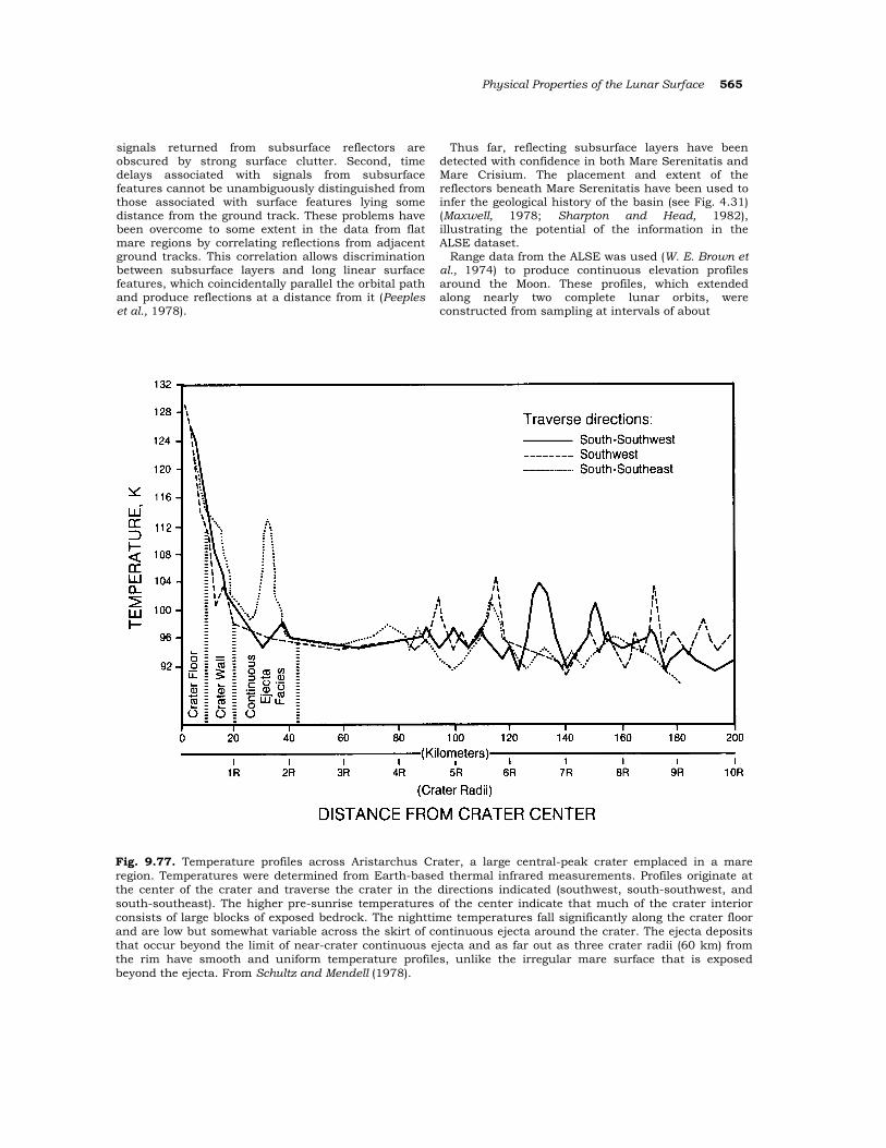
Physical Properties of the Lunar Surface 565
signals returned from subsurface reflectors are obscured by strong surface clutter. Second, time delays associated with signals from subsurface features cannot be unambiguously distinguished from those associated with surface features lying some distance from the ground track. These problems have been overcome to some extent in the data from flat mare regions by correlating reflections from adjacent ground tracks. This correlation allows discrimination between subsurface layers and long linear surface features, which coincidentally parallel the orbital path and produce reflections at a distance from it (Peeples et al., 1978).
Thus far, reflecting subsurface layers have been detected with confidence in both Mare Serenitatis and Mare Crisium. The placement and extent of the reflectors beneath Mare Serenitatis have been used to infer the geological history of the basin (see Fig. 4.31) (Maxwell, 1978; Sharpton and Head, 1982), illustrating the potential of the information in the ALSE dataset.
Range data from the ALSE was used (W. E. Brown et al., 1974) to produce continuous elevation profiles around the Moon. These profiles, which extended along nearly two complete lunar orbits, were constructed from sampling at intervals of about
Fig. 9.77. Temperature profiles across Aristarchus Crater, a large central-peak crater emplaced in a mare region. Temperatures were determined from Earth-based thermal infrared measurements. Profiles originate at the center of the crater and traverse the crater in the directions indicated (southwest, south-southwest, and south-southeast). The higher pre-sunrise temperatures of the center indicate that much of the crater interior consists of large blocks of exposed bedrock. The nighttime temperatures fall significantly along the crater floor and are low but somewhat variable across the skirt of continuous ejecta around the crater. The ejecta deposits that occur beyond the limit of near-crater continuous ejecta and as far out as three crater radii (60 km) from the rim have smooth and uniform temperature profiles, unlike the irregular mare surface that is exposed beyond the ejecta. From Schultz and Mendell (1978).
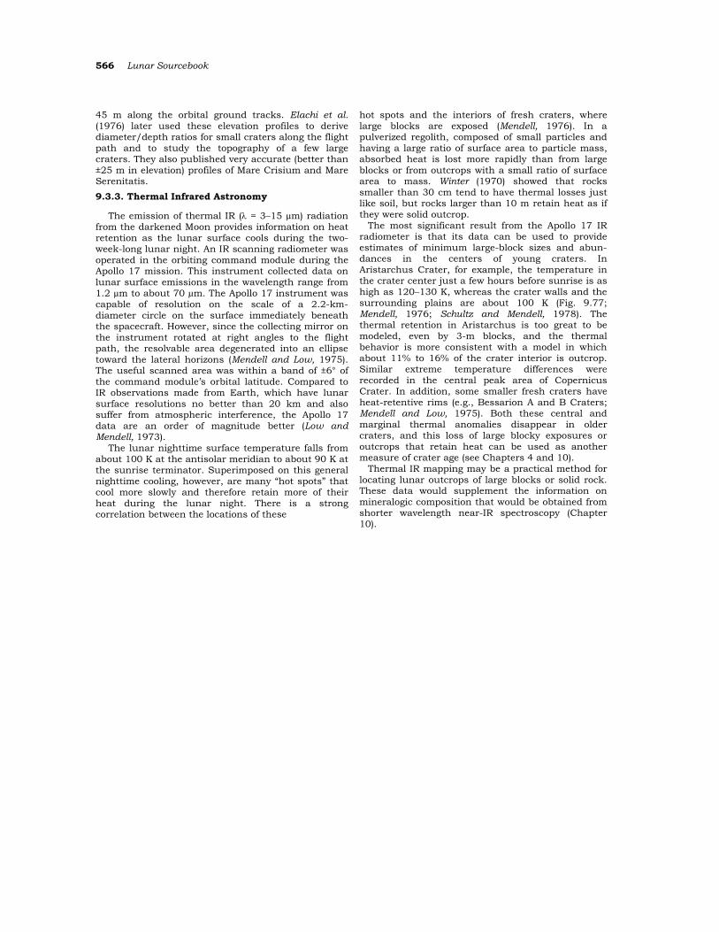
566 Lunar Sourcebook
45 m along the orbital ground tracks. Elachi et al. (1976) later used these elevation profiles to derive diameter/depth ratios for small craters along the flight path and to study the topography of a few large craters. They also published very accurate (better than ±25 m in elevation) profiles of Mare Crisium and Mare Serenitatis. 9.3.3. Thermal Infrared Astronomy
The emission of thermal IR (λ = 3–15 µm) radiation from the darkened Moon provides information on heat retention as the lunar surface cools during the two-week-long lunar night. An IR scanning radiometer was operated in the orbiting command module during the Apollo 17 mission. This instrument collected data on lunar surface emissions in the wavelength range from 1.2 µm to about 70 µm. The Apollo 17 instrument was capable of resolution on the scale of a 2.2-km-diameter circle on the surface immediately beneath the spacecraft. However, since the collecting mirror on the instrument rotated at right angles to the flight path, the resolvable area degenerated into an ellipse toward the lateral horizons (Mendell and Low, 1975). The useful scanned area was within a band of ±6° of the command module’s orbital latitude. Compared to IR observations made from Earth, which have lunar surface resolutions no better than 20 km and also suffer from atmospheric interference, the Apollo 17 data are an order of magnitude better (Low and Mendell, 1973).
The lunar nighttime surface temperature falls from about 100 K at the antisolar meridian to about 90 K at the sunrise terminator. Superimposed on this general nighttime cooling, however, are many “hot spots” that cool more slowly and therefore retain more of their heat during the lunar night. There is a strong correlation between the locations of these
hot spots and the interiors of fresh craters, where large blocks are exposed (Mendell, 1976). In a pulverized regolith, composed of small particles and having a large ratio of surface area to particle mass, absorbed heat is lost more rapidly than from large blocks or from outcrops with a small ratio of surface area to mass. Winter (1970) showed that rocks smaller than 30 cm tend to have thermal losses just like soil, but rocks larger than 10 m retain heat as if they were solid outcrop.
The most significant result from the Apollo 17 IR radiometer is that its data can be used to provide estimates of minimum large-block sizes and abun-dances in the centers of young craters. In Aristarchus Crater, for example, the temperature in the crater center just a few hours before sunrise is as high as 120–130 K, whereas the crater walls and the surrounding plains are about 100 K (Fig. 9.77; Mendell, 1976; Schultz and Mendell, 1978). The thermal retention in Aristarchus is too great to be modeled, even by 3-m blocks, and the thermal behavior is more consistent with a model in which about 11% to 16% of the crater interior is outcrop. Similar extreme temperature differences were recorded in the central peak area of Copernicus Crater. In addition, some smaller fresh craters have heat-retentive rims (e.g., Bessarion A and B Craters; Mendell and Low, 1975). Both these central and marginal thermal anomalies disappear in older craters, and this loss of large blocky exposures or outcrops that retain heat can be used as another measure of crater age (see Chapters 4 and 10).
Thermal IR mapping may be a practical method for locating lunar outcrops of large blocks or solid rock. These data would supplement the information on mineralogic composition that would be obtained from shorter wavelength near-IR spectroscopy (Chapter 10).
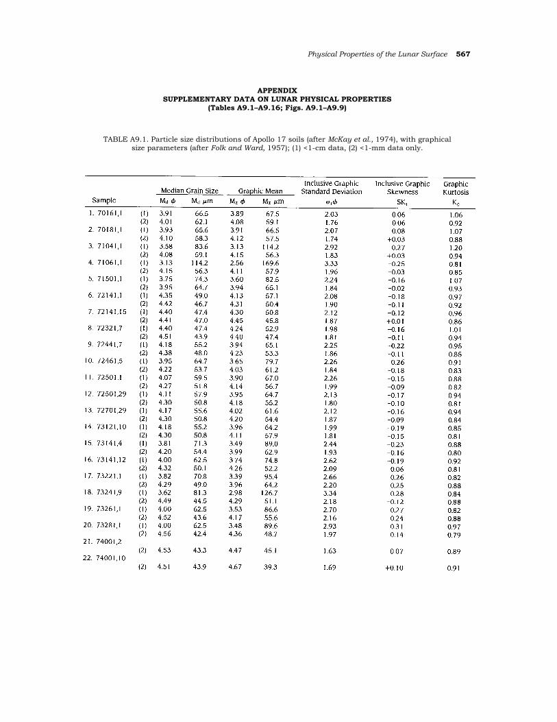
Physίcal Propertίes of the Lunar Surface 567
APPENDIX SUPPLEMENTARY DATA ΟΝ LUNAR PHYSICAL PROPERTIES
(Tables Α9.1–Α9.16; Figs. Α9.1–Α9.9)
TABLE A9.1. Particle size distributions of Apollo 17 soils (after McKay et al., 1974), with graphical size parameters (after Folk and Ward, 1957); (1) <1-cm data, (2) <1-mm data only.
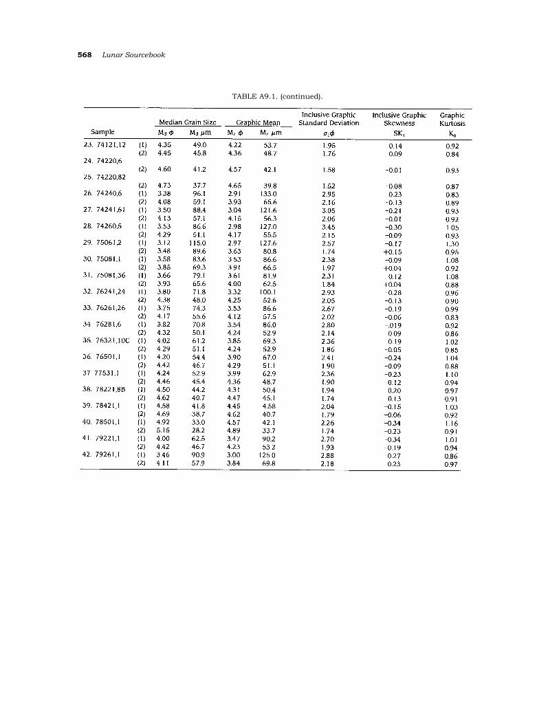
568 Lunar Sourcebook
TABLE Α9.1. (continued).
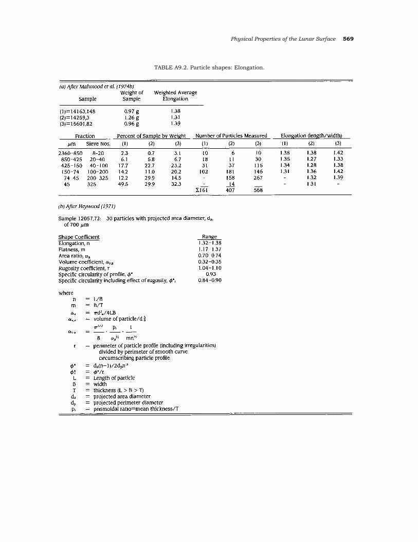
Physical Properties of the Lunar Surface 569
TABLE Α9.2. Particle shapes: Elongation.
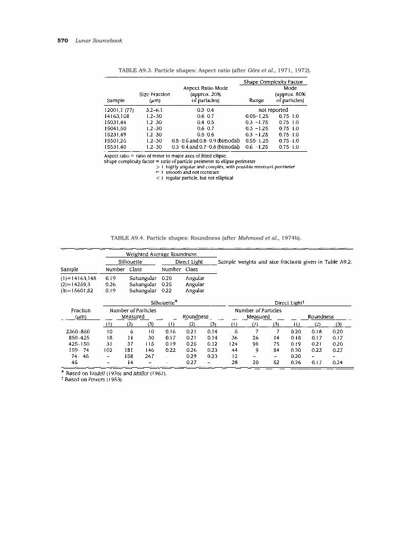
570 Lunar Sourcebook
TABLE Α9.3. Particle shapes: Aspect ratio (after Görz et al., 1971, 1972).
TABLE Α9.4. Particle shapes: Roundness (after Mahmood et al., 1974b).
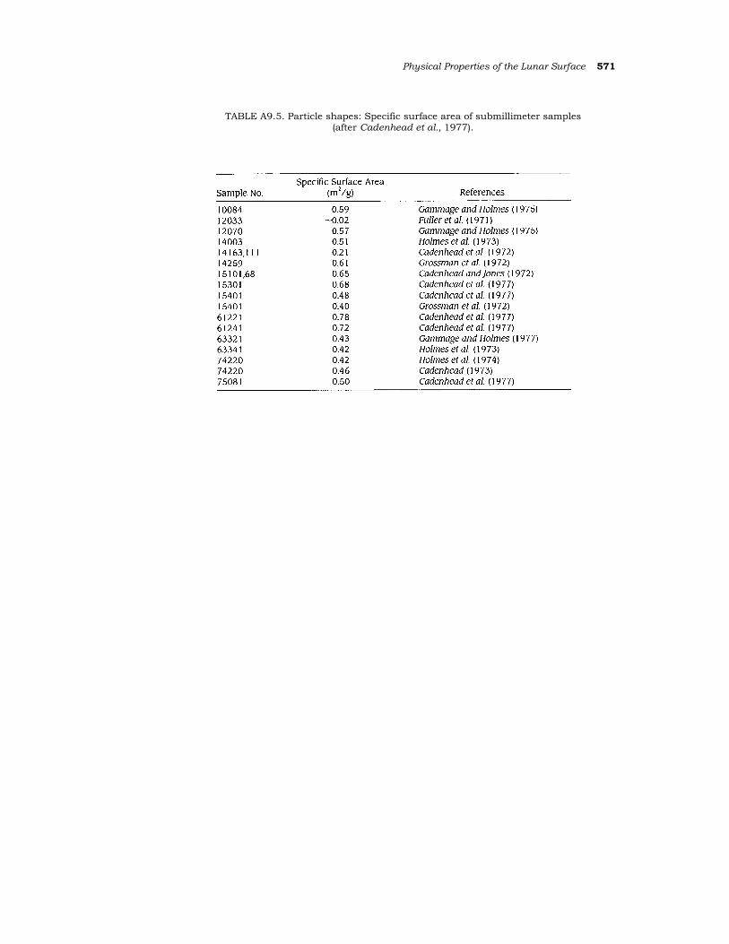
Physical Properties of the Lunar Surface 571
TABLE Α9.5. Particle shapes: Specific surface area of submillimeter samples (after Cadenhead et al., 1977).
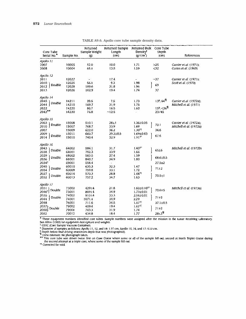
572 Lunar Sourcebook
TABLE Α9.6. Apollo core tube sample density data.
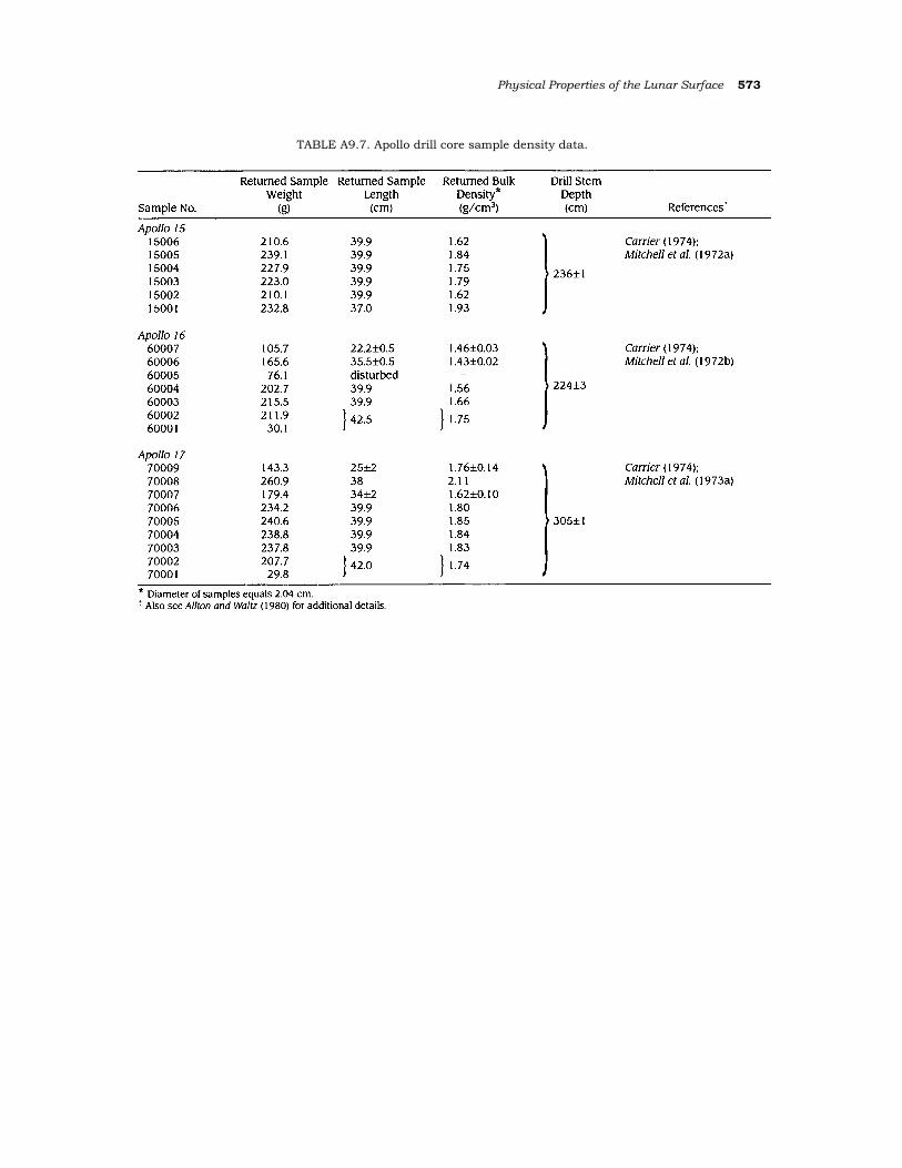
Physical Properties of the Lunar Surface 573
TABLE Α9.7. Apollo drill core sample density data.
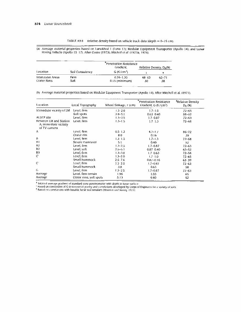
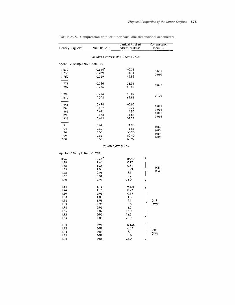
Physical Properties of the Lunar Surface 575
TABLE A9.9. Compression data for lunar soils (one-dimensional oedometer).
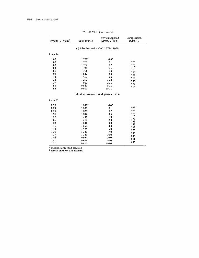
576 Lunar Sourcebook
TABLE Α9.9. (continued).
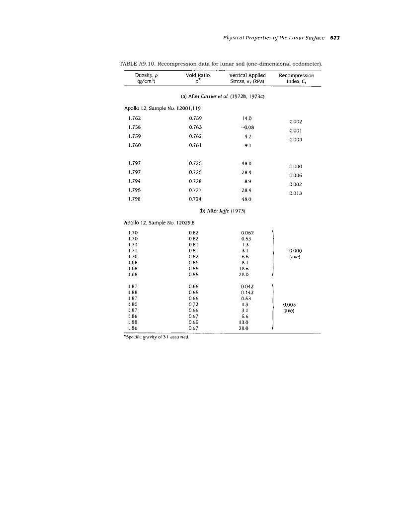
TABLE Α9.10. Recompression data for lunar soil (one-dimensional oedometer).
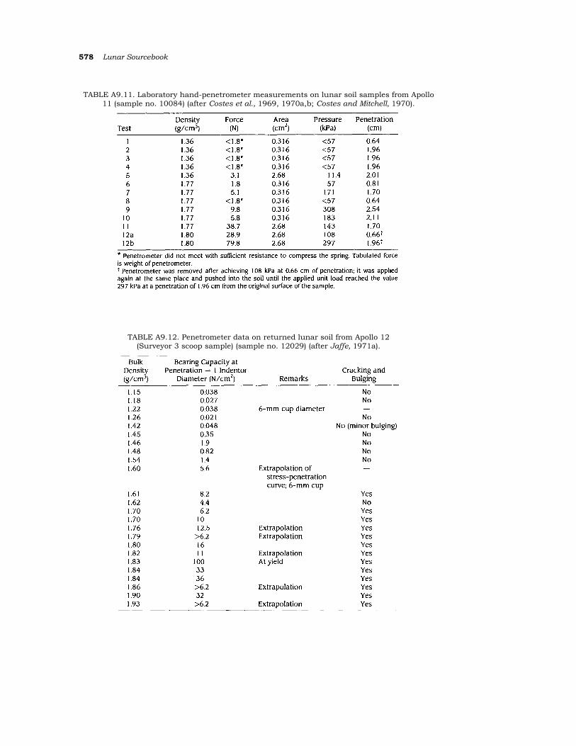
578 Lunar Sourcebook
TABLE Α9.11. Laboratory hand-penetrometer measurements on lunar soil samples from Apollo 11 (sample no. 10084) (after Costes et al., 1969, 1970a,b; Costes and Mitchell, 1970).
TABLE Α9.12. Penetrometer data on returned lunar soil from Apollo 12 (Surveyor 3 scoop sample) (sample no. 12029) (after Jaffe, 1971a).
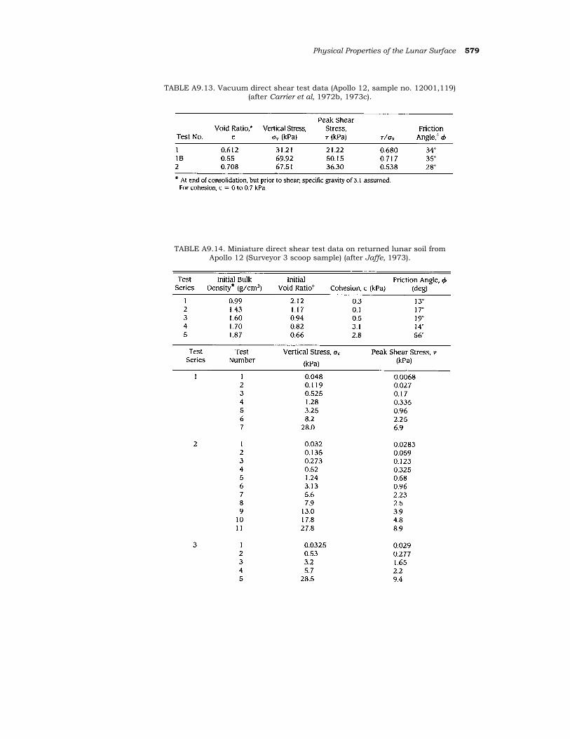
Physical Properties of the Lunar Surface 579
TABLE A9.13. Vacuum direct shear test data (Apollo 12, sample no. 12001,119) (after Carrier et al, 1972b, 1973c).
TABLE A9.14. Miniature direct shear test data on returned lunar soil from Apollo 12 (Surveyor 3 scoop sample) (after Jaffe, 1973).
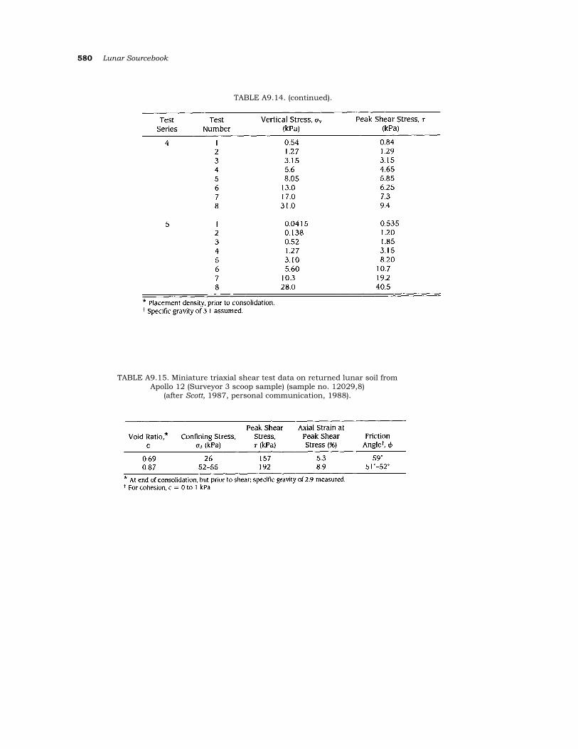
580 Lunar Sourcebook
TABLE Α9.14. (continued).
TABLE Α9.15. Miniature triaxial shear test data on returned lunar soil from Apollo 12 (Surveyor 3 scoop sample) (sample no. 12029,8)
(after Scott, 1987, personal communication, 1988).
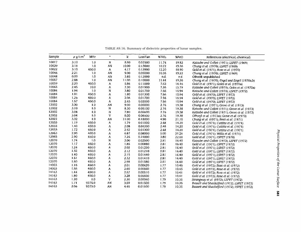
TABLE Α9.16. Summary of dielectric properties of lunar samples.
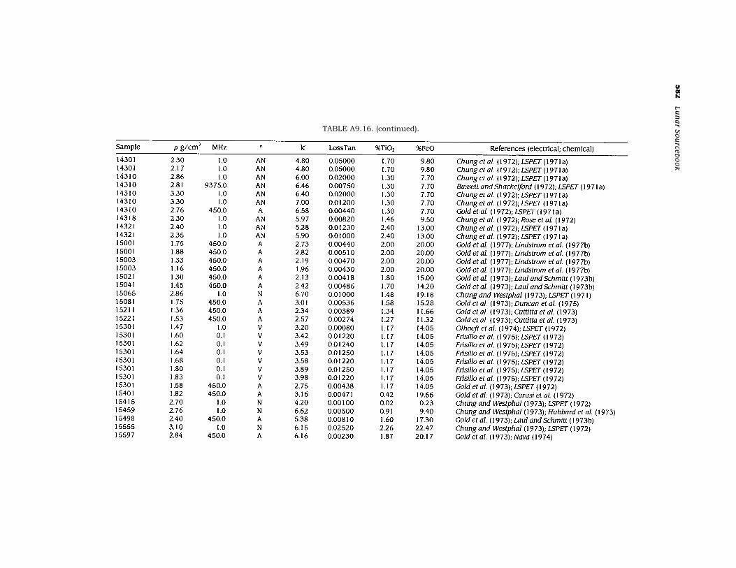
TABLE Α9.16. (continued).
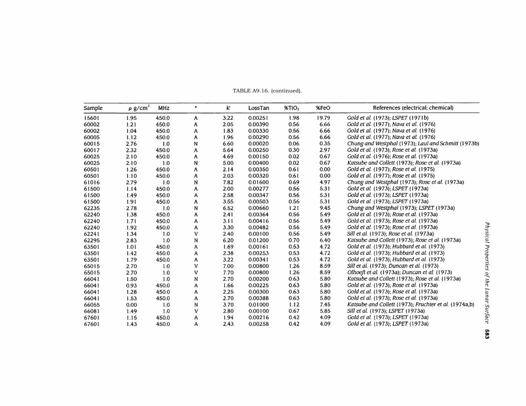
TABLE Α9.16. (continued).
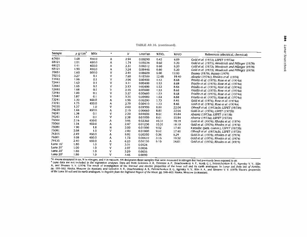
TABLE Α9.16. (continued).
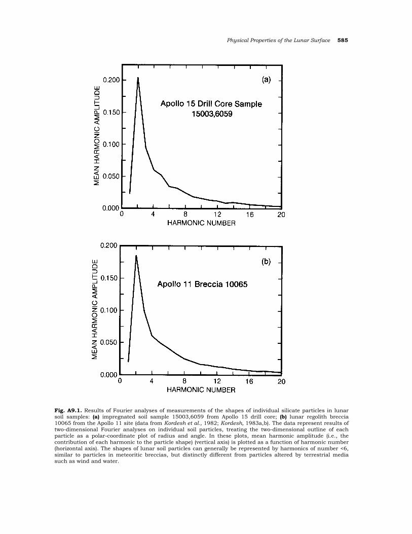
Physical Properties of the Lunar Surface 585
Fig. A9.1. Results of Fourier analyses of measurements of the shapes of individual silicate particles in lunar soil samples: (a) impregnated soil sample 15003,6059 from Apollo 15 drill core; (b) lunar regolith breccia 10065 from the Apollo 11 site (data from Kordesh et al., 1982; Kordesh, 1983a,b). The data represent results of two-dimensional Fourier analyses on individual soil particles, treating the two-dimensίonal outline of each particle as a polar-coordinate plot of radius and angle. In these plots, mean harmonic amplitude (i.e., the contributίon of each harmonic to the particle shape) (vertical axis) is plotted as a function of harmonίc number (horizontal axis). The shapes of lunar soil particles can generally be represented by harmonics of number <6, similar to particles in meteoritic breccias, but distinctly different from partίcles altered by terrestrial media such as wind and water.
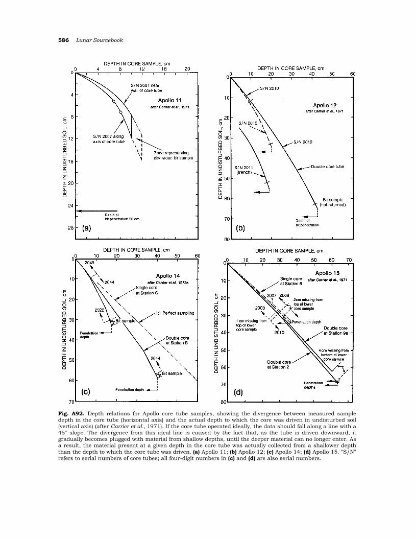
586 Lunar Sourcebook
Fig. Α92. Depth relatίons for Apollo core tube samples, showing the divergence between measured sample depth in the core tube (horizontal axis) and the actual depth to which the core was driven in undisturbed soil (vertical axis) (after Carrier et al., 1971). If the core tube operated ideally, the data should fall along a line with a 45° slope. The divergence from this ideal line is caused by the fact that, as the tube is driven downward, it gradually becomes plugged with material from shallow depths, until the deeper material can no longer enter. As a result, the material present at a given depth in the core tube was actually collected from a shallower depth than the depth to which the core tube was driven. (a) Apollo 11; (b) Apollo 12; (c) Apollo 14; (d) Apollo 15. “S/N” refers to serial numbers of core tubes; all four-digit numbers in (c) and (d) are also serial numbers.
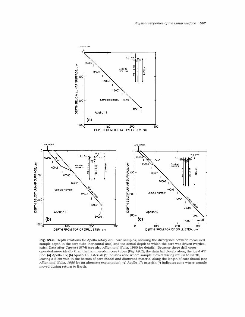
Physical Properties of the Lunar Surface 587
Fig. A9.3. Depth relations for Apollo rotary drill core samples, showing the divergence between measured sample depth in the core tube (horizontal axis) and the actual depth to which the core was driven (vertical axis). Data after Carrier (1974) (see also Allton and Waltz, 1980 for details). Because these drill cores operated more ideally than the hammered-in core tubes (Fig. A9.2), the data fall closely along the ideal 45° line. (a) Apollo 15; (b) Apollo 16: asterisk (*) indiates zone where sample moved during return to Earth, leaving a 5-cm void in the bottom of core 60006 and disturbed material along the length of core 60005 (see Allton and Waltz, 1980 for an alternate explanation); (c) Apollo 17: asterisk (*) indicates zone where sample moved during return to Earth.
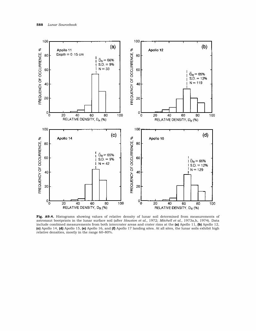
588 Lunar Sourcebook
Fig. Α9.4. Histograms showing values of relative density of lunar soil determined from measurements of astronaut bootprints in the lunar surface soil (after Houston et al., 1972; Mitchell et al., 1973a,h, 1974). Data include combined measurements from both intercrater areas and crater rims at the (a) Apollo 11, (b) Apollo 12, (c) Apollo 14, (d) Apollo 15, (e) Apollo 16, and (f) Apollo 17 landing sites. At all sites, the lunar soils exhibit high relative densities, mostly in the range 60–80%.
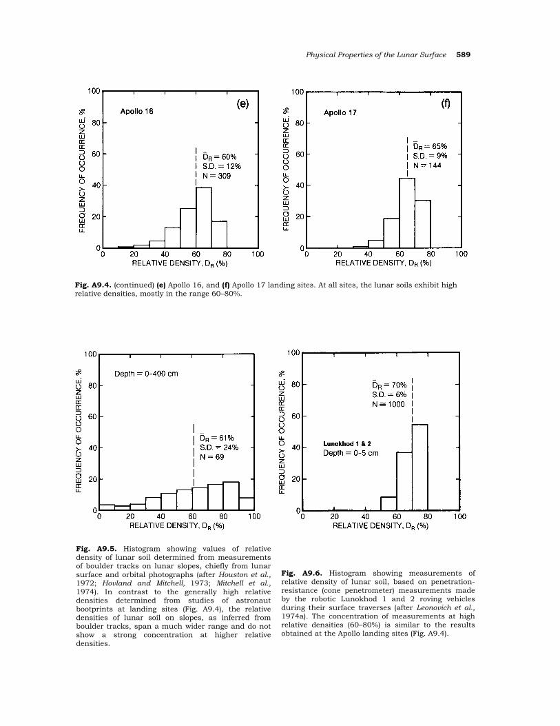
Physical Properties of the Lunar Surface 589
Fig. Α9.4. (continued) (e) Apollo 16, and (f) Apollo 17 landing sites. At all sites, the lunar soils exhibit high relative densities, mostly in the range 60–80%.
Fig. Α9.5. Histogram showing values of relative density of lunar soil determined from measurements of boulder tracks on lunar slopes, chiefly from lunar surface and orbital photographs (after Houston et al., 1972; Hovland and Mitchell, 1973; Mitchell et al., 1974). In contrast to the generally high relative densities determined from studies of astronaut bootprints at landing sites (Fig. Α9.4), the relative densities of lunar soil on slopes, as inferred from boulder tracks, span a much wider range and do not show a strong concentration at higher relative densities.
Fig. Α9.6. Histogram showing measurements of relative density of lunar soil, based on penetration-resistance (cone penetrometer) measurements made by the robotic Lunokhod 1 and 2 roving vehicles during their surface traverses (after Leonovich et al., 1974a). The concentration of measurements at high relative densities (60–80%) is similar to the results obtained at the Apollo landing sites (Fig. Α9.4).
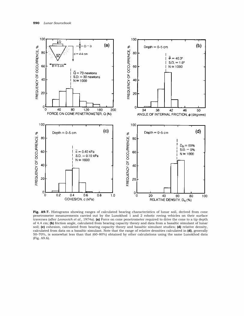
590 Lunar Sourcebook
Fig. Α9.7. Histograms showing ranges of calculated bearing characteristics of lunar soil, derived from cone penetrometer measurements carried out by the Lunokhod 1 and 2 robotic roving vehicles on their surface traverses (after Leonovich et al., 1974a). (a) Force on cone penetrometer required to drive the cone to a tip depth of 4.4 cm; (b) friction angle, calculated from bearing capacίty theory and data from a basaltic sίmulant of lunar soil; (c) cohesion, calculated from bearing capacity theory and basaltic simulant studies; (d) relative density, calculated from data on a basaltic simulant. Note that the range of relative densities calculated in (d), generally 50–70%, is somewhat less than that (60–80%) obtained by other calculations using the same Lunokhod data (Fig. Α9.6).
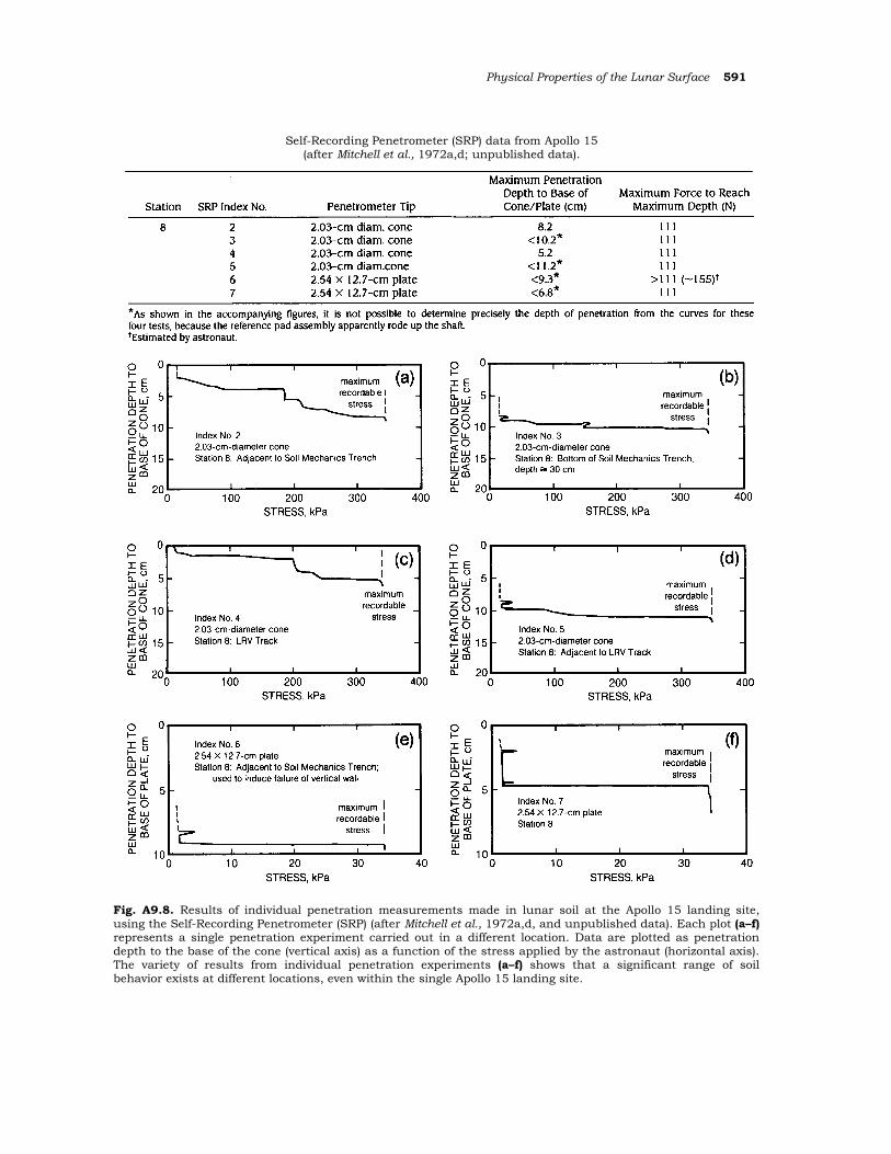
Physical Properties of the Lunar Surface 591
Self-Recordίng Penetrometer (SRP) data from Apollo 15 (after Mitchell et al., 1972a,d; unpublished data).
Fig. Α9.8. Results of individual penetration measurements made in lunar soil at the Apollo 15 landing site, using the Self-Recording Penetrometer (SRP) (after Mitchell et al., 1972a,d, and unpublished data). Each plot (a–f) represents a single penetration experiment carried out ίn a different location. Data are plotted as penetration depth to the base of the cone (vertical axis) as a function of the stress applied by the astronaut (horizontal axis). The variety of results from individual penetration experiments (a–f) shows that a significant range of soil behavior exίsts at different locations, even within the single Apollo 15 landing site.
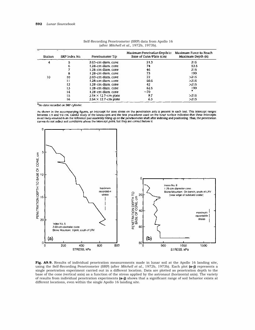
592 Lunar Sourcebook
Self-Recording Penetrometer (SRP) data from Apollo 16 (after Mitchell et al., 1972b, 1973b).
Fig. Α9.9. Results of individual penetration measurements made in lunar soil at the Apollo 16 landing site, using the Self-Recording Penetrometer (SRP) (after Mitchell et al., 1972b, 1973b). Each plot (a–j) represents a single penetration experiment carried out in a different location. Data are plotted as penetration depth to the base of the cone (vertical axis) as a function of the stress applied by the astronaut (horizontal axis). The variety of results from individual penetration experiments (a–j) shows that a significant range of soil behavior exists at different locations, even within the single Apollo 16 landing site.
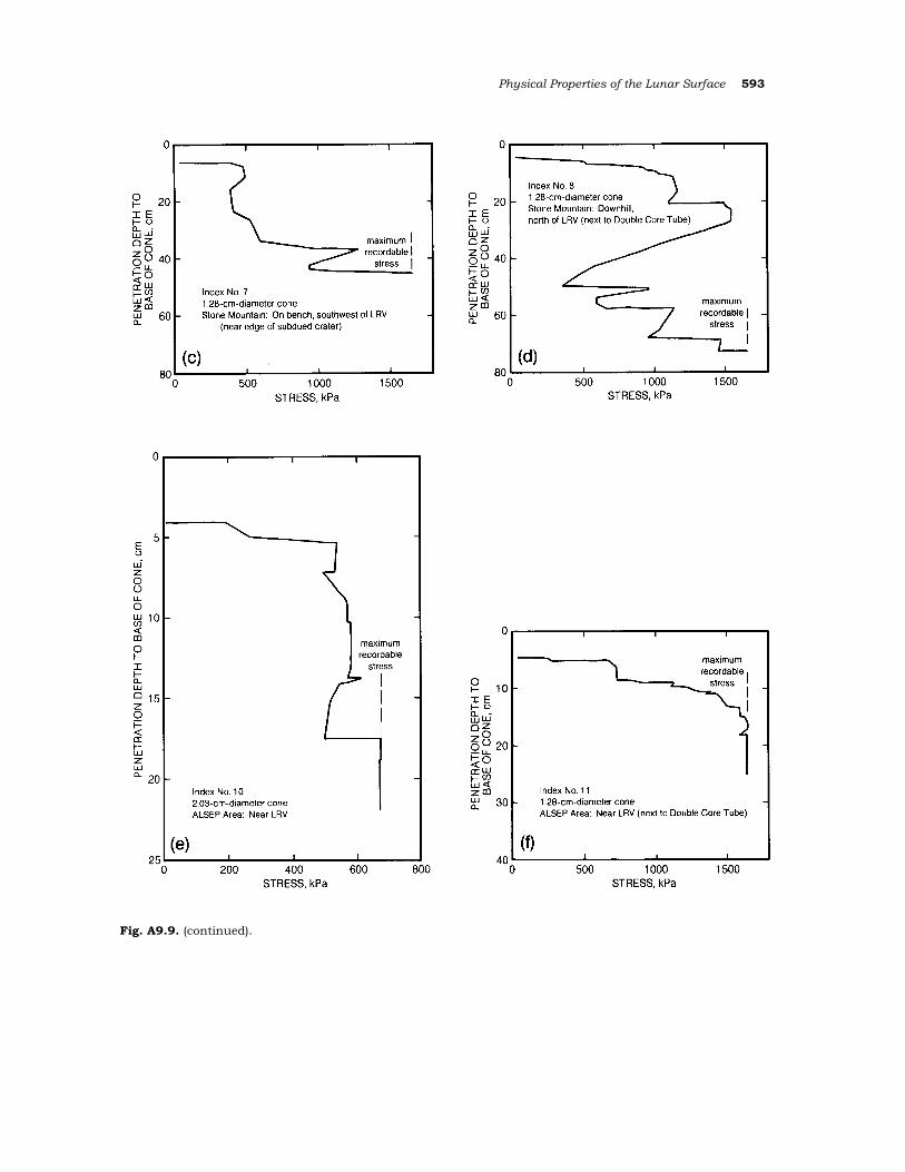
Physical Properties of the Lunar Surface 593
Fig. Α9.9. (continued).
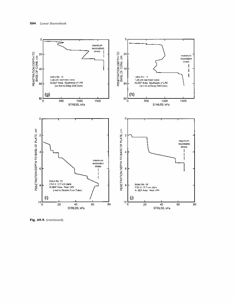
594 Lunar Sourcebook
Fig. Α9.9. (continued).


![⃝[anthony young] lunar and planetary rovers](https://img.pdfslide.net/doc/110x75/568caa611a28ab186da15ce8/anthony-young-lunar-and-planetary-rovers.jpg)