Embed Size (px)
Citation preview
Physically Based Mountain Hydrological Modeling Using ReanalysisData in Patagonia
SEBASTIAN A. KROGH
Department of Civil Engineering, Universidad de Chile, Santiago, Chile
JOHN W. POMEROY
Centre for Hydrology, University of Saskatchewan, Saskatoon, Saskatchewan, Canada
JAMES MCPHEE
Department of Civil Engineering, and Advanced Mining Technology Center, Universidad
de Chile, Santiago, Chile
(Manuscript received 30 October 2013, in final form 15 August 2014)
ABSTRACT
A physically based hydrological model for the upper Baker River basin (UBRB) in Patagonia was de-
veloped using the modular Cold Regions Hydrological Model (CRHM) in order to better understand the
processes that drive the hydrological response of one of the largest rivers in this region. The model includes
a full suite of blowing snow, intercepted snow, and energy balance snowmelt modules that can be used to
describe the hydrology of this cold region. Within this watershed, snowfall, wind speed, and radiation are not
measured; there are no high-elevation weather stations; and existing weather stations are sparsely distributed.
The impact of atmospheric data fromECMWF interim reanalysis (ERA-Interim) andClimate Forecast System
Reanalysis (CFSR) on improving model performance by enhancing the representation of forcing variables was
evaluated. CRHM parameters were assigned for local physiographic and vegetation characteristics based on
satellite land cover classification, a digital elevation model, and parameter transfer from cold region environ-
ments in western Canada. It was found that observed precipitation has almost no predictive power [Nash–
Sutcliffe coefficient (NS), 0.3]when used to force the hydrologicmodel, whereasmodel performanceusing any
of the reanalysis products—after bias correction—was acceptable with very little calibration (NS . 0.7). The
modeled water balance shows that snowfall amounts to about 28% of the total precipitation and that 26% of
total river flow stems from snowmelt. Evapotranspiration losses account for 7.2%of total precipitation, whereas
sublimation and canopy interception losses represent about 1%. The soil component is the dominantmodulator
of runoff, with infiltration contributing as much as 73.7% to total basin outflow.
1. Introduction
Chilean Patagonia contains some of the largest water
reserves in the southern cone of South America. Tied
with economic growth, increasing energy demands have
turned public attention to the region’s rivers (the largest
in Chile) and their yet untapped hydropower potential.
Although the statistical properties of flow for the major
rivers in the area are known because of a reasonably
comprehensive hydrometric network, the processes re-
sponsible for the hydrology of Patagonia are poorly
understood, and so the reliability of historical information
for streamflow prediction cannot be evaluated. In light of
ongoing environmental change, hydrological investiga-
tions are crucial to achieve a better understanding of en-
vironmental systems dynamics and their possible response
to human interference across spatial and temporal scales.
A particular concern is climate change, which has recently
resulted in substantial glacier retreat in the region (Rivera
et al. 2007) with unknown impacts on river flow.
In spite of these concerns, very few studies of the hy-
drology and climatology of the region have been con-
ducted. Aravena (2007) developed a 400-yr precipitation
Corresponding author address: James McPhee, Department of
Civil Engineering, Universidad de Chile, Av. Blanco Encalada
2002, Santiago 8370449, Chile.
E-mail: [email protected]
172 JOURNAL OF HYDROMETEOROLOGY VOLUME 16
DOI: 10.1175/JHM-D-13-0178.1
� 2015 American Meteorological Society
reconstruction using tree ring data and glacier fluctua-
tions in the Austral Chilean Andes, finding important
decadal variations for the northwest and central Patago-
nia and also a strong biannual oscillation for the south-
ernmost region. Garreaud et al. (2009) described the
mean annual and decadal patterns of precipitation in
South America and how they are influenced both by cli-
matic indexes (Pacific decadal oscillation, Antarctic
Oscillation, and El Niño–Southern Oscillation) and oro-
graphic effects using a large-scale paleoclimatic approach.
Lopez et al. (2008) studied variability in snow-covered
areas (SCAs) of the Northern Patagonian Ice Field
(NPIF) during 2000–06 and correlated SCA to precip-
itation and air temperature, obtaining the highest corre-
lations for temperature (r2 5 0.75). Rivera et al. (2007)
quantified decreases in the NPIF of up to 4.0 60.97myr21 for ice thickness and up to 3.2% 6 1.5% or
140 6 61km2 for area over 1975–2001, based on remote
sensing and in situ data.
Although the above studies represent improvements
on their respective fields, there remains a major gap in
published comprehensive hydrological investigations in
the region. Dussaillant et al. (2012) present the first
description of the main hydrological patterns (pre-
cipitation, temperature, and streamflow) of the Baker
River basin using observed data. They also discuss the
difficulties associated with undertaking this task given
the sparse distribution of gauging stations, together with
the significant topographical and climatological gradi-
ents existing in the region. Barría (2010) developed
a statistical approach for obtaining monthly streamflow
forecasts for the Baker and Pascua river basins. How-
ever, because this research was entirely data driven, it
does not increase knowledge of the physical processes
governing water movements in the basin. Given the
combination of climate change and increased pressure
to use the water resources in the region, it becomes
paramount for the scientific and decision-making
community to increase their knowledge on the hy-
drological functioning of this relatively pristine envi-
ronmental system.
Physically based models offer the opportunity of
comprehending physical interactions between processes
and variables within the hydrological cycle, an advan-
tage that cannot be achieved with other types of models
(empirical, conceptual, or statistical, for example). The
Cold Regions Hydrological Model (CRHM; Pomeroy
et al. 2007) is a physically based model developed at the
Centre for Hydrology, University of Saskatchewan, with
the aim of improving the understanding of hydrological
processes in cold environments, which are particular in
the sense that a host of specific phenomena such as snow
and ice accumulation, interception, transport and melt,
infiltration through frozen soils, and cold water bodies
control the hydrograph timing. CRHM has a limited
need for calibration (Pomeroy et al. 2007), and most
(but not all) of its parameters can be inferred from in-
tensive field or modeling studies. This, together with its
modular nature and open structure, makes it particularly
suitable for testing hydrological hypothesis in poorly
gauged or ungauged basins. Gonthier (2011) developed
the first hydrological study in Chile using CRHM. He
analyzed three high mountain basins in the Chilean
semiaridAndes (328S), calibrating parameters regarding
soil moisture and routing processes against streamflow
records. All results showed Nash–Sutcliffe coefficient
(NS) values below 0.6 and overestimation of snow ac-
cumulation up to 400%with respect to local snow pillow
data. Poor modeling results were attributed in part to
the very low density of meteorological measurements
within the basin and thus great uncertainty in meteo-
rological driving variables. Fang and Pomeroy (2007)
developed a CRHM with the aim of understanding the
dynamical processes that govern drought phenomena in
the Canadian prairies. A sensitivity analysis to meteo-
rological input data was carried out, showing that even
under moderate drought scenarios of 15% reduction in
winter precipitation and 2.58C increase in winter mean
air temperature, spring runoff may disappear com-
pletely. Ellis et al. (2010) developed a CRHM to assess
the differences in snowmelt and snow accumulation in
forest and clearing sites, achieving an NS model effi-
ciency value of 0.51 for snow water equivalent (SWE),
with slightly better representation on clearing sites;
these results show the CRHM predictive potential when
no calibration is undertaken. Another study was de-
veloped by Fang and Pomeroy (2009), who character-
ized blowing snow redistribution in prairie wetlands,
obtaining good results either with an aggregated or
a fully distributed spatial representation. Pomeroy et al.
(2012) developed a CRHM in a forested mountainous
basin with minimal calibration in order to simulate the
impacts of forest disturbance in the basin hydrology.
Results show different streamflow volume responses
for each scenario, ranging from 2% for small forest
reduction impacts to 8% for a complete forest-burning
event. A recent study developed a CRHM for an alpine
to subalpine Canadian Rockies catchment and evalu-
ated uncalibrated model performance against snow
accumulation, soil moisture, groundwater, and sub-
basin and basin streamflow over several years (Fang
et al. 2013) with acceptable predictive performance for
all variables except groundwater. Tests of CRHM in
alpine and steppe environments of the Qinghai Tibetan
Plateau show good performance for snowpack, runoff,
and streamflow simulation when blowing snow, energy
FEBRUARY 2015 KROGH ET AL . 173
balance snowmelt, and frozen soil infiltration options
are used (Zhou et al. 2014).
Atmospheric reanalyses are a scientific method for
developing a comprehensive record of weather and cli-
mate change over time and can complement the infor-
mation provided by scarce meteorological observations in
remote regions in order to obtain surface meteorology to
force land surface models (Sheffield et al. 2004). Quoting
Saha et al. (2010, p. 1015), ‘‘[t]he general purpose of
conducting reanalyses is to produce multiyear global
state-of-the-art gridded representations of atmospheric
states, generated by a constant model and a constant
data assimilation system.’’ The current generation of
reanalyses assimilates data from satellite observations;
in situ surface measurements such as 2-m temperature,
relative humidity, and wind speed; and upper-atmosphere
variables from radiosondes, wind profilers, and aircraft
(Dee et al. 2011; Saha et al. 2010). In this study, we test two
of themost recent products available: theNationalCenters
for Environmental Prediction–National Center for At-
mospheric Research (NCEP–NCAR) Climate Forecast
System Reanalysis (CFSR) and the European Centre
forMedium-RangeWeather Forecasts (ECMWF) interim
reanalysis (ERA-Interim). ERA-Interim is the latest
global atmospheric reanalysis produced by the ECMWF,
and it covers the period from 1 January 1989 to the
present. The gridded data product includes a large
variety of 3-hourly surface parameters and 6-hourly
upper-air parameters (Dee et al. 2011). This reanalysis
has a spatial resolution of 1.58 and 37 pressure levels
[increasing by 14 levels from the preceding version
40-yr ECMWF Re-Analysis (ERA-40)]. On the other
hand, CFSR spans the 31-yr period from 1979 to 2009. It
was designed to be a high-resolution coupled atmosphere–
ocean–land surface–sea ice system and to provide the
best estimation of the state of these domains over this
period (Saha et al. 2010). Its spatial resolution varies
from 0.258 at the equator to 0.58 beyond the tropics,
with 40 pressure levels. Ward et al. (2011) evaluate
several precipitation products [ERA-40, NCEP–
NCAR Global Reanalysis 1 (R-1), Precipitation Esti-
mation from Remotely Sensed Imagery Using Artificial
Neural Networks (PERSIANN), and Tropical Rainfall
Measuring Mission (TRMM)] over the Andes Cordil-
lera (Baker and Paute basins, Chile–Argentina and
Ecuador, respectively), comparing them with observed
data interpolations based on Thiessen polygons. For the
Baker River basin, precipitation products were always
above observed data, which can be explained by the low
density and low elevation of the station. Ward et al.
(2011) also highlighted the secondary importance of the
interpolation scheme used, arguing that errors in in-
terpolation are dominated by the low density of rain
gauges throughout the Baker basin. Silva et al. (2011)
compared CFSR and other NCEP–NCAR reanalyses,
that is, R-1 and the NCEP–U.S. Department of Energy
(DOE) Second Atmospheric Model Intercomparison
Project (AMIP-II; R-2), over South America. Over the
Andes Cordillera, in particular, all three reanalyses
(CFSR, R-1, and R-2) seem to overestimate total pre-
cipitation, but significant improvements are associated
with CFSR, probably because of its higher spatial reso-
lution and better representation of regional topography.
The objective of this paper is to describe the first in-
depth analysis of the hydrological function of the upper
Baker River basin (UBRB), based on a physically based
hydrological model (CRHM) driven using meteorolog-
ical station observations and global meteorological
model reanalyses. Hence, the main goals of this research
are (i) to describe a plausible combination of hydro-
logical processes giving rise to the observed streamflow
record in order to enable future global change impact
assessments and (ii) to demonstrate the value of
reanalysis data in combination with a physically based
hydrologic model in achieving the former goal. In this
paper, we also highlight the existing information gaps
that preclude a better understanding of the hydrology
of the region and suggest future avenues for improving
such knowledge.
2. Study site and observations
a. Location
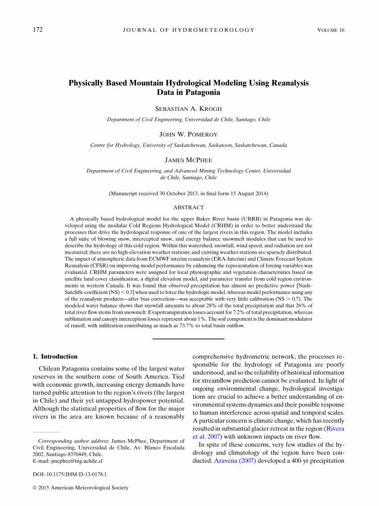
TheUBRB is defined by the Bertrand Lake outlet and
has an area of 15 904 km2 (see Fig. 1). At this location,
the Baker River has a mean annual discharge of
566m3 s21 (Fig. 3), being the largest river in Chile when
it reaches the ocean. The basin is characterized by very
heterogeneous climate, geology, and land cover fea-
tures, with landscape types that include glaciers and
icefields [2787 km2 (17.5%)], rivers and lakes [2109 km2
(13.3%)], dense forest [2777 km2 (17.5%)], grassland
and shrubland [5984 km2 (37.6%)], peatlands [66 km2
(0.4%)], and bare rock [2181 km2 (13.7%)] (CONAF/
CONAMA 1999; see Fig. 7, described in greater detail
below). The regional climate is dominated by the in-
teraction of weather fronts traveling east from the Pa-
cific Ocean with the topographic barrier of the Andes
Cordillera. Here, mountains reach from 200 up to
4000m MSL over a distance of less than 100 km and
generate a steep west-to-east precipitation gradient
(Warren and Sugden 1993); as a result, precipitation in
the mountainous western part of the basin can reach
more than 2000mm annually, whereas the low-lying
eastern region has a steppe-like climate (Pampas) with
annual precipitation on the order of 400mm(seeFigs. 2, 4).
174 JOURNAL OF HYDROMETEOROLOGY VOLUME 16
Although precipitation decreases somewhat during the
spring–summer season (September–March), rainy con-
ditions persist throughout the year. Air temperature
reaches freezing conditions during the winter (June–
August) season, whereas maximum summer tempera-
tures usually oscillate around 158C. The prevalence of
cold conditions indicates that snow and ice formation and
melt should be a dominating process in the region’s
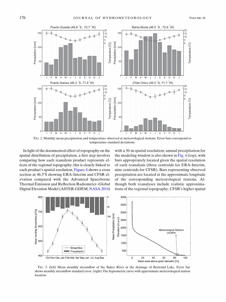
hydrology. Figure 3 illustrates this effect, with UBRB
flows peaking during the warm season (February) with
a strong seasonal pattern.
b. Observed data
Standard streamflow and meteorological data are
available from stations operated by the DirecciónGeneral de Aguas (National Water Directorate) ofChile. Streamflow is more reliably measured than pre-cipitation in the region, mainly because only rainfall butnot snowfall is measured and because of the sparsenessof the rainfall gauge network and gaps in the rainfall datarecords. Rainfall observations are only available in val-ley bottom locations, with no measurements in themountains where most runoff occurs. Rainfall that ismeasured is subject to undercatch because of wind andfreezing effects, whereas streamflow measurements areobtained in mostly stable river sections with rating
curves that are updated periodically (B. Nazarala,Dirección General de Aguas, 2014, personal communi-cation). Tables 1 and 2 show information on the existing
stations. Data gaps in weather stations, sometimes rep-
resenting up to 83% of a station’s records within
a modeling period, prevented the use of all station re-
cords existing for the region. The density of rain gauge
stations over the basin is approximately 0.2 stations per
1000 km2. This value is compared with the recommen-
dation of the World Meteorological Organization
(WMO 1994), which set a minimum precipitation station
density of 1 station per 250km2 or 4 stations per 1000 km2
for mountainous regions; this suggests that UBRB in-
strumentation is below international standards.
c. Reanalysis of precipitation
Atmospheric model data from ERA-Interim and
CFSR were considered in an attempt to overcome the
lack of snowfall measurements and the limited number
and unrepresentative location of meteorological stations
for hydrological modeling. These data products represent
state-of-the-art global climate characterization and con-
stitute improvements with respect to previous versions.
As a first step for using these as input to the hydrological
model, they are analyzed in the context of local weather
and streamflow data.
FIG. 1. Baker River basin at the drainage of Bertrand Lake. Dashed line shows a cross section at 46.58S.
FEBRUARY 2015 KROGH ET AL . 175
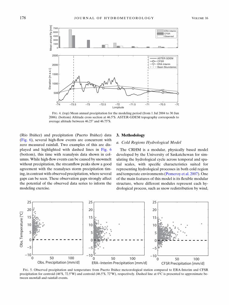
In light of the documented effect of topography on the
spatial distribution of precipitation, a first step involves
comparing how each reanalysis product represents ef-
fects of the regional topography; this is closely linked to
each product’s spatial resolution. Figure 4 shows a cross
section at 46.58S showing ERA-Interim and CFSR el-
evation compared with the Advanced Spaceborne
Thermal Emission and Reflection Radiometer–Global
Digital ElevationModel (ASTER-GDEM; NASA 2014)
with a 30-m spatial resolution; annual precipitation for
the modeling window is also shown in Fig. 4 (top), with
bars appropriately located given the spatial resolution
of each reanalysis (three centroids for ERA-Interim,
nine centroids for CFSR). Bars representing observed
precipitation are located at the approximate longitude
of the corresponding meteorological stations. Al-
though both reanalyses include realistic approxima-
tions of the regional topography, CFSR’s higher spatial
FIG. 2. Monthly mean precipitation and temperature observed at meteorological stations. Error bars correspond to
temperature standard deviations.
FIG. 3. (left) Mean monthly streamflow of the Baker River at the drainage of Bertrand Lake. Error bar
shows monthly streamflow standard error. (right) The hypsometric curve with approximate meteorological station
location.
176 JOURNAL OF HYDROMETEOROLOGY VOLUME 16
resolution allows for a better representation than ERA-
Interim, with steeper and higher topography at the
western side of the basin. Although the absence of ob-
servations renders it impossible to assess which reanalysis
achieves better precipitation estimates at the western
edge of the region, for the central section—around
728W—CFSRmatches the observed values more closely.
When comparing within a reference centroid (728S,46.58W), differences of about 3 times the mean annual
precipitation were detected (682 and 1870mmyr21 for
CFSR and ERA-Interim, respectively). As mentioned
before, CFSR has 3 times the spatial resolution of ERA-
Interim in this region, but in terms of density of centroids
within the basin, the difference rises to 6 times, with six
centroids for CFSR (about 0.4 centroids per 1000km2)
and one centroid for ERA-Interim (0.06 centroids per
1000km2).
A second analysis focused on the meteorological
characteristics of individual storm events as represented
by each data source. This analysis is considered to be
very relevant to runoff generation as the characteristics
of large storms are critical to mountain hydrology re-
gimes. Scatterplots (see Fig. 5) show important differ-
ences; for example, the observed record shows almost no
precipitation events concurrent with air temperatures
below 08C, likely because of the lack of snowfall mea-
surements, whereas reanalysis data show a significant
amount of precipitation occurring at temperatures be-
low 08C, for instance, 127 (17% of all events) and 93
(13% of all events) events for ERA-Interim and CFSR,
respectively, during the modeling period. Given that
snowstorm events are routinely noticed in the region, it
can be concluded that the current precipitation obser-
vational record does not include snowfall, and a low
bias in recorded annual precipitation results from this
lack of measurement. Another difference between re-
analysis and observed data is the fact that most of the
observed precipitation events occur at about 108C,which is 58C above the temperature at which the ma-
jority of precipitation events from the reanalyses occur.
In this context, reanalysis data tend to include colder
precipitation events, with most precipitation occurring
at temperatures below 158C. On the other hand, ob-
served temperatures show precipitation events with
daily temperatures up to 208C; the lack of snowfall
measurements clearly puts a substantial bias on ob-
servations that are expected to have a large impact on
the ability of any mountain hydrology model to simu-
late streamflow.
Also, the total number of precipitation events in the
modeling period differs significantly between reanalysis
and observational data. For example, the weather sta-
tions recorded 216 precipitation events between 1 July
2004 and 30 June 2006, while CFSR and ERA-Interim
produced 664 and 616 events, respectively. Many of
these excess events occurred during the winter season,
which was particularly problematic for weather station
observations. When inspecting observed daily streamflow
TABLE 1. Available weather stations within UBRB.Monthly precipitation and temperature are from within the modeling period (source:
Dirección General de Agua).
Weather station Start End Z (m MSL)
Available monthly
precipitation (%)
Available monthly
temperature (%) SB assignation
Puerto Guadal* Dec 1993 — 210 92 92 SB4, SB5, SB7, SB8
Bahía Murta* Aug 1993 — 240 96 96 SB2, SB7, SB8
Puerto Ibáñez* Dec 1961 — 215 100 96 SB1, SB3, SB6, SB8
Chile Chico Oct 1963 Nov 2004 215 17 0 —
Villa Cerro Castillo Oct 1992 — 345 100 0 —
*Stations used in this study.
TABLE 2. Available stream gauge stations within UBRB.Monthly streamflow is from within modeling period (source: Dirección Generalde Agua).
Stream gauge
station Start End Elev (m MSL)
Mean annual
runoff (m3 s21)
Available monthly
streamflow (%) SB assignation
Río Baker* Apr 1963 — 200 568 100 —
Río Murta* Dec 1985 — 219 93.5 100 SB2
Río Ibáñez* Aug 1970 — 220 158 100 SB1
Río Jeinimeni Dec 1995 Jan 2004 — 27 0.05 —
Río Bagno Dec 1995 — — 1.5 92 —
Río Claro Feb 1985 Nov 2002 — 9.7 0 —
*Stations used in this work.
FEBRUARY 2015 KROGH ET AL . 177
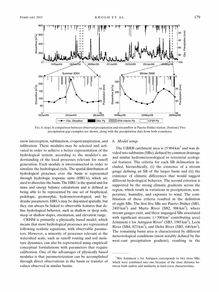
(Río Ibáñez) and precipitation (Puerto Ibáñez) data(Fig. 6), several high-flow events are concurrent with
zero measured rainfall. Two examples of this are dis-
played and highlighted with dashed lines in Fig. 6
(bottom), this time with reanalysis data shown in col-
umns. While high-flow events can be caused by snowmelt
without precipitation, the streamflow peaks show a good
agreement with the reanalyses storm precipitation tim-
ing, in contrast with observed precipitation, where several
gaps can be seen. These observation gaps strongly affect
the potential of the observed data series to inform the
modeling exercise.
3. Methodology
a. Cold Regions Hydrological Model
The CRHM is a modular, physically based model
developed by the University of Saskatchewan for sim-
ulating the hydrological cycle across temporal and spa-
tial scales, with specific characteristics suited for
representing hydrological processes in both cold region
and temperate environments (Pomeroy et al. 2007). One
of the main features of this model is its flexible modular
structure, where different modules represent each hy-
drological process, such as snow redistribution by wind,
FIG. 4. (top) Mean annual precipitation for the modeling period (from 1 Jul 2004 to 30 Jun
2006). (bottom) Altitude cross section at 46.58S. ASTER-GDEM topography corresponds to
average altitude between 46.258 and 46.758S.
FIG. 5. Observed precipitation and temperature from Puerto Ibáñez meteorological station compared to ERA-Interim and CFSRprecipitation for centroid (468S, 72.58W) and centroid (46.58S, 728W), respectively. Dashed line at 08C is presented to approximate be-
tween snowfall and rainfall events.
178 JOURNAL OF HYDROMETEOROLOGY VOLUME 16
snow interception, sublimation, evapotranspiration, and
infiltration. These modules may be selected and acti-
vated in order to achieve a better representation of the
hydrological system, according to the modeler’s un-
derstanding of the local processes relevant for runoff
generation. Each module is interconnected in order to
simulate the hydrological cycle. The spatial distribution of
hydrological processes over the basin is represented
through hydrologic response units (HRUs), which are
used to discretize the basin. TheHRU is the spatial unit for
mass and energy balance calculations and is defined as
being able to be represented by one set of biophysical,
pedologic, geomorphic, hydrometeorological, and hy-
draulic parameters. HRUsmay be disjointed spatially, but
they can always be linked to observable features that de-
fine hydrological behavior, such as shallow or deep soils,
steep or shallow slopes, orientation, and elevation range.
CRHM is primarily a physically based model, which
means that most hydrological processes are represented
following realistic equations, with observable parame-
ters. However, a minority of processes relevant at the
watershed scale, such as runoff routing and soil mois-
ture dynamics, can also be represented using empirical/
conceptual formulations with parameters that require
calibration. One of the advantages of physically based
modules is that parameterization can be accomplished
through direct observations in the basin or transfer of
values observed in similar basins.
b. Model setup
The UBRB catchment area is 15 904 km2 and was di-
vided into subbasins (SBs), defined by common drainage
and similar hydrometeorological or terrestrial ecologi-
cal features. The criteria for each SB delineation in-
cluded, hierarchically, (i) the existence of a stream
gauge defining an SB of the larger basin and (ii) the
existence of climatic differences that would suggest
different hydrological behavior. The second criterion is
supported by the strong climatic gradients across the
region, which result in variations in precipitation, tem-
perature, humidity, and exposure to wind. The com-
bination of these criteria resulted in the definition
of eight SBs. The first five SBs are Puerto Ibáñez (SB1,2403 km2) and Murta River (SB2, 906 km2), where
stream gauges exist, and three ungauged SBs associated
with significant streams: (.500 km2 contributing area)
Jeinimeni y los Antiguos River1 (SB3, 1985 km2), LeónRiver (SB4, 823km2), and Delta River (SB5, 640 km2).
The remaining basin area is characterized by different
meteorological conditions (most notably defined by the
west–east precipitation gradient), resulting in the
FIG. 6. (top) A comparison between observed precipitation and streamflow at Puerto Ibáñez station. (bottom) Twoprecipitation gap examples are shown, along with the precipitation data from both reanalyses.
1Río Jeinimeni y los Antiguos corresponds to two close SBs,which were combined into one because of the close distance be-tween both outlets and similarity in land cover characteristics.
FEBRUARY 2015 KROGH ET AL . 179
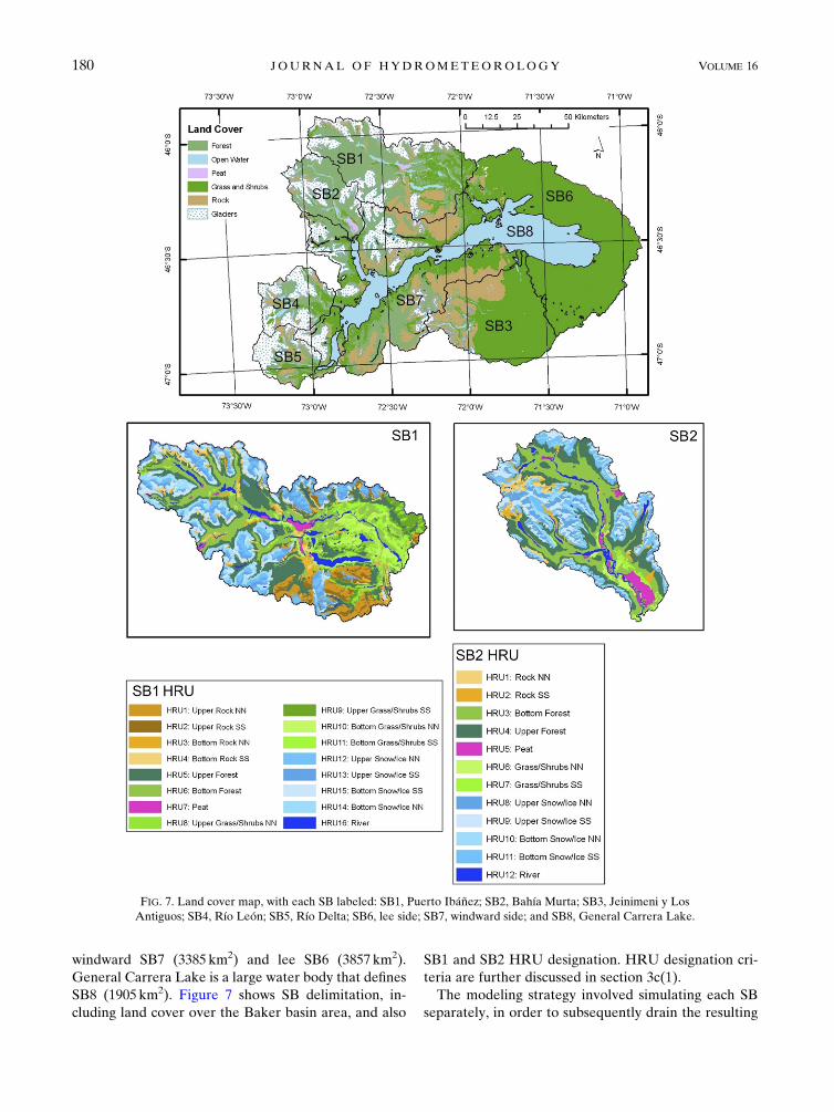
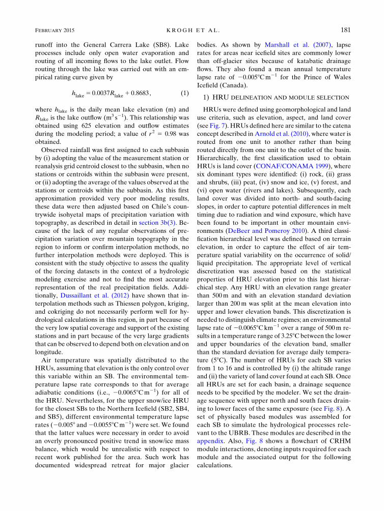
windward SB7 (3385 km2) and lee SB6 (3857 km2).
General Carrera Lake is a large water body that defines
SB8 (1905 km2). Figure 7 shows SB delimitation, in-
cluding land cover over the Baker basin area, and also
SB1 and SB2 HRU designation. HRU designation cri-
teria are further discussed in section 3c(1).
The modeling strategy involved simulating each SB
separately, in order to subsequently drain the resulting
FIG. 7. Land cover map, with each SB labeled: SB1, Puerto Ibáñez; SB2, Bahía Murta; SB3, Jeinimeni y LosAntiguos; SB4, Río León; SB5, Río Delta; SB6, lee side; SB7, windward side; and SB8, General Carrera Lake.
180 JOURNAL OF HYDROMETEOROLOGY VOLUME 16
runoff into the General Carrera Lake (SB8). Lake
processes include only open water evaporation and
routing of all incoming flows to the lake outlet. Flow
routing through the lake was carried out with an em-
pirical rating curve given by
hlake5 0:0037Rlake1 0:8683, (1)
where hlake is the daily mean lake elevation (m) and
Rlake is the lake outflow (m3 s21). This relationship was
obtained using 625 elevation and outflow estimates
during the modeling period; a value of r2 5 0.98 was
obtained.
Observed rainfall was first assigned to each subbasin
by (i) adopting the value of the measurement station or
reanalysis grid centroid closest to the subbasin, when no
stations or centroids within the subbasin were present,
or (ii) adopting the average of the values observed at the
stations or centroids within the subbasin. As this first
approximation provided very poor modeling results,
these data were then adjusted based on Chile’s coun-
trywide isohyetal maps of precipitation variation with
topography, as described in detail in section 3b(3). Be-
cause of the lack of any regular observations of pre-
cipitation variation over mountain topography in the
region to inform or confirm interpolation methods, no
further interpolation methods were deployed. This is
consistent with the study objective to assess the quality
of the forcing datasets in the context of a hydrologic
modeling exercise and not to find the most accurate
representation of the real precipitation fields. Addi-
tionally, Dussaillant et al. (2012) have shown that in-
terpolation methods such as Thiessen polygon, kriging,
and cokriging do not necessarily perform well for hy-
drological calculations in this region, in part because of
the very low spatial coverage and support of the existing
stations and in part because of the very large gradients
that can be observed to depend both on elevation and on
longitude.
Air temperature was spatially distributed to the
HRUs, assuming that elevation is the only control over
this variable within an SB. The environmental tem-
perature lapse rate corresponds to that for average
adiabatic conditions (i.e., 20.00658Cm21) for all of
the HRU. Nevertheless, for the upper snow/ice HRU
for the closest SBs to the Northern Icefield (SB2, SB4,
and SB5), different environmental temperature lapse
rates (20.0058 and20.00558Cm21) were set. We found
that the latter values were necessary in order to avoid
an overly pronounced positive trend in snow/ice mass
balance, which would be unrealistic with respect to
recent work published for the area. Such work has
documented widespread retreat for major glacier
bodies. As shown by Marshall et al. (2007), lapse
rates for areas near icefield sites are commonly lower
than off-glacier sites because of katabatic drainage
flows. They also found a mean annual temperature
lapse rate of 20.0058Cm21 for the Prince of Wales
Icefield (Canada).
1) HRU DELINEATION AND MODULE SELECTION
HRUs were defined using geomorphological and land
use criteria, such as elevation, aspect, and land cover
(see Fig. 7). HRUs defined here are similar to the catena
concept described in Arnold et al. (2010), where water is
routed from one unit to another rather than being
routed directly from one unit to the outlet of the basin.
Hierarchically, the first classification used to obtain
HRUs is land cover (CONAF/CONAMA 1999), where
six dominant types were identified: (i) rock, (ii) grass
and shrubs, (iii) peat, (iv) snow and ice, (v) forest, and
(vi) open water (rivers and lakes). Subsequently, each
land cover was divided into north- and south-facing
slopes, in order to capture potential differences in melt
timing due to radiation and wind exposure, which have
been found to be important in other mountain envi-
ronments (DeBeer and Pomeroy 2010). A third classi-
fication hierarchical level was defined based on terrain
elevation, in order to capture the effect of air tem-
perature spatial variability on the occurrence of solid/
liquid precipitation. The appropriate level of vertical
discretization was assessed based on the statistical
properties of HRU elevation prior to this last hierar-
chical step. Any HRU with an elevation range greater
than 500m and with an elevation standard deviation
larger than 200m was split at the mean elevation into
upper and lower elevation bands. This discretization is
needed to distinguish climate regimes; an environmental
lapse rate of 20.00658Ckm21 over a range of 500m re-
sults in a temperature range of 3.258C between the lower
and upper boundaries of the elevation band, smaller
than the standard deviation for average daily tempera-
ture (58C). The number of HRUs for each SB varies
from 1 to 16 and is controlled by (i) the altitude range
and (ii) the variety of land cover found at each SB. Once
all HRUs are set for each basin, a drainage sequence
needs to be specified by the modeler. We set the drain-
age sequence with upper north and south faces drain-
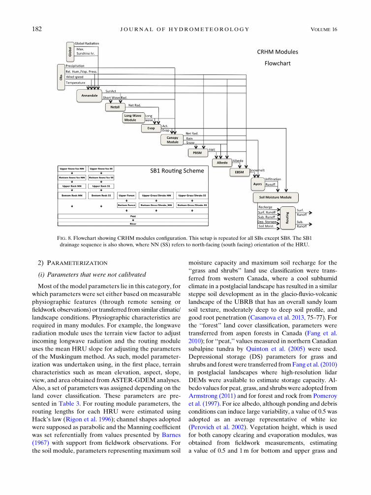
ing to lower faces of the same exposure (see Fig. 8). A
set of physically based modules was assembled for
each SB to simulate the hydrological processes rele-
vant to the UBRB. These modules are described in the
appendix. Also, Fig. 8 shows a flowchart of CRHM
module interactions, denoting inputs required for each
module and the associated output for the following
calculations.
FEBRUARY 2015 KROGH ET AL . 181
2) PARAMETERIZATION
(i) Parameters that were not calibrated
Most of themodel parameters lie in this category, for
which parameters were set either based on measurable
physiographic features (through remote sensing or
fieldworkobservations) or transferred fromsimilar climatic/
landscape conditions. Physiographic characteristics are
required in many modules. For example, the longwave
radiation module uses the terrain view factor to adjust
incoming longwave radiation and the routing module
uses the mean HRU slope for adjusting the parameters
of the Muskingum method. As such, model parameter-
ization was undertaken using, in the first place, terrain
characteristics such as mean elevation, aspect, slope,
view, and area obtained fromASTER-GDEM analyses.
Also, a set of parameters was assigned depending on the
land cover classification. These parameters are pre-
sented in Table 3. For routing module parameters, the
routing lengths for each HRU were estimated using
Hack’s law (Rigon et al. 1996); channel shapes adopted
were supposed as parabolic and the Manning coefficient
was set referentially from values presented by Barnes
(1967) with support from fieldwork observations. For
the soil module, parameters representing maximum soil
moisture capacity and maximum soil recharge for the
‘‘grass and shrubs’’ land use classification were trans-
ferred from western Canada, where a cool subhumid
climate in a postglacial landscape has resulted in a similar
steppe soil development as in the glacio-fluvio-volcanic
landscape of the UBRB that has an overall sandy loam
soil texture, moderately deep to deep soil profile, and
good root penetration (Casanova et al. 2013, 75–77). For
the ‘‘forest’’ land cover classification, parameters were
transferred from aspen forests in Canada (Fang et al.
2010); for ‘‘peat,’’ values measured in northern Canadian
subalpine tundra by Quinton et al. (2005) were used.
Depressional storage (DS) parameters for grass and
shrubs and forest were transferred fromFang et al. (2010)
in postglacial landscapes where high-resolution lidar
DEMs were available to estimate storage capacity. Al-
bedo values for peat, grass, and shrubswere adopted from
Armstrong (2011) and for forest and rock from Pomeroy
et al. (1997). For ice albedo, although ponding and debris
conditions can induce large variability, a value of 0.5 was
adopted as an average representative of white ice
(Perovich et al. 2002). Vegetation height, which is used
for both canopy clearing and evaporation modules, was
obtained from fieldwork measurements, estimating
a value of 0.5 and 1m for bottom and upper grass and
FIG. 8. Flowchart showing CRHM modules configuration. This setup is repeated for all SBs except SB8. The SB1
drainage sequence is also shown, where NN (SS) refers to north-facing (south facing) orientation of the HRU.
182 JOURNAL OF HYDROMETEOROLOGY VOLUME 16
shrubs and 6–12m for bottom and upper forest. For snow
transport and blowing snow sublimation, given that no us-
able in situ wind information was available for this study,
we adopted wind direction and velocity values from ERA-
Interim for themodel forcedwith otherwisemeasureddata.
For wind direction, both reanalyses confirm that the prin-
cipal direction during the modeling period was northwest.
Precipitation phase classification is based on a mean day
temperature index. As the model is set, when temperature
rises above 28C, precipitation is set as liquid, whereas below08C it is set as snowfall; for intermediate temperatures, the
precipitation phase was linearly interpolated.
(ii) Calibrated parameters and calibrationprocedure
Only two soil moisture parameters and the storage–
discharge rating curve relationship for General Carrera
Lake were calibrated manually, with the objective of
maximizing the NS coefficient criterion applied to daily
flows. DS parameters for rock, glaciers, and peat and
daily subsurface drainage (SSD) from recharge and soil
column for grass and shrubs, forest, and peat were cali-
brated, assuming the same value for each HRU type.
Calibration was carried out by analyzing the results of
the SB1 submodel, forced with CFSR data, with the
objective of maximizing the NS coefficient value com-
puted against observed daily streamflow data. The cali-
bration procedure is as follows. First, for several
arbitrary (within a realistic range) values of SSD, the DS
value was tested over the 5–300-mm range. This exercise
showed that the model has very little sensitivity to DS,
with NS changes smaller than 0.01 for each SSD value.
With this, an arbitrary but realistic value of DS 5 5mm
was set for rock, glaciers, and peat. Second, with the DS
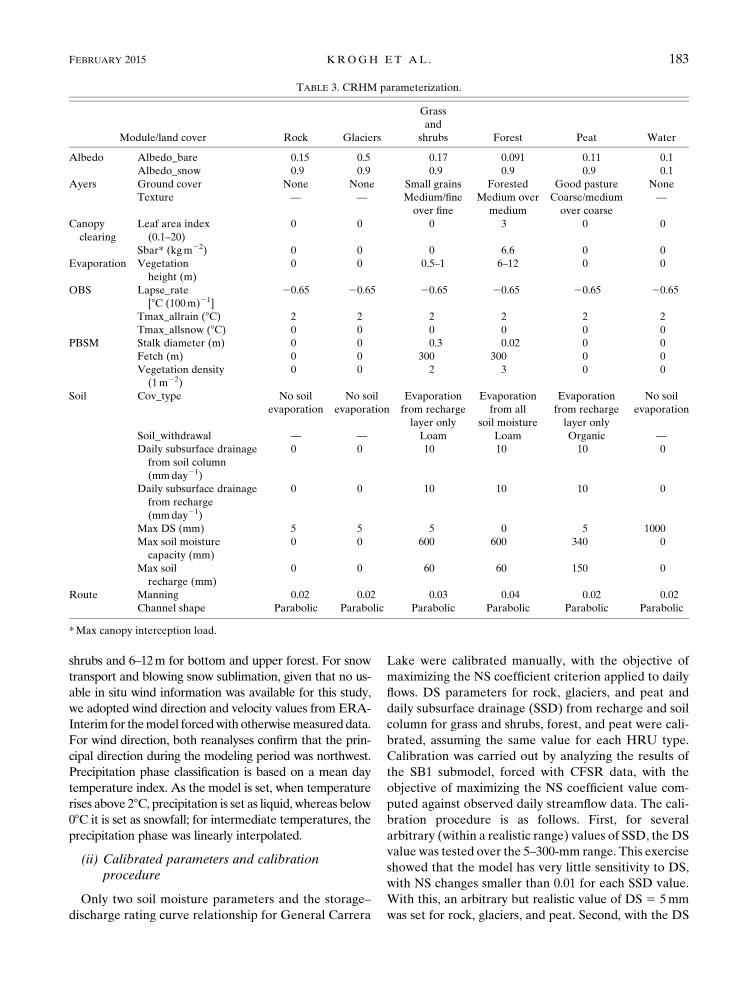
TABLE 3. CRHM parameterization.
Module/land cover Rock Glaciers
Grass
and
shrubs Forest Peat Water
Albedo Albedo_bare 0.15 0.5 0.17 0.091 0.11 0.1
Albedo_snow 0.9 0.9 0.9 0.9 0.9 0.1
Ayers Ground cover None None Small grains Forested Good pasture None
Texture — — Medium/fine
over fine
Medium over
medium
Coarse/medium
over coarse
—
Canopy
clearing
Leaf area index
(0.1–20)
0 0 0 3 0 0
Sbar* (kgm22) 0 0 0 6.6 0 0
Evaporation Vegetation
height (m)
0 0 0.5–1 6–12 0 0
OBS Lapse_rate
[8C (100m)21]
20.65 20.65 20.65 20.65 20.65 20.65
Tmax_allrain (8C) 2 2 2 2 2 2
Tmax_allsnow (8C) 0 0 0 0 0 0
PBSM Stalk diameter (m) 0 0 0.3 0.02 0 0
Fetch (m) 0 0 300 300 0 0
Vegetation density
(1m22)
0 0 2 3 0 0
Soil Cov_type No soil
evaporation
No soil
evaporation
Evaporation
from recharge
layer only
Evaporation
from all
soil moisture
Evaporation
from recharge
layer only
No soil
evaporation
Soil_withdrawal — — Loam Loam Organic —
Daily subsurface drainage
from soil column
(mmday21)
0 0 10 10 10 0
Daily subsurface drainage
from recharge
(mmday21)
0 0 10 10 10 0
Max DS (mm) 5 5 5 0 5 1000
Max soil moisture
capacity (mm)
0 0 600 600 340 0
Max soil
recharge (mm)
0 0 60 60 150 0
Route Manning 0.02 0.02 0.03 0.04 0.02 0.02
Channel shape Parabolic Parabolic Parabolic Parabolic Parabolic Parabolic
*Max canopy interception load.
FEBRUARY 2015 KROGH ET AL . 183
parameter value set, the SSDparameterwas tested again in
a more selective probable range of 1–20mmday21. These
runs showed that the model has a somewhat stronger sen-
sitivity to this parameter; for small values (1–4mmday21),
the NS coefficient varied around 0.3–0.5. For higher SSD
values (5–20mmday21), the model showed a smaller sen-
sitivity, but the best NS values between 0.5 and 0.53 were
also attained. Therefore, an arbitrary 10mmday21 mid-
point value within the ‘‘insensitive’’ range was selected.
Third, the insensitivity of theDSparameterwas verified for
the selected SSD value, thus finalizing the calibration stage.
(iii) Sensitivity analysis and insights
Calibrationwas also conductedusingobserved andERA-
Interim forcing data; however, using ‘‘optimal’’ parameters
from each forcing data source revealed that CFSR always
resulted in the best performance against streamflow obser-
vations; also, the parameter selection for these forcing data
are very similar to those found for CFRS (the model is in-
sensitive to DS, and optimal SSD values of 3 and
6mmday21 were obtained for ERA-Interim and observed
data, respectively). The calibration and parameter transfer
method used here corresponds to the deduction–induction–
abduction approach recommendedbyPomeroy et al. (2013)
for designing and parameterizing models for prediction in
ungauged basins. Physically based model parameter trans-
ference across .1000km between similar ecozones was
demonstrated by Dornes et al. (2008) in northern Canada
and by Gelfan et al. (2004) between Canada and Russia.
Because of the lack of any kind of detailed (i.e., finescale)
hydrological information for this basin, we chose to transfer
previously published parameter values whenever plausible
in order to minimize calibration. We find that, after this
process, only subsurface drainage and depression storage
parameters require calibration, which is seen here as
a promising result in terms of preserving a parsimonious
model in a relatively large, complex hydrological system.
3) PRECIPITATION DATA CORRECTION
Initial test model runs revealed important discrepancies
(bias) between observed and simulated runoff when forc-
ing the model with either observed or reanalysis data. This
bias problem has been found in other studies, such as
that developed by Pan et al. (2003), where they compare
SWE from four land surface models [Noah, Mosaic,
Sacramento Soil Moisture Accounting (SAC-SMA),
and Variable Infiltration Capacity (VIC)] against 3
years of Snow Telemetry (SNOTEL)-measured data.
Experiments with the VIC model indicated that most of
the bias in SWE is removed by scaling the precipitation
by a regional factor based on the regression of the North
American Land Data Assimilation System (NLDAS)
and SNOTEL-measured precipitation.
We attempted to mitigate the bias problem by estimat-
ing a precipitation correction factor (PCF) for adjusting
daily precipitation throughout the modeling period. Cor-
rection factors for precipitation input to gauged SB1 and
SB2 were estimated using the following expression:
PCFi115Robs
Rsim,i(PCF)i, (2)
where Robs is observed flow volume (m3) for the modeling
period and Rsim,i is simulated flow volume (m3) for each
model run i, which depends on the previous PCF calculated.
A manual iterative procedure allowed us to approximate
the most adequate correction factor, and the stopping cri-
terionwas set at bias#1%over the entiremodeling period.
Although it is very likely that a similar bias problem
affects the simulation of ungauged SBs, the lack of runoff
data, combined with the high spatial variability expected
for rainfall processes in this region, preclude our ability to
extrapolate PCFs specific for each SB from those esti-
mated for gauged basins. We circumvented this problem
by adopting the mean annual precipitation estimates
contained in Chile’s National Water Budget (DirecciónGeneral de Aguas 1987). The National Water Budget
contains mean annual precipitation isohyetal maps for the
entire country at a 1:1 000000 scale, estimated based on
observed streamflow and meteorological records; a sig-
nificant amount of expert inference and knowledge was
applied in deriving this product, and to date it remains the
sole source of nationwide water budget–related data. The
estimates take into account the likely spatial distribution
of precipitation due to orographic effects, as well as
basinwide evapotranspiration losses estimated through
the Turc–Pike relation. Mean annual precipitation and
potential ET are balanced by taking into account histori-
cal runoff datawhere available.Although crude, this is the
only additional source of annual rainfall data currently
available for this region aside from the meteorological
records and reanalyses already discussed. With this, the
PCF for ungauged SBs is estimated as follows:
PCF5Pp
PpNWB
, (3)
where Pp is total precipitation input from observations
or reanalyses and PpNWB is total precipitation from the
National Water Budget (mm). PCF values obtained
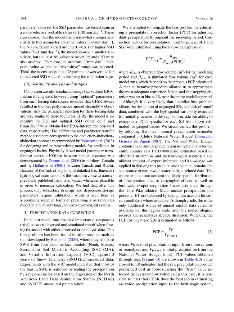
through Eqs. (2) and (3) are shown in Table 4. A value
closest to 1.0 indicates that the raw precipitation product
performed best in approximating the ‘‘true’’ value in-
ferred from streamflow volumes. In this case, it is pos-
sible to infer that CFSR does the best job in estimating
areawide precipitation input to the hydrologic system,
184 JOURNAL OF HYDROMETEOROLOGY VOLUME 16
whereas the observed record shows the largest bias, re-
quiring more than a twofold correction in order to ap-
proximate total water inputs to the basin.
4. Results and discussion
a. Model testing
We evaluate the performance of each input source by
comparing simulated streamflow at both gauged SBs
plus the outlet of General Carrera Lake. Performance
statistics include the NS coefficient (Nash and Sutcliffe
1970), root-mean-square error (RMSE) and bias:
NS5 12�(x0 2 xs)
2
�(x02 x0)2, (4)
RMSE5
ffiffiffiffiffiffiffiffiffiffiffiffiffiffiffiffiffiffiffiffiffiffiffiffiffiffiffiffiffi�n
i51
(x0,i 2 xs,i)2
n
vuuut, (5)
and
BIAS5�xs
�x02 1, (6)
where x0, xs, x, and n are observed, simulated,mean of the
observed values, and total number of values, respectively.
Large differences were found for every data source
and SB (see Table 5). In general, model performance
was enhanced when forcing CRHM with reanalyses in-
stead of observed data, especially for the entire Baker
basin, where the differences are more significant. The
well-established calibrated relationship between lake
level and outlet runoff can explain, in part, the satis-
factory results associated with Baker basin model
performance. This relationship constrains the range of
possible discharge values, attenuating peak flows due to
the substantial storage in the lake. The best performance
in SB1 and SB2 discharge was when CHRM was forced
with CFSR precipitation. This can be explained through
the CFSR spatial resolution, which, as shown in Fig. 4, is
3 times higher than that of the ERA-Interim and many
times the meteorological station density. In particular,
the representation of spatially variable meteorological
conditions within SB2 is crucial for model performance,
whereas for SB1, basin average weather conditions are
well correlated with SB1 observed outflow. This can be
explained by higher meteorological variability in SB2
due to the effect of the Northern Icefield in dampening
temperature lapse rates in its vicinity (Marshall et al.
2007). Such high variability in local hydrometeorology
suggests that a higher spatial resolution reanalysis like
CFSR should provide better results. ERA-Interim has
only one centroid within the Baker basin, and so its
representativeness is lower than that of CFSR.
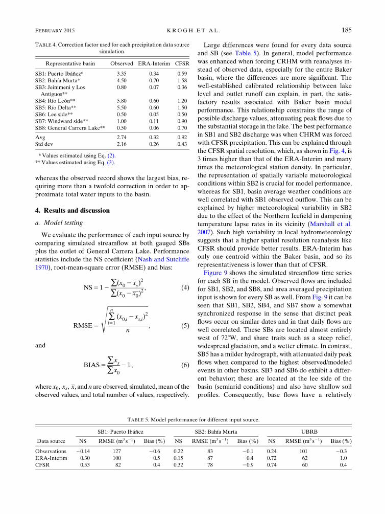
Figure 9 shows the simulated streamflow time series
for each SB in the model. Observed flows are included
for SB1, SB2, and SB8, and area averaged precipitation
input is shown for every SB as well. From Fig. 9 it can be
seen that SB1, SB2, SB4, and SB7 show a somewhat
synchronized response in the sense that distinct peak
flows occur on similar dates and in that daily flows are
well correlated. These SBs are located almost entirely
west of 728W, and share traits such as a steep relief,
widespread glaciation, and a wetter climate. In contrast,
SB5 has amilder hydrograph, with attenuated daily peak
flows when compared to the highest observed/modeled
events in other basins. SB3 and SB6 do exhibit a differ-
ent behavior; these are located at the lee side of the
basin (semiarid conditions) and also have shallow soil
profiles. Consequently, base flows have a relatively
TABLE 4. Correction factor used for each precipitation data source
simulation.
Representative basin Observed ERA-Interim CFSR
SB1: Puerto Ibáñez* 3.35 0.34 0.59
SB2: Bahía Murta* 4.50 0.70 1.58
SB3: Jeinimeni y Los
Antiguos**
0.80 0.07 0.36
SB4: Río León** 5.80 0.60 1.20
SB5: Río Delta** 5.50 0.60 1.50
SB6: Lee side** 0.50 0.05 0.50
SB7: Windward side** 1.00 0.11 0.90
SB8: General Carrera Lake** 0.50 0.06 0.70
Avg 2.74 0.32 0.92
Std dev 2.16 0.26 0.43
*Values estimated using Eq. (2).
**Values estimated using Eq. (3).
TABLE 5. Model performance for different input source.
Data source
SB1: Puerto Ibáñez SB2: Bahía Murta UBRB
NS RMSE (m3 s21) Bias (%) NS RMSE (m3 s21) Bias (%) NS RMSE (m3 s21) Bias (%)
Observations 20.14 127 20.6 0.22 83 20.1 0.24 101 20.3
ERA-Interim 0.30 100 20.5 0.15 87 20.4 0.72 62 1.0
CFSR 0.53 82 0.4 0.32 78 20.9 0.74 60 0.4
FEBRUARY 2015 KROGH ET AL . 185
small influence over the hydrograph. Although it is not
possible to corroborate the model results for the un-
gauged basins, Fig. 9 illustrates the potential of the
CFSR, in that it can actually predict a different climatic
regime, which in turn can be associated with a different
predicted hydrological response.
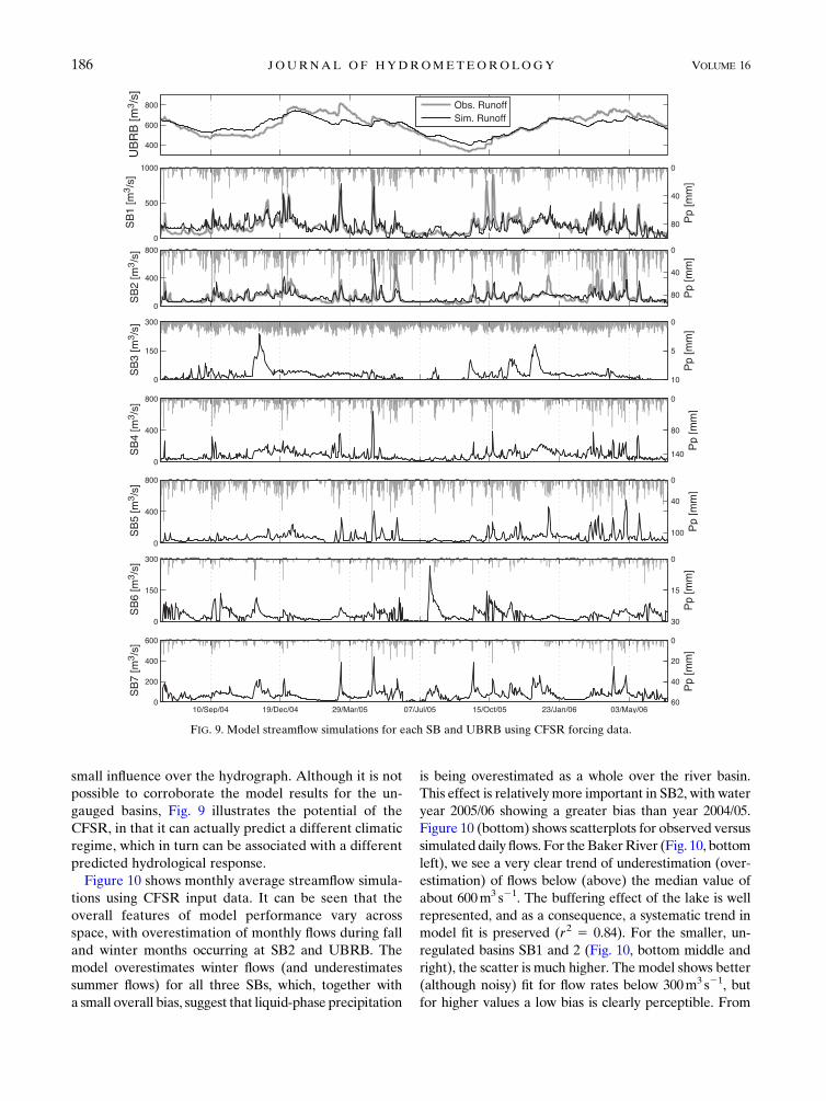
Figure 10 shows monthly average streamflow simula-
tions using CFSR input data. It can be seen that the
overall features of model performance vary across
space, with overestimation of monthly flows during fall
and winter months occurring at SB2 and UBRB. The
model overestimates winter flows (and underestimates
summer flows) for all three SBs, which, together with
a small overall bias, suggest that liquid-phase precipitation
is being overestimated as a whole over the river basin.
This effect is relativelymore important in SB2, with water
year 2005/06 showing a greater bias than year 2004/05.
Figure 10 (bottom) shows scatterplots for observed versus
simulated daily flows. For theBakerRiver (Fig. 10, bottom
left), we see a very clear trend of underestimation (over-
estimation) of flows below (above) the median value of
about 600m3 s21. The buffering effect of the lake is well
represented, and as a consequence, a systematic trend in
model fit is preserved (r2 5 0.84). For the smaller, un-
regulated basins SB1 and 2 (Fig. 10, bottom middle and
right), the scatter is much higher. The model shows better
(although noisy) fit for flow rates below 300m3 s21, but
for higher values a low bias is clearly perceptible. From
FIG. 9. Model streamflow simulations for each SB and UBRB using CFSR forcing data.
186 JOURNAL OF HYDROMETEOROLOGY VOLUME 16
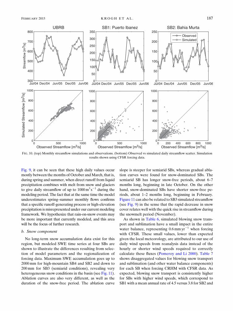
Fig. 9, it can be seen that these high daily values occur
mostly between themonths ofOctober andMarch, that is,
during spring and summer, when direct runoff from liquid
precipitation combines with melt from snow and glaciers
to give daily streamflow of up to 1000m3 s21 during the
modeling period. The fact that at the same time themodel
underestimates spring–summer monthly flows confirms
that a specific runoff-generating process or high-elevation
precipitation ismisrepresented under our currentmodeling
framework. We hypothesize that rain-on-snow events may
be more important that currently modeled, and this area
will be the focus of further research.
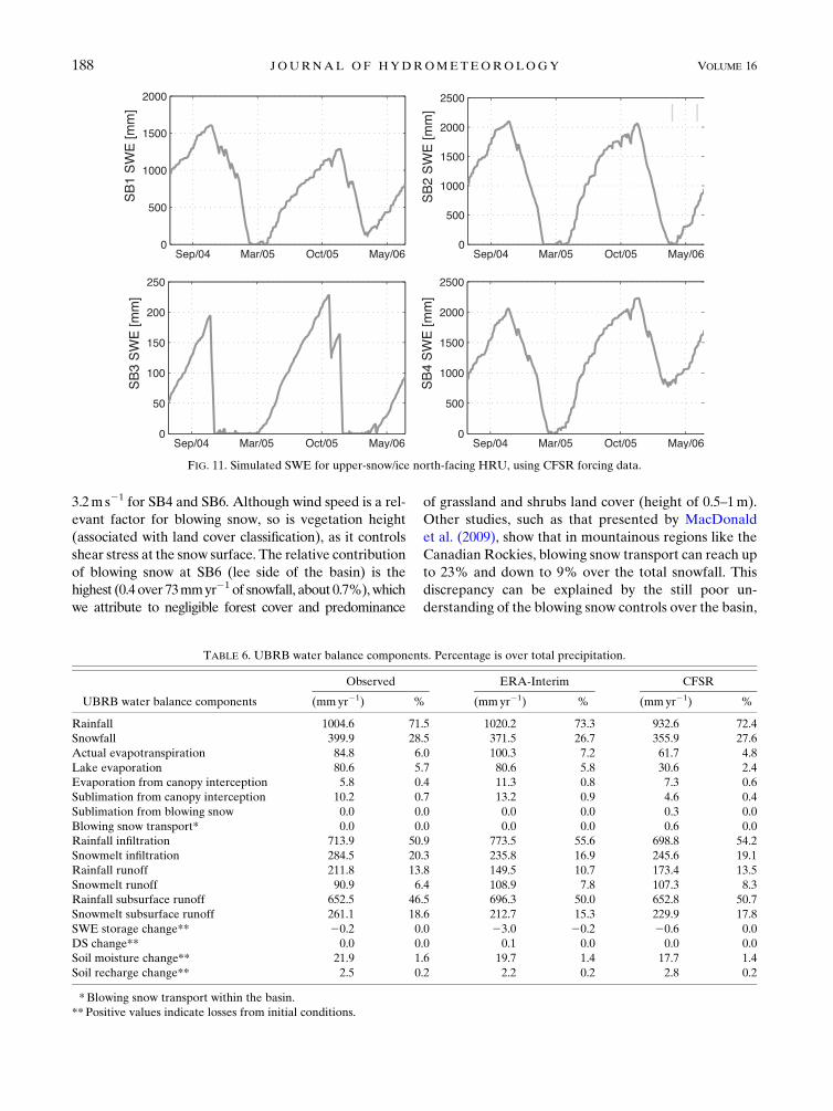
b. Snow component
No long-term snow accumulation data exist for this
region, but modeled SWE time series at four SBs are
shown to illustrate the differences resulting from selec-
tion of model parameters and the regionalization of
forcing data. Maximum SWE accumulation goes up to
2000mm for high-mountain SB4 and SB2 and down to
200mm for SB3 (semiarid conditions), revealing very
heterogeneous snow conditions in the basin (see Fig. 11).
Ablation curves are also very different, as well as the
duration of the snow-free period. The ablation curve
slope is steeper for semiarid SBs, whereas gradual abla-
tion curves were found for snow-dominated SBs. The
semiarid SB has longer snow-free periods, about 6–7
months long, beginning in late October. On the other
hand, snow-dominated SBs have shorter snow-free pe-
riods, about 1–2 months long, beginning in February.
Figure 11 can also be related to SB3 simulated streamflow
(see Fig. 9) in the sense that the rapid decrease in snow
cover relates well with the quick rise in streamflow during
the snowmelt period (November).
As shown in Table 6, simulated blowing snow trans-
port and sublimation have a small impact in the entire
water balance, representing 0.6mmyr21 when forcing
with CFSR. These small values, lower than expected
given the local meteorology, are attributed to our use of
daily wind speeds from reanalysis data instead of the
hourly or shorter wind speeds required to correctly
calculate these fluxes (Pomeroy and Li 2000). Table 7
shows disaggregated values for blowing snow transport
and sublimation (and other water balance components)
for each SB when forcing CRHM with CFSR data. As
expected, blowing snow transport is consistently higher
for SBs with higher wind speeds, which correspond to
SB1 with amean annual rate of 4.5 versus 3.8 for SB2 and
FIG. 10. (top) Monthly streamflow simulations and observations. (bottom) Observed vs simulated daily streamflow scatter. Simulation
results shown using CFSR forcing data.
FEBRUARY 2015 KROGH ET AL . 187
3.2m s21 for SB4 and SB6. Although wind speed is a rel-
evant factor for blowing snow, so is vegetation height
(associated with land cover classification), as it controls
shear stress at the snow surface. The relative contribution
of blowing snow at SB6 (lee side of the basin) is the
highest (0.4 over 73mmyr21 of snowfall, about 0.7%),which
we attribute to negligible forest cover and predominance
of grassland and shrubs land cover (height of 0.5–1m).
Other studies, such as that presented by MacDonald
et al. (2009), show that in mountainous regions like the
Canadian Rockies, blowing snow transport can reach up
to 23% and down to 9% over the total snowfall. This
discrepancy can be explained by the still poor un-
derstanding of the blowing snow controls over the basin,
FIG. 11. Simulated SWE for upper-snow/ice north-facing HRU, using CFSR forcing data.
TABLE 6. UBRB water balance components. Percentage is over total precipitation.
UBRB water balance components
Observed ERA-Interim CFSR
(mmyr21) % (mmyr21) % (mmyr21) %
Rainfall 1004.6 71.5 1020.2 73.3 932.6 72.4
Snowfall 399.9 28.5 371.5 26.7 355.9 27.6
Actual evapotranspiration 84.8 6.0 100.3 7.2 61.7 4.8
Lake evaporation 80.6 5.7 80.6 5.8 30.6 2.4
Evaporation from canopy interception 5.8 0.4 11.3 0.8 7.3 0.6
Sublimation from canopy interception 10.2 0.7 13.2 0.9 4.6 0.4
Sublimation from blowing snow 0.0 0.0 0.0 0.0 0.3 0.0
Blowing snow transport* 0.0 0.0 0.0 0.0 0.6 0.0
Rainfall infiltration 713.9 50.9 773.5 55.6 698.8 54.2
Snowmelt infiltration 284.5 20.3 235.8 16.9 245.6 19.1
Rainfall runoff 211.8 13.8 149.5 10.7 173.4 13.5
Snowmelt runoff 90.9 6.4 108.9 7.8 107.3 8.3
Rainfall subsurface runoff 652.5 46.5 696.3 50.0 652.8 50.7
Snowmelt subsurface runoff 261.1 18.6 212.7 15.3 229.9 17.8
SWE storage change** 20.2 0.0 23.0 20.2 20.6 0.0
DS change** 0.0 0.0 0.1 0.0 0.0 0.0
Soil moisture change** 21.9 1.6 19.7 1.4 17.7 1.4
Soil recharge change** 2.5 0.2 2.2 0.2 2.8 0.2
*Blowing snow transport within the basin.
** Positive values indicate losses from initial conditions.
188 JOURNAL OF HYDROMETEOROLOGY VOLUME 16
compounded with the lack of appropriate wind speed
data, which cannot be compared or adjusted with any
measurement within the basin. A site visit in October
2012 suggested substantial blowing snow transport in
alpine areas after snowfall events.
Notwithstanding the high ice depletion rates found for
the NPIF, up to 4.06 0.97myr21 (Rivera et al. 2007) for
the period between 1975 and 2001, no streamflow trend
can be seen for the period 1991–2008 at the UBRB. This
fact suggests that this depletion rate over the small
portion of the NPIF within this basin has limited in-
fluence for the runoff generation process.
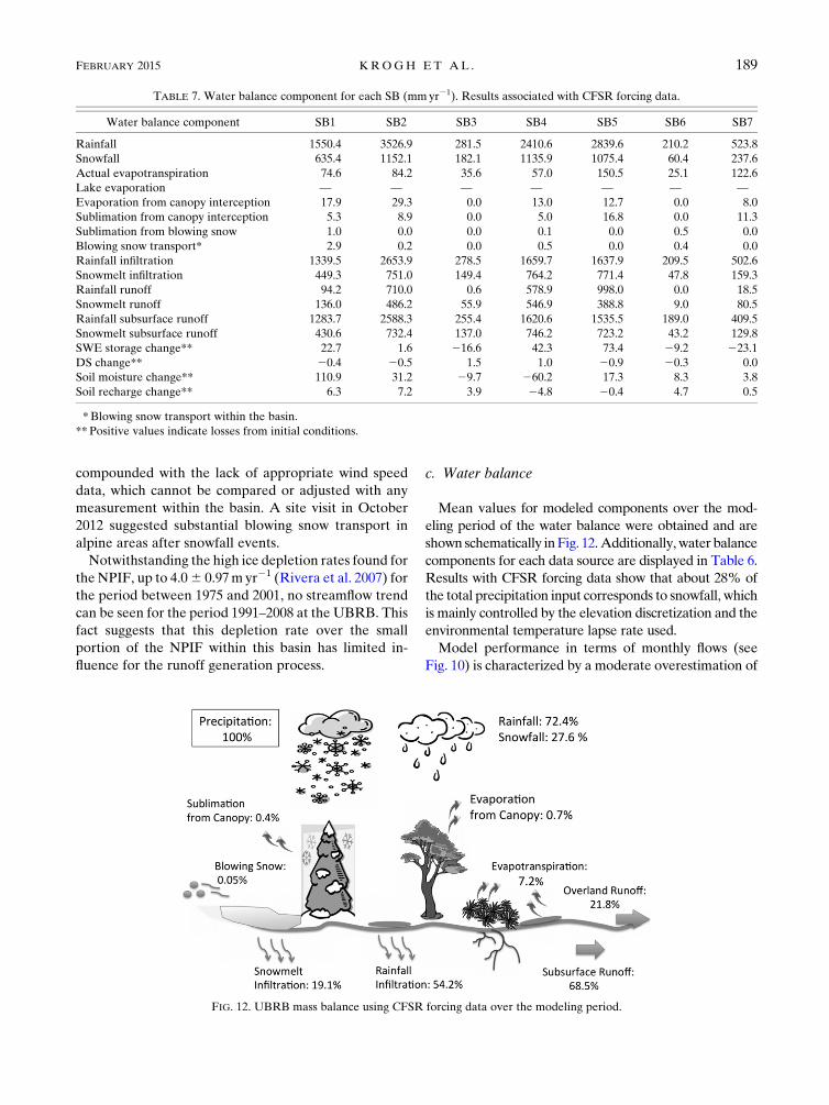
c. Water balance
Mean values for modeled components over the mod-
eling period of the water balance were obtained and are
shown schematically inFig. 12.Additionally, water balance
components for each data source are displayed in Table 6.
Results with CFSR forcing data show that about 28% of
the total precipitation input corresponds to snowfall, which
is mainly controlled by the elevation discretization and the
environmental temperature lapse rate used.
Model performance in terms of monthly flows (see
Fig. 10) is characterized by a moderate overestimation of
TABLE 7. Water balance component for each SB (mmyr21). Results associated with CFSR forcing data.
Water balance component SB1 SB2 SB3 SB4 SB5 SB6 SB7
Rainfall 1550.4 3526.9 281.5 2410.6 2839.6 210.2 523.8
Snowfall 635.4 1152.1 182.1 1135.9 1075.4 60.4 237.6
Actual evapotranspiration 74.6 84.2 35.6 57.0 150.5 25.1 122.6
Lake evaporation — — — — — — —
Evaporation from canopy interception 17.9 29.3 0.0 13.0 12.7 0.0 8.0
Sublimation from canopy interception 5.3 8.9 0.0 5.0 16.8 0.0 11.3
Sublimation from blowing snow 1.0 0.0 0.0 0.1 0.0 0.5 0.0
Blowing snow transport* 2.9 0.2 0.0 0.5 0.0 0.4 0.0
Rainfall infiltration 1339.5 2653.9 278.5 1659.7 1637.9 209.5 502.6
Snowmelt infiltration 449.3 751.0 149.4 764.2 771.4 47.8 159.3
Rainfall runoff 94.2 710.0 0.6 578.9 998.0 0.0 18.5
Snowmelt runoff 136.0 486.2 55.9 546.9 388.8 9.0 80.5
Rainfall subsurface runoff 1283.7 2588.3 255.4 1620.6 1535.5 189.0 409.5
Snowmelt subsurface runoff 430.6 732.4 137.0 746.2 723.2 43.2 129.8
SWE storage change** 22.7 1.6 216.6 42.3 73.4 29.2 223.1
DS change** 20.4 20.5 1.5 1.0 20.9 20.3 0.0
Soil moisture change** 110.9 31.2 29.7 260.2 17.3 8.3 3.8
Soil recharge change** 6.3 7.2 3.9 24.8 20.4 4.7 0.5
*Blowing snow transport within the basin.
**Positive values indicate losses from initial conditions.
FIG. 12. UBRB mass balance using CFSR forcing data over the modeling period.
FEBRUARY 2015 KROGH ET AL . 189
winter (low) flows and underestimation of high (summer)
flows, which in turn could be related by an overestimation
of the rainfall fraction of precipitation throughout the basin
during the winter months. Four reasons could explain this
behavior: (i) a high bias in the index temperature station/
reanalysis data used for spatial interpolation, (ii) a too-
shallow lapse rate or misrepresentation of its temporal
variability, (iii) overestimation of precipitation amounts at
lower elevations due to spatial averaging at the subbasin
scale, and (iv) inadequate selection of parameter values.
No reliable field data exist in order to test the above hy-
pothesis for the modeling period, so this topic constitutes
a relevant direction for future research. A recent im-
provement to CRHM for phase determination using
a psychrometric energy balance method (Harder and
Pomeroy 2013) holds promise for future evaluations of
precipitation phase if reliable humidity measurements
become available in the region.
In terms of runoff generation, we found that sub-
surface flow is significantly more important (68.5%) that
overland runoff (21.8%). This can be explained by the
high infiltration rates and soil moisture storage capacity,
especially for forested and peat land cover. Even though
modeled liquid-phase precipitation almost triples snow-
fall, little difference exists in terms of each precipitation
overland contribution; rainfall- and snowmelt-generated
overland flows contribute 13.5% and 8.3% to total flow,
respectively. Evapotranspiration, sublimation, and lake
evaporation take up to 8.2% of total precipitation,
with negligible contributions from canopy interception
losses (,1%). These evapotranspiration losses account
for about 100mmyr21, significantly different from the
351mmyr21 estimation contained in the Chilean Na-
tionalWater Budget (DirecciónGeneral deAguas 1987),which in turn amount to 20% of the then-estimated long-
term precipitation mean for the basin of 1686mmyr21.
Because our modeling period is drier than the reference
period in the Chilean Water Budget (approximately
1400mmyr21), it is expected that ET as a percentage of
annual precipitation would be different from the clima-
tological value. However, in theory, this percentage
should be larger, not smaller, than the reference one. The
lack of intermediate state variable information precludes
us from formulating a hypothesis with respect to the na-
ture of this discrepancy, and future research should aim at
developing point-scale water balances through lysimeter
experiments in order to obtain a better understanding of
water fluxes along the atmosphere–soil column in various
climatic regimes across this region.
Low interception sublimation losses are attributed to
the largely deciduous nature of the forest canopies, and
low evaporation and sublimation capacity are derived
from existing moist and cold conditions. Simulated
blowing snow has a negligible influence on the water
balance (as discussed in section 4b), and only when
the model is forced with CFSR input data is a small
amount of drifted snow transported from each HRU
(0.7mmyr21 on average). Storage change in the basin
results from SWE, soil moisture, depression storage, and
soil recharge changes. This component has little impact
on the modeling, only 1.6%; soil moisture changes rep-
resent the most relatively important change (1.4%).
Both SWE and depression storage changes are null.
Table 7 shows spatially disaggregated SB water bal-
ance components when CRHM is forced with CFSR.
Results show that the model is capable of simulating the
west–east precipitation gradient within the basin, with
high precipitation patterns over SB1, SB2, SB4, and
SB5, which total about 72% of the entire precipitation
over the basin, to the dry eastern patterns of SB6 and
SB3, which only total about 9% of total precipitation
input over the basin. Other differences can be high-
lighted, like evapotranspiration, where SB7 contributes
42% of the total evapotranspiration, with significant
forested land (about 1029 km2) and grassland and
shrubland (699 km2).
5. Conclusions
This paper presents the first insight into the hydro-
logical cycle and water balance of a Patagonian moun-
tain and lowland basin through physically based
modeling. Like most remote and sparsely populated
regions in SouthAmerica, Patagonia has a low density of
meteorological stations, many times with incomplete
and/or unreliable records. To circumvent this problem
and evaluate the impact of data scarcity, data from ob-
served local meteorological stations and reanalyses were
analyzed and then used as forcing data to the hydrologic
model. Actual meteorological stations have poor rep-
resentativeness over the Baker basin because (i) only
rainfall gauges are available, whereas snowfall events
are frequent and significant, and (ii) meteorological
stations are all located at low altitudes (,500m MSL),
neglecting higher precipitation magnitudes at higher
elevation due to orographic effects.
The performance of a CRHM for the Baker basin was
shown to be more satisfactory when forced with re-
analyses data, obtaining values ofNS. 0.7 for daily flows,
than when forced with weather station observations.
Because bias was mostly removed from all precipitation
forcings by a precipitation correction, the higher perfor-
mance of the model when forced with reanalysis data can
be in attributed in part to a better temporal representa-
tion of precipitation events, as the observation record
does not include snowfall, and also to better spatial
190 JOURNAL OF HYDROMETEOROLOGY VOLUME 16
averaging of precipitation when compared to point ob-
servations in valley bottoms. When evaluating the per-
formance of the hydrological model in individual
subbasins, CFSR proved to be a better estimator of local
meteorological conditions, which is reasonable since
CFSR has 3 times the spatial resolution of ERA-Interim
in this region. These results strongly indicate that re-
analysis data have great potential as an effective source of
information for hydrological understanding in ungauged
or poorly monitored basins, such as those located in Pa-
tagonia. Transferring some parameters from hydrological
studies in other cold regions ecosystems—in this case,
by abductive inference of certain parameters from
those developed in Canadian research basins—proved
to be a viable approach for this remote and poorly
gauged basin and allowed us to avoid or minimize
complex calibration schemes, obtaining satisfactory
results when no other local source of information was
available.
The model results suggest that, although snowfall was
only 28% of total precipitation, modeled snowmelt
contributed to streamflow for up to 6 months per year
and was the major source of runoff. This is not dissimilar
from the hydrology of many regions in western Canada
(Pomeroy et al. 2007). Infiltration was the principal
component in the water balance, capturing about 73%
of the total precipitation and showing the influence of
subsurface flow generation mechanisms. Some of the
infiltrated water remained in the basin until the next
hydrological year but most formed runoff. Evapotrans-
piration from soils and evaporation from lakes repre-
sented losses of only 8% of total precipitation, which is
half of the mean annual value estimated through simple
temperature-based equations in the Chilean Water
Budget. The differences are due to consideration of snow
cover suppression of evaporation and the deployment of
physically based combinationmethod evapotranspiration
and aerodynamic lake evaporation schemes in CRHM.
Evapotranspiration depends strongly on season, soil
moisture capacity, and vegetation, which are based on
land cover classification, and lake evaporation depends
on wind speed, relative humidity, andmean temperature.
Hence, the development of more accurate land cover
maps, as well as meteorological stations with wind speed
and relative humidity sensors, are crucial in order to ob-
tain more precise estimations for evaporative losses,
which should be validated against, for instance, lysimeter
experiments in representative locations.
Future research must seek finer-scale spatial repre-
sentations of mountain meteorology in the region that
better approach the HRU spatial discretization, starting
from the improved representation that the reanalyses—
CFSR, in particular—provide. Also, future research
must include refining the estimation of blowing snow
phenomena by acquiring finescale, subdaily wind speed
data, validating rain-on-snow energy exchanges through
point-based field experiments, and further refining the
contribution of the Northern Icefield to the hydrology of
the region, in view of current climate change pro-
jections, which indicate warming for the region and
a continued decrease in glacier ice storage.
Acknowledgments. The authors acknowledge the fi-
nancial support from Fondecyt Project 1090479, Grad-
uateDivision of theMathematical and Physical Sciences
Faculty, University of Chile, with their Grant ‘‘PasantíasCortas de Investigación’’; from NSERC Discovery
Grants, Canada Research Chairs; and from the Inter-
American Institute for Global Change Research (IAI)
under Grant SGP-CRA2047. The authors also thank the
Dirección General de Aguas (DGA), which provided allthe observed data used in this study. Sebastian Kroghalso thanks Xing Fang and Tom Brown for their im-portant advice on modeling strategies with CRHM.
APPENDIX
CRHM Modules Description
d Global calculates the theoretical global radiation and
direct and diffuse solar radiation, as well as maximum
sunshine hours based on latitude, elevation, ground
slope, and azimuth (Garnier and Ohmura 1970).d Annandale estimates incoming shortwave radiation
from daily minimum and maximum temperatures
(Annandale et al. 2001) and theoretical global radia-
tion from the ‘‘global’’ module.d The longwave radiation module estimates incoming
longwave radiation using temperature, humidity, and
shortwave transmittance (Sicart et al. 2006).d Albedo estimates snow albedo throughout the winter
and into themelt period. Albedo is estimated following
a linear decay rate for each time period based on snow
depth, new snow, and melting (temperature and radi-
ation criteria) occurrence (Gray and Landine 1987).d Netall models net all-wave radiation to snow-free
surfaces from the Brunt equation (Brunt 1932), using
inputs from the ‘‘global’’ and ‘‘Annandale’’ radiation
modules.d Prairie Blowing SnowModel (PBSM) calculates SWE
from snowfall and blowing snow transport, redistribu-
tion, and sublimation (Pomeroy and Li 2000).d Energy-Budget Snowmelt Model (EBSM) estimates
snowmelt by calculating the energy balance of radiation,
FEBRUARY 2015 KROGH ET AL . 191
sensible heat, latent heat, advection from rainfall, and
change in internal snowpack energy (Gray and Landine
1988).d Ayers is an empirical relationship that estimates
rainfall infiltration into unfrozen soils based on soil
texture and ground cover (Ayers 1959).d The evaporation module has two types: (i) Granger’s
evaporation expression (Granger and Gray 1989;
Granger and Pomeroy 1997) estimates actual evapo-
transpiration from unsaturated surfaces (canopy,
crops, soils) using a complementary solution to the
Penman equation, and (ii) the Priestley and Taylor
evaporation expression (Priestley and Taylor 1972)
estimates evaporation from saturated surfaces, wet-
lands, or small water bodies including advection
effects.d The canopymodule estimates the snowfall and rainfall
intercepted, sublimated, and evaporated by the forest
canopy, subcanopy snowfall, rainfall, and shortwave
and longwave radiation (Ellis et al. 2010).d The soil moisture module computes soil moisture
balance for frozen and unfrozen periods (Pomeroy
et al. 2007, 2012); moisture content exceeding field
capacity is routed away from the HRU using
‘‘netroute.’’d TheMuskingum routing module is based on a variable
discharge–storage relationship (Chow 1964) and is
used to route runoff between HRUs.d The lake evaporation module is an empirical relation-
ship that estimates monthly large lake actual evapo-
ration using monthly wind speed, relative humidity,
and temperature, following the Meyer formula with
coefficients as determined by the Prairie Provinces
Water Board in western Canada (Martin 2002).
REFERENCES
Annandale, J. G., N. Z. Jovanovic, N. Benadé, and R. G. Allen,
2001: Software for missing data error analysis of Penman–
Monteith reference evapotranspiration. Irrig. Sci., 21, 57–67,
doi:10.1007/s002710100047.
Aravena, J. C., 2007: Reconstructing climate variability using tree
rings and glaciers fluctuations in southern Chilean Andes.
Ph.D. thesis, Graduate Program in Geography, University of
Western Ontario, 220 pp.
Armstrong, R. N., 2011: Spatial variability of actual evapotrans-
piration in a prairie landscape. Ph.D. thesis, Dept. of Geog-
raphy and Planning, University of Saskatchewan, 194 pp.
Arnold, J. G., P. M. Allen, M. Volk, J. R. Williams, and D. D.
Bosch, 2010: Assessment of different representations of spa-
tial variability on SWATmodel performance. Trans. ASABE,
53, 1433–1443.Ayers, H. D., 1959: Influence of soil profile and vegetation char-
acteristics on net rainfall supply to runoff. Spillway Design
Floods: Proceedings of Hydrology SymposiumNo. 1,National
Research Council of Canada, 198–205. [Available online at
www.usask.ca/hydrology/papers/Ayers_1959.pdf.]
Barnes, H. H., 1967: Roughness characteristics of natural channels.
USGS Water Supply Paper 1849, 213 pp. [Available online at
http://pubs.usgs.gov/wsp/wsp_1849/.]
Barría, P. L., 2010: Pronóstico de Caudales Medios Mensuales enlas Cuencas de los Ríos Baker y Pascua. Civil engineeringthesis, Civil Engineering Dept., University of Chile, 167 pp.
Brunt, D., 1932: Notes on radiation in the atmosphere. Quart.
J. Roy. Meteor. Soc., 58, 389–420, doi:10.1002/qj.49705824704.Casanova, M., O. Salazar, O. Seguel, andW. Luzio, 2013: The Soils
of Chile. Springer, 185 pp.
Chow, V. T., 1964: Handbook of Applied Hydrology. McGraw-
Hill, 1468 pp.
CONAF/CONAMA, 1999: Catastro y evaluación de los recursosvegetacionales nativos de Chile. Project Rep., 89 pp. [Availableonline at www.bcn.cl/carpeta_temas_profundidad/ley-bosque-
nativo/archivos-pdf/Catastro.pdf.]
DeBeer, C. M., and J. W. Pomeroy, 2010: Simulation of the snow-
melt runoff contributing area in a small alpine basin. Hydrol.
Earth Syst. Sci., 14, 1205–1219, doi:10.5194/hess-14-1205-2010.Dee, D. P., and Coauthors, 2011: The ERA-Interim reanalysis:
Configuration andperformance of the data assimilation system.
Quart. J. Roy. Meteor. Soc., 137, 553–597, doi:10.1002/qj.828.
Dirección General de Aguas, 1987: Balance hidrológico nacional.Tech. Rep. 70115, Dirección General de Aguas, 62 pp.[Available online at http://documentos.dga.cl/SUP1540.pdf.]
Dornes, P. F., A. T. Bryan, B. Davison, A. Pietroniro, J. W.
Pomeroy, and P. Marsh, 2008: Regionalization of land surface
hydrological model parameters in subarctic environments. Phys.
Chem. Earth, 33, 1081–1089, doi:10.1016/j.pce.2008.07.007.
Dussaillant, J. A., W. Buytaert, C. Meier, and F. Espinoza, 2012:
Hydrological regime of remote catchments with extreme gra-
dients under accelerated change: The Baker basin in Patagonia.
Hydrol. Sci. J., 57, 1530–1542, doi:10.1080/02626667.2012.726993.Ellis, C. R., J. W. Pomeroy, T. Brown, and J. MacDonald, 2010:
Simulation of snow accumulation and melt in needleleaf forest
environments.Hydrol. Earth Syst. Sci., 14, 925–940, doi:10.5194/
hess-14-925-2010.
Fang, X., and J. W. Pomeroy, 2007: Snowmelt runoff sensitivity
analysis to drought on the Canadian prairies. Hydrol. Pro-
cesses, 21, 2594–2609, doi:10.1002/hyp.6796.
——, and ——, 2009: Modelling blowing snow redistribution to
prairie wetlands. Hydrol. Processes, 23, 2557–2569,
doi:10.1002/hyp.7348.
——, ——, C. J. Westbrook, X. Guo, A. G. Minke, and T. Brown,
2010: Prediction of snowmelt derived streamflow in a wetland
dominated prairie basin.Hydrol. Earth Syst. Sci., 14, 991–1006,
doi:10.5194/hess-14-991-2010.
——, ——, C. R. Ellis, M. K. MacDonald, C. M. DeBeer, and
T. Brown, 2013: Multi-variable evaluation of hydrological
model predictions for a headwater basin in the Canadian
Rocky Mountains. Hydrol. Earth Syst. Sci., 17, 1635–1659,
doi:10.5194/hess-17-1635-2013.
Garnier, B. J., and A. Ohmura, 1970: The evaluation of surface
variations in solar radiation income. Sol. Energy, 13, 21–34,
doi:10.1016/0038-092X(70)90004-6.
Garreaud, R., M. Vuille, R. Compagnucci, and J. Marengo, 2009:
Present-daySouthAmerican climate.Palaeogeogr.Palaeoclimatol.
Palaeoecol., 281, 180–195, doi:10.1016/j.palaeo.2007.10.032.
Gelfan, A. N., J. W. Pomeroy, and L. S. Kuchment, 2004:Modeling
forest cover influences on snow accumulation, sublimation
192 JOURNAL OF HYDROMETEOROLOGY VOLUME 16
and melt. J. Hydrometeor., 5, 785–803, doi:10.1175/
1525-7541(2004)005,0785:MFCIOS.2.0.CO;2.
Gonthier, C., 2011: Influencia de la escala espacial y representaciónhidrológica de una Cuenca de montaña sobre la capacidadpredictiva de un modelo hidrológico. M.S. thesis, Civil Engi-neering Dept., University of Chile, 165 pp.
Granger, R. J., and D. M. Gray, 1989: Evaporation from natural
non-saturated surfaces. J. Hydrol., 111, 21–29, doi:10.1016/0022-1694(89)90249-7.
——, and J. W. Pomeroy, 1997: Sustainability of the western Ca-
nadian boreal forest under changing hydrological conditions.
II. Summer energy and water use. IAHS Publ., 240, 243–249.[Available online at http://iahs.info/uploads/dms/iahs_240_
0243.pdf.]
Gray, D. M., and P. G. Landine, 1987: Albedo model for shallow
prairie snow covers.Can. J. Earth Sci., 24, 1760–1768, doi:10.1139/
e87-168.
——, and ——, 1988: An energy-budget snowmelt model for the
Canadian Prairies. Can. J. Earth Sci., 25, 1292–1303, doi:10.1139/e88-124.
Harder, P., and J. Pomeroy, 2013: Estimating precipitation phase
using a phycrometric energy balance method. Hydrol. Pro-
cesses, 27, 1901–1914, doi:10.1002/hyp.9799.Lopez, P., P. Sirguey, Y. Arnaud, B. Pouyaud, and P. Chevalier,
2008: Snow cover monitoring in the Northern Patagonia Ice-
field usingMODIS satellite images (2000–2006).Global Planet.
Change, 61, 103–116, doi:10.1016/j.gloplacha.2007.07.005.
MacDonald, M., J. Pomeroy, and A. Pietroniro, 2009: Parameter-
izing redistribution and sublimation of blowing snow for hy-
drological models: Test in a mountainous subartic catchment.
Hydrol. Processes, 23, 2570–2583, doi:10.1002/hyp.7356.
Marshall, S. J., M. Sharp, D. Burgess, and F. Anslow, 2007: Near-
surface-temperature lapse rates on the Prince of Wales Ice-
field, Ellesmere Island, Canada: Implications for regional
downscaling of temperature. Int. J. Climatol., 27, 385–398,
doi:10.1002/joc.1396.
Martin, F. R., 2002: Gross evaporation for the 30-year period
1971–2000 in the Canadian Prairies. Hydrology Rep. 143,
Agriculture and Agri-Food Canada Prairie Farm Reha-
bilitation Administration Technical Service, 35 pp.
NASA, cited 2014: ASTER Global Digital Elevation Model.
[Available online at http://gdem.ersdac.jspacesystems.or.jp/.]
Nash, J. E., and J. V. Sutcliffe, 1970: River flow forecasting through
conceptual models. Part I—A discussion of principles. J. Hy-
drol., 10, 282–290, doi:10.1016/0022-1694(70)90255-6.Pan, M., and Coauthors, 2003: Snow process modeling in the North
American Land Data Assimilation System (NLDAS):
2. Evaluation of model simulated snow water equivalent.
J. Geophys. Res., 108, 8850, doi:10.1029/2003JD003994.
Perovich, D. K., T. C. Grenfell, B. Light, and P. V. Hobbs, 2002:
Seasonal evolution of the albedo of multiyear Arctic sea ice.
J. Geophys. Res., 107, 8044, doi:10.1029/2000JC000438.Pomeroy, J.W., andL. Li, 2000: Prairie andArctic areal snow cover
mass balance using a blowing snow model. J. Geophys. Res.,
105, 26 619–26 634, doi:10.1029/2000JD900149.
——, R. J. Granger, A. Pietroniro, J. E. Elliott, B. Toth, and
N. Hedstrom, 1997: Hydrological pathways in the PrinceAlbert
Model Forest. Final Rep. to Prince Albert Model Forest Asso-
ciation, 220 pp. [Available online at www.pamodelforest.sk.ca/
pubs/PAMF3400.pdf.]
——, D. M. Gray, T. Brown, N. R. Hedstrom, W. L. Quinton, R. J.
Granger, and S. K. Carey, 2007: The cold regions hydrological
model: A platform for basing process representation and
model structure on physical evidence. Hydrol. Processes, 21,
2650–2667, doi:10.1002/hyp.6787.
——,X. Fang, and C. Ellis, 2012: Sensitivity of snowmelt hydrology
in Marmot Creek, Alberta, to forest cover disturbance. Hy-
drol. Processes, 26, 1891–1904, doi:10.1002/hyp.9248.
——, P. H. Whitfield, and C. Spence, Eds., 2013: Putting Prediction
in Ungauged Basins into Practice. IAHS, 362 pp.
Priestley, C.H.B., andR. J. Taylor, 1972:On the assessment of surface
heat flux and evaporation using large-scale parameters. Mon.
Wea. Rev., 100, 81–92, doi:10.1175/1520-0493(1972)100,0081:
OTAOSH.2.3.CO;2.
Quinton, W. L., T. Shirazi, S. K. Carey, and J. W. Pomeroy, 2005:
Soil water storage and active-layer development in a sub-alpine
tundra hillslope, southern Yukon Territory, Canada. Perma-
frost Periglacial Processes, 16, 369–382, doi:10.1002/ppp.543.
Rigon, R., I. Rodriguez-Iturbe, andA.Maritan, 1996: OnHack’s law.
Water Resour. Res., 32, 3367–3374, doi:10.1029/96WR02397.
Rivera, A., T. Benham,G. Casassa, J. Mabmer, and J. Dowdeswell,
2007: Ice elevation and areal changes of glaciers from the
Northern Patagonia Icefield, Chile.Global Planet. Change, 59,
126–137, doi:10.1016/j.gloplacha.2006.11.037.
Saha, S., and Coauthors, 2010: TheNCEPClimate Forecast System
Reanalysis. Bull. Amer. Meteor. Soc., 91, 1015–1057,
doi:10.1175/2010BAMS3001.1.
Sheffield, J., A. Ziegler, and E.Wood, 2004: Correction of the high-
latitude rain day anomaly in the NCEP–NCAR reanalysis for
land surface hydrological modeling. J. Climate, 17, 3814–3828,
doi:10.1175/1520-0442(2004)017,3814:COTHRD.2.0.CO;2.
Sicart, J. E., J. W. Pomeroy, R. L. Essery, and D. Bewley, 2006:
Incoming longwave radiation to melting snow: Observations,
sensitivity and estimations in northern environments. Hydrol.
Processes, 20, 3697–3708, doi:10.1002/hyp.6383.Silva, V., V. Kousky, and R. Higgins, 2011: Daily precipitation
statistics for South America: An intercomparison between
NCEP reanalyses and observations. J. Hydrometeor., 12, 101–
117, doi:10.1175/2010JHM1303.1.
Ward, E., W. Buytaert, L. Peaver, and H. Wheather, 2011: Eval-
uation of precipitation products over complex mountainous
terrain: A water resources perspective. Adv. Water Resour.,
34, 1222–1231, doi:10.1016/j.advwatres.2011.05.007.Warren, R., and D. Sugden, 1993: The Patagonia Icefield: A gla-
ciological review. Arct. Alp. Res., 25, 316–331, doi:10.2307/
1551915.
WMO, 1994: Guide to hydrological practices. 5th ed. WMO Publ.
164, 735 pp.
Zhou, J., J. W. Pomeroy, W. Zhang, G. Cheng, G. Wang, and
C. Chen, 2014: Simulating cold regions hydrological processes
using a modular model in the west of China. J. Hydrol., 509,
13–24, doi:10.1016/j.jhydrol.2013.11.013.
FEBRUARY 2015 KROGH ET AL . 193