Pilot Protection Based on Directional Detection

Master Thesis

By

Sepehr Sefidpour

Supervisors: Jianping Wang, ABB Corporate Research

Rujiroj Leelaruji, KTH School of Electrical Engineering

Examiner: Lennart Söder, KTH School of Electrical Engineering

XR-EE-ES 2009:009

Royal Institute of Technology Department of Electrical Engineering

Electrical Power Systems Stockholm 2009

Abstract Nowadays two main types of protection schemes widely used in protection of transmission lines are: distance protection and differential protection schemes. However, it has been noticed from industrial practice that the distance protection scheme used today generally is limited in tripping speed and selectivity. Also differential protection scheme is influenced by the time synchronization of samples in both relays installed at transmission line terminals. On the other hand, among various pilot protection schemes for protection of Extra High Voltage (EHV) / Ultra High Voltage (UHV) transmission lines, the schemes which use communication link only for exchange of local decision making about faults’ status are not affected by time synchronization.

This master thesis is dealing with the issue of developing reliable and fast fault detection scheme for protection of EHV/UHV transmission lines which is a requirement in modern power systems. The protection algorithm proposed in this thesis is based on the detection and analysis of traveling waves on transmission lines at inception of the faults. This algorithm relies on directional comparison between initial arrivals of traveling waves at each end of the protected line. This will determine whether or not a fault is inside the protected zone. In addition to, based on high voltage transmission network protection requirements proper phase selection algorithm is developed to handle single- phase tripping.

Finally, by simulations carried out in PSCAD environment practical design considerations for implementing the new developed protection algorithm in a numerical relay unit is investigated. The results of simulation show that the proposed pilot protection scheme solves several issues encountered by using the conventional schemes and provide reliable and high speed protection for transmission lines.

Keywords: Transmission line protection, UHS relaying, Traveling wave, Numerical relay.

Acknowledgments This thesis work is part of master program at Royal Institute of Technology (KTH) in Electrical Engineering School, Division of Electrical Power Systems and was carried out at ABB Corporate Research, Electric Power System (EPS) Group in Västerås, Sweden.

It is a pleasure to thank those who made this thesis possible. I would like to thank Ambra Sannino from ABB Corporate Research for providing me the opportunity to do my master thesis at EPS group, her help and support throughout the project.

I am also grateful to Professor Lennart Söder for giving me the opportunity to work on this project as my master thesis and accepting to be my examiner at KTH with all his positive interactions.

I would like to express my gratitude to my supervisor Jianping Wang at ABB Corporate Research for his constant encouragement and patience during the entire work and for introducing me into the research world.

I would like to extend my thanks to Torbjorn Einarsson from ABB Business Unit, who shared his experiences and knowledge with me.

Furthermore, I am truly grateful to my supervisor Rujiroj Leelaruji at KTH for kindly reviewing my report and providing me with valuable comments.

Finally, I own many thanks to my family and Monika for their love, support, understanding and patience throughout my studies.

i

Contents

1 INTRODUCTION ................................................................................................ 1

1.1 BACKGROUND ................................................................................................. 1

1.2 OBJECTIVE OF THESIS ...................................................................................... 2

1.3 OUTLINE OF THESIS ......................................................................................... 2

2 TRANSMISSION LINE PROTECTION .......................................................... 3

2.1 INTRODUCTION ............................................................................................... 3

2.2 OVERVIEW OF TRANSMISSION LINE PROTECTION SCHEMES ............................. 4 2.2.1 Non-pilot schemes ...................................................................................... 6 2.2.2 Pilot schemes ............................................................................................. 7

3 TRAVELING WAVES ON TRANSMISSION LINES .................................. 10

3.1 INTRODUCTION ............................................................................................. 10

3.2 PROPAGATION THEORY ................................................................................. 10

3.3 REFLECTION AND REFRACTION THEORY ........................................................ 14

3.4 FAULT DETECTION APPLICATIONS ................................................................. 15 3.4.1 Technical obstacles for early developed schemes ................................... 17 3.4.2 Existing solutions for developing new schemes ....................................... 17

4 STUDY OF PRACTICAL ISSUES FOR DEVELOPMENT OF TRAVELING WAVE RELAYS ............................................................................... 18

4.1 INTRODUCTION ............................................................................................. 18

4.2 SIMULATION MODEL FOR STUDY OF TRANSIENTS ON TRANSMISSION LINE .... 18

4.3 RECOGNIZED PRACTICAL IMPLEMENTATION ISSUES ...................................... 21 4.3.1 Signal-to-noise ratio ................................................................................ 21 4.3.2 Frequency responses of measuring equipments ...................................... 24

5 PROPOSED RELAYING SOLUTION ........................................................... 27

5.1 INTRODUCTION ............................................................................................. 27

5.2 STUDY OF BEHAVIOR AND CHARACTERISTICS OF TRAVELING WAVES IN

DIFFERENT FAULT CONDITIONS ................................................................................. 27 5.2.1 Internal/External faults ............................................................................ 27 5.2.2 Internal faults with different types ........................................................... 31 5.2.3 Internal faults with different earth fault resistances ................................ 32 5.2.4 Internal faults with different inception angles ......................................... 33 5.2.5 Internal faults with different locations ..................................................... 34

5.3 REQUIREMENT FOR LIMITING FREQUENCY BANDWIDTH ................................ 35

ii

5.4 PROPOSED PROTECTION SCHEME ................................................................... 39 5.4.1 Developed algorithms .............................................................................. 45

5.5 PERFORMANCE EVALUATION OF THE IMPLEMENTED SCHEME ....................... 50 5.5.1 Typical fault responses ............................................................................ 51 5.5.2 Testing results .......................................................................................... 56

6 CLOSURE .......................................................................................................... 58

6.1 CONCLUSIONS ............................................................................................... 58

6.2 FUTURE WORK .............................................................................................. 59

APPENDICES ............................................................................................................ 60

APPENDIX 1: TRANSMISSION LINE MODEL ................................................................. 60

APPENDIX 2: MEASURING INSTRUMENT MODELS ...................................................... 61

APPENDIX 3: MODIFIED PROTECTION ALGORITHM .................................................... 62

APPENDIX 4: SETTING DATA ..................................................................................... 64

APPENDIX 5: TESTING DATA ...................................................................................... 65

REFERENCES ........................................................................................................... 66

iii

LIST OF ABBREVIATIONS

ABB Asea Brown Boweri AC Alternative Current ADC Analog to Digital Converter ASEA Allmanna Svenska Electriska Aktiebolaget BBC Brown Boveri & Company BSF Band Stop Filter CIGRE Conseil International des Grands Réseaux Électriques CT Current Transformer CCVT Coupled Capacitor Voltage Transformer DC Direct Current EHV Extra High Voltage GEC General Electric Capital HV High Voltage IEEE Institute of Electrical and Electronics Engineers LPF Low Pass Filter SIR Source to Line Impedance Ratio UHS Ultra High Speed UHV Ultra High Voltage

1

1 INTRODUCTION

1.1 Background Electric power systems are most often divided in to three main units: the generating unit, transmission unit and distribution unit. In such a system the transmission units have the main responsibility of supplying the generated electric energy to distribution units, where the major electric consumers are located. Since delivery of electric energy to consumers is the aim of electric systems there is a great importance for operation of transmission unit.

The transmission lines are the means of transmitting the electric energy over long distances in a typical transmission unit. Transmission lines can be in form of overhead lines, cables or combination of them. Among them the overhead lines are more exposed to faults as a result of their operating environment. Flashovers between conductors or to ground, or across insulators can be caused by: lightning; breakage of conductors by the thick ice coatings or violent swings during stormy conditions [1]. These flashovers together with faulty equipments and aging problems outstand the unavoidable demand of proper protection scheme for accurate fault detection on transmission lines.

Among the conventional protection schemes applicable to UHV/EHV transmission lines, almost in all cases, relays installed at terminals require to communicate with each other to make a common relaying decision. Therefore, the performance of the integrated communication system in these protection schemes is obviously of a great importance. This dependency to high performance communication system has larger influence in protection schemes exchanging power system phasor quantities between relays. Examples of such schemes are: conventional line differential and phase comparison protection schemes. In such schemes the instantaneous phasor data taken at fixed points in time should be accurately time tagged in order to provide possible time synchronization between the two terminals. Since it is necessary to ensure the phasor data from each end of the protected line being compared at the same instants in the time, failure of synchronization between the relays could cause huge problem in fault detection. Differences detected between the asynchronized phasor data at each ends would be interpreted as a fault on the protected line and result in an incorrect operation of the protection scheme. Several incorrect operations due to failure of synchronization caused by communication channel asymmetry in differential protection schemes used today have been noticed worldwide, as described in [2].

The problem with exchange of phasor data sometimes moves the protection engineers toward the usage of another protection solution. In this solution the detection of a fault inception is acquired locally and only the status of detected fault will be transmitted over the communication link to the remote end relay. Examples of this kind of relays are the ones conventionally used in distance or directional comparison protection schemes.

Apart from any limitations caused by unavoidable usage of communication in protection of UHV/EHV transmission lines, conventional schemes basically rely on measurement of fundamental frequency components of power quantities. Consequently, the accurate relying decision takes place after observation of measured components in acceptable time spans. The time span usually exceeds orders of one full power frequency operating cycle. Meanwhile, the existing fault could cause stability problems for the system as well as dramatic damages to equipments which could not withstand high levels of fault currents.

2

The protection schemes utilizing the traveling wave phenomena on transmission lines can provide possibility of much faster fault detection for the system. The usage of so-called Ultra-High-Speed (UHS) relays [3] for protection of major transmission lines in the network could limit the system acceleration. The system acceleration is caused by generated rotational kinetic energy in a power system during a fault which is proportional to the square of the fault clearance time. This acceleration can lead to the transient instability of the entire system. Therefore, the system transient stability can be improved by effective reduction of the fault clearance time [4]. Furthermore, the damages to network equipments could be considerably reduced by disconnecting the flow of high fault currents through the entire network in a short period of time.

1.2 Objective of thesis The objective of this thesis is to employ the new concept of transmission line protection scheme based on traveling waves to develop a practical directional comparison algorithm. In this scheme only the directional fault status would be exchanged between the relays installed at both terminals of a transmission line. Such protection scheme does not only eliminate the data synchronization problems but also can significantly improve the system stability and reduce the damages to equipments by means of UHS relaying.

Furthermore, the algorithm will be implemented in the PSCAD simulation software used for transient study of power systems [5] to verify the performance of newly developed scheme. Application of PSCAD could eliminate the need of building a prototype at this starting stage of relay development.

1.3 Outline of thesis Chapter 2 gives a brief introduction of the power system protection and more details about transmission line protection schemes.

Chapter 3 introduces the concepts of traveling waves on transmission line, which are used in fault detection applications. It also introduces the limits for development of the first protection schemes as well as existing solutions for development of new schemes.

Chapter 4 contains the study of issues for analysis of traveling waves in the existing schemes leading to complicated solutions.

Chapter 5 presents the proposed protection solution and requirements for practical implementation of this method. It also contains the performance evaluation of developed protection scheme which is implemented in PSCAD simulation environment for real time testing.

Chapter 6 presents the conclusions and discussions of possible future work.

3

2 TRANSMISSION LINE PROTECTION

2.1 Introduction A power system is a complex network with the main responsibility of supplying reliable electrical energy to consumers within the entire network. Moreover, power system has dynamic characteristics that acquire the balance between generation and consumption of electricity in the system. It may experience transient instability conditions before reaching a new steady state operating condition. Elements in such system are usually designed to operate in normal operating conditions and transient instability conditions with fixed marginal operating boundaries.

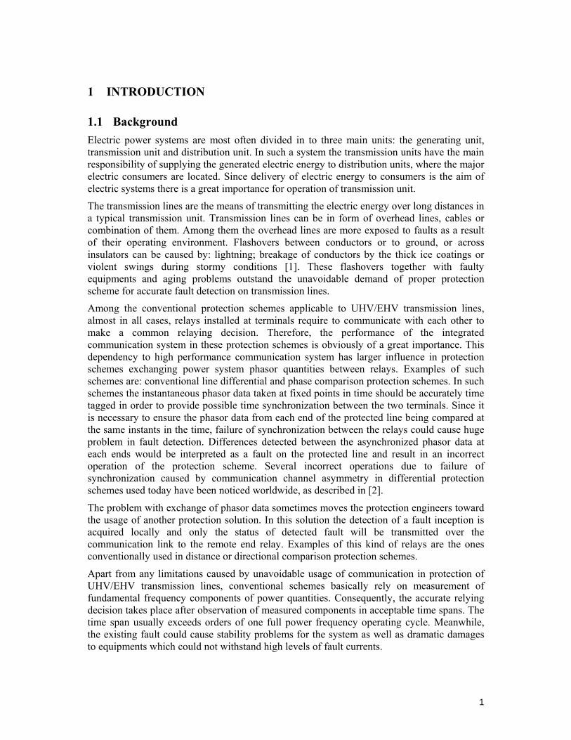
However, each disturbance in operation of one or more equipments can lead to abnormal system operating condition. These abnormal conditions may cause severe equipment damages. Therefore, to prevent severe damages and maintain the normal operating condition, monitoring of individual elements’ operation and development of protection schemes for entire system are of great importance. Usually different protection schemes with responsibility to protect the electrical equipments located in identified overlapping zones known as protection zones provide protection for an entire system, as shown in Figure 2.1.

Figure 2.1 Overlapping protection zones in a power system [6]

Such protection schemes shall pose the following characteristics [7]:

o Dependability: the protection scheme must be able to operate correctively when it is expected to operate. This is the degree of certainty that the scheme will operate correctly.

o Security: the protection scheme must be able to avoid unnecessary operation in non-fault conditions or inception of faults outside their protection zones. This is the degree of certainty that the scheme will not operate incorrectly.

o Sensitivity: the protection scheme must be able to detect the changes in the system in order to distinguish between normal and faulted operation of power system elements.

o Selectivity: the protection scheme must be able to correctly locate the inception of the fault and discriminate between the faults inside its protection zone and outside the protection zone.

o Fast operation: it is desirable that the protection scheme isolate the fault affected parts of the system as rapidly as possible in order to maintain stability of the overall power system and reduce damages to equipment and property.

4

The protection scheme contains measurement equipments, protection relays, circuit breakers, etc. The relays play the most important role in protection scheme because they detect the fault, determine fault location and also by closing trip coils send tripping command to circuit breakers. Design of such relays undertakes considerable technological developments from the first immerged relays and can be classified as [6]:

o Electromechanical relays - in the earliest design of protection relays moving mechanical parts were utilized. Working principal of electromechanical relays is based on the electromagnetic interactions. In these relays by inception of fault the current flow in one or more windings on a magnetic core or cores results in mechanical forces required to move the mechanical parts.

o Solid-state relays - these relays perform the same functions as electromagnetic relays

by use of analogue electronic devices instead of coils and magnets. Therefore, they can be considered as an analogue electronic replacement for electromechanical relays. The protection functions are acquired by an analogue process of measured signals. Electronic devices such as transistors and diodes in combination with resistors, capacitors, inductors, etc., enable the signal processing and implementation of protection algorithms in such relay design.

o Numerical relays – in numerical relays microprocessors are used for implementation

of the same protection logics as in case of the static relays. Processing of signals is carried out by conversion of input analogue signals into a digital representation and processing according to the appropriate protection algorithms implemented in the processors.

Nowadays, numerical relays utilizing digital techniques are used to protect almost all components of power systems. Furthermore a large number of functions previously implemented in separate protection relays can now be integrated in a single numerical relay unit.

2.2 Overview of transmission line protection schemes In protection of transmission lines the length of lines together with several factors related to the power system’s requirements and configurations affect the selection of a proper scheme. In IEEE for protection studies, in spite of using physical length of the line between both ends, a classification according to Source-to-line Impedance Ratios (SIRs) is given, [8], where:

o Transmission line with 4 SIR defined as short line, o Transmission line with 0.5 SIR 4 defined as medium line, o Transmission line with SIR 0.5 defined as long line.

Obviously, nominal operating voltage level of a line has a significant effect on the SIRs and therefore this classification will be assigned to different physical lengths in the following lines:

o High Voltage (HV) transmission lines with voltage levels of 69-230kV, o Extra High Voltage (EHV) transmission lines with voltage levels of 230-350kV, o Ultra High Voltage (UHV) transmission lines with voltage levels over 350kV.

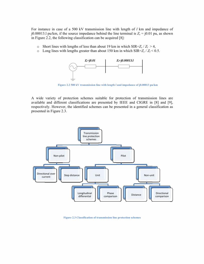
For instaj0.00013in Figure

o So L

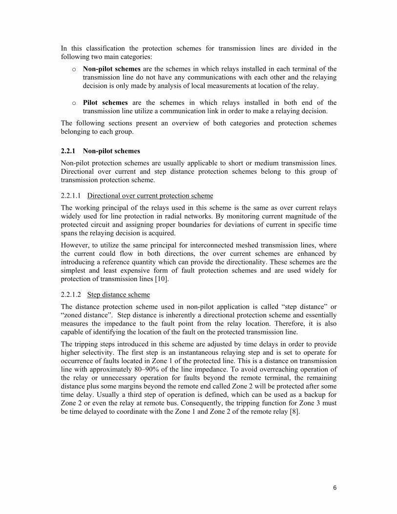
A wide availablerespectivpresented

Directicu

ance in case.l pu/km, if

e 2.2, the foll

hort lines wLong lines wi

Figu

variety of e and differevely. Howevd in Figure 2

Non‐pilo

onal over rrent

e of a 500 kthe source imlowing class

ith lengths oith lengths g

ure 2.2 500 kV t

protection ent classificer, the ident

2.3.

Figure 2.3 Cla

ot

Step distance

Lodi

kV transmissmpedance bsification can

of less than agreater than a

Zs=j0.01

transmission lin

schemes sucations are ptified schem

assification of tr

Transmissionline protection

schemes

Un

ngitudinal fferential

sion line wiehind the linn be acquired

about 19 kmabout 150 km

ne with length l

uitable for ppresented by

mes can be pr

ransmission line

n n 

it

Phase comparison

th length ofne terminal id [8]:

in which SIm in which S

Zl=j0.00013.l

l and impedance

protection oy IEEE andresented in a

e protection sch

Pilot

n Dis

f l km and iis Zs = j0.01

IR=Zs / Zl > SIR=Zs / Zl <

e of j0.00013 pu

of transmissd CIGRE ina general cla

hemes

Non‐un

stance

impedance opu, as show

4, < 0.5.

u/km

ion lines arn [8] and [9assification a

nit

Directional comparison

of wn

re 9], as

6

In this classification the protection schemes for transmission lines are divided in the following two main categories:

o Non-pilot schemes are the schemes in which relays installed in each terminal of the transmission line do not have any communications with each other and the relaying decision is only made by analysis of local measurements at location of the relay.

o Pilot schemes are the schemes in which relays installed in both end of the transmission line utilize a communication link in order to make a relaying decision.

The following sections present an overview of both categories and protection schemes belonging to each group.

2.2.1 Non-pilot schemes

Non-pilot protection schemes are usually applicable to short or medium transmission lines. Directional over current and step distance protection schemes belong to this group of transmission protection scheme.

2.2.1.1 Directional over current protection scheme

The working principal of the relays used in this scheme is the same as over current relays widely used for line protection in radial networks. By monitoring current magnitude of the protected circuit and assigning proper boundaries for deviations of current in specific time spans the relaying decision is acquired.

However, to utilize the same principal for interconnected meshed transmission lines, where the current could flow in both directions, the over current schemes are enhanced by introducing a reference quantity which can provide the directionality. These schemes are the simplest and least expensive form of fault protection schemes and are used widely for protection of transmission lines [10].

2.2.1.2 Step distance scheme

The distance protection scheme used in non-pilot application is called “step distance” or “zoned distance”. Step distance is inherently a directional protection scheme and essentially measures the impedance to the fault point from the relay location. Therefore, it is also capable of identifying the location of the fault on the protected transmission line.

The tripping steps introduced in this scheme are adjusted by time delays in order to provide higher selectivity. The first step is an instantaneous relaying step and is set to operate for occurrence of faults located in Zone 1 of the protected line. This is a distance on transmission line with approximately 80–90% of the line impedance. To avoid overreaching operation of the relay or unnecessary operation for faults beyond the remote terminal, the remaining distance plus some margins beyond the remote end called Zone 2 will be protected after some time delay. Usually a third step of operation is defined, which can be used as a backup for Zone 2 or even the relay at remote bus. Consequently, the tripping function for Zone 3 must be time delayed to coordinate with the Zone 1 and Zone 2 of the remote relay [8].

7

2.2.2 Pilot schemes

The non-pilot protection schemes discussed in previous section have usually an acceptable performance on short or medium lines. However, for long lines which are mostly operating in EHV or UHV levels and transmitting large electric power, the tripping time delays would cause severe network stability problems due to the system acceleration. Also the huge fault currents could cause dramatic damages for equipments. In such cases, more complex transmission line protection schemes are required in order to perform a high speed tripping in both ends of the line [10].

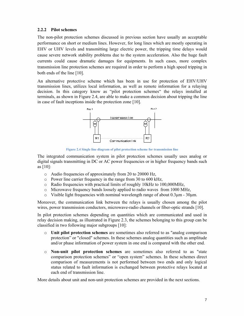
An alternative protective scheme which has been in use for protection of EHV/UHV transmission lines, utilizes local information, as well as remote information for a relaying decision. In this category know as “pilot protection schemes“ the relays installed at terminals, as shown in Figure 2.4, are able to make a common decision about tripping the line in case of fault inceptions inside the protection zone [10].

Figure 2.4 Single line diagram of pilot protection scheme for transmission line

The integrated communication system in pilot protection schemes usually uses analog or digital signals transmitting in DC or AC power frequencies or in higher frequency bands such as [10]:

o Audio frequencies of approximately from 20 to 20000 Hz, o Power line carrier frequency in the range from 30 to 600 kHz, o Radio frequencies with practical limits of roughly 10kHz to 100,000MHz, o Microwave frequency bands loosely applied to radio waves from 1000 MHz, o Visible light frequencies with nominal wavelength range of about 0.3μm - 30μm.

Moreover, the communication link between the relays is usually chosen among the pilot wires, power transmission conductors, microwave-radio channels or fiber-optic strands [10].

In pilot protection schemes depending on quantities which are communicated and used in relay decision making, as illustrated in Figure 2.3, the schemes belonging to this group can be classified in two following major subgroups [10]:

o Unit pilot protection schemes are sometimes also referred to as "analog comparison protection” or "closed" schemes. In these schemes analog quantities such as amplitude and/or phase information of power system in one end is compared with the other end.

o Non-unit pilot protection schemes are sometimes also referred to as "state comparison protection schemes” or “open system” schemes. In these schemes direct comparison of measurements is not performed between two ends and only logical status related to fault information is exchanged between protective relays located at each end of transmission line.

More details about unit and non-unit protection schemes are provided in the next sections.

8

2.2.2.1 Unit Protection Schemes

Two important unit pilot protection schemes are identified as longitudinal differential and phase comparison schemes. In such schemes the main communicated information between the ends of the protected line are either amplitude and/or phase data of the transmission line components.

In case of an internal fault the result of the compared data will be a differential value and for specific threshold values the relays in both terminals perform a relaying operation. Since there is an instantaneous comparison between the analog values, the information acquired from both relays needs to be time synchronized to guarantee the comparison of measured data at same time instants from both ends [10]. Longitudinal Differential Scheme

Longitudinal pilot systems are based on basic principle scheme proposed by Charles H. Merz and Bernard Price in 1904. The operation principle of the relay is expressed by Kirchhoff’s first law that says: “the sum of the currents flowing to a node must be equal with the sum of the currents leaving the same node” [1].

In external faults the same current is entering to protected zone and leaving it from the second end. But in case of internal fault the current entering the protected zone is not equal to the current which is leaving the same zone. Therefore, this principal could be utilized in directional protection schemes for protection of transmission lines. Phase Comparison Scheme

In a phase comparison scheme the relay is able to distinguish an internal inception of the fault on protected transmission line by comparing the current phase angle at one end with current phase angle at the second end. Where in case of the internal faults there will be a notable phase difference [10]. However, incorrect operation of the relay can happen by changing the system configuration which may affect the polarity of the quantities used for directional comparison [12].

2.2.2.2 Non-unit Protection Schemes

Two important non-unit pilot protection schemes are identified as distance and directional comparison schemes. In such schemes the logical information typically related to direction of the fault are sent over the communication link for a common relaying decision. Therefore, there will be less dependency on data synchronization comparing to unit protection schemes [11]. Distance Scheme

Communication link between relays in pilot distance schemes can eliminate the time delays for relay decision makings in case of occurrence of faults in second or even third zones for distance protection schemes. Thus, the local relays can communicate with the remote relay in order to make sure that the detected fault is located on protected zone. This provides fast directional fault detection as well as opportunity of implementing the step distance relays in protection of long transmission lines [10].

9

Directional Comparison Scheme

The relays in directional comparison pilot schemes, such as directional over current relays, detect the direction to the fault at their local position and share the information with the remote terminal relay. Consequently, the overall functionality of the scheme can be accomplished by a common decision from both ends. Furthermore, the new generation of transmission line protection schemes called Ultra-High-Speed relaying (UHS) schemes, which is the subject of this study, belongs also to this group.

Excluding UHS relaying schemes, almost in all the protection schemes introduced in this chapter, the schemes are based on the observation of the fundamental frequency components and an accurate decision making about the faults taking place in time spans equal or longer than one full power frequency operating cycle (in case of systems operating at 50Hz frequency this time exceeds 20 ms) [1].

Protection schemes based on fundamental frequency components usually are referred as ‘conventional’ or ‘classical’ transmission protection schemes. In these schemes both high and low frequency components in current and voltage quantities introduced by any disturbances in the power system are considered as noise to main signals and are used to be filtered out in order to perform the analysis [10,13]. However, in the early 1970s, it has been discovered that according to concept of traveling waves (as described in the next chapter), transient analysis of power system’s quantities at inception of the faults provide new possibility of fault detections. These transients contain extensive information about the fault and can be used in UHS protection schemes with ability of [13]:

o Fault direction determination, o Fault type discrimination, o Fault location identification.

10

3 TRAVELING WAVES ON TRANSMISSION LINES

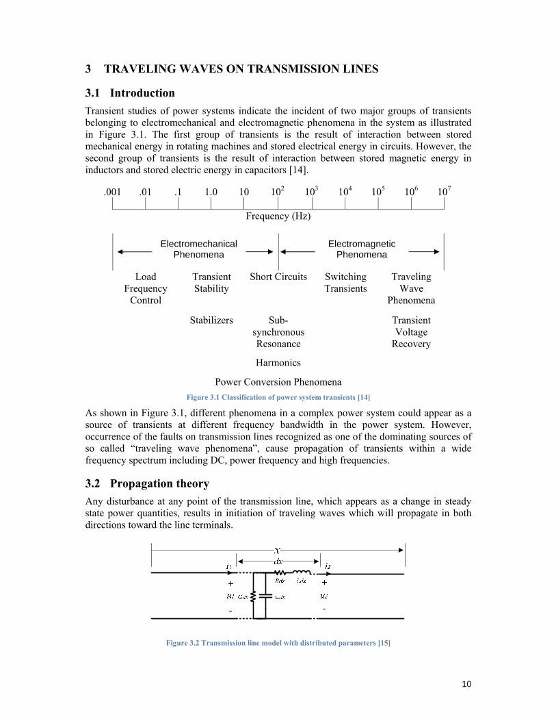
3.1 Introduction Transient studies of power systems indicate the incident of two major groups of transients belonging to electromechanical and electromagnetic phenomena in the system as illustrated in Figure 3.1. The first group of transients is the result of interaction between stored mechanical energy in rotating machines and stored electrical energy in circuits. However, the second group of transients is the result of interaction between stored magnetic energy in inductors and stored electric energy in capacitors [14].

.001 .01 .1 1.0 10 102 103 104 105 106 107

Frequency (Hz)

Load Frequency

Control

Transient Stability

Short Circuits Switching Transients

Traveling Wave

Phenomena

Stabilizers Sub-synchronous Resonance

Transient Voltage

Recovery

Harmonics

Power Conversion Phenomena Figure 3.1 Classification of power system transients [14]

As shown in Figure 3.1, different phenomena in a complex power system could appear as a source of transients at different frequency bandwidth in the power system. However, occurrence of the faults on transmission lines recognized as one of the dominating sources of so called “traveling wave phenomena”, cause propagation of transients within a wide frequency spectrum including DC, power frequency and high frequencies.

3.2 Propagation theory Any disturbance at any point of the transmission line, which appears as a change in steady state power quantities, results in initiation of traveling waves which will propagate in both directions toward the line terminals.

Figure 3.2 Transmission line model with distributed parameters [15]

Electromechanical Phenomena

Electromagnetic Phenomena

11

Let us consider a small section of length dx of a transmission line with distributed parameters as shown in Figure 3.2. The voltage u and current i caused by some disturbance on transmission line would have the following total changes per unit length of the transmission line in the forward x direction [15].

(1)

(2)

Where

R is the resistance per unit length of the transmission line; L is the inductance per unit length of the transmission line; G is the conductance per unit length of the transmission line; C is the capacitance per unit length of the transmission line; ω is the angular frequency;

Cancelling dx from both sides of equations (1) and (2) can be written as:

(3)

(4)

In witch Z R jωL and Y G jωC are the impedance and admittance per unit length of the line, respectively.

Differentiating the coupled partial first order differential equations (3) and (4), which are the well-known differential equations of the single circuit transmission line, yield the following decoupled second order differential equations:

(5)

(6)

By solving equation (5) for u and calculating i from (3), the results can be written as:

(7)

(8)

By introducing and as arbitrary functions of time t, equation (7) and (8) are the general solution in terms of frequency dependent operator γ which is known as propagation constant and characterizes the propagation of voltage through the transmission line.

In equation (8), is called surge admittance of the line and its inverse function which has impedance dimension, is know as surge or characteristic impedance of the transmission line and is indicated by .

12

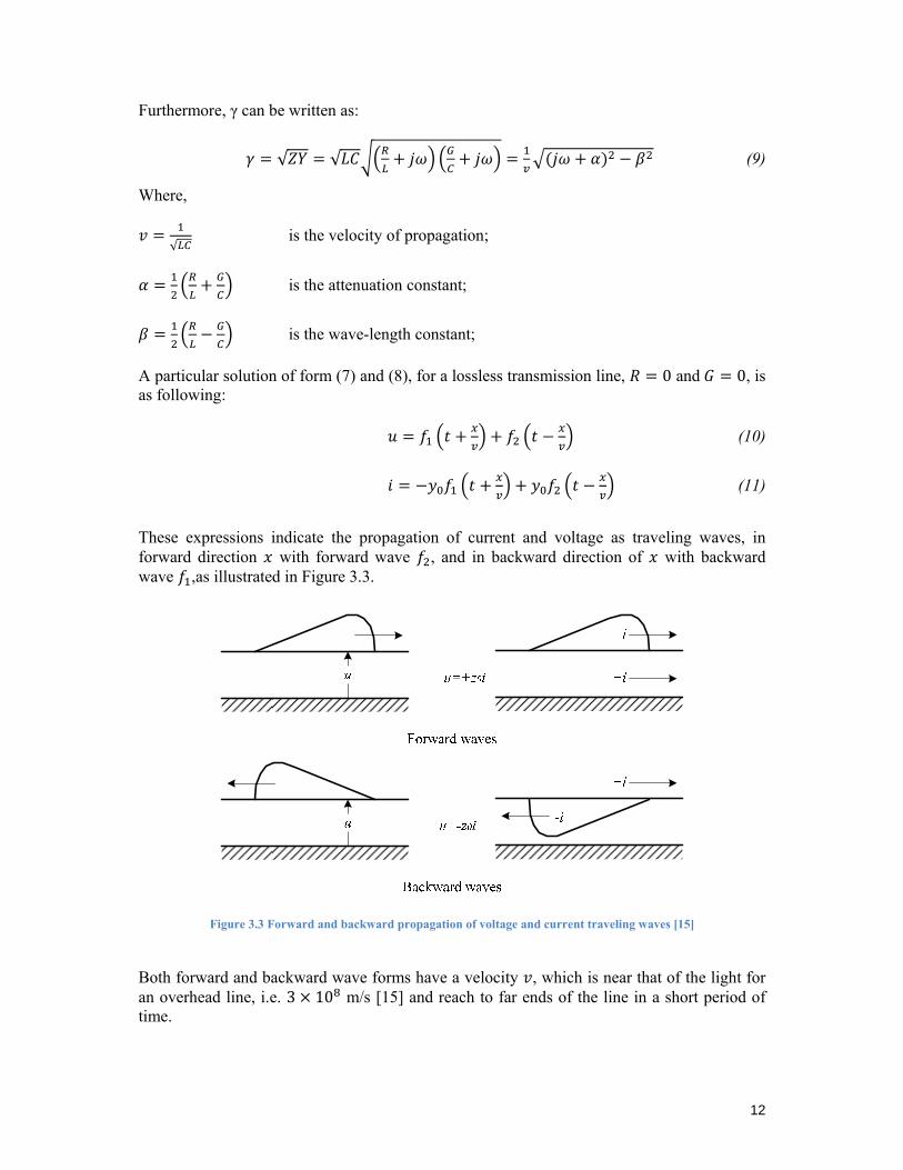
Furthermore, γ can be written as:

√ √ (9)

Where,

√ is the velocity of propagation;

is the attenuation constant;

is the wave-length constant;

A particular solution of form (7) and (8), for a lossless transmission line, 0 and 0, is as following:

(10)

(11)

These expressions indicate the propagation of current and voltage as traveling waves, in forward direction with forward wave , and in backward direction of with backward wave ,as illustrated in Figure 3.3.

Figure 3.3 Forward and backward propagation of voltage and current traveling waves [15]

Both forward and backward wave forms have a velocity , which is near that of the light for an overhead line, i.e. 3 10 m/s [15] and reach to far ends of the line in a short period of time.

13

As discussed before, the voltage and current traveling waves are related to each other through the characteristic impedance of the line such that and they appear as sudden deviations in measured voltage and current quantities from their pre-fault values with different polarities. These sudden deviations in voltage and current can be explained by application of superposition theorem for wave forms. This theorem is usually used to explain the phenomena of wave interference of both voltage waveforms and current waveforms propagating in power systems from different sources.

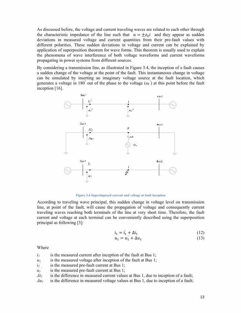
By considering a transmission line, as illustrated in Figure 3.4, the inception of a fault causes a sudden change of the voltage at the point of the fault. This instantaneous change in voltage can be simulated by inserting an imaginary voltage source at the fault location, which generates a voltage in 180° out of the phase to the voltage (uF

’) at this point before the fault inception [16].

Figure 3.4 Superimposed current and voltage at fault inception

According to traveling wave principal, this sudden change in voltage level on transmission line, at point of the fault, will cause the propagation of voltage and consequently current traveling waves reaching both terminals of the line at very short time. Therefore, the fault current and voltage at each terminal can be conveniently described using the superposition principal as following [3]:

i i′ ∆i (12) ′ ∆ (13)

Where

i1 is the measured current after inception of the fault at Bus 1; u1 is the measured voltage after inception of the fault at Bus 1; i1

’ is the measured pre-fault current at Bus 1; u1

’ is the measured pre-fault current at Bus 1; Δi1 is the difference in measured current values at Bus 1, due to inception of a fault; Δu1 is the difference in measured voltage values at Bus 1, due to inception of a fault;

14

By formulating the similar equations for the fault current and voltage at the second end of the line at Bus 2, it can be seen that the sudden deviation in voltage and current at Bus 1 and Bus 2 can be interpreted as an interference of traveling waves arrived to transmission line terminals with pre-fault voltage and current waveforms at the same location. Furthermore, due to reflection and refraction of traveling waves, as described in the following section, continuous variations known as traveling waves’ transients appear in measured voltage and current signals.

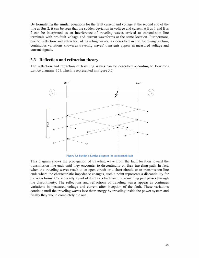
3.3 Reflection and refraction theory The reflection and refraction of traveling waves can be described according to Bewley’s Lattice diagram [15], which is represented in Figure 3.5.

Figure 3.5 Bewley’s Lattice diagram for an internal fault

This diagram shows the propagation of traveling wave from the fault location toward the transmission line ends until they encounter to discontinuity on their traveling path. In fact, when the traveling waves reach to an open circuit or a short circuit, or to transmission line ends where the characteristic impedance changes, such a point represents a discontinuity for the waveforms. Consequently a part of it reflects back and the remaining part passes through the discontinuity. The reflections and refractions of traveling waves appear as continues variations in measured voltage and current after inception of the fault. These variations continue until the traveling waves lose their energy by traveling inside the power system and finally they would completely die out.

15

3.4 Fault detection applications

UHS relay developed by ASEA

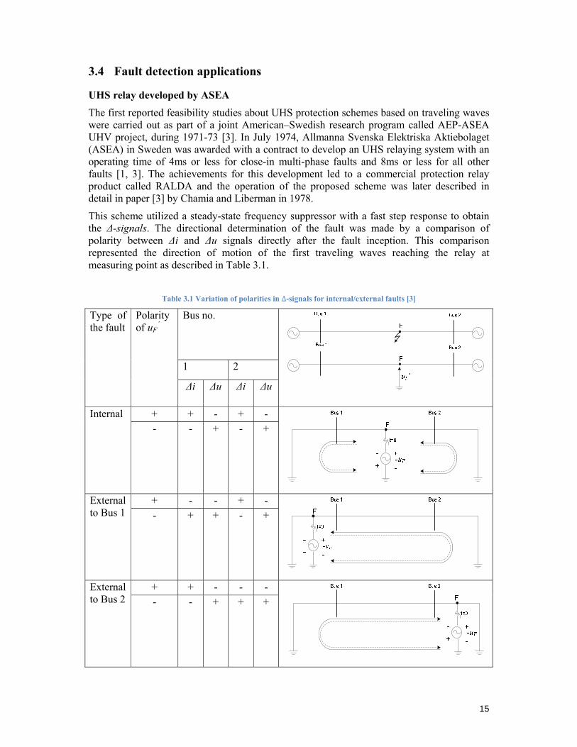
The first reported feasibility studies about UHS protection schemes based on traveling waves were carried out as part of a joint American–Swedish research program called AEP-ASEA UHV project, during 1971-73 [3]. In July 1974, Allmanna Svenska Elektriska Aktiebolaget (ASEA) in Sweden was awarded with a contract to develop an UHS relaying system with an operating time of 4ms or less for close-in multi-phase faults and 8ms or less for all other faults [1, 3]. The achievements for this development led to a commercial protection relay product called RALDA and the operation of the proposed scheme was later described in detail in paper [3] by Chamia and Liberman in 1978.

This scheme utilized a steady-state frequency suppressor with a fast step response to obtain the Δ-signals. The directional determination of the fault was made by a comparison of polarity between Δi and Δu signals directly after the fault inception. This comparison represented the direction of motion of the first traveling waves reaching the relay at measuring point as described in Table 3.1.

Table 3.1 Variation of polarities in ∆-signals for internal/external faults [3]

Type of the fault

Polarity of uF

’ Bus no.

1 2

Δi Δu Δi Δu

Internal + + - + - - - + - +

External to Bus 1

+ - - + - - + + - +

External to Bus 2

+ + - - - - - + + +

16

As shown in Table 3.1, the positive current sign is assumed in direction from the terminals toward the transmission line. The initial deviations (referred as Δ-signals) on each bus have opposite or same polarity for internal or external faults, respectively. Therefore, the decision about faults in short fraction of time (up to one power frequency cycle) is acquired by means of a communication link between relays located at Bus 1 and Bus 2 [3, 17, 18].

UHS relay developed by BBC

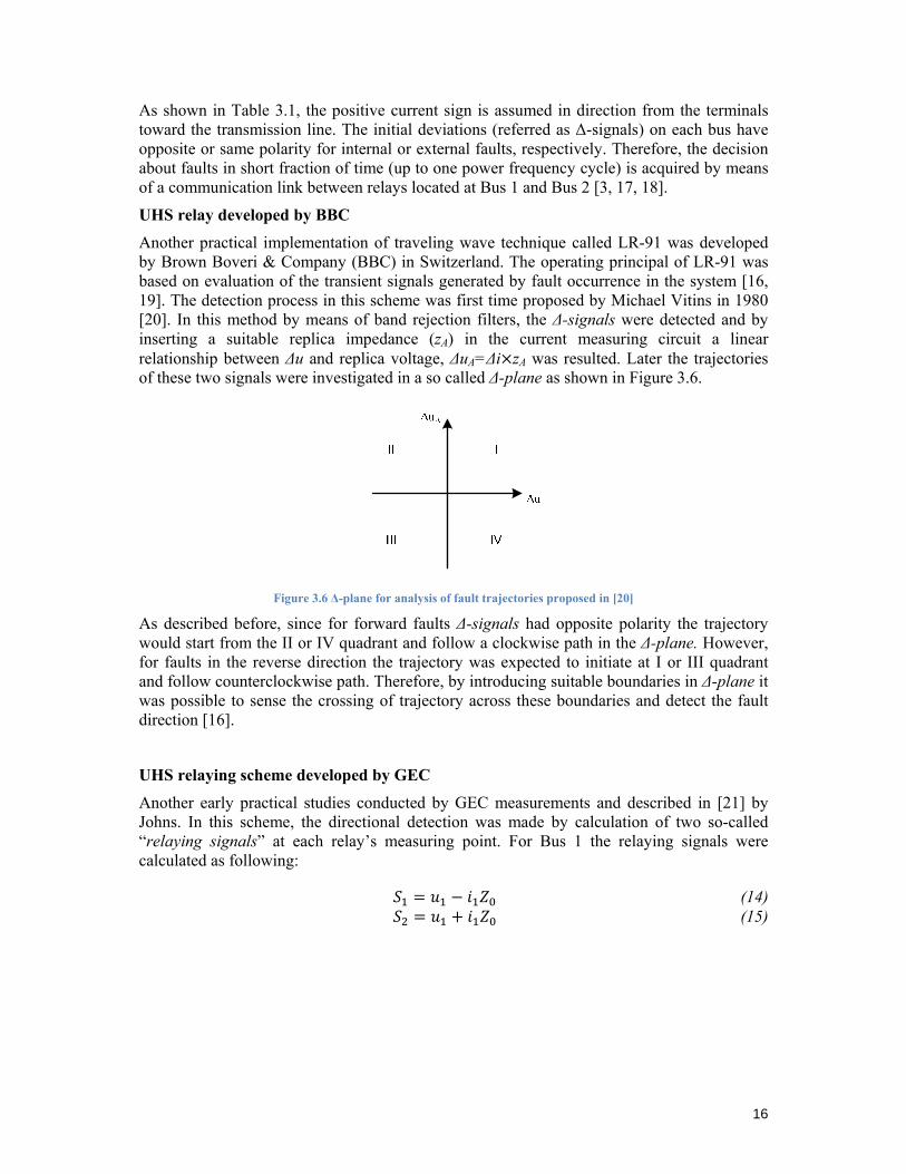
Another practical implementation of traveling wave technique called LR-91 was developed by Brown Boveri & Company (BBC) in Switzerland. The operating principal of LR-91 was based on evaluation of the transient signals generated by fault occurrence in the system [16, 19]. The detection process in this scheme was first time proposed by Michael Vitins in 1980 [20]. In this method by means of band rejection filters, the Δ-signals were detected and by inserting a suitable replica impedance (zA) in the current measuring circuit a linear relationship between Δu and replica voltage, ΔuA=Δi zA was resulted. Later the trajectories of these two signals were investigated in a so called Δ-plane as shown in Figure 3.6.

Figure 3.6 Δ-plane for analysis of fault trajectories proposed in [20]

As described before, since for forward faults Δ-signals had opposite polarity the trajectory would start from the II or IV quadrant and follow a clockwise path in the Δ-plane. However, for faults in the reverse direction the trajectory was expected to initiate at I or III quadrant and follow counterclockwise path. Therefore, by introducing suitable boundaries in Δ-plane it was possible to sense the crossing of trajectory across these boundaries and detect the fault direction [16].

UHS relaying scheme developed by GEC

Another early practical studies conducted by GEC measurements and described in [21] by Johns. In this scheme, the directional detection was made by calculation of two so-called “relaying signals” at each relay’s measuring point. For Bus 1 the relaying signals were calculated as following:

(14) (15)

17

Where

u1 is the superimposed voltage component measured at Bus 1; i1 is the superimposed current component measured at Bus 1; Z0 is the characteristics surge impedance of the transmission line; S1,S2 are the relaying signals;

According to polarity analysis of the incremental voltage and current at fault inception, calculation of two relaying signals during the reflection of traveling waves provided different increasing magnitude between the two signals. Then by monitoring of the increasing levels of these signals the discrimination between internal and external faults were accomplished [21].

Furthermore, according to reflection and refraction properties of the traveling waves protection schemes for determination of faults’ position on transmission lines were also proposed [22]. However, such schemes required directional detection technique and a method to discriminate between the reflected waves from the fault point and the other traveling waves arriving at measuring point. Afterwards, by intelligent time tagging of desired reflections of the waves, an accurate determination of fault location could be conducted.

3.4.1 Technical obstacles for early developed schemes

The fast response of these early developed protection schemes introduced new transmission line protection approach for the continuously expanding power systems with a demand for fast fault clearance. However, the fast operation of these relays was usually affected by long time delay introduced by operation of circuit breakers and communication networks. Furthermore, the implementation of such methods in a numerical relay at that time required the fast data processors to reach the ultra high speed relaying response. However, those sorts of processors were not available with as advanced technology and low price as today. Thus, the requirements for fast operation of auxiliary devices needed in overall protection scheme increased the development costs and created obstacles for the new approach to become a major protection solution.

3.4.2 Existing solutions for developing new schemes

Recently the interest for developing UHS numerical relay has increased due to successful performance of numerical relays in conventional protection schemes, availability of fast digital data processors with lower prices and significant technology improvements in design of electronic equipments and communication systems.

Literature reviews carried out for this thesis indicate that there are plenty of publications about development of new UHS numerical relays utilizing the traveling wave concepts. They are usually referred as Traveling Wave Relays. The recently proposed solutions provide ability of detecting and locating the faults on transmission lines based on the analysis of traveling waves’ transients in wide range of frequencies. However, new studies often contribute to earlier achievements, but they have complexities and special requirements for practical implementation and may not lead to commercial production. Investigations about practical issues leading to these complexities are presented in the next chapter.

18

4 STUDY OF PRACTICAL ISSUES FOR DEVELOPMENT OF TRAVELING WAVE RELAYS

4.1 Introduction This chapter presents the studies carried out in order to identify the main issues with analysis of traveling waves in wide frequency bandwidth in traveling wave based protection methods.

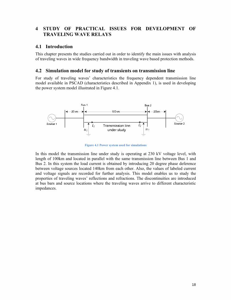
4.2 Simulation model for study of transients on transmission line For study of traveling waves’ characteristics the frequency dependent transmission line model available in PSCAD (characteristics described in Appendix 1), is used in developing the power system model illustrated in Figure 4.1.

Figure 4.1 Power system used for simulations

In this model the transmission line under study is operating at 230 kV voltage level, with length of 100km and located in parallel with the same transmission line between Bus 1 and Bus 2. In this system the load current is obtained by introducing 20 degree phase deference between voltage sources located 140km from each other. Also, the values of labeled current and voltage signals are recorded for further analysis. This model enables us to study the properties of traveling waves’ reflections and refractions. The discontinuities are introduced at bus bars and source locations where the traveling waves arrive to different characteristic impedances.

19

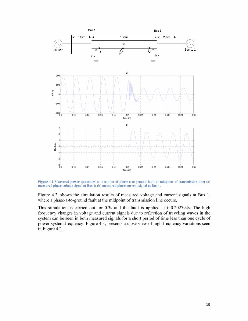
Figure 4.2 Measured power quantities at inception of phase-a-to-ground fault at midpoint of transmission line; (a) measured phase voltage signal at Bus 1; (b) measured phase current signal at Bus 1.

Figure 4.2, shows the simulation results of measured voltage and current signals at Bus 1, where a phase-a-to-ground fault at the midpoint of transmission line occurs.

This simulation is carried out for 0.3s and the fault is applied at t=0.202794s. The high frequency changes in voltage and current signals due to reflection of traveling waves in the system can be seen in both measured signals for a short period of time less than one cycle of power system frequency. Figure 4.3, presents a close view of high frequency variations seen in Figure 4.2.

0.1 0.12 0.14 0.16 0.18 0.2 0.22 0.24 0.26 0.28 0.3-200

-100

0

100

200

Time (s)

U1a

(kV

)

(a)

0.1 0.12 0.14 0.16 0.18 0.2 0.22 0.24 0.26 0.28 0.3-3

-2

-1

0

1

2

3

Time (s)

I1a

(kA

)

(b)

20

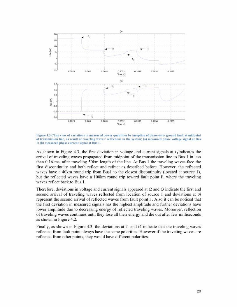
Figure 4.3 Close view of variations in measured power quantities by inception of phase-a-to- ground fault at midpoint of transmission line, as result of traveling waves’ reflections in the system; (a) measured phase voltage signal at Bus 1; (b) measured phase current signal at Bus 1.

As shown in Figure 4.3, the first deviation in voltage and current signals at indicates the arrival of traveling waves propagated from midpoint of the transmission line to Bus 1 in less than 0.16 ms, after traveling 50km length of the line. At Bus 1 the traveling waves face the first discontinuity and both reflect and refract as described before. However, the refracted waves have a 40km round trip from Bus1 to the closest discontinuity (located at source 1), but the reflected waves have a 100km round trip toward fault point F, where the traveling waves reflect back to Bus 1.

Therefore, deviations in voltage and current signals appeared at t2 and t3 indicate the first and second arrival of traveling waves reflected from location of source 1 and deviations at t4 represent the second arrival of reflected waves from fault point F. Also it can be noticed that the first deviation in measured signals has the highest amplitude and further deviations have lower amplitude due to decreasing energy of reflected traveling waves. Moreover, reflection of traveling waves continues until they lose all their energy and die out after few milliseconds as shown in Figure 4.2.

Finally, as shown in Figure 4.3, the deviations at t1 and t4 indicate that the traveling waves reflected from fault point always have the same polarities. However if the traveling waves are reflected from other points, they would have different polarities.

0.2029 0.203 0.2031 0.2032 0.2033 0.2034 0.2035-100

-50

0

50

100

150

200

Time (s)

U1a

(kV

)

(a)

0.2029 0.203 0.2031 0.2032 0.2033 0.2034 0.2035

-0.3

-0.2

-0.1

0

0.1

0.2

0.3

Time (s)

I1a

(kA

)

(b)

t1

t2

t3

t4

t1

t2

t3

t4

21

4.3 Recognized practical implementation issues

4.3.1 Signal-to-noise ratio

Moving from analog to digital technology in development of numerical relays in the recent proposals requires mapping of continuous data sequence in analog signals to desecrated data. These data are samples taken from the original analog signals in specific time intervals. Therefore, the highest frequency component appearing in digital signal is a finite frequency referred to as Nyquist frequency and is highly dependent on the sampling rate (or sampling frequency).

In digital signal processing the non-bounded frequency analog signal shall be limited to a bounded frequency signal before conversion to digital signal. This requirement is needed to avoid a conversion which aliases another signal rather than the original analog signal (for much higher rate of changes in analog signal than the sampling rate). Thus, the frequencies outside the Nyquist bandwidth shall be rejected before the sampling process.

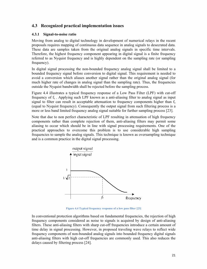
Figure 4.4 illustrates a typical frequency response of a Low Pass Filter (LPF) with cut-off frequency of fc . Applying such LPF known as a anti-aliasing filter to analog signal as input signal to filter can result in acceptable attenuation to frequency components higher than fc (equal to Nyquist frequency). Consequently the output signal from such filtering process is a more or less band limited frequency analog signal suitable for further sampling process [23].

Note that due to non perfect characteristic of LPF resulting in attenuation of high frequency components rather than complete rejection of them, anti-aliasing filters may permit some aliasing to occur which should be in line with signal processing requirements. One of the practical approaches to overcome this problem is to use considerable high sampling frequencies to sample the analog signals. This technique is known as oversampling technique and is a common practice in the digital signal processing.

2/1

Figure 4.4 Typical frequency response of a low pass filter [23]

In conventional protection algorithms based on fundamental frequencies, the rejection of high frequency components considered as noise to signals is acquired by design of anti-aliasing filters. These anti-aliasing filters with sharp cut-off frequencies introduce a certain amount of time delay in signal processing. However, in proposed traveling wave relays to reflect wide frequency components of non-bounded analog signals into bounded frequency digital signals anti-aliasing filters with high cut-off frequencies are commonly used. This also reduces the delays caused by filtering process [24].

22

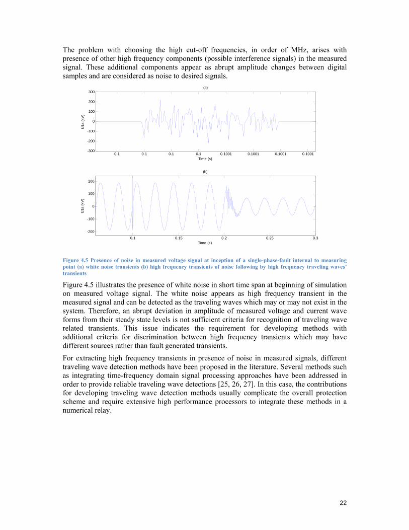
The problem with choosing the high cut-off frequencies, in order of MHz, arises with presence of other high frequency components (possible interference signals) in the measured signal. These additional components appear as abrupt amplitude changes between digital samples and are considered as noise to desired signals.

Figure 4.5 Presence of noise in measured voltage signal at inception of a single-phase-fault internal to measuring point (a) white noise transients (b) high frequency transients of noise following by high frequency traveling waves’ transients

Figure 4.5 illustrates the presence of white noise in short time span at beginning of simulation on measured voltage signal. The white noise appears as high frequency transient in the measured signal and can be detected as the traveling waves which may or may not exist in the system. Therefore, an abrupt deviation in amplitude of measured voltage and current wave forms from their steady state levels is not sufficient criteria for recognition of traveling wave related transients. This issue indicates the requirement for developing methods with additional criteria for discrimination between high frequency transients which may have different sources rather than fault generated transients.

For extracting high frequency transients in presence of noise in measured signals, different traveling wave detection methods have been proposed in the literature. Several methods such as integrating time-frequency domain signal processing approaches have been addressed in order to provide reliable traveling wave detections [25, 26, 27]. In this case, the contributions for developing traveling wave detection methods usually complicate the overall protection scheme and require extensive high performance processors to integrate these methods in a numerical relay.

0.1 0.1 0.1 0.1 0.1001 0.1001 0.1001 0.1001-300

-200

-100

0

100

200

300

Time (s)

U1a

(kV

)(a)

0.1 0.15 0.2 0.25 0.3

-200

-100

0

100

200

Time (s)

U1a

(kV

)

(b)

23

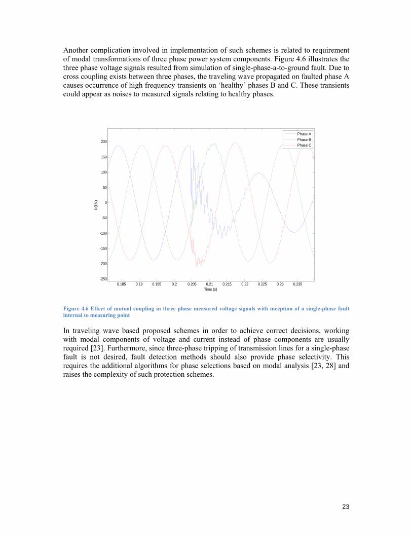
Another complication involved in implementation of such schemes is related to requirement of modal transformations of three phase power system components. Figure 4.6 illustrates the three phase voltage signals resulted from simulation of single-phase-a-to-ground fault. Due to cross coupling exists between three phases, the traveling wave propagated on faulted phase A causes occurrence of high frequency transients on ‘healthy’ phases B and C. These transients could appear as noises to measured signals relating to healthy phases.

Figure 4.6 Effect of mutual coupling in three phase measured voltage signals with inception of a single-phase fault internal to measuring point

In traveling wave based proposed schemes in order to achieve correct decisions, working with modal components of voltage and current instead of phase components are usually required [23]. Furthermore, since three-phase tripping of transmission lines for a single-phase fault is not desired, fault detection methods should also provide phase selectivity. This requires the additional algorithms for phase selections based on modal analysis [23, 28] and raises the complexity of such protection schemes.

0.185 0.19 0.195 0.2 0.205 0.21 0.215 0.22 0.225 0.23 0.235-250

-200

-150

-100

-50

0

50

100

150

200

Time (s)

U(k

V)

Phase APhase BPhase C

24

4.3.2 Frequency responses of measuring equipments

The traveling wave based protection algorithms are usually based on analysis of measured transients in voltage and current quantities at transmission line terminals. The traveling waves propagated in the system due to fault inceptions result in a dominant change in a wide frequency spectrum of the measured quantities. Any attenuation or delay in measuring of these frequency components in voltage and/or current quantities is considered as loss of information and could influence the performance of the relay. However, measuring equipments with energy storage components such as capacitances and inductances can not provide desirable frequency responses for immediate changes in measured quantities. In this case measuring equipment acts as a filter for high frequency components available in the original signal and consequently causes distortions of desired transients in the measured signal.

In high voltage transmission lines usually Current Transformers (CTs) and Coupled Capacitor Voltage Transformers (CCVTs) are used for measuring current and voltage, respectively. The problems can usually arise due to limited frequency band response of the widely used CCVTs consist of capacitive voltage divider in series with a magnetic Voltage Transformer (VT). CCVTs are usually tuned to have linear responses for specific bandwidth of frequencies up to a few kHz in order to provide reliable voltage measurements in fundamental power system frequencies and their behavior is not known for other ranges. In [29] more details about tuning factors in the design of CCVTs and the corresponding frequency responses can be found.

To study this limiting factor three different simulations applying CT and CCVT models available in PSCAD library (presented in Appendix 2) and four ABB measurement instrument models (CPB 245, IMB 245, CPA 245 and IMBD 245) with different tuned frequency responses used in practice for measurement of voltages and currents are carried out. The obtained results are compared and presented below.

25

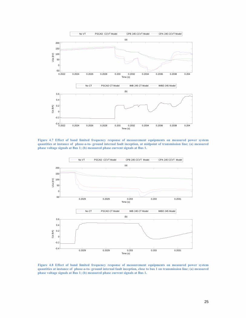
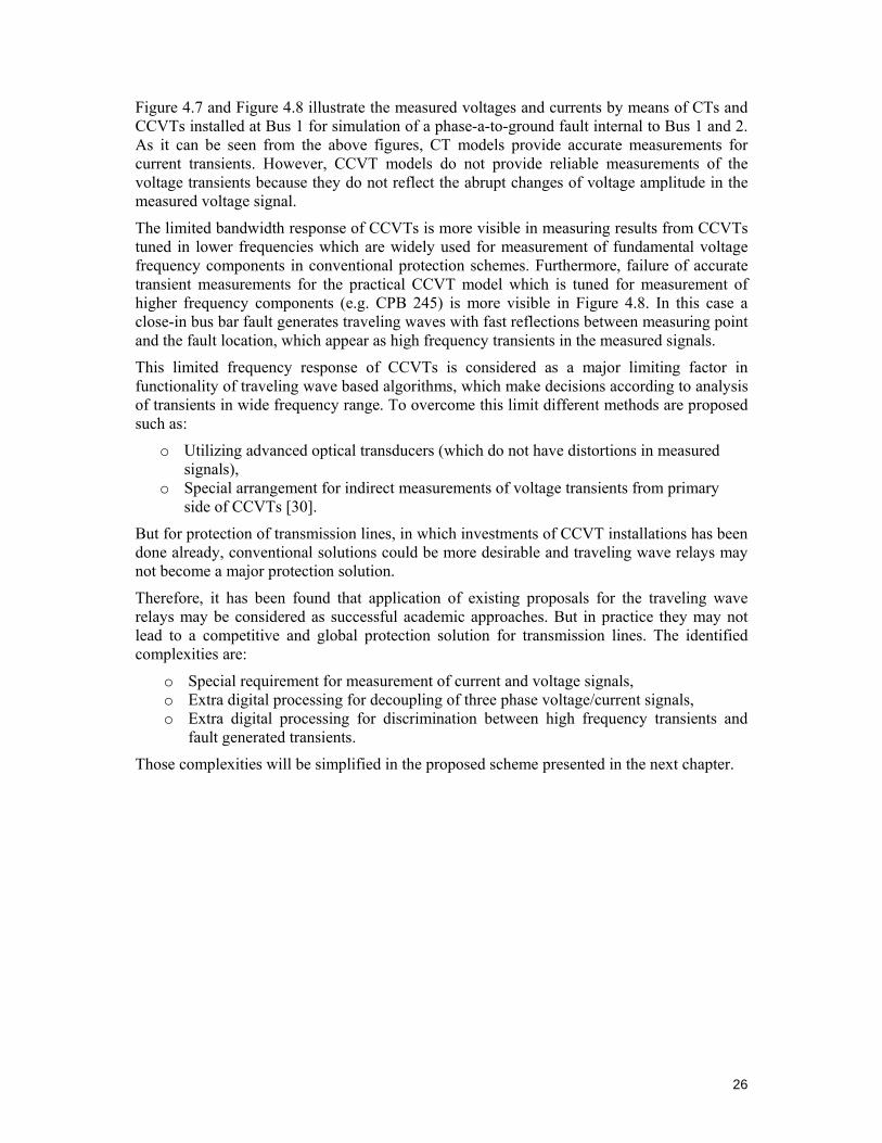
Figure 4.7 Effect of band limited frequency response of measurement equipments on measured power system quantities at instance of phase-a-to- ground internal fault inception, at midpoint of transmission line; (a) measured phase voltage signals at Bus 1; (b) measured phase current signals at Bus 1.

Figure 4.8 Effect of band limited frequency response of measurement equipments on measured power system quantities at instance of phase-a-to- ground internal fault inception, close to bus 1 on transmission line; (a) measured phase voltage signals at Bus 1; (b) measured phase current signals at Bus 1.

0.2022 0.2024 0.2026 0.2028 0.203 0.2032 0.2034 0.2036 0.2038 0.204-50

0

50

100

150

200

Time (s)

U1a

(kV

)

(a)

0.2022 0.2024 0.2026 0.2028 0.203 0.2032 0.2034 0.2036 0.2038 0.204-0.4

-0.2

0

0.2

0.4

0.6

Time (s)

I1a

(kA

)

(b)

No VT PSCAD CCVT Model CPB 245 CCVT Model CPA 245 CCVT Model

No CT PSCAD CT Model IMB 245 CT Model IMBD 245 Model

0.2029 0.2029 0.203 0.203 0.2031-50

0

50

100

150

200

Time (s)

U1a

(kV

)

(a)

0.2029 0.2029 0.203 0.203 0.2031-0.4

-0.2

0

0.2

0.4

0.6

Time (s)

I1a

(kA

)

(b)

No VT PSCAD CCVT Model CPB 245 CCVT Model CPA 245 CCVT Model

No CT PSCAD CT Model IMB 245 CT Model IMBD 245 Model

26

Figure 4.7 and Figure 4.8 illustrate the measured voltages and currents by means of CTs and CCVTs installed at Bus 1 for simulation of a phase-a-to-ground fault internal to Bus 1 and 2. As it can be seen from the above figures, CT models provide accurate measurements for current transients. However, CCVT models do not provide reliable measurements of the voltage transients because they do not reflect the abrupt changes of voltage amplitude in the measured voltage signal.

The limited bandwidth response of CCVTs is more visible in measuring results from CCVTs tuned in lower frequencies which are widely used for measurement of fundamental voltage frequency components in conventional protection schemes. Furthermore, failure of accurate transient measurements for the practical CCVT model which is tuned for measurement of higher frequency components (e.g. CPB 245) is more visible in Figure 4.8. In this case a close-in bus bar fault generates traveling waves with fast reflections between measuring point and the fault location, which appear as high frequency transients in the measured signals.

This limited frequency response of CCVTs is considered as a major limiting factor in functionality of traveling wave based algorithms, which make decisions according to analysis of transients in wide frequency range. To overcome this limit different methods are proposed such as:

o Utilizing advanced optical transducers (which do not have distortions in measured signals),

o Special arrangement for indirect measurements of voltage transients from primary side of CCVTs [30].

But for protection of transmission lines, in which investments of CCVT installations has been done already, conventional solutions could be more desirable and traveling wave relays may not become a major protection solution.

Therefore, it has been found that application of existing proposals for the traveling wave relays may be considered as successful academic approaches. But in practice they may not lead to a competitive and global protection solution for transmission lines. The identified complexities are:

o Special requirement for measurement of current and voltage signals, o Extra digital processing for decoupling of three phase voltage/current signals, o Extra digital processing for discrimination between high frequency transients and

fault generated transients.

Those complexities will be simplified in the proposed scheme presented in the next chapter.

27

5 PROPOSED RELAYING SOLUTION

5.1 Introduction According to studies presented in previous chapter it has been noticed that development of new schemes for extracting traveling wave related data has been imposed by practical limitations. As a result of increasing demand for development of numerical protection relays with UHS feature and difficulties with development of traveling wave based schemes a series of new research has been carried out. New studies are focusing on utilizing limited bandwidth of frequencies for analysis of transients measured in voltage and/or current signals at inception of faults and are referred as Transient Based Fault Detection approach [31].

In this technique the bandwidth of measured quantities is limited to a few kHz where even limitation of frequency response of conventional transformers, as well as, high frequency interferences in measured quantities could be eliminated. It is checked if the initial deviation in measured voltage and current signals in bounded frequencies posses the same polarities as in non-bounded frequency signals.

In this chapter before conversion of analogue signals to bounded frequency digital signals, first the effect of fault nature in characteristics and behavior of traveling waves is presented. Later by introducing the requirements to limit the frequency components in measured signals the proposed directional comparison pilot protection scheme is presented.

5.2 Study of behavior and characteristics of traveling waves in different fault conditions

The protection scheme based on the traveling wave principal for detecting the faults on 100% length of the transmission lines should not be affected by different fault cases. However, characteristics of transients caused by traveling waves are directly related to nature of a fault which can be a function of several variables such as:

o Type of the fault, o Resistances of the fault (in case of phase to ground faults), o Inception angle of the fault, o Location of the fault.

It has been identified that combination of such variables can affect the required sufficient energy of measured transients for extracting accurate information about traveling waves. In different types of fault, both amplitude and shape of the traveling waves may considerably change and experience different reflections in the system.

In order to identify the possible fault cases, which can be difficult to detect, effect of individual fault variables in characteristics of traveling waves resulting in different transient in measured signals is examined and presented in this section.

5.2.1 Internal/External faults

In order to verify initial polarity of voltage and current deviations as presented in the Table 3.1, the simulation results for internal and external faults in same power system introduced in chapter 4 are carried out as following:

28

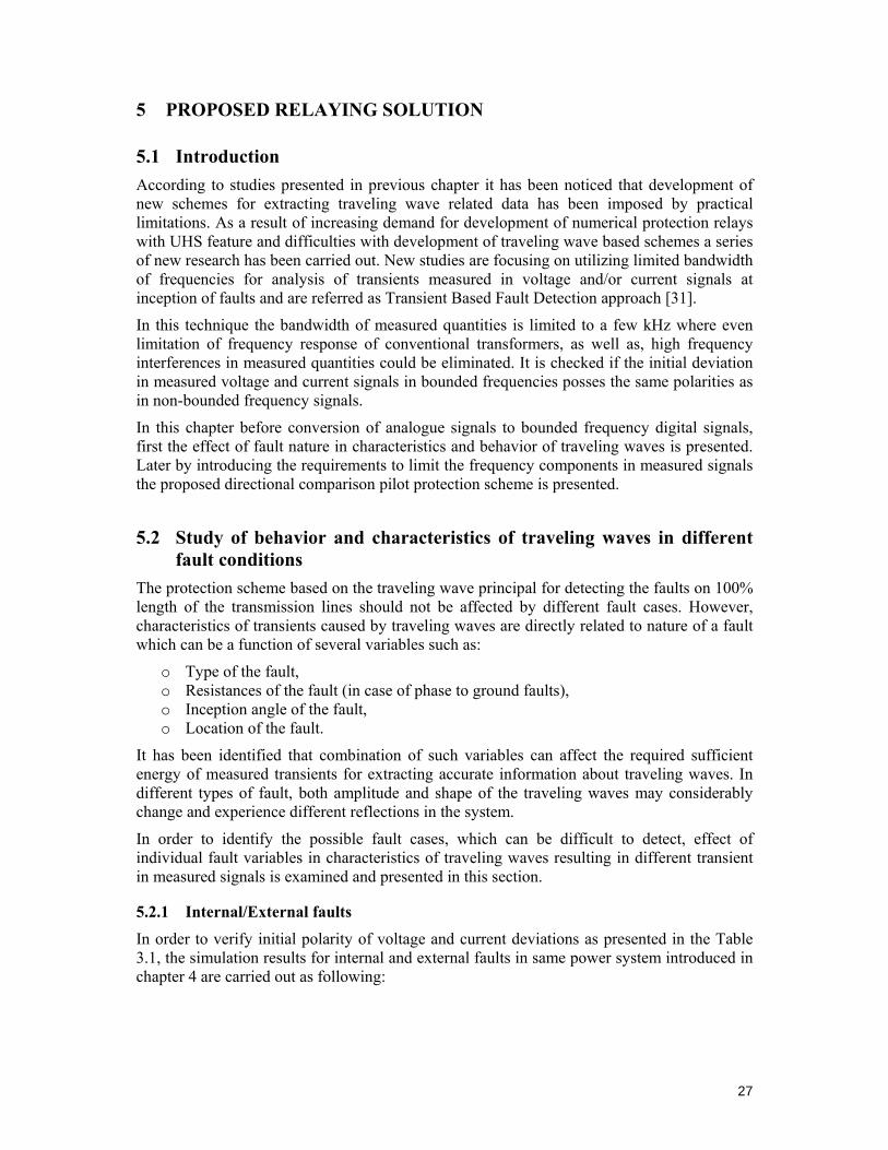
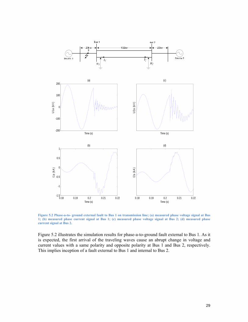
Figure 5.1 Phase-a-to-ground fault at midpoint of transmission line; (a) measured phase voltage signal at Bus 1; (b) measured phase current signal at Bus 1; (c) measured phase voltage signal at Bus 2; (d) measured phase current signal at Bus 2.

Figure 5.1 shows the measured voltage and current signals at Bus 1 and Bus 2, as a result of simulation of a phase-a-to-ground fault internal to Bus 1 and Bus 2. As it is expected, the abrupt changes in voltage and current values start with an opposite sign in measured signals at each end of the line. This indicates arrival of backward traveling waveforms to each terminal which are followed with reflections in the system and result in high frequency transients.

-200

-100

0

100

200

Time (s)

U1a

(kV

)

(a)

Time (s)

U2a

(kV

)

(c)

0.18 0.19 0.2 0.21 0.22-2

-1

0

1

2

3

Time (s)

I1a

(kA

)

(b)

0.18 0.19 0.2 0.21 0.22Time (s)

I2a

(kA

)(d)

29

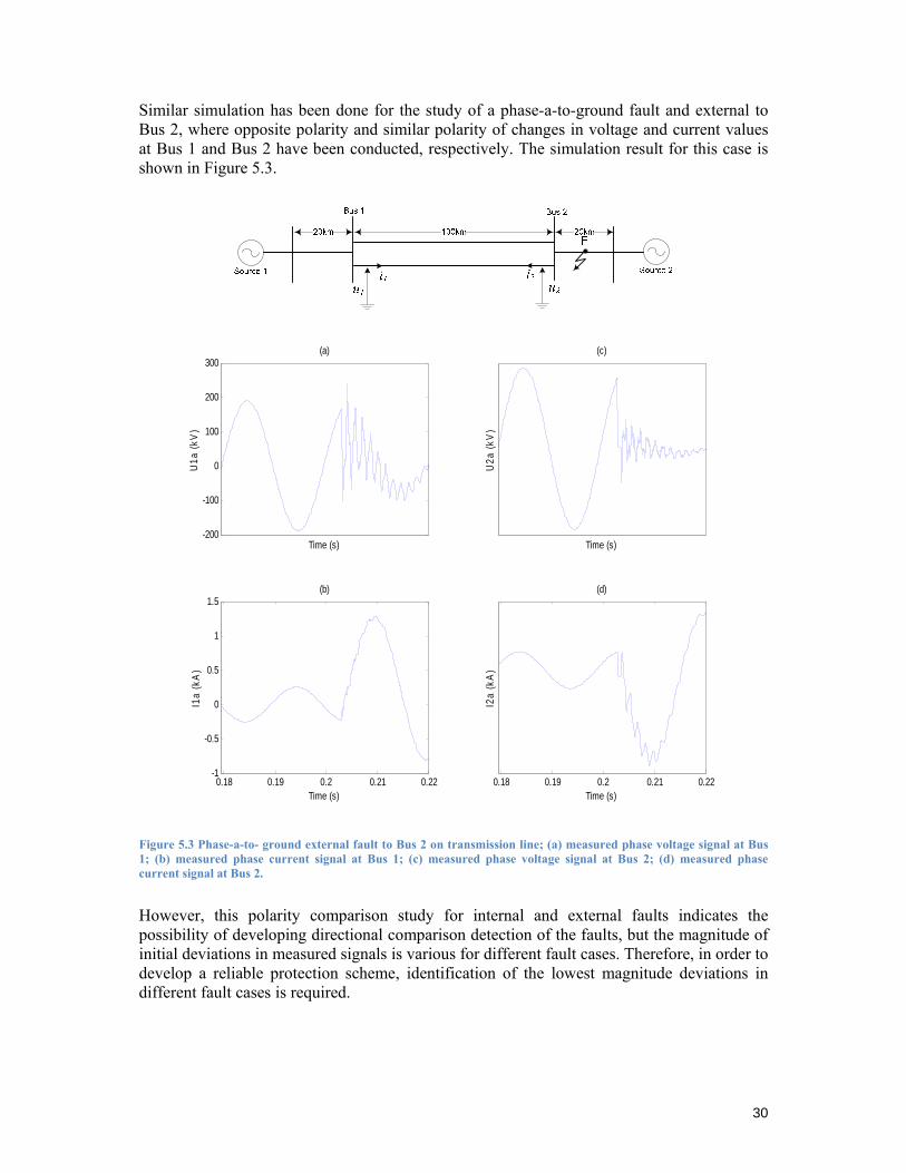
Figure 5.2 Phase-a-to- ground external fault to Bus 1 on transmission line; (a) measured phase voltage signal at Bus 1; (b) measured phase current signal at Bus 1; (c) measured phase voltage signal at Bus 2; (d) measured phase current signal at Bus 2.

Figure 5.2 illustrates the simulation results for phase-a-to-ground fault external to Bus 1. As it is expected, the first arrival of the traveling waves cause an abrupt change in voltage and current values with a same polarity and opposite polarity at Bus 1 and Bus 2, respectively. This implies inception of a fault external to Bus 1 and internal to Bus 2.

-200

-100

0

100

200

Time (s)

U1a

(kV

)

(a)

Time (s)U

2a (k

V)

(c)

0.18 0.19 0.2 0.21 0.22-1.5

-1

-0.5

0

0.5

1

Time (s)

I1a

(kA

)

(b)

0.18 0.19 0.2 0.21 0.22Time (s)

I2a

(kA

)

(d)

30

Similar simulation has been done for the study of a phase-a-to-ground fault and external to Bus 2, where opposite polarity and similar polarity of changes in voltage and current values at Bus 1 and Bus 2 have been conducted, respectively. The simulation result for this case is shown in Figure 5.3.

Figure 5.3 Phase-a-to- ground external fault to Bus 2 on transmission line; (a) measured phase voltage signal at Bus 1; (b) measured phase current signal at Bus 1; (c) measured phase voltage signal at Bus 2; (d) measured phase current signal at Bus 2.

However, this polarity comparison study for internal and external faults indicates the possibility of developing directional comparison detection of the faults, but the magnitude of initial deviations in measured signals is various for different fault cases. Therefore, in order to develop a reliable protection scheme, identification of the lowest magnitude deviations in different fault cases is required.

-200

-100

0

100

200

300

Time (s)

U1a

(kV

)

(a)

Time (s)

U2a

(kV

)

(c)

0.18 0.19 0.2 0.21 0.22-1

-0.5

0

0.5

1

1.5

Time (s)

I1a

(kA

)

(b)

0.18 0.19 0.2 0.21 0.22Time (s)

I2a

(kA

)

(d)

31

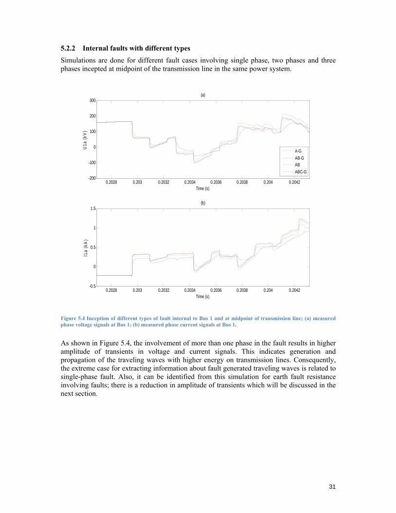
5.2.2 Internal faults with different types

Simulations are done for different fault cases involving single phase, two phases and three phases incepted at midpoint of the transmission line in the same power system.

Figure 5.4 Inception of different types of fault internal to Bus 1 and at midpoint of transmission line; (a) measured phase voltage signals at Bus 1; (b) measured phase current signals at Bus 1.

As shown in Figure 5.4, the involvement of more than one phase in the fault results in higher amplitude of transients in voltage and current signals. This indicates generation and propagation of the traveling waves with higher energy on transmission lines. Consequently, the extreme case for extracting information about fault generated traveling waves is related to single-phase fault. Also, it can be identified from this simulation for earth fault resistance involving faults; there is a reduction in amplitude of transients which will be discussed in the next section.

0.2028 0.203 0.2032 0.2034 0.2036 0.2038 0.204 0.2042-200

-100

0

100

200

300

Time (s)

U1a

(kV

)

(a)

0.2028 0.203 0.2032 0.2034 0.2036 0.2038 0.204 0.2042-0.5

0

0.5

1

1.5

Time (s)

I1a

(kA

)

(b)

A-GAB-GABABC-G

32

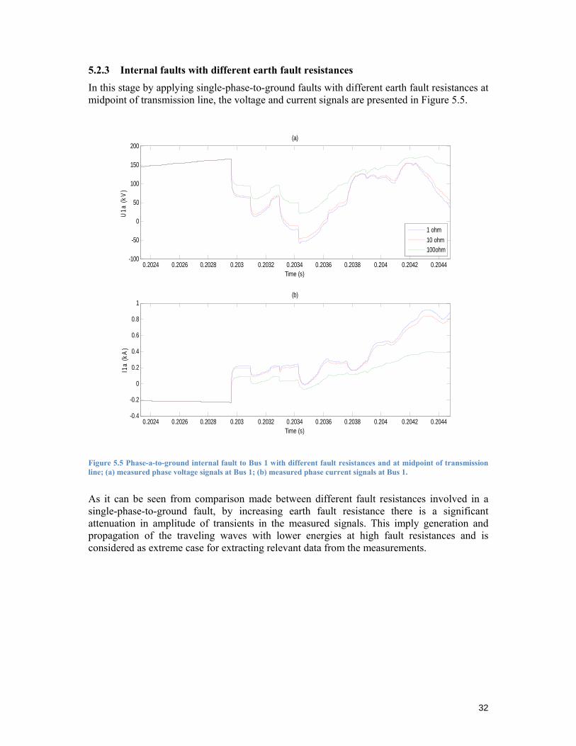
5.2.3 Internal faults with different earth fault resistances

In this stage by applying single-phase-to-ground faults with different earth fault resistances at midpoint of transmission line, the voltage and current signals are presented in Figure 5.5.

Figure 5.5 Phase-a-to-ground internal fault to Bus 1 with different fault resistances and at midpoint of transmission line; (a) measured phase voltage signals at Bus 1; (b) measured phase current signals at Bus 1.

As it can be seen from comparison made between different fault resistances involved in a single-phase-to-ground fault, by increasing earth fault resistance there is a significant attenuation in amplitude of transients in the measured signals. This imply generation and propagation of the traveling waves with lower energies at high fault resistances and is considered as extreme case for extracting relevant data from the measurements.

0.2024 0.2026 0.2028 0.203 0.2032 0.2034 0.2036 0.2038 0.204 0.2042 0.2044-100

-50

0

50

100

150

200

Time (s)

U1a

(kV

)

(a)

0.2024 0.2026 0.2028 0.203 0.2032 0.2034 0.2036 0.2038 0.204 0.2042 0.2044-0.4

-0.2

0

0.2

0.4

0.6

0.8

1

Time (s)

I1a

(kA

)

(b)

1 ohm10 ohm100ohm

33

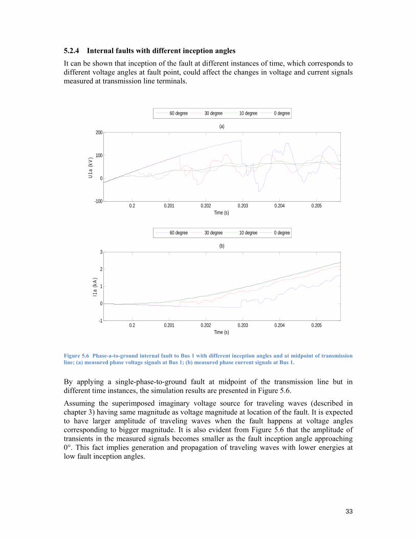
5.2.4 Internal faults with different inception angles

It can be shown that inception of the fault at different instances of time, which corresponds to different voltage angles at fault point, could affect the changes in voltage and current signals measured at transmission line terminals.

Figure 5.6 Phase-a-to-ground internal fault to Bus 1 with different inception angles and at midpoint of transmission line; (a) measured phase voltage signals at Bus 1; (b) measured phase current signals at Bus 1.

By applying a single-phase-to-ground fault at midpoint of the transmission line but in different time instances, the simulation results are presented in Figure 5.6.

Assuming the superimposed imaginary voltage source for traveling waves (described in chapter 3) having same magnitude as voltage magnitude at location of the fault. It is expected to have larger amplitude of traveling waves when the fault happens at voltage angles corresponding to bigger magnitude. It is also evident from Figure 5.6 that the amplitude of transients in the measured signals becomes smaller as the fault inception angle approaching 0°. This fact implies generation and propagation of traveling waves with lower energies at low fault inception angles.

0.2 0.201 0.202 0.203 0.204 0.205-100

0

100

200

Time (s)

U1a

(kV

)

(a)

0.2 0.201 0.202 0.203 0.204 0.205-1

0

1

2

3

Time (s)

I1a

(kA

)

(b)

60 degree 30 degree 10 degree 0 degree

60 degree 30 degree 10 degree 0 degree

34

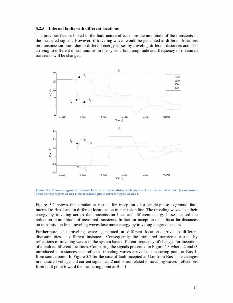
5.2.5 Internal faults with different locations

The previous factors linked to the fault nature affect more the amplitude of the transients in the measured signals. However, if traveling waves would be generated at different locations on transmission lines, due to different energy losses by traveling different distances and also arriving to different discontinuities in the system, both amplitude and frequency of measured transients will be changed.

Figure 5.7 Phase-a-to-ground internal fault at different distances from Bus 1 on transmission line; (a) measured phase voltage signals at Bus 1; (b) measured phase current signals at Bus 1.

Figure 5.7 shows the simulation results for inception of a single-phase-to-ground fault internal to Bus 1 and in different locations on transmission line. The traveling waves lost their energy by traveling across the transmission lines and different energy losses caused the reduction in amplitude of measured transients. In fact for inception of faults at far distances on transmission line, traveling waves lose more energy by traveling longer distances.

Furthermore, the traveling waves generated at different locations arrive to different discontinuities at different instances. Consequently the measured transients caused by reflections of traveling waves in the system have different frequency of changes for inception of a fault at different locations. Comparing the signals presented in Figure 4.3 where t2 and t3 introduced as instances that reflected traveling waves arrived to measuring point at Bus 1, from source point. In Figure 5.7 for the case of fault incepted at 1km from Bus 1 the changes in measured voltage and current signals at t2 and t3 are related to traveling waves’ reflections from fault point toward the measuring point at Bus 1.

0.2028 0.2029 0.2029 0.203 0.203 0.2031-50

0

50

100

150

200

Time (s)

U1a

(kV

)

(a)

0.2028 0.2029 0.2029 0.203 0.203 0.2031-0.4

-0.2

0

0.2

0.4

0.6

Time (s)

I1a

(kA

)

(b)

50km25km10km1km

t2 t

3

t1

t1

t2

t3

35

Therefore, the location of the fault does not only affect the energy level in measured transients but also, introduce a wide range of changing frequency transients for measured signals. In traveling wave numerical relays, which are utilizing digital samples of measured signals, more complicated methods to extract accurate information from wide frequency range of transients are required.

According to this study the combination of two or more extreme cases that identified for faults with individual variables as summarized in Table 5.1, can form the most difficult fault cases to be detected with such protection schemes.

Table 5.1 Extreme fault cases for detection with individual variables

Individual fault variable Extreme case for detection

Type of the fault Single-phase-to-ground

Earth fault resistance High resistance

Fault Inception angle Low inception angle

Location of the fault At far distance from measuring point

This information is used to test the performance of proposed algorithm and also enhanced the finding of tuned threshold levels for reliable fault detections as will be discussed later in this chapter.

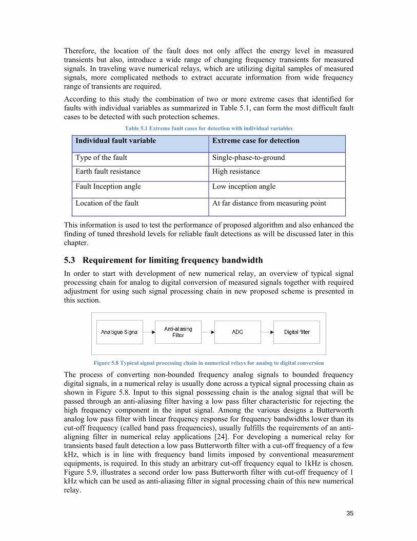
5.3 Requirement for limiting frequency bandwidth In order to start with development of new numerical relay, an overview of typical signal processing chain for analog to digital conversion of measured signals together with required adjustment for using such signal processing chain in new proposed scheme is presented in this section.

Figure 5.8 Typical signal processing chain in numerical relays for analog to digital conversion

The process of converting non-bounded frequency analog signals to bounded frequency digital signals, in a numerical relay is usually done across a typical signal processing chain as shown in Figure 5.8. Input to this signal possessing chain is the analog signal that will be passed through an anti-aliasing filter having a low pass filter characteristic for rejecting the high frequency component in the input signal. Among the various designs a Butterworth analog low pass filter with linear frequency response for frequency bandwidths lower than its cut-off frequency (called band pass frequencies), usually fulfills the requirements of an anti-aligning filter in numerical relay applications [24]. For developing a numerical relay for transients based fault detection a low pass Butterworth filter with a cut-off frequency of a few kHz, which is in line with frequency band limits imposed by conventional measurement equipments, is required. In this study an arbitrary cut-off frequency equal to 1kHz is chosen. Figure 5.9, illustrates a second order low pass Butterworth filter with cut-off frequency of 1 kHz which can be used as anti-aliasing filter in signal processing chain of this new numerical relay.

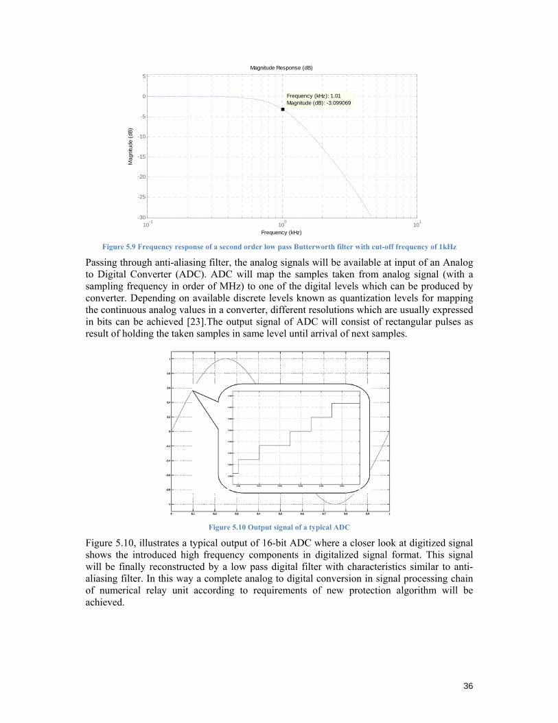
36

Figure 5.9 Frequency response of a second order low pass Butterworth filter with cut-off frequency of 1kHz

Passing through anti-aliasing filter, the analog signals will be available at input of an Analog to Digital Converter (ADC). ADC will map the samples taken from analog signal (with a sampling frequency in order of MHz) to one of the digital levels which can be produced by converter. Depending on available discrete levels known as quantization levels for mapping the continuous analog values in a converter, different resolutions which are usually expressed in bits can be achieved [23].The output signal of ADC will consist of rectangular pulses as result of holding the taken samples in same level until arrival of next samples.

Figure 5.10 Output signal of a typical ADC

Figure 5.10, illustrates a typical output of 16-bit ADC where a closer look at digitized signal shows the introduced high frequency components in digitalized signal format. This signal will be finally reconstructed by a low pass digital filter with characteristics similar to anti-aliasing filter. In this way a complete analog to digital conversion in signal processing chain of numerical relay unit according to requirements of new protection algorithm will be achieved.

10-1

100

101

-30

-25

-20

-15

-10

-5

0

5

Frequency (kHz)

Mag

nitu

de (d

B)

Magnitude Response (dB)

Frequency (kHz): 1.01 Magnitude (dB): -3.099069

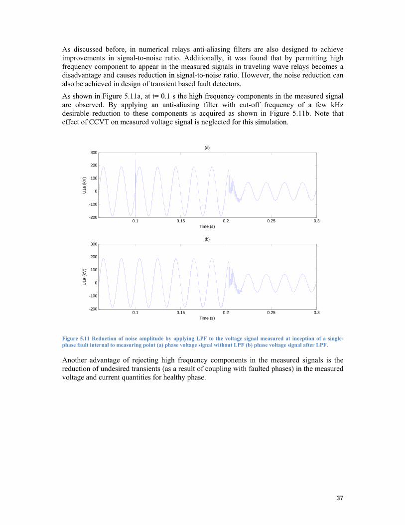
37

As discussed before, in numerical relays anti-aliasing filters are also designed to achieve improvements in signal-to-noise ratio. Additionally, it was found that by permitting high frequency component to appear in the measured signals in traveling wave relays becomes a disadvantage and causes reduction in signal-to-noise ratio. However, the noise reduction can also be achieved in design of transient based fault detectors.

As shown in Figure 5.11a, at t= 0.1 s the high frequency components in the measured signal are observed. By applying an anti-aliasing filter with cut-off frequency of a few kHz desirable reduction to these components is acquired as shown in Figure 5.11b. Note that effect of CCVT on measured voltage signal is neglected for this simulation.

Figure 5.11 Reduction of noise amplitude by applying LPF to the voltage signal measured at inception of a single- phase fault internal to measuring point (a) phase voltage signal without LPF (b) phase voltage signal after LPF.

Another advantage of rejecting high frequency components in the measured signals is the reduction of undesired transients (as a result of coupling with faulted phases) in the measured voltage and current quantities for healthy phase.

0.1 0.15 0.2 0.25 0.3-200

-100

0

100

200

300

Time (s)

U1a

(kV

)

(a)

0.1 0.15 0.2 0.25 0.3-200

-100

0

100

200

300

Time (s)

U1a

(kV

)

(b)

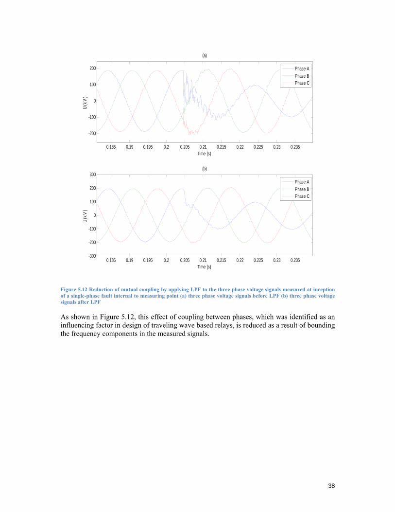
38

Figure 5.12 Reduction of mutual coupling by applying LPF to the three phase voltage signals measured at inception of a single-phase fault internal to measuring point (a) three phase voltage signals before LPF (b) three phase voltage signals after LPF

As shown in Figure 5.12, this effect of coupling between phases, which was identified as an influencing factor in design of traveling wave based relays, is reduced as a result of bounding the frequency components in the measured signals.

0.185 0.19 0.195 0.2 0.205 0.21 0.215 0.22 0.225 0.23 0.235

-200

-100

0

100

200

Time (s)

U(k

V)

(a)

0.185 0.19 0.195 0.2 0.205 0.21 0.215 0.22 0.225 0.23 0.235-300

-200

-100

0

100

200

300

Time (s)

U(k

V)

(b)

Phase APhase BPhase C

Phase APhase BPhase C

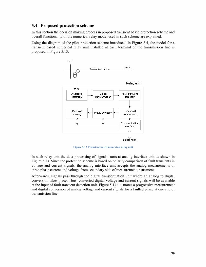
39

5.4 Proposed protection scheme In this section the decision making process in proposed transient based protection scheme and overall functionality of the numerical relay model used in such scheme are explained.

Using the diagram of the pilot protection scheme introduced in Figure 2.4, the model for a transient based numerical relay unit installed at each terminal of the transmission line is proposed in Figure 5.13.

Figure 5.13 Transient based numerical relay unit

In such relay unit the data processing of signals starts at analog interface unit as shown in Figure 5.13. Since the protection scheme is based on polarity comparison of fault transients in voltage and current signals, the analog interface unit accepts the analog measurements of three-phase current and voltage from secondary side of measurement instruments.

Afterwards, signals pass through the digital transformation unit where an analog to digital conversion takes place. Thus, converted digital voltage and current signals will be available at the input of fault transient detection unit. Figure 5.14 illustrates a progressive measurement and digital conversion of analog voltage and current signals for a faulted phase at one end of transmission line.

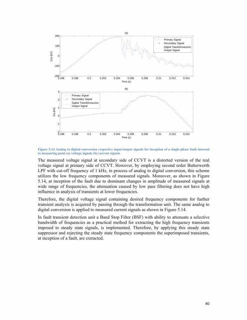
40

Figure 5.14 Analog to digital conversion respective input/output signals for inception of a single-phase fault internal to measuring point (a) voltage signals (b) current signals

The measured voltage signal at secondary side of CCVT is a distorted version of the real voltage signal at primary side of CCVT. However, by employing second order Butterworth LPF with cut-off frequency of 1 kHz, in process of analog to digital conversion, this scheme utilizes the low frequency components of measured signals. Moreover, as shown in Figure 5.14, at inception of the fault due to dominant changes in amplitude of measured signals at wide range of frequencies, the attenuation caused by low pass filtering does not have high influence in analysis of transients at lower frequencies.

Therefore, the digital voltage signal containing desired frequency components for further transient analysis is acquired by passing through the transformation unit. The same analog to digital conversion is applied to measured current signals as shown in Figure 5.14.

In fault transient detection unit a Band Stop Filter (BSF) with ability to attenuate a selective bandwidth of frequencies as a practical method for extracting the high frequency transients imposed to steady state signals, is implemented. Therefore, by applying this steady state suppressor and rejecting the steady state frequency components the superimposed transients, at inception of a fault, are extracted.

0.196 0.198 0.2 0.202 0.204 0.206 0.208 0.21 0.212 0.214-200

-100

0

100

200

Time (s)

U1a

(kV

)

(a)

0.196 0.198 0.2 0.202 0.204 0.206 0.208 0.21 0.212 0.214-2

-1

0

1

2

3

Time (s)

I1a

(kA

)

(b)

Primary SignalSecondary SignalDigital TransformassionOutput Signal

Primary SignalSecondary SignalDigital TransformassionOutput Signal

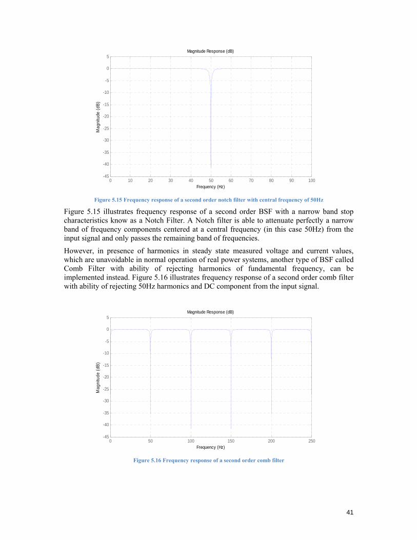
41

Figure 5.15 Frequency response of a second order notch filter with central frequency of 50Hz

Figure 5.15 illustrates frequency response of a second order BSF with a narrow band stop characteristics know as a Notch Filter. A Notch filter is able to attenuate perfectly a narrow band of frequency components centered at a central frequency (in this case 50Hz) from the input signal and only passes the remaining band of frequencies.

However, in presence of harmonics in steady state measured voltage and current values, which are unavoidable in normal operation of real power systems, another type of BSF called Comb Filter with ability of rejecting harmonics of fundamental frequency, can be implemented instead. Figure 5.16 illustrates frequency response of a second order comb filter with ability of rejecting 50Hz harmonics and DC component from the input signal.

Figure 5.16 Frequency response of a second order comb filter

0 10 20 30 40 50 60 70 80 90 100-45

-40

-35

-30

-25

-20

-15

-10

-5

0

5

Frequency (Hz)

Mag

nitu

de (d

B)

Magnitude Response (dB)

0 50 100 150 200 250-45

-40

-35

-30

-25

-20

-15

-10

-5

0

5

Frequency (Hz)

Mag

nitu

de (d

B)

Magnitude Response (dB)

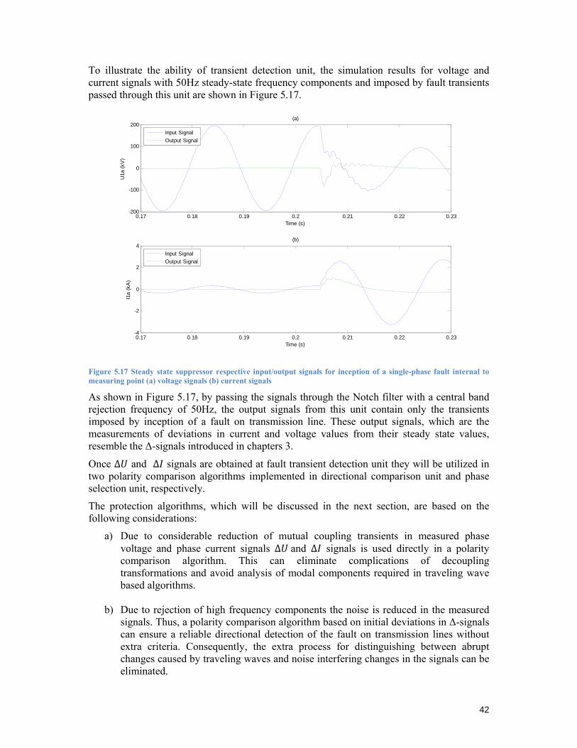
42

To illustrate the ability of transient detection unit, the simulation results for voltage and current signals with 50Hz steady-state frequency components and imposed by fault transients passed through this unit are shown in Figure 5.17.

Figure 5.17 Steady state suppressor respective input/output signals for inception of a single-phase fault internal to measuring point (a) voltage signals (b) current signals

As shown in Figure 5.17, by passing the signals through the Notch filter with a central band rejection frequency of 50Hz, the output signals from this unit contain only the transients imposed by inception of a fault on transmission line. These output signals, which are the measurements of deviations in current and voltage values from their steady state values, resemble the Δ-signals introduced in chapters 3.

Once ∆ and ∆ signals are obtained at fault transient detection unit they will be utilized in two polarity comparison algorithms implemented in directional comparison unit and phase selection unit, respectively.

The protection algorithms, which will be discussed in the next section, are based on the following considerations:

a) Due to considerable reduction of mutual coupling transients in measured phase voltage and phase current signals ∆ and ∆ signals is used directly in a polarity comparison algorithm. This can eliminate complications of decoupling transformations and avoid analysis of modal components required in traveling wave based algorithms.

b) Due to rejection of high frequency components the noise is reduced in the measured signals. Thus, a polarity comparison algorithm based on initial deviations in Δ-signals can ensure a reliable directional detection of the fault on transmission lines without extra criteria. Consequently, the extra process for distinguishing between abrupt changes caused by traveling waves and noise interfering changes in the signals can be eliminated.

0.17 0.18 0.19 0.2 0.21 0.22 0.23-200

-100

0

100

200

Time (s)

U1a

(kV

)(a)

0.17 0.18 0.19 0.2 0.21 0.22 0.23-4

-2

0

2

4

Time (s)

I1a

(kA

)

(b)

Input SignalOutput Signal

Input SignalOutput Signal

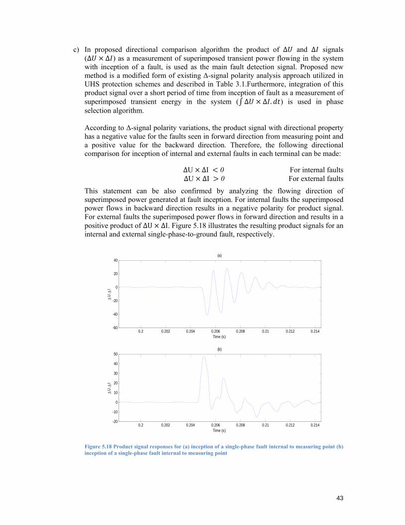
43

c) In proposed directional comparison algorithm the product of ∆ and ∆ signals (∆ ∆ ) as a measurement of superimposed transient power flowing in the system with inception of a fault, is used as the main fault detection signal. Proposed new method is a modified form of existing Δ-signal polarity analysis approach utilized in UHS protection schemes and described in Table 3.1.Furthermore, integration of this product signal over a short period of time from inception of fault as a measurement of superimposed transient energy in the system ( ∆ ∆ . ) is used in phase selection algorithm. According to Δ-signal polarity variations, the product signal with directional property has a negative value for the faults seen in forward direction from measuring point and a positive value for the backward direction. Therefore, the following directional comparison for inception of internal and external faults in each terminal can be made:

∆U ∆I 0 For internal faults ∆U ∆I 0 For external faults

This statement can be also confirmed by analyzing the flowing direction of superimposed power generated at fault inception. For internal faults the superimposed power flows in backward direction results in a negative polarity for product signal. For external faults the superimposed power flows in forward direction and results in a positive product of ∆U ∆I. Figure 5.18 illustrates the resulting product signals for an internal and external single-phase-to-ground fault, respectively.

Figure 5.18 Product signal responses for (a) inception of a single-phase fault internal to measuring point (b) inception of a single-phase fault internal to measuring point

0.2 0.202 0.204 0.206 0.208 0.21 0.212 0.214-60

-40

-20

0

20

40

Time (s)

ΔU

. ΔI

(a)

0.2 0.202 0.204 0.206 0.208 0.21 0.212 0.214-20

-10

0

10

20

30

40

50

Time (s)

ΔU

. ΔI

(b)

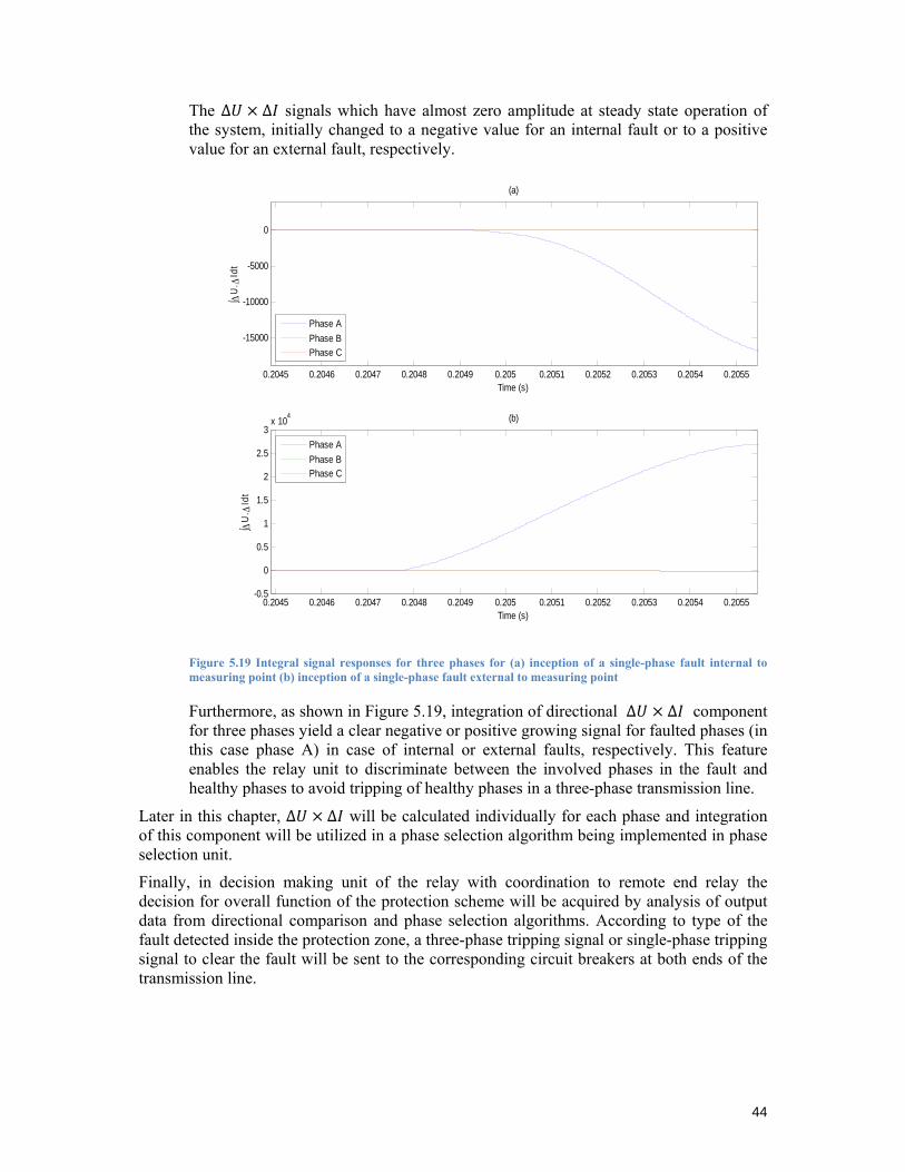
44

The ∆ ∆ signals which have almost zero amplitude at steady state operation of the system, initially changed to a negative value for an internal fault or to a positive value for an external fault, respectively.

Figure 5.19 Integral signal responses for three phases for (a) inception of a single-phase fault internal to measuring point (b) inception of a single-phase fault external to measuring point

Furthermore, as shown in Figure 5.19, integration of directional ∆ ∆ component for three phases yield a clear negative or positive growing signal for faulted phases (in this case phase A) in case of internal or external faults, respectively. This feature enables the relay unit to discriminate between the involved phases in the fault and healthy phases to avoid tripping of healthy phases in a three-phase transmission line.

Later in this chapter, ∆ ∆ will be calculated individually for each phase and integration of this component will be utilized in a phase selection algorithm being implemented in phase selection unit.

Finally, in decision making unit of the relay with coordination to remote end relay the decision for overall function of the protection scheme will be acquired by analysis of output data from directional comparison and phase selection algorithms. According to type of the fault detected inside the protection zone, a three-phase tripping signal or single-phase tripping signal to clear the fault will be sent to the corresponding circuit breakers at both ends of the transmission line.

0.2045 0.2046 0.2047 0.2048 0.2049 0.205 0.2051 0.2052 0.2053 0.2054 0.2055

-15000

-10000

-5000

0

Time (s)

∫ΔU

. ΔId

t

(a)

0.2045 0.2046 0.2047 0.2048 0.2049 0.205 0.2051 0.2052 0.2053 0.2054 0.2055-0.5

0

0.5

1

1.5

2

2.5

3x 104

Time (s)

∫ΔU

. ΔId

t

(b)

Phase APhase BPhase C

Phase APhase BPhase C

45

5.4.1 Developed algorithms

In this section protection algorithms implemented in directional comparison unit and phase selection unit are presented in details. In the proposed protection scheme three groups of protection elements together with a group of threshold elements are defined in the algorithm as following:

o Fault detection elements ( Trip1 and Trip2), o Directional detection elements (F_external and F_internal), o Phase selection elements (a_trip,b_trip,c_trip,ab_trip,ac_trip,bc_trip and abc_trip), o Threshold elements ( 1 and 2).

5.4.1.1 Directional comparison algorithm

As it was discussed in previous section, the product of ∆ ∆ is utilized as directional comparison signal in this algorithm. By real time monitoring of this signal and introducing a negative threshold level, when the magnitude reaches the levels greater than the threshold level, the internal fault detection can be determined by the local relay. However, as it was observed from Figure 5.18, the first deviation in ∆ ∆ signal from zero level, for either internal or external fault, is followed by other changing levels reaching positive and negative values. These variations in the product signal continuing in a short period of time (depending on power system configuration up to one cycle of power frequency e.g. 10ms) after inception of a fault are originally linked to the imposed transients due to generation and reflection of traveling waves in the system.

Thus, a priority for detection of external faults should be set in order to utilize such product signal in a directional comparison algorithm and to avoid wrong directional detections. In this case initial positive deviation at ∆ ∆ signal could be followed by transients crossing the negative threshold level introduced for detection of internal faults. Consequently, the polarity comparison shall be based on initial crossing of ∆ ∆ signal with the threshold levels and all subsequent crossings shall be disregarded in directional detection decision.

The developed directional algorithm implemented in directional comparison unit of the numerical relay is presented as the flowchart in Figure 5.20. As shown in Figure 5.20, the algorithm starts with setting the directional detection elements as well as integrator operators to zero and later reads the voltage and current Δ-signals, which are available at input of the directional comparison unit.

Afterwards, the polarity comparison algorithm based on individual logics for directional comparison components calculated for each phase with priority to positive polarity detections is developed. This algorithm utilizes three polarity comparison functions for external fault detection logic and three polarity comparison functions for internal fault detections logic. Furthermore, the same threshold levels are defined in negative and positive planes (Setting criteria of threshold value 1which is a negative value will be discussed in the next chapter).

In the cases of more than one phase being involved in a fault, due to phase difference among the three phases, inception angle of fault can have different values for different phases resulting in propagation of traveling waves with a variety of shapes and energy levels in the system. Therefore, the fault transients appearing with the highest rate of changes trigger first the polarity comparison logics. Thus, an overall increase in the relaying response will be achieved.

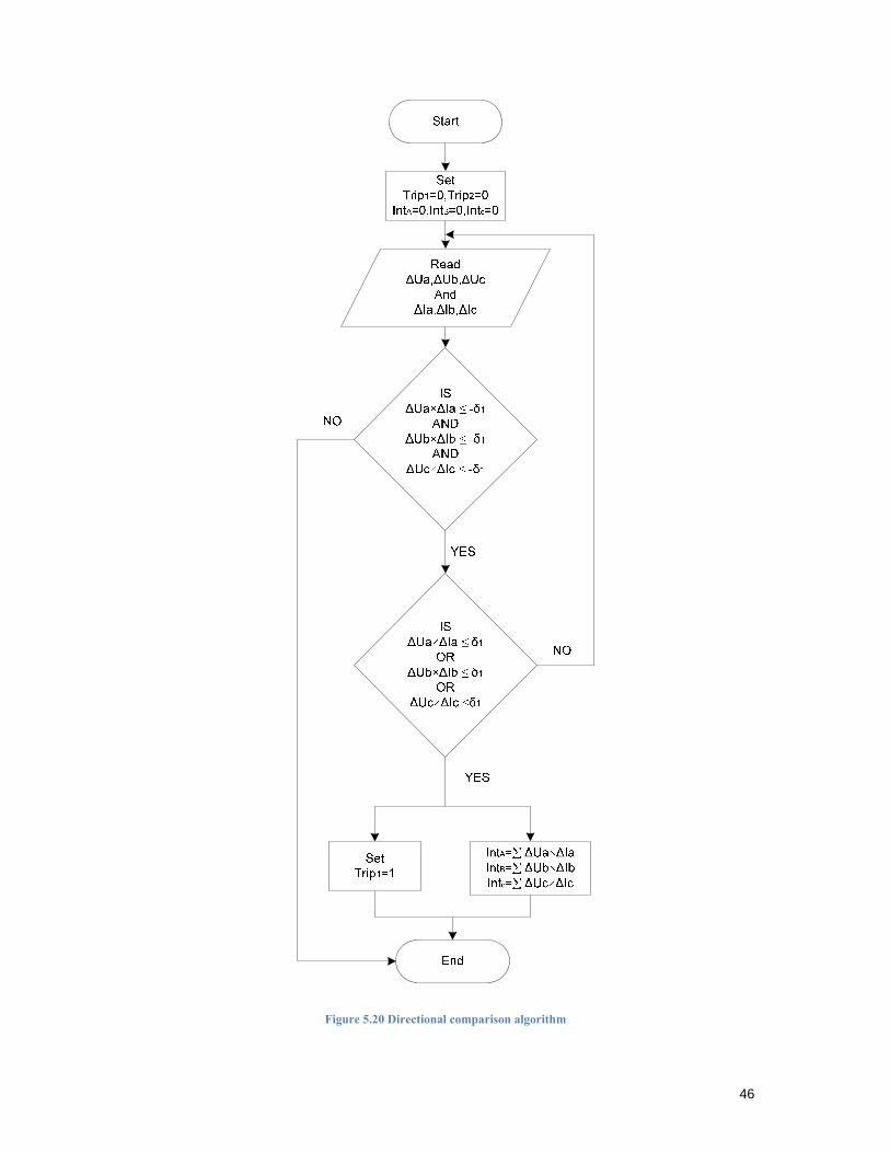
46

Figure 5.20 Directional comparison algorithm

47

By individual real time monitoring of ∆ ∆ signals for each phase, an external fault will be concluded if one of the external fault detection comparison functions becomes zero. However, the internal fault will be only concluded if one of the internal comparison functions becomes non-zero while all external fault detection comparison functions are non-zero. In this directional comparison algorithm, only the fault detection elements will be set to 1 in case of inception of an internal fault prior to inception of an external fault.

Finally, after detection of an internal fault, the local fault detection element (Trip 1) will be set to 1, and the local relay has to wait for reading the new value of the remote detection element (Trip 2) to be transmitted via a communication link. Meanwhile, three accumulating operators for three phases start to accumulate the measured samples in ∆ ∆ signals which form the integral signals required for phase selection algorithm, as it will be described in the next section. Note that integral operators will be triggered only by detection of internal faults and therefore will have only negative growing values in this scheme.

5.4.1.2 Phase selection algorithm

The phase selection algorithm, as shown below in Figure 5.21, starts by setting the directional detection elements as well as phase selection elements to 0. Then relay reads the local fault detection element (Trip1) from directional comparison unit and remote fault detection element (Trip 2) which is received from remote relay over the communication link between two relays.

Once fault detection elements from both relays are available, a comparison between states of the incepted fault seen from both ends induces the formation of the directional detection elements. In case of an external fault to protected zone, a non-zero directional element related to external fault (F-external) will be sent directly to decision making unit. However, in case of an internal fault the non-zero directional element related to internal fault (F_internal =1) will initiate comparison of integral signals (which are calculated meanwhile) with a negative threshold value 2 in a sequence as shown in Figure 5.21. For example in case of a phase-a-to-phase-b fault only phase selection element ab_trip will be set to 1 since only integral signals related to these two phases (intA and intB) cross the threshold values. Finally, the directional detection element related to internal fault and the phase selection element related to faulted phases will be sent to decision making unit of the local relay.

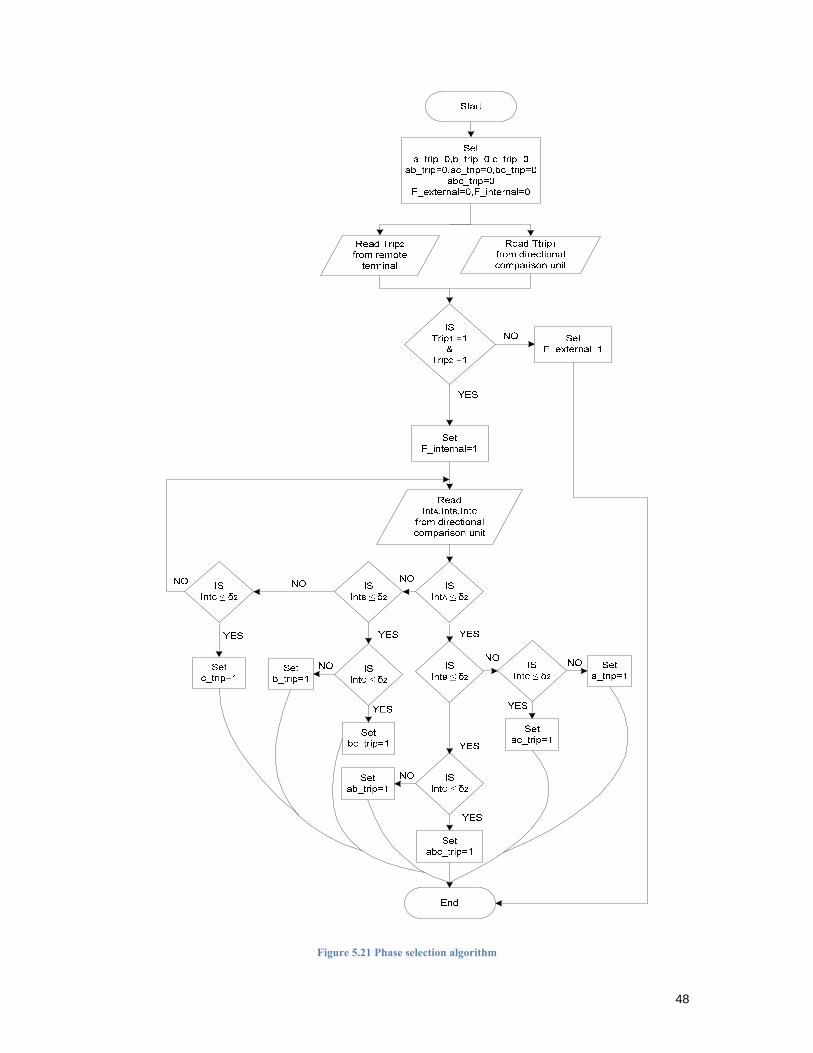
48

Figure 5.21 Phase selection algorithm

49

Protection algorithm explained in this section consists of two individual algorithms for directional comparison and phase selection, respectively. ∆ ∆ signals are integrated in directional comparison algorithm and ∆ ∆ . signals are used in phase selection algorithm, respectively.

However, this scheme is not applicable for detection of simultaneous faults where the protection algorithm is blocked for an external fault. Feasibility of rearrangements of this proposed algorithm by employing the phase selection elements for both fault detection and phase selection purpose in developing a non-blocking scheme has been found. As shown in Figure 5.19 by monitoring the growing values of integral signals after inception of a fault on transmission line, discrimination between internal faults from external faults is possible. In case of internal fault the integral signal ∆ ∆ . has a negative growing value and a positive growing value for the external fault. But utilizing an integral function, which can be triggered and start to grow even for small changes in Δ-signals without inception of faults, is not desired.

The modified algorithm can be found in Appendix 3, in which by removing the polarity comparison logic for positive polarity detection and using the ∆ ∆ signals only for detection of faults, triggering of accumulators at non fault conditions can be avoided. Thus, in this new condition comparison of fault detection elements does not form directional detection elements anymore. As it can be seen in the modified phase selection algorithm in the Appendix 3, the phase selection elements only will be sent to decision making unit by crossing the negative threshold value 2. This happens for inception of internal faults and no extra logic is required for distinguishing internal faults from external faults. Finally, in order to take a decision about the detected faults at local relay and a reliable phase selection, the local phase selection elements will be compared with the remote phase selection elements.

Disadvantage of this scheme is the delay introduced for final decision making due to exchange of phase selection elements. Since the slope of changes between the measured data in integral signals is not very high (in comparison to product signals), it takes longer period of time for integral signals to reach the threshold level. Therefore, possible improvements in non blocking schemes shall be done as a future work to reach UHS relaying feature.

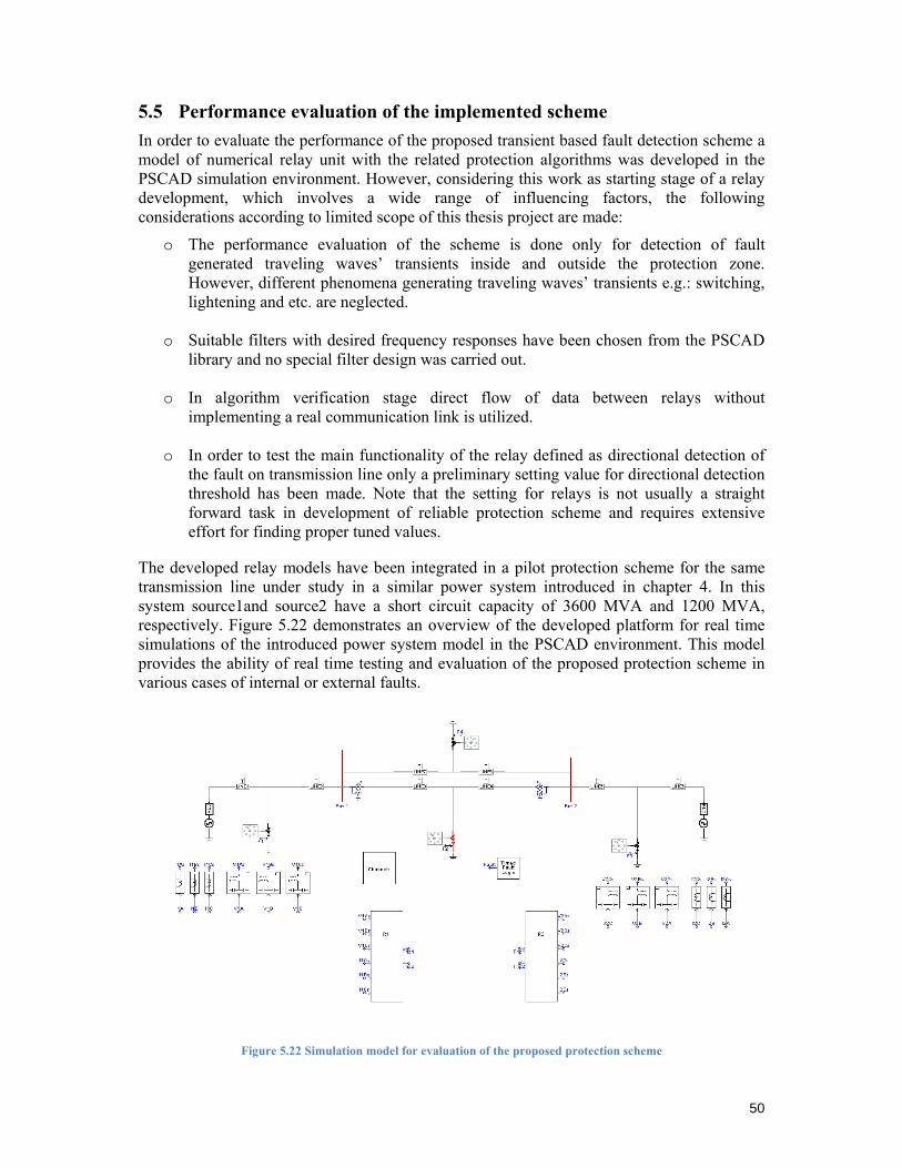
50

5.5 Performance evaluation of the implemented scheme In order to evaluate the performance of the proposed transient based fault detection scheme a model of numerical relay unit with the related protection algorithms was developed in the PSCAD simulation environment. However, considering this work as starting stage of a relay development, which involves a wide range of influencing factors, the following considerations according to limited scope of this thesis project are made:

o The performance evaluation of the scheme is done only for detection of fault generated traveling waves’ transients inside and outside the protection zone. However, different phenomena generating traveling waves’ transients e.g.: switching, lightening and etc. are neglected.

o Suitable filters with desired frequency responses have been chosen from the PSCAD library and no special filter design was carried out.

o In algorithm verification stage direct flow of data between relays without implementing a real communication link is utilized.

o In order to test the main functionality of the relay defined as directional detection of the fault on transmission line only a preliminary setting value for directional detection threshold has been made. Note that the setting for relays is not usually a straight forward task in development of reliable protection scheme and requires extensive effort for finding proper tuned values.

The developed relay models have been integrated in a pilot protection scheme for the same transmission line under study in a similar power system introduced in chapter 4. In this system source1and source2 have a short circuit capacity of 3600 MVA and 1200 MVA, respectively. Figure 5.22 demonstrates an overview of the developed platform for real time simulations of the introduced power system model in the PSCAD environment. This model provides the ability of real time testing and evaluation of the proposed protection scheme in various cases of internal or external faults.

Figure 5.22 Simulation model for evaluation of the proposed protection scheme

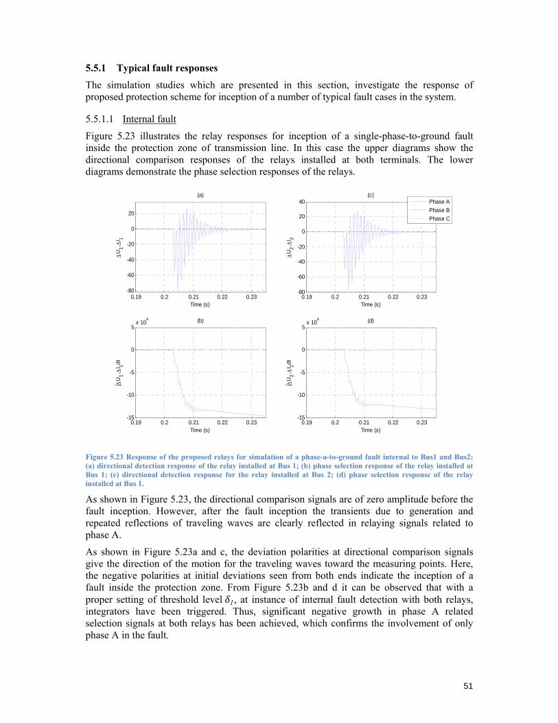
51

5.5.1 Typical fault responses

The simulation studies which are presented in this section, investigate the response of proposed protection scheme for inception of a number of typical fault cases in the system.

5.5.1.1 Internal fault

Figure 5.23 illustrates the relay responses for inception of a single-phase-to-ground fault inside the protection zone of transmission line. In this case the upper diagrams show the directional comparison responses of the relays installed at both terminals. The lower diagrams demonstrate the phase selection responses of the relays.

Figure 5.23 Response of the proposed relays for simulation of a phase-a-to-ground fault internal to Bus1 and Bus2; (a) directional detection response of the relay installed at Bus 1; (b) phase selection response of the relay installed at Bus 1; (c) directional detection response for the relay installed at Bus 2; (d) phase selection response of the relay installed at Bus 1.

As shown in Figure 5.23, the directional comparison signals are of zero amplitude before the fault inception. However, after the fault inception the transients due to generation and repeated reflections of traveling waves are clearly reflected in relaying signals related to phase A.

As shown in Figure 5.23a and c, the deviation polarities at directional comparison signals give the direction of the motion for the traveling waves toward the measuring points. Here, the negative polarities at initial deviations seen from both ends indicate the inception of a fault inside the protection zone. From Figure 5.23b and d it can be observed that with a proper setting of threshold level 1, at instance of internal fault detection with both relays, integrators have been triggered. Thus, significant negative growth in phase A related selection signals at both relays has been achieved, which confirms the involvement of only phase A in the fault.

0.19 0.2 0.21 0.22 0.23-80

-60

-40

-20

0

20

Time (s)

ΔU

1. ΔI 1

(a)

0.19 0.2 0.21 0.22 0.23-15

-10

-5

0

5x 10

4

Time (s)

∫ΔU

1. ΔI 1dt

(b)

0.19 0.2 0.21 0.22 0.23-80

-60

-40

-20

0

20

40

Time (s)

ΔU

2. ΔI 2

(c)

0.19 0.2 0.21 0.22 0.23-15

-10

-5

0

5x 10

4

Time (s)

∫ΔU

2. ΔI 2dt

(d)

Phase APhase BPhase C

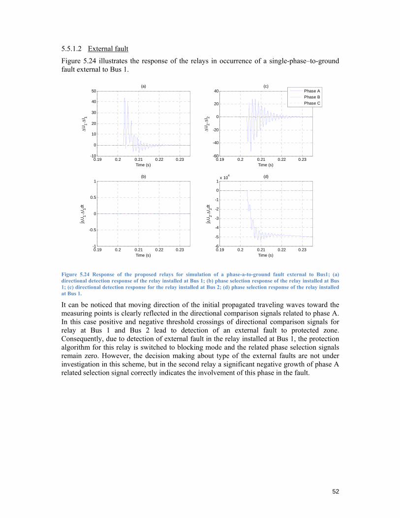
52

5.5.1.2 External fault

Figure 5.24 illustrates the response of the relays in occurrence of a single-phase–to-ground fault external to Bus 1.

Figure 5.24 Response of the proposed relays for simulation of a phase-a-to-ground fault external to Bus1; (a) directional detection response of the relay installed at Bus 1; (b) phase selection response of the relay installed at Bus 1; (c) directional detection response for the relay installed at Bus 2; (d) phase selection response of the relay installed at Bus 1.

It can be noticed that moving direction of the initial propagated traveling waves toward the measuring points is clearly reflected in the directional comparison signals related to phase A. In this case positive and negative threshold crossings of directional comparison signals for relay at Bus 1 and Bus 2 lead to detection of an external fault to protected zone. Consequently, due to detection of external fault in the relay installed at Bus 1, the protection algorithm for this relay is switched to blocking mode and the related phase selection signals remain zero. However, the decision making about type of the external faults are not under investigation in this scheme, but in the second relay a significant negative growth of phase A related selection signal correctly indicates the involvement of this phase in the fault.

0.19 0.2 0.21 0.22 0.23-10

0

10

20

30

40

50

Time (s)

ΔU

1. ΔI 1

(a)

0.19 0.2 0.21 0.22 0.23-1

-0.5

0

0.5

1

Time (s)

∫ΔU

1. ΔI 1dt

(b)

0.19 0.2 0.21 0.22 0.23-60

-40

-20

0

20

40

Time (s)

ΔU

2. ΔI 2

(c)

0.19 0.2 0.21 0.22 0.23-6

-5

-4

-3

-2

-1

0

1x 10

4

Time (s)

∫ΔU

2. ΔI 2dt

(d)

Phase APhase BPhase C

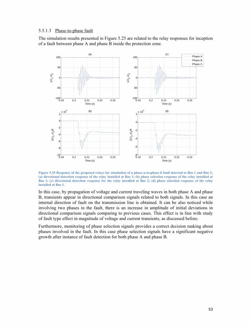
53

5.5.1.3 Phase-to-phase fault

The simulation results presented in Figure 5.25 are related to the relay responses for inception of a fault between phase A and phase B inside the protection zone.

Figure 5.25 Response of the proposed relays for simulation of a phase-a-to-phase-b fault internal to Bus 1 and Bus 2; (a) directional detection response of the relay installed at Bus 1; (b) phase selection response of the relay installed at Bus 1; (c) directional detection response for the relay installed at Bus 2; (d) phase selection response of the relay installed at Bus 1.

In this case, by propagation of voltage and current traveling waves in both phase A and phase B, transients appear in directional comparison signals related to both signals. In this case an internal direction of fault on the transmission line is obtained. It can be also noticed while involving two phases in the fault, there is an increase in amplitude of initial deviations in directional comparison signals comparing to previous cases. This effect is in line with study of fault type effect in magnitude of voltage and current transients, as discussed before.

Furthermore, monitoring of phase selection signals provides a correct decision making about phases involved in the fault. In this case phase selection signals have a significant negative growth after instance of fault detection for both phase A and phase B.

0.19 0.2 0.21 0.22 0.23-100

-50

0

50

100

Time (s)

ΔU

1. ΔI 1

(a)

0.19 0.2 0.21 0.22 0.23-10

-8

-6

-4

-2

0

2x 10

4

Time (s)

∫ΔU

1. ΔI 1dt

(b)

0.19 0.2 0.21 0.22 0.23-100

-50

0

50

100

Time (s)

ΔU

2. ΔI 2

(c)

0.19 0.2 0.21 0.22 0.23-8

-6

-4

-2

0

2x 10

4

Time (s)

∫ΔU

2. ΔI 2dt

(d)

Phase APhase BPhase C

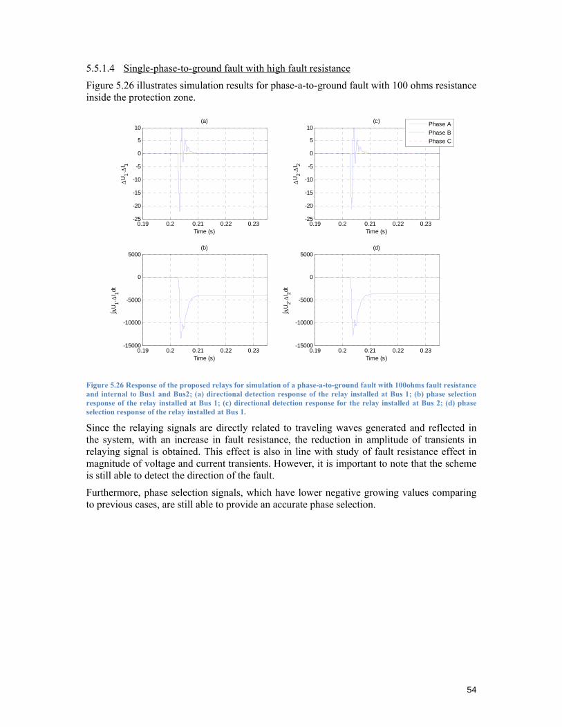
54

5.5.1.4 Single-phase-to-ground fault with high fault resistance

Figure 5.26 illustrates simulation results for phase-a-to-ground fault with 100 ohms resistance inside the protection zone.

Figure 5.26 Response of the proposed relays for simulation of a phase-a-to-ground fault with 100ohms fault resistance and internal to Bus1 and Bus2; (a) directional detection response of the relay installed at Bus 1; (b) phase selection response of the relay installed at Bus 1; (c) directional detection response for the relay installed at Bus 2; (d) phase selection response of the relay installed at Bus 1.

Since the relaying signals are directly related to traveling waves generated and reflected in the system, with an increase in fault resistance, the reduction in amplitude of transients in relaying signal is obtained. This effect is also in line with study of fault resistance effect in magnitude of voltage and current transients. However, it is important to note that the scheme is still able to detect the direction of the fault.

Furthermore, phase selection signals, which have lower negative growing values comparing to previous cases, are still able to provide an accurate phase selection.

0.19 0.2 0.21 0.22 0.23-25

-20

-15

-10

-5

0

5

10

Time (s)

ΔU

1. ΔI 1

(a)

0.19 0.2 0.21 0.22 0.23-15000

-10000

-5000

0

5000

Time (s)

∫ΔU

1. ΔI 1dt

(b)

0.19 0.2 0.21 0.22 0.23-25

-20

-15

-10

-5

0

5

10

Time (s)

ΔU

2. ΔI 2

(c)

0.19 0.2 0.21 0.22 0.23-15000

-10000

-5000

0

5000

Time (s)

∫ΔU

2. ΔI 2dt

(d)

Phase APhase BPhase C

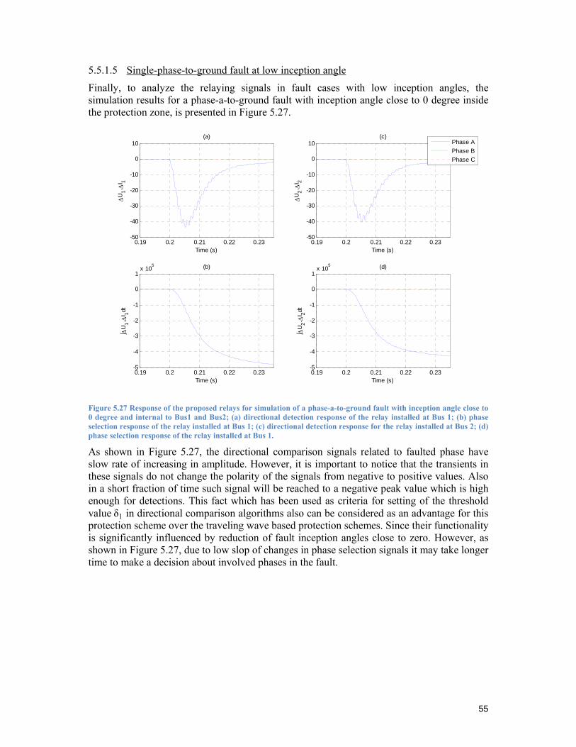
55

5.5.1.5 Single-phase-to-ground fault at low inception angle

Finally, to analyze the relaying signals in fault cases with low inception angles, the simulation results for a phase-a-to-ground fault with inception angle close to 0 degree inside the protection zone, is presented in Figure 5.27.

Figure 5.27 Response of the proposed relays for simulation of a phase-a-to-ground fault with inception angle close to 0 degree and internal to Bus1 and Bus2; (a) directional detection response of the relay installed at Bus 1; (b) phase selection response of the relay installed at Bus 1; (c) directional detection response for the relay installed at Bus 2; (d) phase selection response of the relay installed at Bus 1.

As shown in Figure 5.27, the directional comparison signals related to faulted phase have slow rate of increasing in amplitude. However, it is important to notice that the transients in these signals do not change the polarity of the signals from negative to positive values. Also in a short fraction of time such signal will be reached to a negative peak value which is high enough for detections. This fact which has been used as criteria for setting of the threshold value δ1 in directional comparison algorithms also can be considered as an advantage for this protection scheme over the traveling wave based protection schemes. Since their functionality is significantly influenced by reduction of fault inception angles close to zero. However, as shown in Figure 5.27, due to low slop of changes in phase selection signals it may take longer time to make a decision about involved phases in the fault.

0.19 0.2 0.21 0.22 0.23-50

-40

-30

-20

-10

0

10

Time (s)

ΔU

1. ΔI 1

(a)

0.19 0.2 0.21 0.22 0.23-5

-4

-3

-2

-1

0

1x 10

5

Time (s)

∫ΔU

1. ΔI 1dt

(b)

0.19 0.2 0.21 0.22 0.23-50

-40

-30

-20

-10

0

10

Time (s)

ΔU

2. ΔI 2

(c)

0.19 0.2 0.21 0.22 0.23-5

-4

-3

-2

-1

0

1x 10

5

Time (s)

∫ΔU

2. ΔI 2dt

(d)

Phase APhase BPhase C

56

5.5.2 Testing results

In order to test functionality of the proposed transmission line protection scheme for a large number of fault cases with combination of different factors, as introduced before, a setting approach had to be employed for tuning the directional detection threshold level.

As it is mentioned before, the lowest negative peak value of directional detection signals in all the fault cases with combination of different factors can identify the extreme case of the faults for detection. Therefore, the setting for threshold values can be formulated as following:

Max min ∆UF ∆IF δ1 0 for F=1,2,3,…,n ( 16)

Where n, indicates the number of fault cases which are investigated and obviously the larger number of cases included the more tuned values can be found. However, it seems that reducing the threshold level may enable the scheme to detect large number of fault cases but it has been experienced that by lowering the threshold level to values close to zero results in incorrect operation of the relay. The main reason of this incorrect operation is related to coupling between phases. Since the coupling effects between phases are reduced to some extends and not rejected completely by LPF. In case of internal fault inceptions the transients appeared on healthy phases, which have very low amplitudes, may first trigger the blocking logic and disable the relay to correctly detect the internal faults. The same problem with setting very low threshold values may be obtained in presence of noise in the signals which are not rejected completely during the signal processing, as discussed before.

Furthermore, it should be remembered that in order to avoid complexity in directional comparison algorithm, the same threshold level in blocking logic and with opposite polarity is applied. However, threshold level in the negative plane is more linked to dependability of the scheme but also threshold level in the positive plane is more related to security of the scheme. Therefore, in practice usage of two different threshold values may improve the functionality of this protection scheme.

In fact a number of single-phase-a-to-ground fault cases with combination of different inception angles ( ~0°, 30°, 60° and 90°), different distances from midpoint of the line toward the bus bars in both directions (0.001,1,10,25 and 50km) and finally with different fault resistances ( 0.01,10 and 100 ohms) have been investigated. Some results of this analysis are available in Appendix 4. With different fault resistances the maximum negative values are related to the cases with the lowest inception angles, at far end from Bus2 and close to the source with lower short circuit capacity. This study is in line with the identified extreme fault cases for detection. However, since the fault transient relays analyze the transients as result of propagation and reflection of generated traveling waves, the configuration behind the bus bars would also influence the amplitude of transients in protection signals.

From the collected data, it has been seen also that the directional detection signals reach their negative peak values in a very short period of time. This indicates the capability of the scheme to reach UHS relaying responses within quarter of one power frequency cycle (5ms).

Regarding setting values, the maximum negative value obtained for the highest fault resistance is chosen as a reference threshold level. Later, an extensive series of simulations showed that a threshold level equal to -0.1 ensures that the relay always remains secured for the faults happening outside the protection zone and is sensitive to detect the internal faults with fault resistances up to 100 ohms (These faults lead to high short circuit currents in 230kV transmission line and have a priority to be cleared).

57

As a final attempt, a total number of 1584 fault cases with marginal requirement of interrupting fault cases with fault resistances up to 200 ohms were conducted. Form the simulation results partly presented in Appendix 5, a number of non-detectable fault cases with high fault resistances has been found which led to a few improvements.

It has been found that by increasing the threshold level up to -0.06, the non-detectable fault cases can be reduced significantly. However, there are still a few failures of detection for fault cases with combination of low inception angles, high resistances and close to the location of one bus bar. While investigating the non-detected fault cases, it has been seen that the failure of detection is a result of insufficient negative growth of directional detection signals in relay located at the far end of the transmission line. However, the relay installed close to fault location had a correct directional detection. This fact can be considered as new criteria for improving the functionality of the scheme. When for close-in faults to one bus bar the closer relay have a correct detection and second relay has no detection and even no blocking happens in the relay. Therefore, by checking the blocking mode of the relays in such condition a correct decision can be made and the scheme can clear the faults according to directional detection which has been made in the first relay.

Thus, considering this fact in development of the proposed protection scheme, a proper setting of threshold values provides reliable fault detections for transmission lines under various fault conditions. At the same time, this scheme can be secured for inception of the faults outside the protection zone and also reach to UHS relaying for detection of internal faults. This scheme can be considered as a simple scheme for practical implementation comparing to traveling wave based schemes because:

o No special requirement for measurement of current and voltage signals is required and conventional measurement equipments widely installed at majority of transmission line terminals can be used.

o The undesired effect of coupling between phases is eliminated by analogue low pass filtering of measured signals. Thus, no extra digital processing to decouple three phase voltage/current signals is required.

o The signal-to-noise ratio is also improved due to same analogue filtering process. Therefore, no extra digital processing is required for discriminating between high frequency transients having different sources rather than fault generated transients.

58

6 CLOSURE

6.1 Conclusions In this thesis work, the application of traveling wave concept for developing new transmission line protection algorithm is studied and the following conclusions are achieved:

o Analysis of practical application of traveling wave concept in development of early UHS protection scheme is done with study of traveling wave concept in transmission lines. This study reviews the possible obstacles in developing such schemes regarding the unavailability of required hardware technologies in the last decades.

o Analysis of recent proposals for development of traveling wave relays with modern technology is done. Where two groups of limiting factors for practical implementation of these schemes are identified. In the analysis of recognized limiting factors, special requirements in measuring of signals and also processing of measured data are identified in such schemes.

o A practical solution which reduces the complexity in the development of traveling wave protection schemes based on analysis of fault generated transients in band limited frequencies is proposed. The fault detection process in this scheme is not affected by limited frequency response of measuring equipments. Additionally, extensive digital data processing requirements are eliminated. These achievements make the solution more feasible for implementation in existing numerical relay platforms.

o The protection algorithm developed for this scheme provides the possibility of directional fault detections with ability of phase selection that discriminates between phases involved in inception of the faults.

o Evaluation of simulation results indicates that the proposed protection scheme is able to reliably detect the faults in the protection zone and remains secured for the faults outside the protection zone. In addition to, this scheme has the characteristics of an UHS decision making about the faults providing fast and selective fault detections.

Thus, the proposed scheme for protection of transmission lines solves many issues by using conventional protection schemes for transmission lines. Also this scheme is simpler for practical implementation compare to previous traveling wave schemes and can be successfully implemented in typical numerical relay units without many complications and special requirements.

59

6.2 Future work The work described in this thesis is actually a conceptual solution for the UHS protection scheme in transmission line protection. It is recommended to do more extensive tests by considering different fault conditions such as fault resistances, inception angles, etc and possible further function modifications based on the test results.

In addition to the required tests, it is also required to check possible analog signal processing chain to see if an optimized signal processing loop can be obtained.

The practical implementation of the given algorithm and solution will also need more investigation with existing hardware platforms and other factors such as sampling frequency, digital filter data rate, etc.

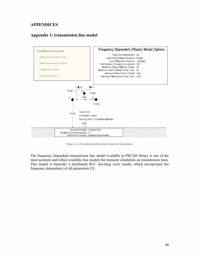
60

APPENDICES

Appendix 1: transmission line model

Figure A.1 Transmission line model used for simulations

The frequency dependent transmission line model available in PSCAD library is one of the most accurate and robust available line models for transient simulation on transmission lines. This model is basically a distributed RLC traveling wave model, which incorporates the frequency dependence of all parameters [5].

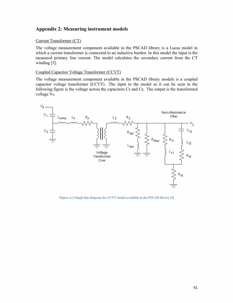
61

Appendix 2: Measuring instrument models

Current Transformer (CT)

The voltage measurement component available in the PSCAD library is a Lucas model in which a current transformer is connected to an inductive burden. In this model the input is the measured primary line current. The model calculates the secondary current from the CT winding [5].

Coupled Capacitor Voltage Transformer (CCVT)

The voltage measurement component available in the PSCAD library models is a coupled capacitor voltage transformer (CCVT). The input to the model as it can be seen in the following figure is the voltage across the capacitors C1 and C2. The output is the transformed voltage VS.

Figure A.2 Single line diagram for CCVT model available in the PSCAD library [5]

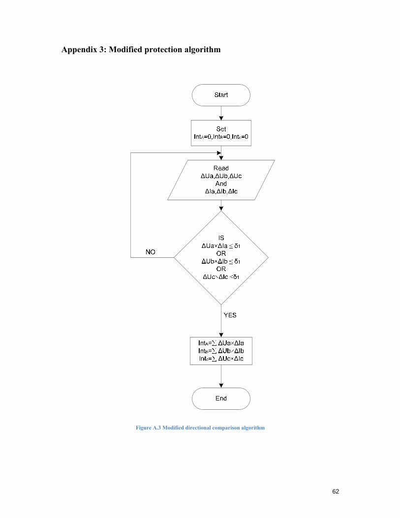
62

Appendix 3: Modified protection algorithm

Figure A.3 Modified directional comparison algorithm

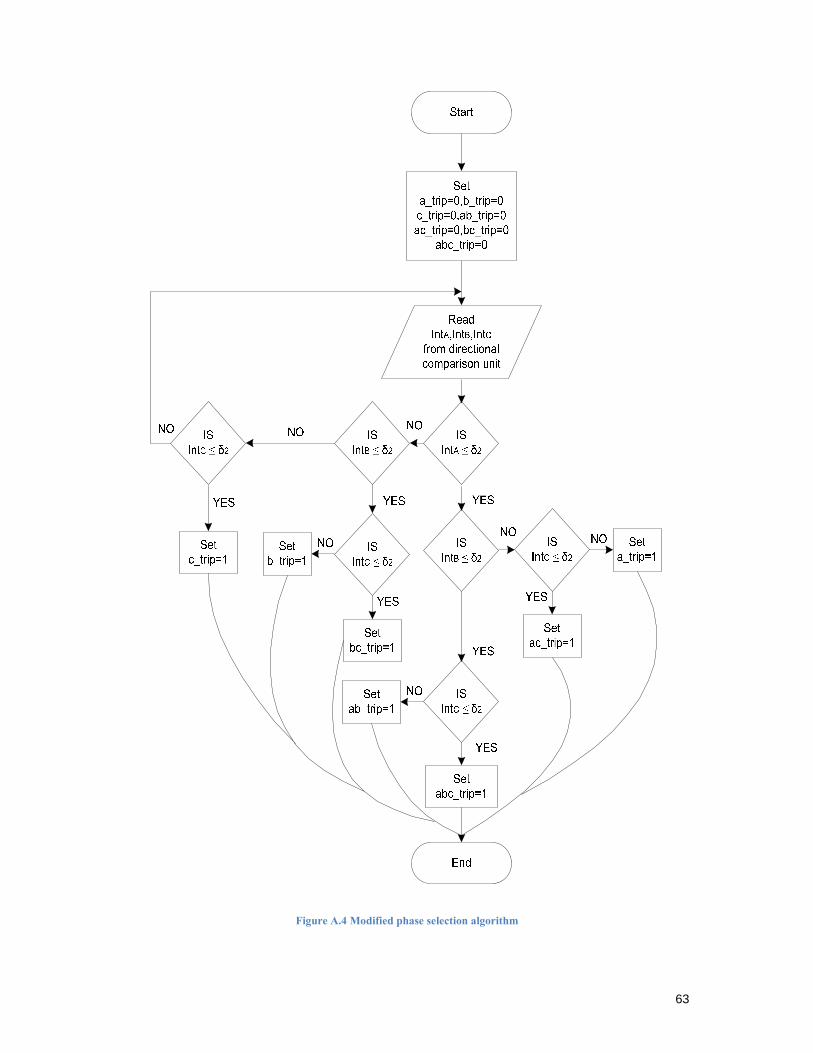
63

Figure A.4 Modified phase selection algorithm

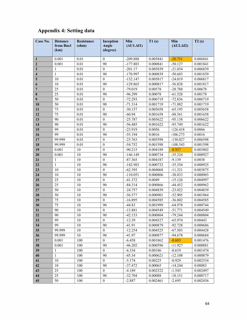
64

Appendix 4: Setting data

Case No.

Distance from Bus1 (km)

Resistance (ohm)

Inception Angle (degree)

Min (ΔU1.ΔI1)

T1 (s)

Min (ΔU2.ΔI2)

T2 (s)

1 0.001 0.01 0 -209.888 0.005841 -20.751 0.006841 2 0.001 0.01 90 -177.883 0.000841 -50.127 0.001841 3 1 0.01 0 -201.17 0.005839 -21.034 0.006839 4 1 0.01 90 -170.997 0.000839 -50.603 0.001839 5 10 0.01 0 -132.147 0.005817 -24.019 0.006817 6 10 0.01 90 -129.865 0.000817 -56.828 0.001817 7 25 0.01 0 -79.019 0.00578 -28.788 0.00678 8 25 0.01 90 -96.299 0.00078 -61.528 0.00178 9 50 0.01 0 -72.293 0.006719 -72.836 0.006719 10 50 0.01 90 -71.314 0.001719 -71.882 0.001719 11 75 0.01 0 -30.157 0.005658 -65.195 0.005658 12 75 0.01 90 -60.94 0.001658 -88.561 0.001658 13 90 0.01 0 -25.787 0.005622 -95.138 0.006622 14 90 0.01 90 -56.485 0.001622 -93.749 0.001622 15 99 0.01 0 -23.919 0.0056 -126.418 0.0066 16 99 0.01 90 -55.194 0.0016 -106.273 0.0016 17 99.999 0.01 0 -23.763 0.005598 -130.027 0.006598 18 99.999 0.01 0 -54.752 0.001598 -108.543 0.001598 19 0.001 10 0 -90.215 0.004189 -8.937 0.003802 20 0.001 10 90 -146.149 0.000734 -35.324 0.000927 21 1 10 0 -87.365 0.004187 -9.139 0.0038 22 1 10 90 -142.983 0.000732 -35.354 0.000925 23 10 10 0 -62.395 0.004068 -11.321 0.003875 24 10 10 90 -110.051 0.000806 -38.033 0.000903 25 25 10 0 -41.372 0.0049 -15.126 0.004997 26 25 10 90 -84.314 0.000866 -44.452 0.000962 27 50 10 0 -24.757 0.004839 -23.022 0.004839 28 50 10 90 -56.577 0.000901 -52.905 0.001964 29 75 10 0 -16.895 0.004585 -36.802 0.004585 30 75 10 90 -44.83 0.001999 -64.978 0.000744 31 90 10 0 -13.881 0.004549 -51.771 0.004549 32 90 10 90 -42.153 0.000804 -79.244 0.000804 33 99 10 0 -12.39 0.004527 -65.974 0.00443 34 99 10 90 -41.91 0.000879 -92.728 0.000686 35 99.999 10 0 -12.254 0.004525 -67.503 0.004428 36 99.999 10 90 -41.97 0.000877 -94.678 0.000684 37 0.001 100 0 -6.458 0.001862 -0.603 0.001476 38 0.001 100 90 -46.202 0.000596 -11.927 0.000881 39 1 100 0 -6.334 0.00186 -0.619 0.001474 40 1 100 90 -45.34 0.000621 -12.108 0.000879 41 10 100 0 -5.174 0.00225 -0.929 0.002534 42 10 100 90 -37.472 0.00065 -14.244 0.00083 43 25 100 0 -4.189 0.002522 -1.545 0.002497 44 25 100 90 -32.704 0.00088 -18.151 0.000717 45 50 100 0 -2.887 0.002461 -2.695 0.002436

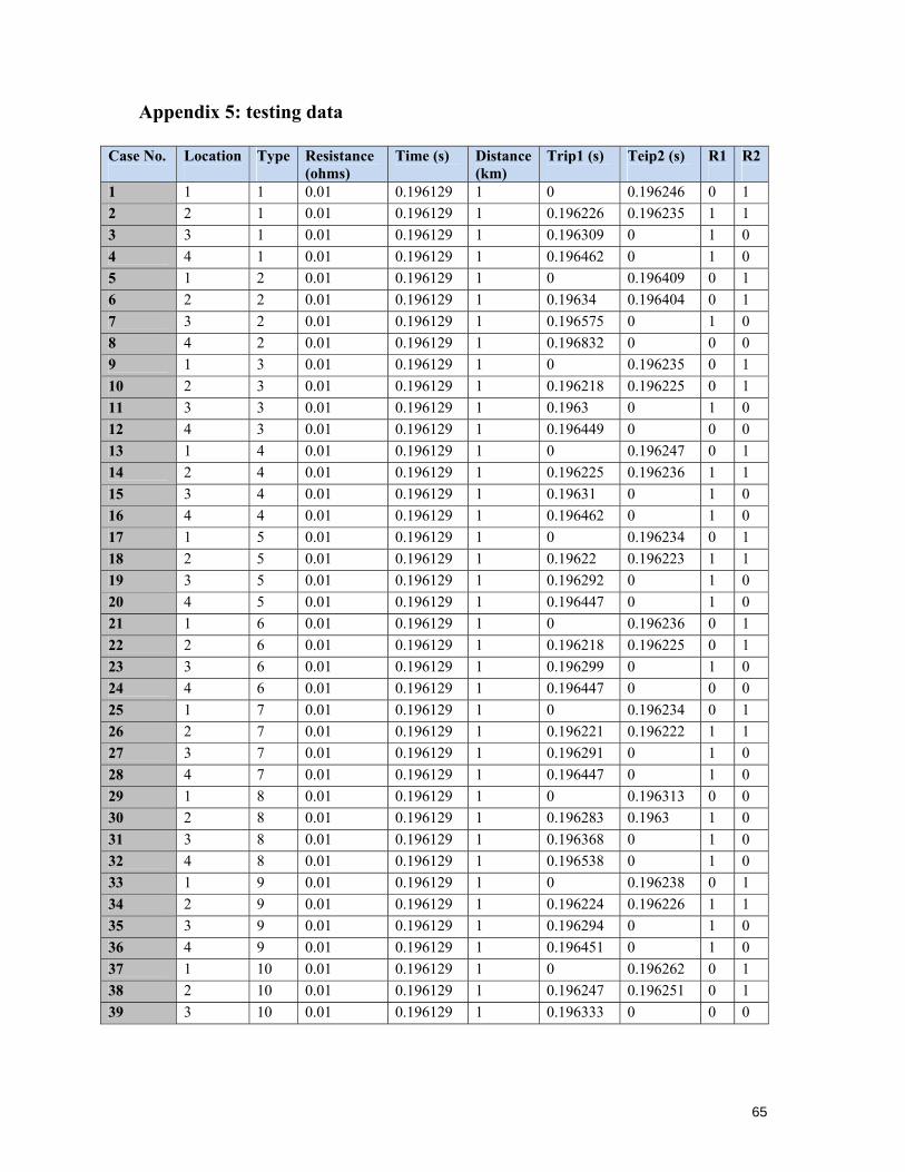
65

Appendix 5: testing data

Case No.

Location

Type

Resistance (ohms)

Time (s)

Distance (km)

Trip1 (s)

Teip2 (s)

R1

R2

1 1 1 0.01 0.196129 1 0 0.196246 0 1 2 2 1 0.01 0.196129 1 0.196226 0.196235 1 1 3 3 1 0.01 0.196129 1 0.196309 0 1 0 4 4 1 0.01 0.196129 1 0.196462 0 1 0 5 1 2 0.01 0.196129 1 0 0.196409 0 1 6 2 2 0.01 0.196129 1 0.19634 0.196404 0 1 7 3 2 0.01 0.196129 1 0.196575 0 1 0 8 4 2 0.01 0.196129 1 0.196832 0 0 0 9 1 3 0.01 0.196129 1 0 0.196235 0 1 10 2 3 0.01 0.196129 1 0.196218 0.196225 0 1 11 3 3 0.01 0.196129 1 0.1963 0 1 0 12 4 3 0.01 0.196129 1 0.196449 0 0 0 13 1 4 0.01 0.196129 1 0 0.196247 0 1 14 2 4 0.01 0.196129 1 0.196225 0.196236 1 1 15 3 4 0.01 0.196129 1 0.19631 0 1 0 16 4 4 0.01 0.196129 1 0.196462 0 1 0 17 1 5 0.01 0.196129 1 0 0.196234 0 1 18 2 5 0.01 0.196129 1 0.19622 0.196223 1 1 19 3 5 0.01 0.196129 1 0.196292 0 1 0 20 4 5 0.01 0.196129 1 0.196447 0 1 0 21 1 6 0.01 0.196129 1 0 0.196236 0 1 22 2 6 0.01 0.196129 1 0.196218 0.196225 0 1 23 3 6 0.01 0.196129 1 0.196299 0 1 0 24 4 6 0.01 0.196129 1 0.196447 0 0 0 25 1 7 0.01 0.196129 1 0 0.196234 0 1 26 2 7 0.01 0.196129 1 0.196221 0.196222 1 1 27 3 7 0.01 0.196129 1 0.196291 0 1 0 28 4 7 0.01 0.196129 1 0.196447 0 1 0 29 1 8 0.01 0.196129 1 0 0.196313 0 0 30 2 8 0.01 0.196129 1 0.196283 0.1963 1 0 31 3 8 0.01 0.196129 1 0.196368 0 1 0 32 4 8 0.01 0.196129 1 0.196538 0 1 0 33 1 9 0.01 0.196129 1 0 0.196238 0 1 34 2 9 0.01 0.196129 1 0.196224 0.196226 1 1 35 3 9 0.01 0.196129 1 0.196294 0 1 0 36 4 9 0.01 0.196129 1 0.196451 0 1 0 37 1 10 0.01 0.196129 1 0 0.196262 0 1 38 2 10 0.01 0.196129 1 0.196247 0.196251 0 1 39 3 10 0.01 0.196129 1 0.196333 0 0 0

66

REFERENCES [1] A. Wright and C. Christopoulos, Electrical Power System Protection, Chapman & Hall, London, U.K, 1993.

[2] Nicholas Villamagna and Peter A.Crossley,“Asymmetrical Component-Based GPS Signal Failure-Detection Algorithm for use in Feeder Current Differential Protection”, IEEE Transaction on power delivery, vol. 23, no. 4, October 2008.

[3] M. Chamia and S. Liberman, “Ultra High Speed Relay for EHV/UHV Transmission Lines Development, Design and Application”, IEEE Transactionson Power Apparatus and Systems, Vol. PAS-97, No. 6, Nov/Dec 1978, pp. 2104-2112.

[4] L.P.Singh, Advanced Power System Analysis and Dynamics, New Age International(P) Limited Publishers, Revised Fourth Edition, India, 2006.

[5] Manitoba HVDC Research Centre, PSCAD/EMTDC User’s Guide, PSCAD V3, Manitoba, 2001.

[6] Areva T&D, Network Protection and Automation Guide (NPAG), 1987.

[7] J. Lewis Blackburn, Protective Relaying, principals and applications, Second Edition, 1997.

[8] IEEE C37.113 Guide for Protective Relay Applications to Transmission Lines

[9] Application guide on protection of complex transmission network configurations: CIGRE materials, CIGRE SC-34 WG 34.04, Nov. 1991.

[10] P.M. Anderson, Power System Protection, McGraw-Hill /IEEE Press, New York, NY, 1999.

[11] Protection using telecommunications: CIGRE materials, CIGRE SC 34/35 JWG 34/35.11, Aug 2001.

[12] A. Apostolov,”Implementation of a Transient Energy Method for Directional Detection in Numerical Distance Relays” IEEE Transmission and Distribution Conference, Volume 1, Issue, 11-16 Apr 1999 Page(s):382 - 387 vol.

[13] Ernesto Vázquez, Jorge Castruita, Oscar L. Chacón, Arturo Conde,“A new Approach Traveling-Wave Distance Protection-Part I:Algorithm”, IEEE TRANSACTIONS ON POWER DELIVERY, VOL. 22, NO. 2, APRIL 2007.

[14] A.P.Sakis Meliopoulos, Power system grounding and transients, Marcel Dekker, Inc, U.S.A, 1988.

[15] L. V. Bewley, Traveling Waves on Transmission Systems, Dover Publications Inc., New York, Second Edition, 1963.

[16] Lanz O E, Engler F, Haenggli M, et al.” LR91— an Ultra-High-Speed Directional Comparison Relay for Protection of High-Voltage Transmission Lines”, BBC Brown Bovril Reviews, 1985, 72 (1):32-36.

[17] Gunnar Nimmersjo,” Arrangement for detecting the direction of a fault from a measuring point”,U.S. Patent No.3,878,460

[18] Application Guide 61-35 AG, ASEA protective relays, type RALDA Directional Wave Relay System, Aug. 1980.

67

[19] Lanz, O.E. Hanggli, M. Bacchini, G. Engler, F. “Transient Signal and Their Processing in An Ultra High-Speed Directional Relay For EHV/UHV Transmission line Protection”, IEEE transactions on power apparatus and systems, PAS-104 June 1985, pp 1463-1473.

[20] M Vitins, “A Fundamental Concept for High Speed Relaying”, Trans IEEE, PAS-100, 1981, pp 163-168.

[21] A T Johns, “New Ultra-High Speed Directional Comparison Technique for the Protection of EHV Transmission Lines”,Proc IEE, Vol 127(c), 1980, pp 228-239.

[22] P.A. Crossley and P.G. McLaren, “Distance Protection Based on Traveling Waves,IEEE Transactions on Power Apparatus and Systems”, Vol. PAS-102, No. 9, September 1983, pp. 2971-2978.

[23] A.T. Johns and S.K. Salman, Digital Protection For Power Systems .United Kingdom: Peter Peregrinus Ltd/ IEE,, 1995.

[24] Power System Protection. Volume 4: Digital Protection and Signaling, The Electricity Training Association, Institution of Electrical Engineers,U.K., 1995.

[25] Abdelsalam Mohamed Elhaffar, “Power transmission line fault location based on current traveling waves”, Doctoral dissertation, Helsinki University of Technology, 2008.

[26] CHUNJU FAN; LI K. K. ; CHAN W. L. ; WEIYONG YU, “Study of protection scheme for transmission line based on wavelet transient energy”, Electrical power & energy systems 2006, vol. 28, no7, pp. 459-470.

[27] Wei Chen; Malik, O.P.; Xianggen Yin; Deshu Chen; Zhe Zhang,”Study of Wavelet-based Ultra High Speed Directional Transmission Line Protection”, IEEE Transactions on Power Delivery Oct. 2003 Page(s): 1134 - 1139

[28] Xinzhou Dong, “Fault Classification and Faulted-Phase Selection Based on the Initial Current Traveling Wave”, IEEE TRANSACTIONS ON POWER DELIVERY, VOL. 24, NO. 2, APRIL 2009.

[29] Xinzhou Dong, Bin Su, Qingping Wang, “Study on the Voltage Traveling Wave wavefront Detection for CVT”, IEEE/PES Transmission and Distribution Conference & Exhibition, Asia and Pacific Dalian, China, 2005.

[30] Xu Bingyin, Shu Zhihuai,Philip Gale,” The Application of Traveling Wave Fault Locators in China”

[31] Z.Q. Bo, F. Jiang, Z.Ched, X.Z. Dong, G.Weller, M.A Redfern,“Transient Based Protection for Power Transmission Systems”, IEEE PES Winter Meeting, Singapore ,Jan 2000.