9TH INTERNATIONAL SYMPOSIUM ON PARTICLE IMAGE VELOCIMETRY – PIV’11 Kobe, Japan, July 21-23, 2011

PIV study of fractal grid turbulence

S. Discetti1, I. B. Ziskin2, R. J. Adrian2, K. Prestridge3

1Dipartimento di Ingegneria Aerospaziale (DIAS), University of Naples Federico II, Naples, Italy stefano.discetti@unina.it

2School for Engineering of Matter, Transport and Energy, Arizona State University,

Tempe, AZ, 85287-6106, USA

3Los Alamos National Laboratory, Los Alamos NM 8754, USA

ABSTRACT The present work describes an experimental investigation of the decay of the wind tunnel turbulence generated by space filling fractal square grids by means of stereoscopic Particle Image Velocimetry (PIV). PIV is severely challenged by measurements of power spectra and measurements of low turbulence intensity flow, and this application involves both. Good statistics require averages over large numbers of frames, and the authors discuss the statistical convergence. Among the quantities to be analysed from the obtained velocity fields are the longitudinal integral length scale, Taylor micro-scale, streamwise two-point correlation functions, and energy spectra. 1. INTRODUCTION Multi-scale generated turbulence has unusual properties that may lead to exciting new insights into turbulence theory as well as important new industrial applications. The study of turbulence generated by fractal elements is motivated by the dissipation anomaly (i.e. the independence of the turbulent kinetic dissipation rate on Reynolds number at high Re), which lies at the root of Kolmogorov’s theory. When turbulence is generated by injecting energy over a range of length scales, as by a fractal grid, the spectral energy transfer mechanism can be investigated by adjusting the geometry of the fractal grid [1]. Hurst and Vassilicos [2] found that space-filling fractal square grids gave the most interesting results, showing an increase of the turbulence intensity until a downstream location xpeak, and a subsequent exponential decay, as opposed to the well-known power law decay of classical square grids [3-4]. During the exponential decay, they found that the ratio of the longitudinal integral length scale L11 to the Taylor microscale λ is nearly constant. Furthermore, Seoud and Vassilicos [5] observed that fractal square grids can generate turbulence of about three times higher Reynolds number Reλ than turbulence generated by classical grids, and comparable to turbulence generated by jet grids [6] and active grids [7] with the same flow speed and significantly lower blockage ratio. All measurements to date have been made using the hot-wire anemometer. The measurement of power spectra and turbulence statistics is, in low turbulence intensity flow, a challenge for PIV. However, up-to-date cameras allow high spatial resolution, enabling the possibility to extract turbulence statistics from the flow field. In the present work we present a Stereo PIV investigation of fractal/multiscale-generated turbulence. In Sec. 2 the geometry of the adopted space-filling fractal grids is presented; in Sec. 3 the experimental setup, and

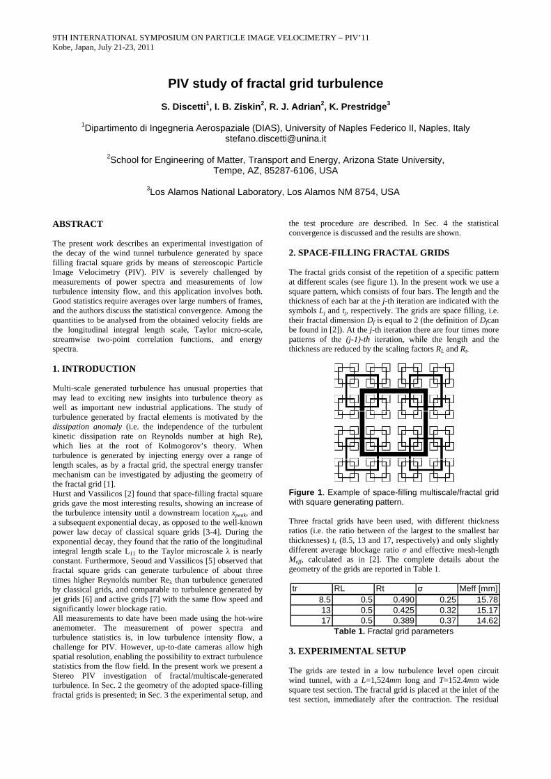
the test procedure are described. In Sec. 4 the statistical convergence is discussed and the results are shown. 2. SPACE-FILLING FRACTAL GRIDS The fractal grids consist of the repetition of a specific pattern at different scales (see figure 1). In the present work we use a square pattern, which consists of four bars. The length and the thickness of each bar at the j-th iteration are indicated with the symbols Lj and tj, respectively. The grids are space filling, i.e. their fractal dimension Df is equal to 2 (the definition of Dfcan be found in [2]). At the j-th iteration there are four times more patterns of the (j-1)-th iteration, while the length and the thickness are reduced by the scaling factors RL and Rt.

Figure 1. Example of space-filling multiscale/fractal grid with square generating pattern.

Three fractal grids have been used, with different thickness ratios (i.e. the ratio between of the largest to the smallest bar thicknesses) tr (8.5, 13 and 17, respectively) and only slightly different average blockage ratio σ and effective mesh-length Meff, calculated as in [2]. The complete details about the geometry of the grids are reported in Table 1.

Table 1. Fractal grid parameters

3. EXPERIMENTAL SETUP The grids are tested in a low turbulence level open circuit wind tunnel, with a L=1,524mm long and T=152.4mm wide square test section. The fractal grid is placed at the inlet of the test section, immediately after the contraction. The residual

tr RL Rt σ Meff [mm]8.5 0.5 0.490 0.25 15.7813 0.5 0.425 0.32 15.1717 0.5 0.389 0.37 14.62

level of turbulence in absence of the grid is lower than 0.5% along the centerline of the wind tunnel. number, based oncontraction without the grids,the fractal grid, ranges between 8on the fractal grid).Seeding, in the form of oil droplets of diameter of approximately 1µm, is injected It is illuminated by a laser light sheet, generated by doublecavity Nd-YAG laser, with a thickness of about 0.5pulse duration of 8maximum energy per pulse of 100The experiments are carried out with an angularstereoscopic PIV configuration, with cameras placed at +40°, 40°. TSI POWERVIEW™ Plus 11MP pixels), equipped w60mm, are employed to record images with about 22 pixels/mm resolutionsatisfied to obtain A grid of dots, with diameter of 0.5has been generated to perform the optical calibration of the system. A translation stage movethe z direction (where the streamwise and crosswise directions in the light sheet plane, and the z axis completes the three dimensional orthogonal reference system pointing towards the cameras) with an accuracy of 13order in x, y, and between world and image coordicorrection between the laser sheet and the performed as proposed by Wieneke [9]. The so called disparity map is computed on 50 samples, and then averaged to suppress the effect of noise.The imaging system is placed in order to investigate the characteristics of the evolution of the generated structures throughout their decay history, and to assess the sensitivity of the measurement setup in detecting the level of turbulence intensity. The displacement fields are obtained by interrogating the two warped images with a standard homebuilt multisoftware with windowthe three-component (3C) displacement field is computed by a procedure including both dewarping and 3C reconstruction, as proposed by Soloff et al. [11]. The final dimension of the interrogation spot is 1650% overlap. The results are averaged over 4. RESULTS 4.1 Instantaneous velocity fieldsIn this section some features of the instantaneous velocity field are briefly illustrated. The flow is characterized by a range of length scales and structures. In figure 2 (top) an example of instantaneous distribution of the is illustrated. The flow field is smoothed by a Gaussian filtering window, with a 3 x 3 kernel and a standard deviation equal to 1. A magnified illustration of the highlighted zone is presented in figure 2, bottom. The vector rvelocity field is also reported. The turbulent structures composed of scales of the order of the Taylor microthe motion are satisfactorily resolved. calculated as described in Sec. 4.4, is i.e. about 3.7 times the linear dimension of the interrogation spot.

level of turbulence in absence of the grid is lower than 0.5% along the centerline of the wind tunnel.

based on the velocity without the grids,

the fractal grid, ranges between 8fractal grid).

Seeding, in the form of oil droplets of diameter of approximately 1µm, is injected t is illuminated by a laser light sheet, generated by double

YAG laser, with a thickness of about 0.5pulse duration of 8ns, a pulse frequency of 2maximum energy per pulse of 100The experiments are carried out with an angularstereoscopic PIV configuration, with cameras placed at +40°,

TSI POWERVIEW™ Plus 11MP pixels), equipped with Nikon objectives with a focal length of

employed to record images with about 22 pixels/mm resolution. The Scheimpflug condition [8] is satisfied to obtain uniform focusing of the images.A grid of dots, with diameter of 0.5has been generated to perform the optical calibration of the system. A translation stage move

direction (where the streamwise and crosswise directions in the light sheet plane,

axis completes the three dimensional orthogonal reference system pointing towards the cameras) with an accuracy of 13µm. Polynomial mapping functions of the third

, and z, are employed to fit the correspondence between world and image coordicorrection between the laser sheet and the performed as proposed by Wieneke [9]. The so called disparity map is computed on 50 samples, and then averaged to suppress the effect of noise.The imaging system is placed in order to investigate the characteristics of the evolution of the generated structures throughout their decay history, and to assess the sensitivity of the measurement setup in detecting the level of turbulence intensity. The displacement fields are obtained by interrogating the two warped images with a standard homebuilt multisoftware with window deformation, as described in [10

component (3C) displacement field is computed by a e including both dewarping and 3C reconstruction, as

proposed by Soloff et al. [11]. The final dimension of the interrogation spot is 16 x 16

lap. The results are averaged over

4. RESULTS

ntaneous velocity fieldsIn this section some features of the instantaneous velocity field are briefly illustrated. The flow is characterized by a range of length scales and structures. In figure 2 (top) an example of instantaneous distribution of the is illustrated. The flow field is smoothed by a Gaussian filtering window, with a 3 x 3 kernel and a standard deviation

A magnified illustration of the highlighted zone is presented in figure 2, bottom. The vector rvelocity field is also reported. The turbulent structures composed of scales of the order of the Taylor microthe motion are satisfactorily resolved. calculated as described in Sec. 4.4, is

3.7 times the linear dimension of the interrogation

level of turbulence in absence of the grid is lower than 0.5% along the centerline of the wind tunnel. The test Reynolds

ocity at the exit section of the without the grids, and the effective mesh

the fractal grid, ranges between 8,500 and 9

Seeding, in the form of oil droplets of diameter of approximately 1µm, is injected uniformly into the fluid flow. t is illuminated by a laser light sheet, generated by double

YAG laser, with a thickness of about 0.5pulse frequency of 2

maximum energy per pulse of 100mJ. The experiments are carried out with an angularstereoscopic PIV configuration, with cameras placed at +40°,

TSI POWERVIEW™ Plus 11MP cameras (4008 x 2672 ith Nikon objectives with a focal length of

employed to record images with about 22 . The Scheimpflug condition [8] is

uniform focusing of the images.A grid of dots, with diameter of 0.5mm and spacing of 5has been generated to perform the optical calibration of the system. A translation stage moves the calibration target along

direction (where the x and y axis coincide with the streamwise and crosswise directions in the light sheet plane,

axis completes the three dimensional orthogonal reference system pointing towards the cameras) with an

. Polynomial mapping functions of the third , are employed to fit the correspondence

between world and image coordinates. The misalignment correction between the laser sheet and the performed as proposed by Wieneke [9]. The so called disparity map is computed on 50 samples, and then averaged to suppress the effect of noise. The imaging system is placed in three streamwise locations, in order to investigate the characteristics of the evolution of the generated structures throughout their decay history, and to assess the sensitivity of the measurement setup in detecting the level of turbulence intensity. The displacement fields are obtained by interrogating the two warped images with a standard homebuilt multi

deformation, as described in [10component (3C) displacement field is computed by a e including both dewarping and 3C reconstruction, as

proposed by Soloff et al. [11]. The final dimension of the 16 pixels = 0.727

lap. The results are averaged over

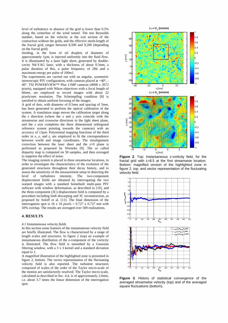
ntaneous velocity fields In this section some features of the instantaneous velocity field are briefly illustrated. The flow is characterized by a range of length scales and structures. In figure 2 (top) an example of instantaneous distribution of the z-component of the vorticity is illustrated. The flow field is smoothed by a Gaussian filtering window, with a 3 x 3 kernel and a standard deviation

A magnified illustration of the highlighted zone is presented in figure 2, bottom. The vector representation of the fluctuating velocity field is also reported. The turbulent structures composed of scales of the order of the Taylor microthe motion are satisfactorily resolved. The Taylor microcalculated as described in Sec. 4.4, is of approximately 2.6

3.7 times the linear dimension of the interrogation

level of turbulence in absence of the grid is lower than 0.5% The test Reynolds

the exit section of the and the effective mesh-length of

500 and 9,200 (depending

Seeding, in the form of oil droplets of diameter of uniformly into the fluid flow.

t is illuminated by a laser light sheet, generated by doubleYAG laser, with a thickness of about 0.5mm

pulse frequency of 2Hz and a

The experiments are carried out with an angular, symmetric stereoscopic PIV configuration, with cameras placed at +40°,

cameras (4008 x 2672 ith Nikon objectives with a focal length of

employed to record images with about 22 . The Scheimpflug condition [8] is

uniform focusing of the images. and spacing of 5mm

has been generated to perform the optical calibration of the the calibration target along

axis coincide with the streamwise and crosswise directions in the light sheet plane,

axis completes the three dimensional orthogonal reference system pointing towards the cameras) with an

. Polynomial mapping functions of the third , are employed to fit the correspondence

The misalignment correction between the laser sheet and the z=0 plane is performed as proposed by Wieneke [9]. The so called disparity map is computed on 50 samples, and then averaged

three streamwise locations, in order to investigate the characteristics of the evolution of the generated structures throughout their decay history, and to assess the sensitivity of the measurement setup in detecting the level of turbulence intensity. The two-component displacement fields are obtained by interrogating the two warped images with a standard homebuilt multi-pass PIV

deformation, as described in [10], and component (3C) displacement field is computed by a e including both dewarping and 3C reconstruction, as

proposed by Soloff et al. [11]. The final dimension of the = 0.727 x 0.727 mm with

500 realizations.

In this section some features of the instantaneous velocity field are briefly illustrated. The flow is characterized by a range of length scales and structures. In figure 2 (top) an example of

component of the vorticity is illustrated. The flow field is smoothed by a Gaussian filtering window, with a 3 x 3 kernel and a standard deviation

A magnified illustration of the highlighted zone is presented in epresentation of the fluctuating

velocity field is also reported. The turbulent structures composed of scales of the order of the Taylor micro-scale of

The Taylor micro-scale, of approximately 2.6mm

3.7 times the linear dimension of the interrogation

level of turbulence in absence of the grid is lower than 0.5% The test Reynolds

the exit section of the length of

,200 (depending

Seeding, in the form of oil droplets of diameter of uniformly into the fluid flow.

t is illuminated by a laser light sheet, generated by double-mm, a and a

symmetric stereoscopic PIV configuration, with cameras placed at +40°, -

cameras (4008 x 2672 ith Nikon objectives with a focal length of

employed to record images with about 22 . The Scheimpflug condition [8] is

mm, has been generated to perform the optical calibration of the

the calibration target along axis coincide with the

streamwise and crosswise directions in the light sheet plane, axis completes the three dimensional orthogonal

reference system pointing towards the cameras) with an . Polynomial mapping functions of the third

, are employed to fit the correspondence The misalignment

plane is performed as proposed by Wieneke [9]. The so called disparity map is computed on 50 samples, and then averaged

three streamwise locations, in order to investigate the characteristics of the evolution of the generated structures throughout their decay history, and to assess the sensitivity of the measurement setup in detecting the

component displacement fields are obtained by interrogating the two

pass PIV ], and

component (3C) displacement field is computed by a e including both dewarping and 3C reconstruction, as

proposed by Soloff et al. [11]. The final dimension of the with

500 realizations.

In this section some features of the instantaneous velocity field are briefly illustrated. The flow is characterized by a range of length scales and structures. In figure 2 (top) an example of

component of the vorticity is illustrated. The flow field is smoothed by a Gaussian filtering window, with a 3 x 3 kernel and a standard deviation

A magnified illustration of the highlighted zone is presented in epresentation of the fluctuating

velocity field is also reported. The turbulent structures scale of

scale, mm,

3.7 times the linear dimension of the interrogation

Figure fractal grid with Bottom: magnified version of the highlighted zone in figure 2, top, and vector representation of the fluctuating velocity field.

Figure averaged streamwise velocity (top) and of the averaged square fluctua

Figure 2. Top: Instantaneous fractal grid with Bottom: magnified version of the highlighted zone in figure 2, top, and vector representation of the fluctuating velocity field.

Figure 3. History of statistical convergence of the averaged streamwise velocity (top) and of the averaged square fluctuations (bottom)

Top: Instantaneous fractal grid with tr=8.5 at the first streamwise locationBottom: magnified version of the highlighted zone in figure 2, top, and vector representation of the fluctuating

History of statistical convergence of the

averaged streamwise velocity (top) and of the averaged tions (bottom).

Top: Instantaneous z-vorticity =8.5 at the first streamwise location

Bottom: magnified version of the highlighted zone in figure 2, top, and vector representation of the fluctuating

History of statistical convergence of the averaged streamwise velocity (top) and of the averaged

field, for the

=8.5 at the first streamwise location.Bottom: magnified version of the highlighted zone in figure 2, top, and vector representation of the fluctuating

History of statistical convergence of the averaged streamwise velocity (top) and of the averaged

field, for the

. Bottom: magnified version of the highlighted zone in figure 2, top, and vector representation of the fluctuating

History of statistical convergence of the averaged streamwise velocity (top) and of the averaged

4.2 Statistical convergenceReliable evaluation of the turbulence statistics requires averaging over a sufficient number of frames. In this section, we discuss the statistical convergence of the results, considering the experiment with theat the first tested streamwise location. The history of convergence is reported the mean squared fluctuations at the location in the centre of the image. The results are normalized by corresponding value averaged over the total number of realizations, wherequantity f averaged over The results show fast convergence of the streamwise velocity (the average varealizations), while the noise effect is much stronger on the mean squared fluctuation (more than 400 samples are needed to reduce the variation below 3%). 4.3 Mean flow featuresIn this section the extracted mean flThe average streamwise velocity component (see figure a jet-like distribution, to the relative low blockage ratio close to the centreline of the wind tunnel. Moving downstream, the homogeneity velocity distribution improvesRegarding the squared fluctuations, the decay along the tunnel centreline is clearly expected, since the streamwise coordinate of the peak of turbulence intensity approximately 29.1, 26.2 and 23.8 mesh lengths for the three fractal grid with thickness ratio equal respectively. The Stereo PIV technique seems to be able to identify the anisotropy of the turbulent fluctuations, as expected [2]. On the other hand, the effect of noise makes it difficult to fit the decay to understand whether it is expFurthermore, the fluctuation of the outcomponent is consistently higher than that of the crosswise velocity component. This effect is due to sensitivity of the stereoscopic reconstruction algorithm in evaluating the outplane displacement, since, for symmetry arguments, the true mean square outnearly equal to the mean square crossfluctuation.

Figure 4. Average streamwise velocity field for the grid tr=8.5, in m/s 4.4 Turbulent statisticsThe measured velocity fields are analysed to extract information about the turbulence statistics. Among the others, the normalized longitudinal two

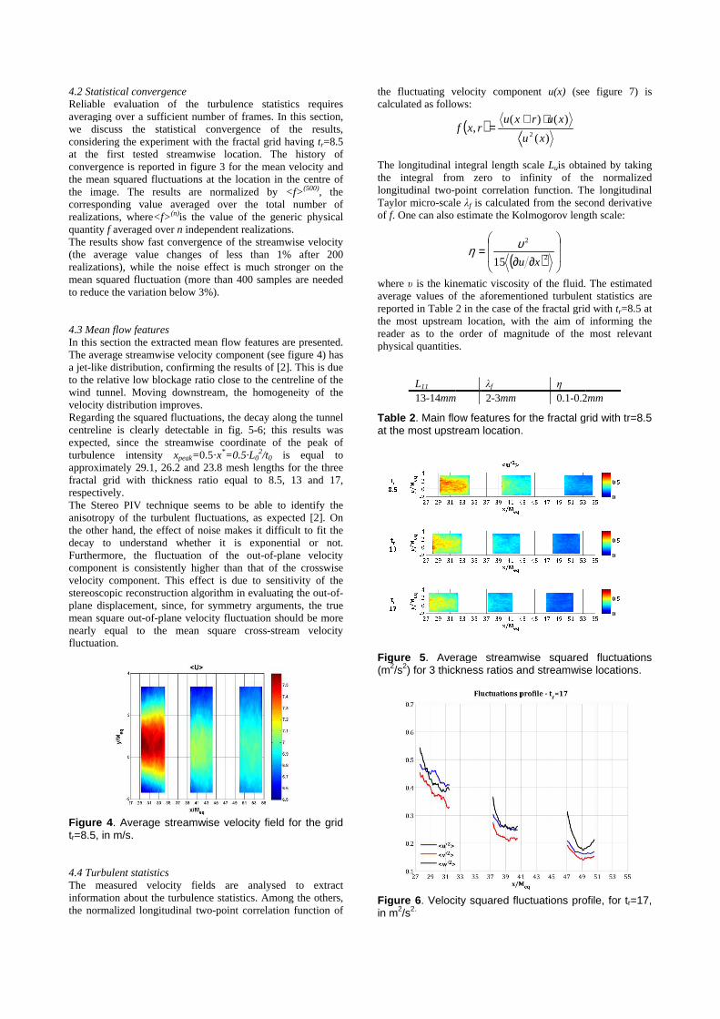
4.2 Statistical convergence Reliable evaluation of the turbulence statistics requires averaging over a sufficient number of frames. In this section,

discuss the statistical convergence of the results, considering the experiment with theat the first tested streamwise location. The history of convergence is reported in figure 3 the mean squared fluctuations at the location in the centre of

The results are normalized by corresponding value averaged over the total number of realizations, where<f> (n)is the value of the generic physical

averaged over n independent realizations.The results show fast convergence of the streamwise velocity (the average value changes of less than 1% after 200 realizations), while the noise effect is much stronger on the mean squared fluctuation (more than 400 samples are needed to reduce the variation below 3%).

4.3 Mean flow features section the extracted mean fl

The average streamwise velocity component (see figure like distribution, confirming the results of

to the relative low blockage ratio close to the centreline of the wind tunnel. Moving downstream, the homogeneity velocity distribution improvesRegarding the squared fluctuations, the decay along the tunnel centreline is clearly detectable in fig. 5expected, since the streamwise coordinate of the peak of turbulence intensity xpeak=approximately 29.1, 26.2 and 23.8 mesh lengths for the three fractal grid with thickness ratio equal

The Stereo PIV technique seems to be able to identify the anisotropy of the turbulent fluctuations, as expected [2]. On the other hand, the effect of noise makes it difficult to fit the decay to understand whether it is expFurthermore, the fluctuation of the outcomponent is consistently higher than that of the crosswise velocity component. This effect is due to sensitivity of the stereoscopic reconstruction algorithm in evaluating the outplane displacement, since, for symmetry arguments, the true mean square out-of-plane velocity fluctuation should be more nearly equal to the mean square cross

Average streamwise velocity field for the grid m/s.

4.4 Turbulent statistics The measured velocity fields are analysed to extract information about the turbulence statistics. Among the others, the normalized longitudinal two

Reliable evaluation of the turbulence statistics requires averaging over a sufficient number of frames. In this section,

discuss the statistical convergence of the results, considering the experiment with the fractal grid having at the first tested streamwise location. The history of

in figure 3 for the mean velocity and the mean squared fluctuations at the location in the centre of

The results are normalized by corresponding value averaged over the total number of

is the value of the generic physical independent realizations.

The results show fast convergence of the streamwise velocity lue changes of less than 1% after 200

realizations), while the noise effect is much stronger on the mean squared fluctuation (more than 400 samples are needed to reduce the variation below 3%).

section the extracted mean flow features are presented. The average streamwise velocity component (see figure

confirming the results ofto the relative low blockage ratio close to the centreline of the wind tunnel. Moving downstream, the homogeneity velocity distribution improves. Regarding the squared fluctuations, the decay along the tunnel

detectable in fig. 5-6; this results was expected, since the streamwise coordinate of the peak of

=0.5·x*=0.5·L02

approximately 29.1, 26.2 and 23.8 mesh lengths for the three fractal grid with thickness ratio equal to 8.5, 13 and 17,

The Stereo PIV technique seems to be able to identify the anisotropy of the turbulent fluctuations, as expected [2]. On the other hand, the effect of noise makes it difficult to fit the decay to understand whether it is expFurthermore, the fluctuation of the outcomponent is consistently higher than that of the crosswise velocity component. This effect is due to sensitivity of the stereoscopic reconstruction algorithm in evaluating the outplane displacement, since, for symmetry arguments, the true

plane velocity fluctuation should be more nearly equal to the mean square cross

Average streamwise velocity field for the grid

The measured velocity fields are analysed to extract information about the turbulence statistics. Among the others, the normalized longitudinal two-point correlation function of

Reliable evaluation of the turbulence statistics requires averaging over a sufficient number of frames. In this section,

discuss the statistical convergence of the results, fractal grid having tr=8.5

at the first tested streamwise location. The history of for the mean velocity and

the mean squared fluctuations at the location in the centre of The results are normalized by <f> (500), the

corresponding value averaged over the total number of is the value of the generic physical independent realizations.

The results show fast convergence of the streamwise velocity lue changes of less than 1% after 200

realizations), while the noise effect is much stronger on the mean squared fluctuation (more than 400 samples are needed

ow features are presented. The average streamwise velocity component (see figure 4) has

confirming the results of [2]. This is due to the relative low blockage ratio close to the centreline of the wind tunnel. Moving downstream, the homogeneity of the

Regarding the squared fluctuations, the decay along the tunnel 6; this results was

expected, since the streamwise coordinate of the peak of 2/t0 is equal to

approximately 29.1, 26.2 and 23.8 mesh lengths for the three to 8.5, 13 and 17,

The Stereo PIV technique seems to be able to identify the anisotropy of the turbulent fluctuations, as expected [2]. On the other hand, the effect of noise makes it difficult to fit the decay to understand whether it is exponential or not. Furthermore, the fluctuation of the out-of-plane velocity component is consistently higher than that of the crosswise velocity component. This effect is due to sensitivity of the stereoscopic reconstruction algorithm in evaluating the outplane displacement, since, for symmetry arguments, the true

plane velocity fluctuation should be more nearly equal to the mean square cross-stream velocity

Average streamwise velocity field for the grid

The measured velocity fields are analysed to extract information about the turbulence statistics. Among the others,

point correlation function of

Reliable evaluation of the turbulence statistics requires averaging over a sufficient number of frames. In this section,

discuss the statistical convergence of the results, =8.5

at the first tested streamwise location. The history of for the mean velocity and

the mean squared fluctuations at the location in the centre of , the

corresponding value averaged over the total number of is the value of the generic physical

The results show fast convergence of the streamwise velocity lue changes of less than 1% after 200

realizations), while the noise effect is much stronger on the mean squared fluctuation (more than 400 samples are needed

ow features are presented. ) has

[2]. This is due to the relative low blockage ratio close to the centreline of the

of the

Regarding the squared fluctuations, the decay along the tunnel 6; this results was

expected, since the streamwise coordinate of the peak of is equal to

approximately 29.1, 26.2 and 23.8 mesh lengths for the three to 8.5, 13 and 17,

The Stereo PIV technique seems to be able to identify the anisotropy of the turbulent fluctuations, as expected [2]. On the other hand, the effect of noise makes it difficult to fit the

onential or not. plane velocity

component is consistently higher than that of the crosswise velocity component. This effect is due to sensitivity of the stereoscopic reconstruction algorithm in evaluating the out-of-plane displacement, since, for symmetry arguments, the true

plane velocity fluctuation should be more stream velocity

Average streamwise velocity field for the grid

The measured velocity fields are analysed to extract information about the turbulence statistics. Among the others,

point correlation function of

the fluctuating velocity component calculated as follows:

The longitudinal integral length scale the integral from zero to infinity of the normalized longitudinal twoTaylor microof f

where average values of the aforementioned turbulent statistics are reported in Table 2 in the casthe most upstream location, with the aim of informing the reader as to the order of magnitude of the most relevant physical quantities.

Table 2at the most upstream location.

Figure (m2

Figure in m

the fluctuating velocity component calculated as follows:

The longitudinal integral length scale the integral from zero to infinity of the normalized longitudinal two-point correlation function. The longitudinal Taylor micro-scale

f. One can also estimate the

where υ is the kinematic viscosity of the fluid. The estimated average values of the aforementioned turbulent statistics are reported in Table 2 in the casthe most upstream location, with the aim of informing the reader as to the order of magnitude of the most relevant physical quantities.

L11

13-14mm

Table 2. Main flow features for the fractal grid with at the most upstream location.

Figure 5. Average streamwise squared fluctuations 2/s2) for 3 thickness ratios and streamwise locations

Figure 6. Velocity squared fluctuations profile, for m2/s2.

f

the fluctuating velocity component calculated as follows:

The longitudinal integral length scale the integral from zero to infinity of the normalized

point correlation function. The longitudinal scale λf is calculated from the second derivative

. One can also estimate the Kolmogorov length scale

is the kinematic viscosity of the fluid. The estimated average values of the aforementioned turbulent statistics are reported in Table 2 in the case of the fractal grid with the most upstream location, with the aim of informing the reader as to the order of magnitude of the most relevant physical quantities.

λf

mm 2-3mm

. Main flow features for the fractal grid with at the most upstream location.

. Average streamwise squared fluctuations thickness ratios and streamwise locations

Velocity squared fluctuations profile, for

( ) (,

xurxf =

(

∂=

15 u

υη

the fluctuating velocity component u(x) (see figure 7)

The longitudinal integral length scale Luis obtained by taking the integral from zero to infinity of the normalized

point correlation function. The longitudinal is calculated from the second derivative

Kolmogorov length scale

is the kinematic viscosity of the fluid. The estimated average values of the aforementioned turbulent statistics are

e of the fractal grid with the most upstream location, with the aim of informing the reader as to the order of magnitude of the most relevant

η 0.1-0.2

. Main flow features for the fractal grid with at the most upstream location.

. Average streamwise squared fluctuations thickness ratios and streamwise locations

Velocity squared fluctuations profile, for

)(

)()2 xu

xur ⋅+

)

∂ 2

2

xu

υ

(see figure 7) is

is obtained by taking the integral from zero to infinity of the normalized

point correlation function. The longitudinal is calculated from the second derivative

Kolmogorov length scale:

is the kinematic viscosity of the fluid. The estimated average values of the aforementioned turbulent statistics are

e of the fractal grid with tr=8.5 at the most upstream location, with the aim of informing the reader as to the order of magnitude of the most relevant

0.2mm

. Main flow features for the fractal grid with tr=8.5

. Average streamwise squared fluctuations thickness ratios and streamwise locations.

Velocity squared fluctuations profile, for tr=17,

is

is obtained by taking the integral from zero to infinity of the normalized

point correlation function. The longitudinal is calculated from the second derivative

is the kinematic viscosity of the fluid. The estimated average values of the aforementioned turbulent statistics are

=8.5 at the most upstream location, with the aim of informing the reader as to the order of magnitude of the most relevant

=8.5

. Average streamwise squared fluctuations

=17,

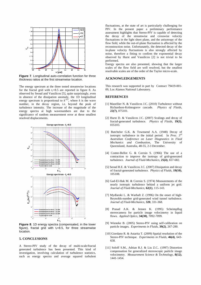
Figure 7. Longitudinal auto-correlation function for three thickness ratios at the first streamwise location. The energy spectrum at the three tested streamwise locations for the fractal grid with tr=8.5 are reported in figure 8. As observed by Seoud and Vassilicos [5], quite surprisingly, even in absence of the dissipation anomaly, the 1D longitudinal energy spectrum is proportional to k-5/3, where k is the wave number, in the decay region, i.e. beyond the peak of turbulence intensity. The increase of the magnitude of the energy spectra at high wavenumbers are due to the significance of random measurement error at these smallest resolved displacements.

Figure 8. 1D energy spectra (compensated, in the lower figure), fractal grid with tr=8.5, for three streamwise location.

5. CONCLUSIONS A Stereo-PIV study of the decay of multi-scale/fractal generated turbulence has been presented. This kind of investigation, involving calculation of turbulence statistics, such as energy spectra and average squared turbulent

fluctuations, at the state of art is particularly challenging for PIV. In the present paper a preliminary performance assessment highlights that Stereo-PIV is capable of detecting the decay of the streamwise and crosswise velocity fluctuations in the light sheet plane, and the anisotropy of the flow field, while the out-of-plane fluctuation is affected by the reconstruction noise. Unfortunately, the detected decay of the in-plane velocity fluctuations is also strongly affected by noise, therefore a fitting to confirm the exponential decay observed by Hurst and Vassilicos [2] is not trivial to be performed. Energy spectra are also presented, showing that the larger scales of the flow field are well resolved, but the smallest resolvable scales are of the order of the Taylor micro-scale. ACKNOWLEDGEMENTS This research was supported in part by Contract 79419-001-09, Los Alamos National Laboratory. REFERENCES [1] Mazellier N. & Vassilicos J.C. (2010) Turbulence without

Richardson-Kolmogorov cascade. Physics of Fluids, 22(7), 075101.

[2] Hurst D. & Vassilicos J.C. (2007) Scalings and decay of

fractal-generated turbulence. Physics of Fluids, 19(3), 035103.

[3] Batchelor G.K. & Townsend A.A. (1948) Decay of

isotropic turbulence in the initial period. In Proc. 3rd Australian Conference on Laser Diagnostics in Fluid Mechanics and Combustion, The University of Queensland, Australia, 48-55, 2-3 December.

[4] Comte-Bellot G. & Corrsin S. (1966) The use of a

contraction to improve the isotropy of grid-generated turbulence. Journal of Fluid-Mechanics, 25(4), 657-682.

[5] Seoud R.E. & Vassilicos J.C. (2007) Dissipation and decay

of fractal-generated turbulence. Physics of Fluids, 19(10), 105108.

[6] Gad-El-Hak M. & Corrsin S. (1974) Measurements of the

nearly isotropic turbulence behind a uniform jet grid. Journal of Fluid-Mechanics, 62(1), 115-143.

[7] Mydlarski L. & Warhaft Z. (1996) On the onset of high-

Reynolds-number grid-generated wind tunnel turbulence. Journal of Fluid-Mechanics, 320, 331-368.

[8] Prasad A.K. & Jensen K. (1995) Scheimpflug

stereocamera for particle image velocimetry in liquid flows. Applied Optics, 34(30), 7092-7099.

[9] Wieneke B. (2005) Stereo-PIV using self-calibration on

particle images. Experiments in Fluids, 39(2), 267-280. [10] Giordano R. & Astarita T. (2009) Spatial resolution of the

Stereo-PIV technique. Experiments in Fluids, 46(4), 643-658.

[11] Soloff S.M., Adrian R.J. & Liu Z.C.. (1997) Distortion

compensation for generalized stereoscopic particle image velocimetry. Measurement Science & Technology, 8(12), 1441-1454.