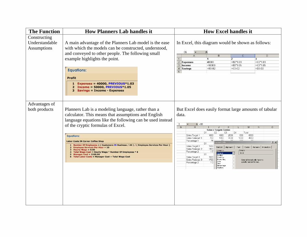
The Function How Planners Lab handles it How Excel handles it Constructing Understandable Assumptions

A main advantage of the Planners Lab model is the ease with which the models can be constructed, understood, and conveyed to other people. The following small example highlights the point.

In Excel, this diagram would be shown as follows:

Advantages of both products

Planners Lab is a modeling language, rather than a calculator. This means that assumptions and English language equations like the following can be used instead of the cryptic formulas of Excel.

But Excel does easily format large amounts of tabular data.

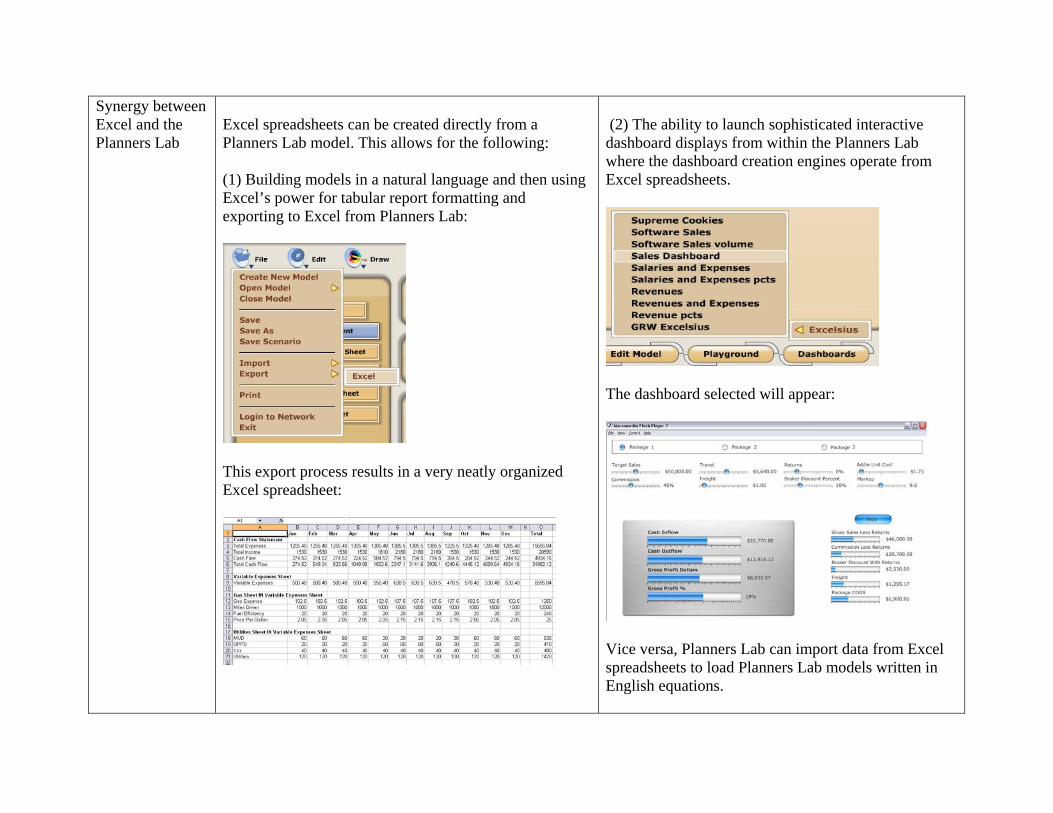
Synergy between Excel and the Planners Lab

Excel spreadsheets can be created directly from a Planners Lab model. This allows for the following: (1) Building models in a natural language and then using Excel’s power for tabular report formatting and exporting to Excel from Planners Lab:

This export process results in a very neatly organized Excel spreadsheet:

(2) The ability to launch sophisticated interactive dashboard displays from within the Planners Lab where the dashboard creation engines operate from Excel spreadsheets.

The dashboard selected will appear:

Vice versa, Planners Lab can import data from Excel spreadsheets to load Planners Lab models written in English equations.

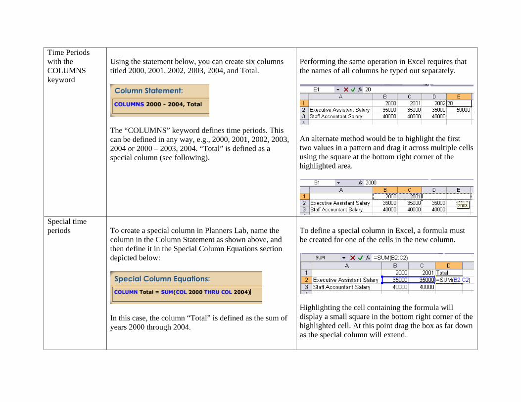
Time Periods with the COLUMNS keyword

Using the statement below, you can create six columns titled 2000, 2001, 2002, 2003, 2004, and Total.

The “COLUMNS” keyword defines time periods. This can be defined in any way, e.g., 2000, 2001, 2002, 2003, 2004 or 2000 – 2003, 2004. “Total” is defined as a special column (see following).

Performing the same operation in Excel requires that the names of all columns be typed out separately.

An alternate method would be to highlight the first two values in a pattern and drag it across multiple cells using the square at the bottom right corner of the highlighted area.

Special time periods

To create a special column in Planners Lab, name the column in the Column Statement as shown above, and then define it in the Special Column Equations section depicted below:

In this case, the column “Total” is defined as the sum of years 2000 through 2004.

To define a special column in Excel, a formula must be created for one of the cells in the new column.

Highlighting the cell containing the formula will display a small square in the bottom right corner of the highlighted cell. At this point drag the box as far down as the special column will extend.

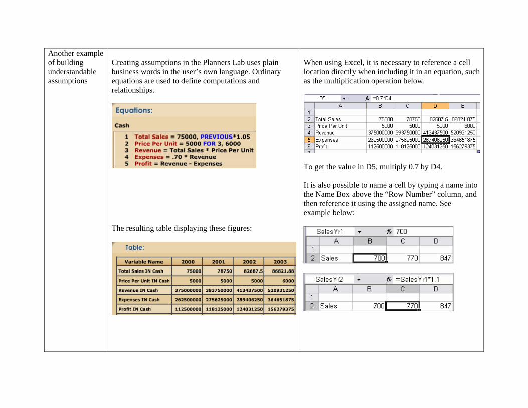
Another example of building understandable assumptions

Creating assumptions in the Planners Lab uses plain business words in the user’s own language. Ordinary equations are used to define computations and relationships.

The resulting table displaying these figures:

When using Excel, it is necessary to reference a cell location directly when including it in an equation, such as the multiplication operation below.

To get the value in D5, multiply 0.7 by D4. It is also possible to name a cell by typing a name into the Name Box above the “Row Number” column, and then reference it using the assigned name. See example below:

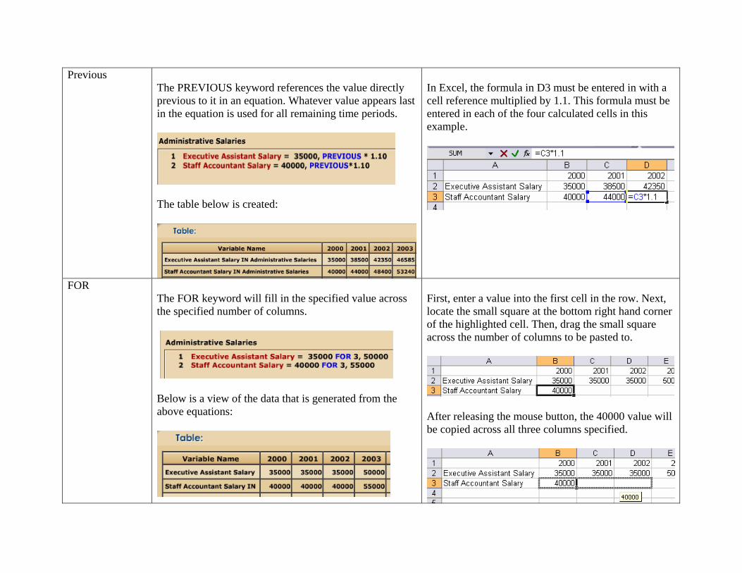
Previous The PREVIOUS keyword references the value directly previous to it in an equation. Whatever value appears last in the equation is used for all remaining time periods.

The table below is created:

In Excel, the formula in D3 must be entered in with a cell reference multiplied by 1.1. This formula must be entered in each of the four calculated cells in this example.

FOR The FOR keyword will fill in the specified value across the specified number of columns.

Below is a view of the data that is generated from the above equations:

First, enter a value into the first cell in the row. Next, locate the small square at the bottom right hand corner of the highlighted cell. Then, drag the small square across the number of columns to be pasted to.

After releasing the mouse button, the 40000 value will be copied across all three columns specified.

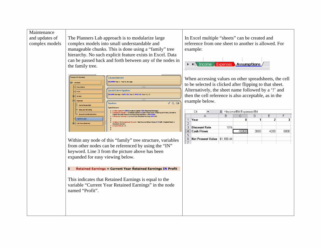
Maintenance and updates of complex models

The Planners Lab approach is to modularize large complex models into small understandable and manageable chunks. This is done using a “family” tree hierarchy. No such explicit feature exists in Excel. Data can be passed back and forth between any of the nodes in the family tree.

Within any node of this “family” tree structure, variables from other nodes can be referenced by using the “IN” keyword. Line 3 from the picture above has been expanded for easy viewing below.

This indicates that Retained Earnings is equal to the variable “Current Year Retained Earnings” in the node named “Profit”.

In Excel multiple “sheets” can be created and reference from one sheet to another is allowed. For example:

When accessing values on other spreadsheets, the cell to be selected is clicked after flipping to that sheet. Alternatively, the sheet name followed by a ‘!’ and then the cell reference is also acceptable, as in the example below.

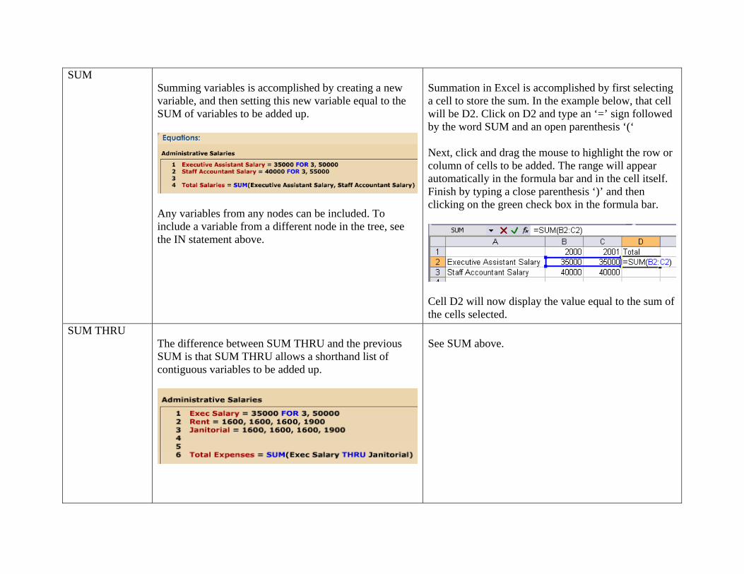
SUM Summing variables is accomplished by creating a new variable, and then setting this new variable equal to the SUM of variables to be added up.

Any variables from any nodes can be included. To include a variable from a different node in the tree, see the IN statement above.

Summation in Excel is accomplished by first selecting a cell to store the sum. In the example below, that cell will be D2. Click on D2 and type an ‘=’ sign followed by the word SUM and an open parenthesis ‘(‘ Next, click and drag the mouse to highlight the row or column of cells to be added. The range will appear automatically in the formula bar and in the cell itself. Finish by typing a close parenthesis ‘)’ and then clicking on the green check box in the formula bar.

Cell D2 will now display the value equal to the sum of the cells selected.

SUM THRU The difference between SUM THRU and the previous SUM is that SUM THRU allows a shorthand list of contiguous variables to be added up.

See SUM above.

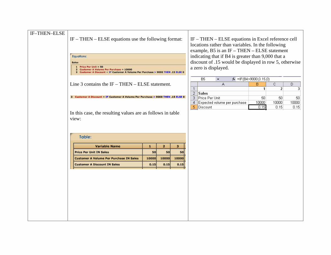
IF–THEN–ELSE IF – THEN – ELSE equations use the following format:

Line 3 contains the IF – THEN – ELSE statement.

In this case, the resulting values are as follows in table view:

IF – THEN – ELSE equations in Excel reference cell locations rather than variables. In the following example, B5 is an IF – THEN – ELSE statement indicating that if B4 is greater than 9,000 that a discount of .15 would be displayed in row 5, otherwise a zero is displayed.

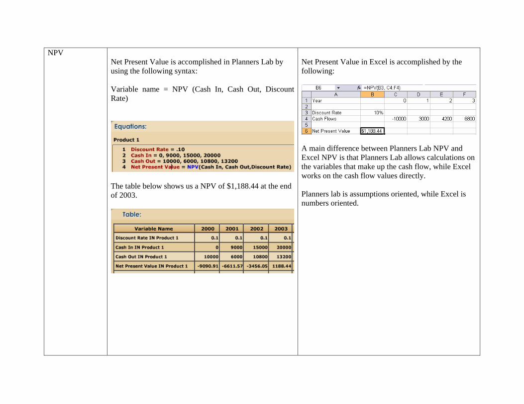
NPV Net Present Value is accomplished in Planners Lab by using the following syntax: Variable name = NPV (Cash In, Cash Out, Discount Rate)

The table below shows us a NPV of $1,188.44 at the end of 2003.

Net Present Value in Excel is accomplished by the following:

A main difference between Planners Lab NPV and Excel NPV is that Planners Lab allows calculations on the variables that make up the cash flow, while Excel works on the cash flow values directly. Planners lab is assumptions oriented, while Excel is numbers oriented.

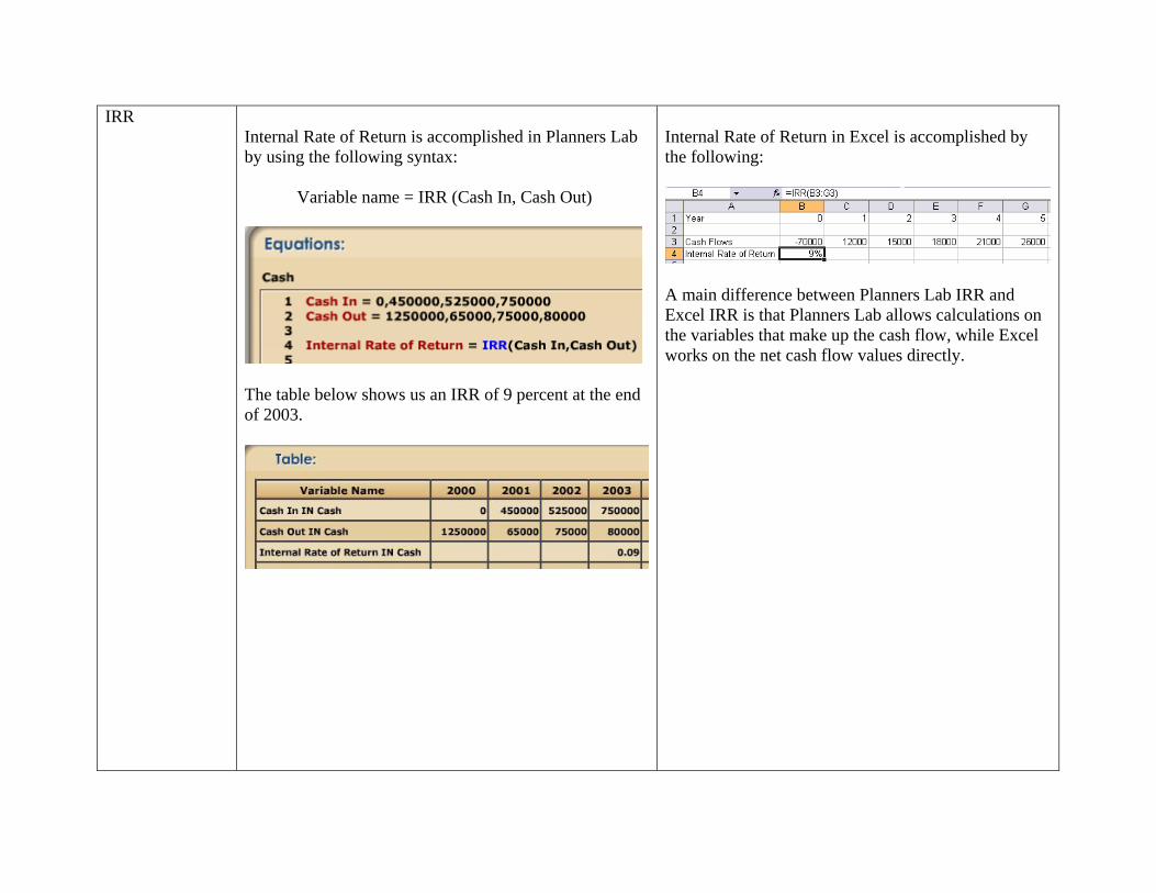
IRR Internal Rate of Return is accomplished in Planners Lab by using the following syntax:

Variable name = IRR (Cash In, Cash Out)

The table below shows us an IRR of 9 percent at the end of 2003.

Internal Rate of Return in Excel is accomplished by the following:

A main difference between Planners Lab IRR and Excel IRR is that Planners Lab allows calculations on the variables that make up the cash flow, while Excel works on the net cash flow values directly.

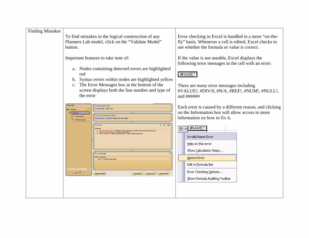
Finding Mistakes To find mistakes in the logical construction of any Planners Lab model, click on the “Validate Model” button. Important features to take note of:

a. Nodes containing detected errors are highlighted red

b. Syntax errors within nodes are highlighted yellow c. The Error Messages box at the bottom of the

screen displays both the line number and type of the error

Error checking in Excel is handled in a more “on-the-fly” basis. Whenever a cell is edited, Excel checks to see whether the formula or value is correct. If the value is not useable, Excel displays the following error messages in the cell with an error:

There are many error messages including #VALUE!, #DIV/0, #N/A, #REF!, #NUM!, #NULL!, and ###### Each error is caused by a different reason, and clicking on the Information box will allow access to more information on how to fix it.

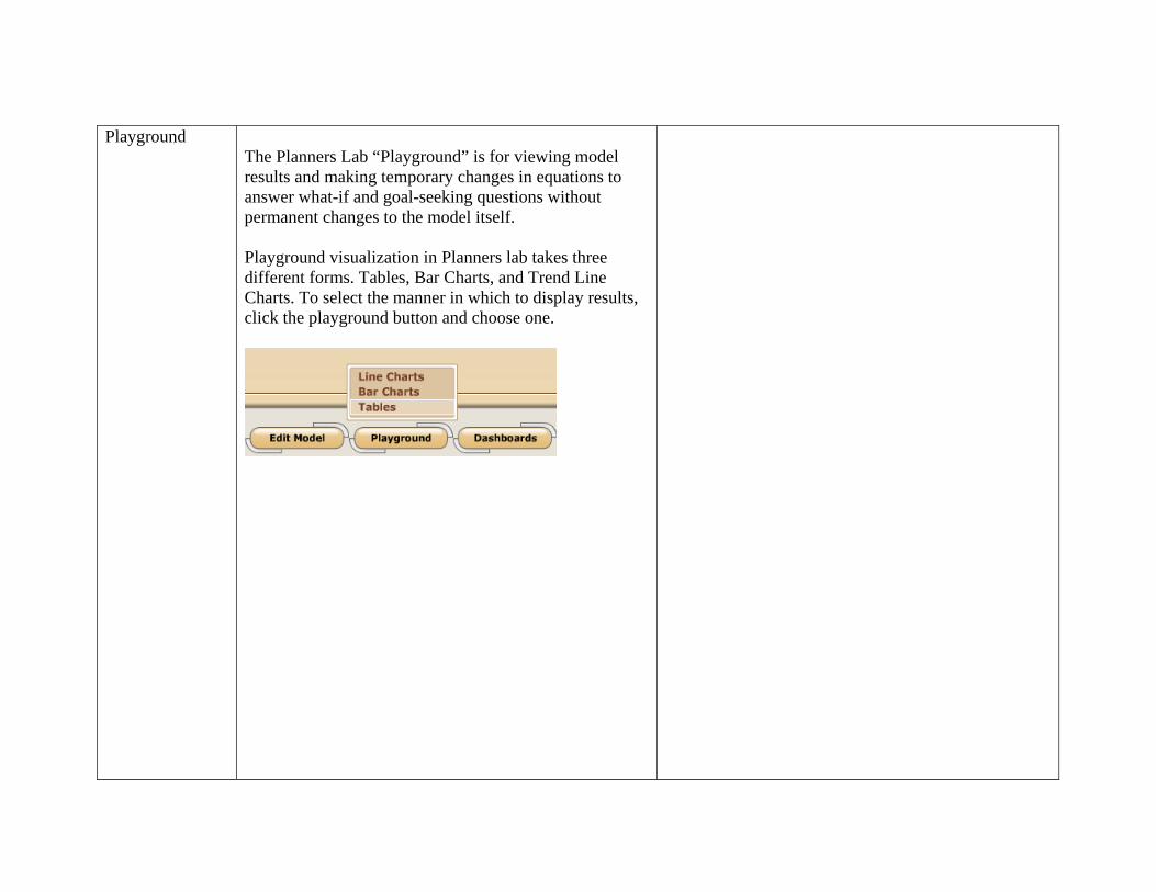
Playground

The Planners Lab “Playground” is for viewing model results and making temporary changes in equations to answer what-if and goal-seeking questions without permanent changes to the model itself. Playground visualization in Planners lab takes three different forms. Tables, Bar Charts, and Trend Line Charts. To select the manner in which to display results, click the playground button and choose one.

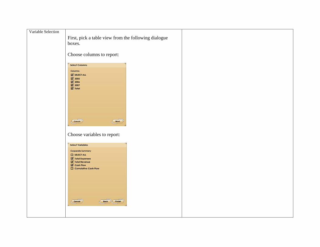
Variable Selection

First, pick a table view from the following dialogue boxes. Choose columns to report:

Choose variables to report:

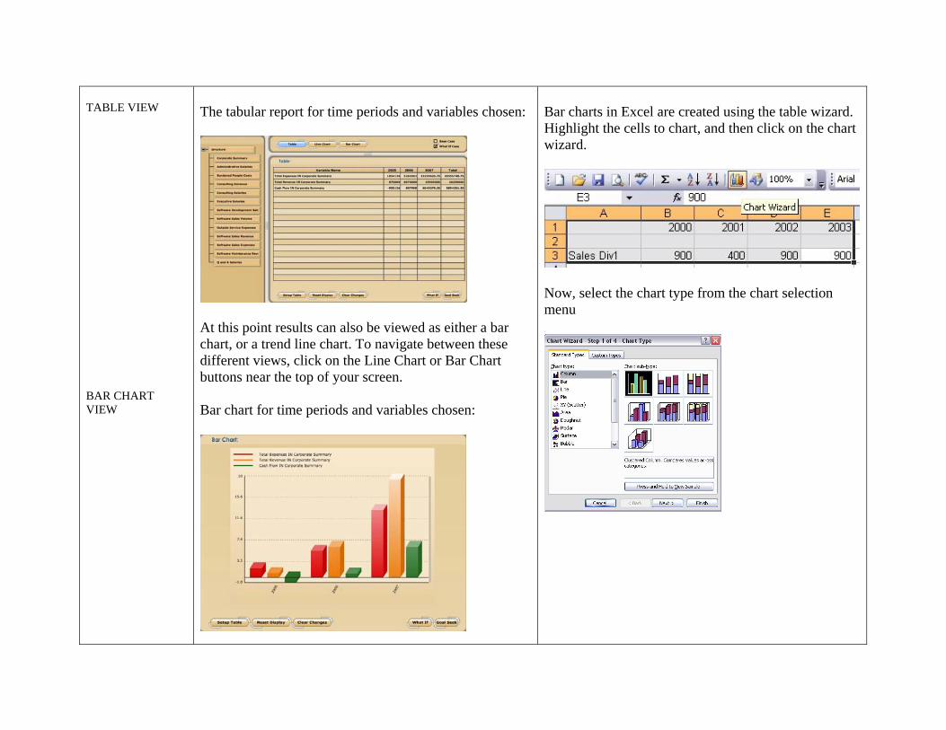
TABLE VIEW BAR CHART VIEW

The tabular report for time periods and variables chosen:

At this point results can also be viewed as either a bar chart, or a trend line chart. To navigate between these different views, click on the Line Chart or Bar Chart buttons near the top of your screen. Bar chart for time periods and variables chosen:

Bar charts in Excel are created using the table wizard. Highlight the cells to chart, and then click on the chart wizard.

Now, select the chart type from the chart selection menu

LINE CHART VIEW What-If and Goal Seek analysis with the Table option

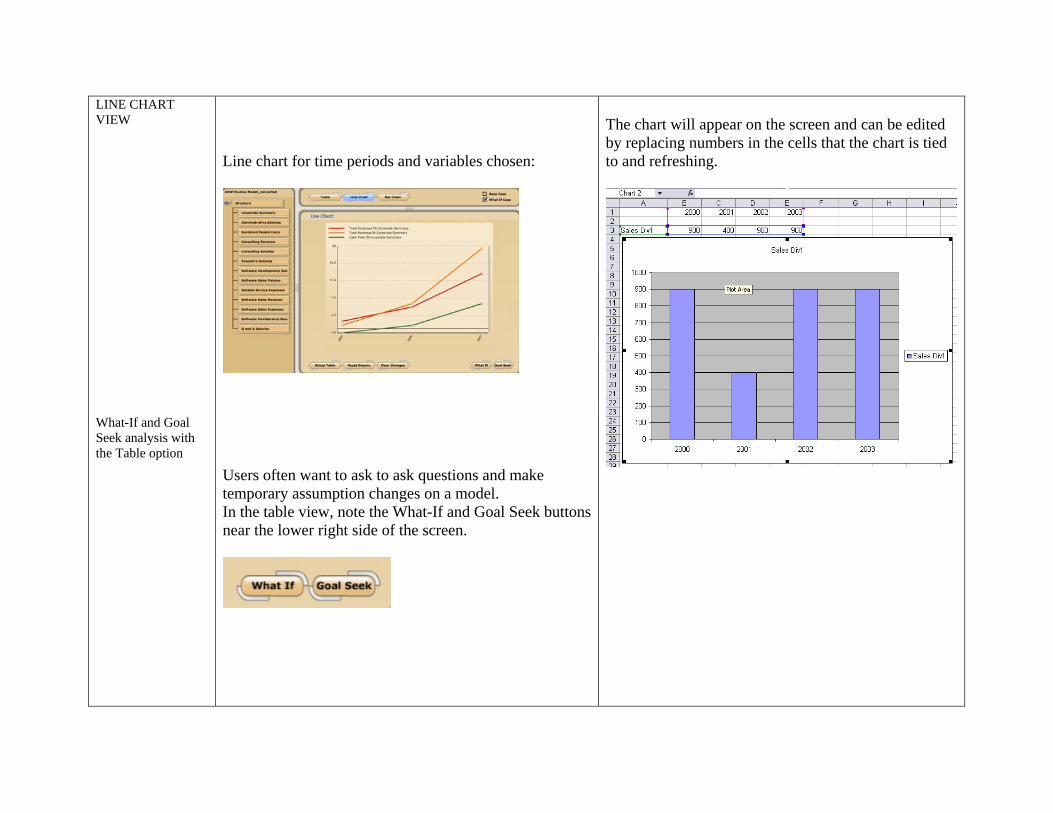
Line chart for time periods and variables chosen:

Users often want to ask to ask questions and make temporary assumption changes on a model. In the table view, note the What-If and Goal Seek buttons near the lower right side of the screen.

The chart will appear on the screen and can be edited by replacing numbers in the cells that the chart is tied to and refreshing.

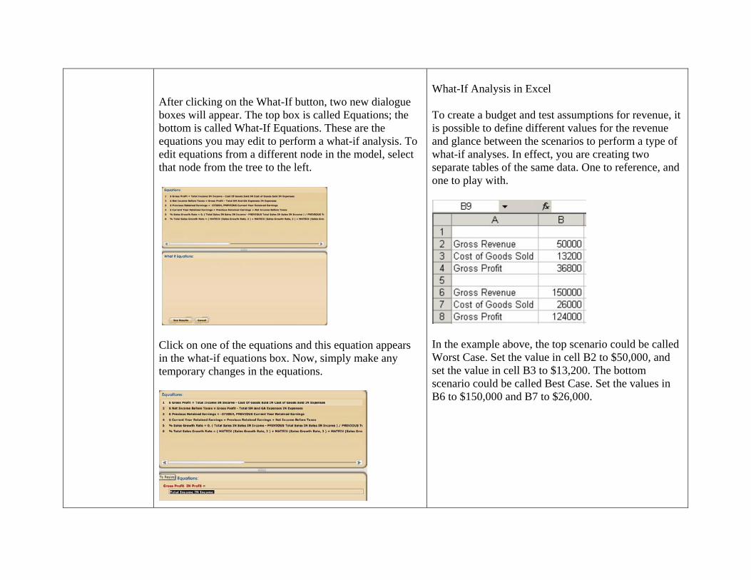
After clicking on the What-If button, two new dialogue boxes will appear. The top box is called Equations; the bottom is called What-If Equations. These are the equations you may edit to perform a what-if analysis. To edit equations from a different node in the model, select that node from the tree to the left.

Click on one of the equations and this equation appears in the what-if equations box. Now, simply make any temporary changes in the equations.

What-If Analysis in Excel To create a budget and test assumptions for revenue, it is possible to define different values for the revenue and glance between the scenarios to perform a type of what-if analyses. In effect, you are creating two separate tables of the same data. One to reference, and one to play with.

In the example above, the top scenario could be called Worst Case. Set the value in cell B2 to $50,000, and set the value in cell B3 to $13,200. The bottom scenario could be called Best Case. Set the values in B6 to $150,000 and B7 to $26,000.

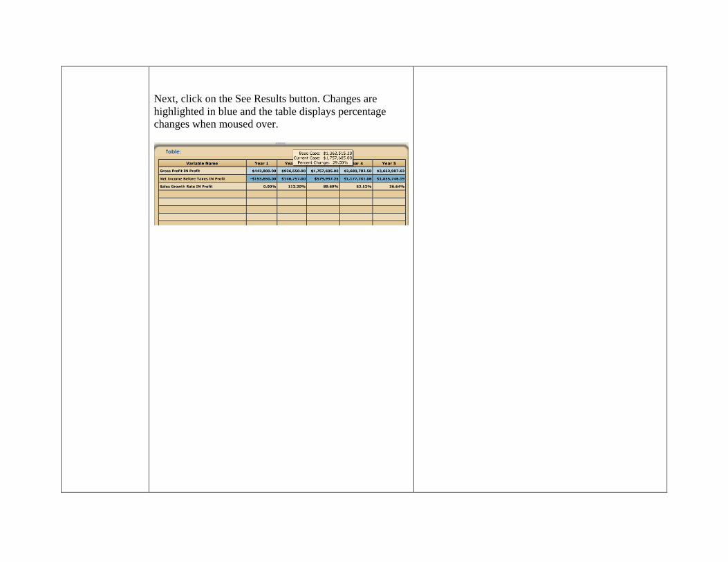
Next, click on the See Results button. Changes are highlighted in blue and the table displays percentage changes when moused over.

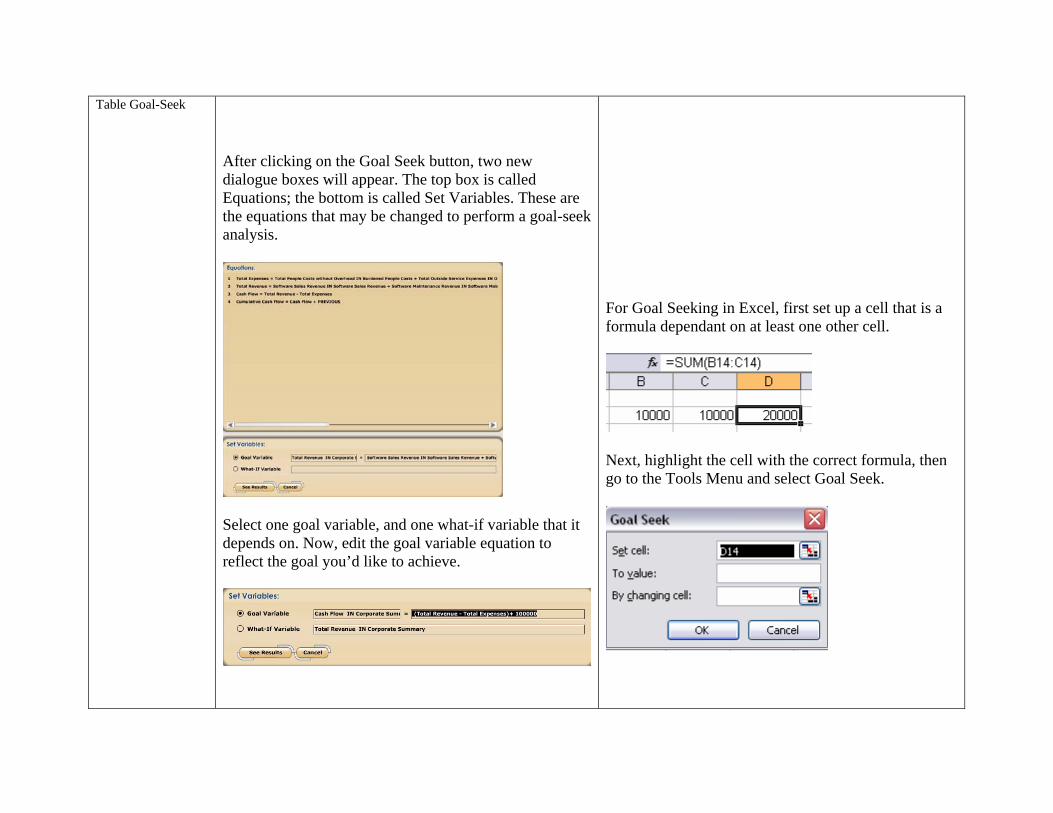
Table Goal-Seek

After clicking on the Goal Seek button, two new dialogue boxes will appear. The top box is called Equations; the bottom is called Set Variables. These are the equations that may be changed to perform a goal-seek analysis.

Select one goal variable, and one what-if variable that it depends on. Now, edit the goal variable equation to reflect the goal you’d like to achieve.

For Goal Seeking in Excel, first set up a cell that is a formula dependant on at least one other cell.

Next, highlight the cell with the correct formula, then go to the Tools Menu and select Goal Seek.

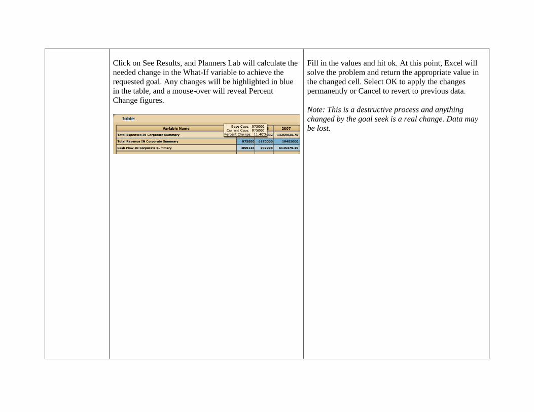
Click on See Results, and Planners Lab will calculate the needed change in the What-If variable to achieve the requested goal. Any changes will be highlighted in blue in the table, and a mouse-over will reveal Percent Change figures.

Fill in the values and hit ok. At this point, Excel will solve the problem and return the appropriate value in the changed cell. Select OK to apply the changes permanently or Cancel to revert to previous data. Note: This is a destructive process and anything changed by the goal seek is a real change. Data may be lost.

Draggable Bar Chart option in the Playground

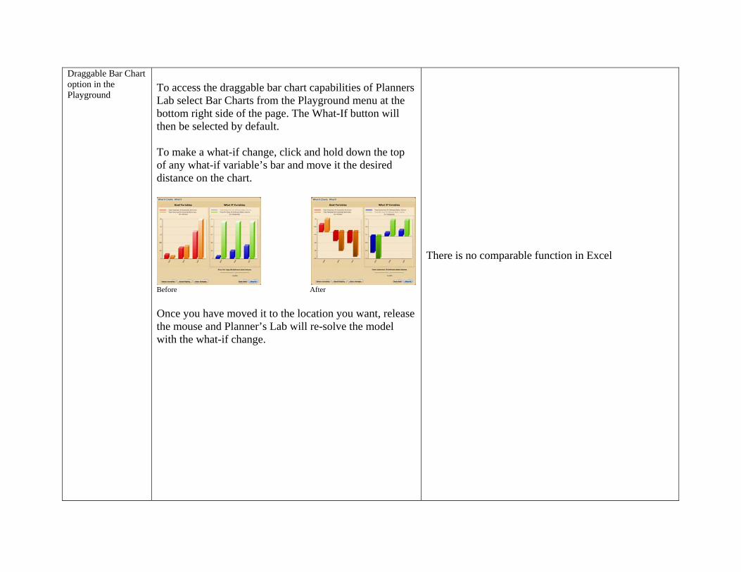
To access the draggable bar chart capabilities of Planners Lab select Bar Charts from the Playground menu at the bottom right side of the page. The What-If button will then be selected by default. To make a what-if change, click and hold down the top of any what-if variable’s bar and move it the desired distance on the chart.

Before After Once you have moved it to the location you want, release the mouse and Planner’s Lab will re-solve the model with the what-if change.

There is no comparable function in Excel

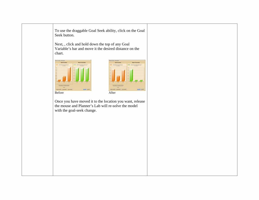
To use the draggable Goal Seek ability, click on the Goal Seek button. Next, , click and hold down the top of any Goal Variable’s bar and move it the desired distance on the chart.

Before After Once you have moved it to the location you want, release the mouse and Planner’s Lab will re-solve the model with the goal-seek change.

Draggable Trend Line Chart option for What-If

To access the draggable trend line charting capabilities of Planners Lab select Trend Line Charts from the Playground menu. To make a what-if change, click and hold down any part of a what-if variable’s line and move it to the desired point Dragging the line in between points will move the entire line.

Before After Once the line or node is in the desired position, release the mouse and Planner’s Lab will re-solve the model with your new what-if change. The base quantity is reflected by a dashed line.

There is no comparable function in Excel.

Draggable Trend Line option for Goal Seek

To make a goal-seek change to the line chart, click on the goal seek button. Next, click and hold down any part on any goal seek variable’s line and move it to the desired point. In this format, only one goal variable and one what-if variable are selectable. However, you may switch between what-if variables by clicking on the charts to the right, and between goal variables by clicking on the names above the Goal Variables chart.

Before After Once the line or node is in the desired position, release the mouse and Planner’s Lab will re-solve the model with your new goal-seek change. The base quantity is reflected by a dashed line.