PLP 6404

Epidemiology of Plant Diseases

Spring 2015

Ariena van Bruggen, modified from Katherine Stevenson

Lecture 18: Disease progress in space: analysis of spatial pattern

Spatial pattern in plant pathology:

the arrangement of diseased entities relative to each other and to the architecture of the

host crop

Why is spatial pattern important to consider?

Provides insight into the spatial characteristics of epidemics

Allows development of plausible biological and environmental hypotheses to

account for the associations among pathogen propagules or diseased plants

Adds an important dimension to temporal analysis of epidemics

Essential for designing sampling protocols, modeling etc.

Distribution (a statistical term) vs. pattern

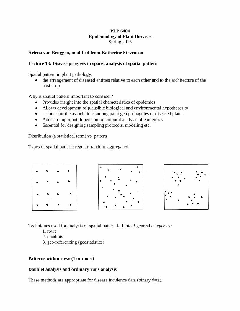
Types of spatial pattern: regular, random, aggregated

Techniques used for analysis of spatial pattern fall into 3 general categories:

1. rows

2. quadrats

3. geo-referencing (geostatistics)

Patterns within rows (1 or more)

Doublet analysis and ordinary runs analysis

These methods are appropriate for disease incidence data (binary data).

Example: + - - - + + - + - - + + + - -

+ = diseased plant - = healthy plant total # of plants in row = 15

Number of runs (U) = 8

If the pattern of diseased plants is random, then:

where, m = #infected plants in a row, N = #plants in the row

U will be less than E(U) if there is clustering. How much less depends on s(U):

Calculate a Z-statistic (standard normal distribution):

if Z is less than -1.64, then conclude clustering (P=0.05)

Note: must have N>20 for normal assumption to hold.

Quadrat-based analyses

5 basic approaches to spatial pattern analysis based on quadrat count data:

1. mapping

2. evaluating goodness-of-fit of particular distributions to frequency counts

3. calculating index of dispersion

4. calculating variances of blocked quadrats

5. spatial autocorrelation among quadrats

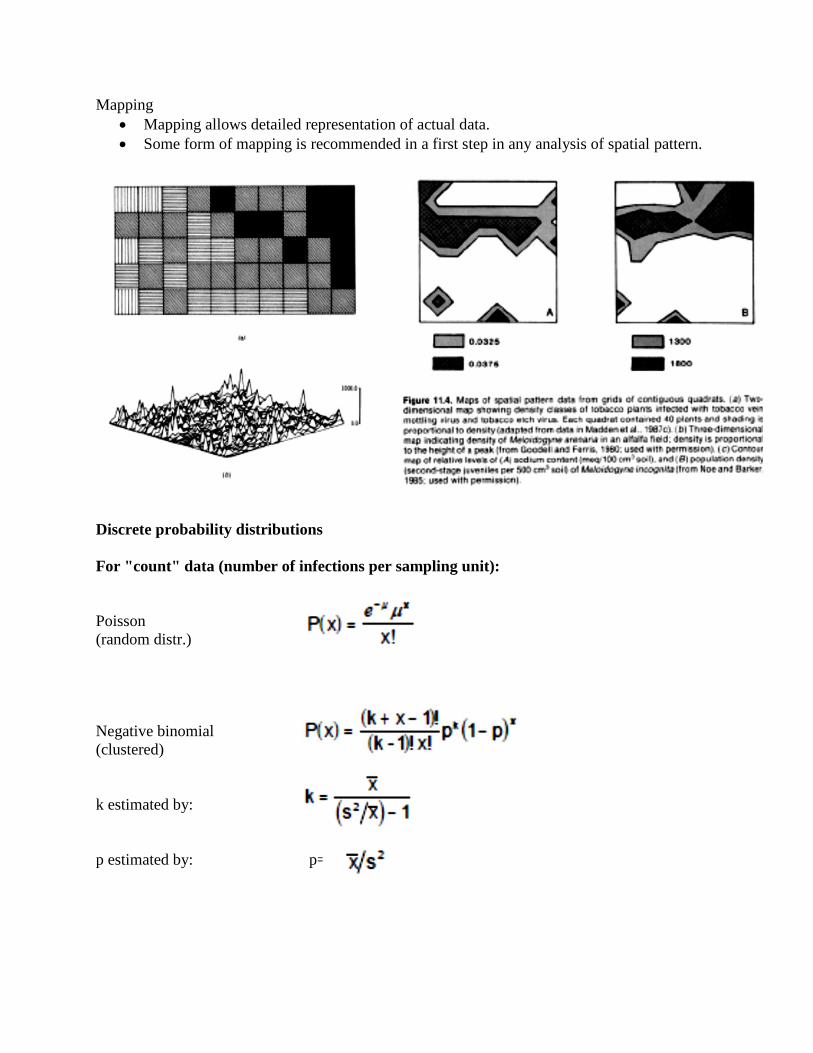
Mapping

Mapping allows detailed representation of actual data.

Some form of mapping is recommended in a first step in any analysis of spatial pattern.

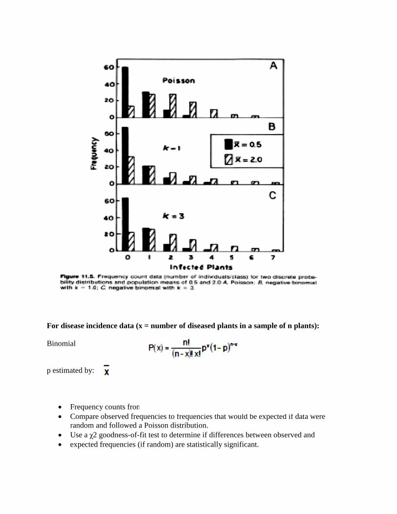
Discrete probability distributions

For "count" data (number of infections per sampling unit):

Poisson

(random distr.)

Negative binomial

(clustered)

k estimated by:

p estimated by: p=

For disease incidence data (x = number of diseased plants in a sample of n plants):

Binomial

p estimated by:

Frequency counts from quadrats are represented by a histogram.

Compare observed frequencies to frequencies that would be expected if data were

random and followed a Poisson distribution.

Use a χ2 goodness-of-fit test to determine if differences between observed and

expected frequencies (if random) are statistically significant.

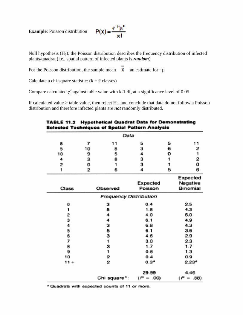
Example: Poisson distribution

Null hypothesis (H0): the Poisson distribution describes the frequency distribution of infected

plants/quadrat (i.e., spatial pattern of infected plants is random)

For the Poisson distribution, the sample mean, , is an estimate for : µ

Calculate a chi-square statistic: (k = # classes)

Compare calculated χ2 against table value with k-1 df, at a significance level of 0.05

If calculated value > table value, then reject H0, and conclude that data do not follow a Poisson

distribution and therefore infected plants are not randomly distributed.

Things to be aware of when using this approach:

χ2 test is not very powerful, especially with small sample sizes.

The fit of a particular distribution alone is not sufficient evidence to conclude how the

spatial pattern arose.

Index of dispersion (D)

- provides a measure of the degree of spatial aggregation in a population

For count data (variance-to-mean ratio):

where s2 is the sample variance and 0 is the sample mean

For disease incidence data:

D<1 Regular pattern

D=1 Random pattern

D>1 Aggregated pattern

To test for deviations from randomness, compare (N - 1) D to χ2 with N – 1 df, where N = total

number of sampling units (e.g. quadrats); If (N – 1) D is greater than the table value, then

conclude not random

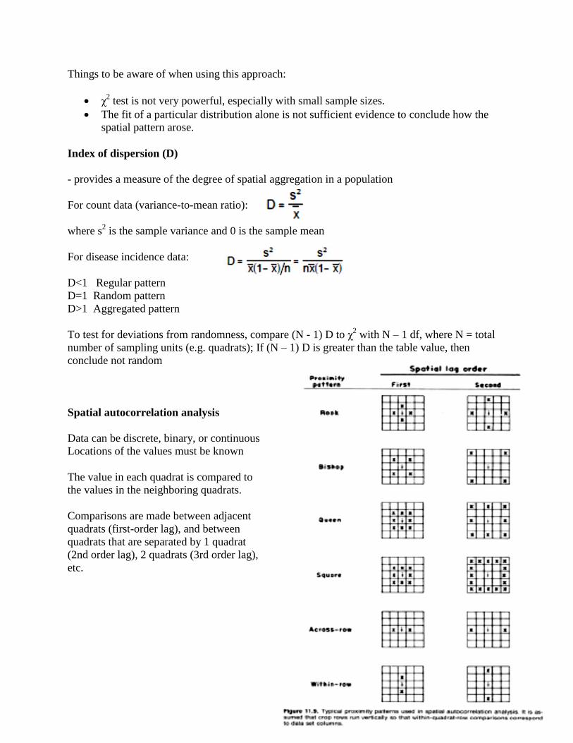
Spatial autocorrelation analysis

Data can be discrete, binary, or continuous

Locations of the values must be known

The value in each quadrat is compared to

the values in the neighboring quadrats.

Comparisons are made between adjacent

quadrats (first-order lag), and between

quadrats that are separated by 1 quadrat

(2nd order lag), 2 quadrats (3rd order lag),

etc.

Index of dispersion vs. spatial autocorrelation

Index of dispersion and frequency distribution techniques can be used only for discrete

data such as counts per quadrat.

Spatial autocorrelation can be used for discrete or continuous data

Spatial autocorrelation also takes into account location of individual plants or sampling

units.

GIS and Geostatistics

Uses of GIS and geostatistics in plant disease epidemiology:

to store and query spatially referenced point data

to generate maps of pathogens or diseases and risk of diseases

(See: Nelson, M. R., Orum, T. V., Jaime-Garcia, R., and Nadeem, A., 1999. Applications

of geographic information systems and geostatistics in plant disease epidemiology and

management. Plant Disease 83:308-319)

Geographic Information Systems (GIS)

a computer-based system capable of assembling, storing, manipulating, and displaying

data referenced by geographic coordinates.

has the ability to integrate layers of spatial information and to uncover possible

relationships that would not otherwise be obvious

Software programs: ArcView, MapInfo, SAS GIS

GIS is the most common way of spatial analysis these days, but you need to take one or more

separate courses to learn these techniques. We will not discuss GIS in this class.

Geostatistics

Statistical methods for analysis of spatially distributed variables and the prediction or estimation

of values at unsampled locations.

Geostatistical analysis can be broken down into 4 phases:

exploratory data analysis

estimation and modeling of spatial autocorrelation (semivariance estimation)

estimating values at unsampled locations ("kriging" a method of surface

interpolation)

evaluation of reliability of estimates

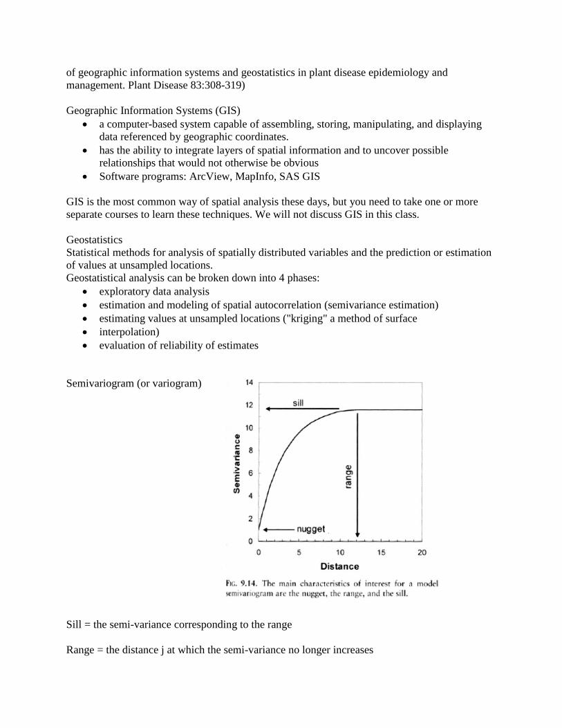
Semivariogram (or variogram)

Sill = the semi-variance corresponding to the range

Range = the distance j at which the semi-variance no longer increases

Nugget = the semi-variance at distance j=0 between sampling units

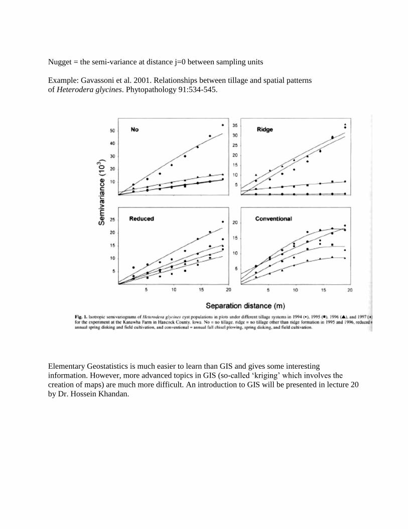
Example: Gavassoni et al. 2001. Relationships between tillage and spatial patterns

of Heterodera glycines. Phytopathology 91:534-545.

Elementary Geostatistics is much easier to learn than GIS and gives some interesting

information. However, more advanced topics in GIS (so-called ‘kriging’ which involves the

creation of maps) are much more difficult. An introduction to GIS will be presented in lecture 20

by Dr. Hossein Khandan.