Embed Size (px)
Citation preview
POLAR REED-SOLOMON CONCATENATEDCODES FOR OPTICAL COMMUNICATIONS
a thesis submitted to
the graduate school of engineering and science
of bilkent university
in partial fulfillment of the requirements for
the degree of
master of science
in
electrical and electronics engineering
By
Yigit Ertugrul
July 2020

Polar Reed-Solomon Concatenated Codes for Optical Communications
By Yigit Ertugrul
July 2020
We certify that we have read this thesis and that in our opinion it is fully adequate,
in scope and in quality, as a thesis for the degree of Master of Science.
Erdal Arıkan (Advisor)
Tolga Mete Duman
Ali Ozgur Yılmaz
Approved for the Graduate School of Engineering and Science:
Ezhan KarasanDirector of the Graduate School
ii
ABSTRACT
POLAR REED-SOLOMON CONCATENATED CODESFOR OPTICAL COMMUNICATIONS
Yigit Ertugrul
M.S. in Electrical and Electronics Engineering
Advisor: Erdal Arıkan
July 2020
A concatenated forward error correcting (FEC) code is developed by targeting
optical communications. Polar and product Reed-Solomon (RS) codes are used as
inner and outer codes, respectively. An interleaver block is designed to align mul-
tiple inner code blocks. Target key parameter indicators (KPIs) for the decoder
circuitry are set to 1 Tb/s throughput and 10 mm2 area occupation. These KPIs
narrowed the design space down to the simplest decoding algorithms in moderate
block-lengths. Soft information from the channel is collected by a polar decoder.
Minimum distance between codewords is increased by a product code with two
error correcting RS codes. Performance of the developed FEC code is evaluated
based on its communications performance, decoding complexity and area occu-
pation. Code configurations are designed with overheads of 15%, 20%, 24% and
28% supporting 1 Tb/s throughput. In one configuration, 11.3 dB net coding
gain is estimated at 10−15 bit error rate (BER). Area of the decoder circuitry is
estimated to be 14.27 mm2 in 28nm while supporting 1 Tb/s throughput.
Keywords: error-correcting codes, polar codes, Reed Solomon codes, optical com-
munications.
iii
OZET
OPTIK HABERLESME ICIN UC UCA EKLEMELIKUTUPSAL REED-SOLOMON KODLAR
Yigit Ertugrul
Elektrik ve Elektronik Muhendisligi, Yuksek Lisans
Tez Danısmanı: Erdal Arıkan
Temmuz 2020
Optik hatlarda haberlesmeyi hedefleyen uc uca eklenmis bir hata duzeltme kodu
gelistirildi. Kutupsal ve Reed-Solomon (RS) carpım kodlar ic ve dıs kodlar olarak
kullanıldı. Birden fazla ic kodu dizmek icin bir harmanlayıcı blogu tasarlandı.
Kod cozucu devresi icin, saniye basına 1 terabit veri hızı ve 10 milimetrekare alan
performans belirleyici hedefler olarak belirlendi. Bu performans belirleyici hede-
fler, tasarım uzayını orta blok uzunluklarında en basit kod cozme algoritmalarına
kadar daralttı. Kanaldaki yumusak bilgi bir kutupsal kod cozucu tarafından
toplandı. Kod kelimeleri arasındaki en az mesafe iki hata duzelten RS kod kul-
lanan carpım kodları ile artırıldı. Gelistirilen hata duzeltme kodunun perfor-
mansı; iletisim performansı, kod cozme karmasıklıgı ve kapladıgı alan baz alınarak
degerlendirildi. Saniye basına 1 terabit veri hızında %15, %20, %24 ve %28 fa-
zlalık oranlarında kod tasarımları yapıldı. Bir tasarımda, 10−15 bit hata oranında
11.3 dB net kodlama kazancı kestirimi yapıldı. Saniye basına 1 terabit veri hızını
saglayan kod cozucu devresinin alanı 28nm teknolojisinde 14.27 milimetrekare
olarak kestirildi.
Anahtar sozcukler : hata duzelten kodlar, kutupsal kodlar, Reed-Solomon kodlar,
optik haberlesme.
iv

Acknowledgement
I would like to thank my supervisor, Prof. Erdal Arıkan for his persistent support,
encouragement and patience during my thesis. I would like to thank my thesis
jury members, Prof. Tolga Mete Duman and Prof. Ali Ozgur Yılmaz for their
comments that elevated the quality of this thesis.
I would like to thank Bilkent University for giving me the opportunity to study
here. I would like to thank EPIC project which is funded by the European
Union’s Horizon 2020 research and innovation programme under grant agreement
No 760150.
In particular, I would like to thank Ertugrul Kolagasıoglu for his support and
teachings that motivated this thesis.
I am indebted to my colleagues in Polaran. I would like to thank Altug Sural
and Evren Goksu Sezer for the invaluable technical discussions. I would like to
thank my family for their support throughout my educational career.
v
Contents
1 Introduction 1
1.1 Fiber-Optic Use Case . . . . . . . . . . . . . . . . . . . . . . . . . 5
1.2 Literature Survey . . . . . . . . . . . . . . . . . . . . . . . . . . . 6
1.2.1 First and Second Generation Codes . . . . . . . . . . . . . 7
1.2.2 Third Generation Codes . . . . . . . . . . . . . . . . . . . 9
1.3 Aim of the Thesis . . . . . . . . . . . . . . . . . . . . . . . . . . . 14
1.4 Summary of Main Results . . . . . . . . . . . . . . . . . . . . . . 14
1.5 Outline of Thesis . . . . . . . . . . . . . . . . . . . . . . . . . . . 16
2 Review of Codes 17
2.1 Polar Codes . . . . . . . . . . . . . . . . . . . . . . . . . . . . . . 17
2.1.1 Notations . . . . . . . . . . . . . . . . . . . . . . . . . . . 18
2.1.2 Preliminaries . . . . . . . . . . . . . . . . . . . . . . . . . 18
2.1.3 Channel Polarization . . . . . . . . . . . . . . . . . . . . . 19
vi
CONTENTS vii
2.1.4 Polar Encoding . . . . . . . . . . . . . . . . . . . . . . . . 20
2.1.5 Code Construction Methods . . . . . . . . . . . . . . . . . 22
2.1.6 Systematic Polar Coding . . . . . . . . . . . . . . . . . . . 22
2.1.7 Decoding Algorithms . . . . . . . . . . . . . . . . . . . . . 25
2.2 Reed-Solomon Codes . . . . . . . . . . . . . . . . . . . . . . . . . 32
2.2.1 Analytical Error Performance and Emulation Methods . . 32
2.3 Product Codes . . . . . . . . . . . . . . . . . . . . . . . . . . . . 35
2.4 Concatenated Codes . . . . . . . . . . . . . . . . . . . . . . . . . 36
2.5 Summary of the Chapter . . . . . . . . . . . . . . . . . . . . . . . 36
3 RS2-Polar Concatenation Scheme 37
3.1 Outer Encoder . . . . . . . . . . . . . . . . . . . . . . . . . . . . 40
3.2 Interleaver & Segmentation . . . . . . . . . . . . . . . . . . . . . 42
3.3 Inner Encoder & Decoder Pairs . . . . . . . . . . . . . . . . . . . 44
3.3.1 Polar(512,416) SC List4 . . . . . . . . . . . . . . . . . . . 46
3.3.2 Polar(2048,1664) SC . . . . . . . . . . . . . . . . . . . . . 46
3.3.3 Polar(1024,882) SC . . . . . . . . . . . . . . . . . . . . . . 46
3.3.4 Polar(2048,1704) SC . . . . . . . . . . . . . . . . . . . . . 47
3.3.5 Polar(2048,1776) SC . . . . . . . . . . . . . . . . . . . . . 47
3.3.6 Polar(2048,1832) SC . . . . . . . . . . . . . . . . . . . . . 47
CONTENTS viii
3.4 Outer Decoder . . . . . . . . . . . . . . . . . . . . . . . . . . . . 48
3.5 Simulation Results . . . . . . . . . . . . . . . . . . . . . . . . . . 49
3.6 Complexity Analysis . . . . . . . . . . . . . . . . . . . . . . . . . 56
3.6.1 Hardware Complexity . . . . . . . . . . . . . . . . . . . . 57
3.7 Comparison with Other Codes . . . . . . . . . . . . . . . . . . . . 59
3.8 Summary of the Chapter . . . . . . . . . . . . . . . . . . . . . . . 60
4 Conclusion 61
A Interleaver 71
List of Figures
1.1 Block diagram of a generic communication system. . . . . . . . . 1
1.2 Capacity versus Es/No (dB). . . . . . . . . . . . . . . . . . . . . . 3
1.3 Achievable FER performance of finite block-length codes. . . . . . 4
1.4 FEC hard and soft decision net coding gains. . . . . . . . . . . . . 9
2.1 The channel W2 is constructed from two independent copies of W . 19
2.2 Length 8 polar encoder. . . . . . . . . . . . . . . . . . . . . . . . 21
2.3 BER performance of rate 0.5 polar codes under SC decoding on
AWGN channel and BPSK modulation. . . . . . . . . . . . . . . . 23
2.4 FER performance of rate 0.5 polar codes under SC decoding on
AWGN channel and BPSK modulation. . . . . . . . . . . . . . . . 24
2.5 BER performance of rate 0.5 polar codes under SC decoding on
AWGN channel and BPSK modulation. . . . . . . . . . . . . . . . 27
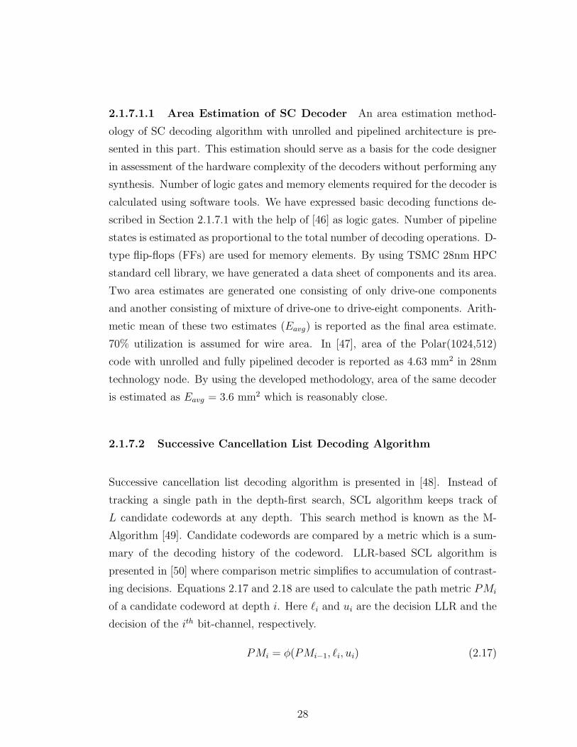
2.6 FER performance of rate 0.5 polar codes under SC decoding on
AWGN channel and BPSK modulation. . . . . . . . . . . . . . . . 27
ix
LIST OF FIGURES x
2.7 BER performance of rate 0.5 polar codes under SCL decoding on
AWGN channel and BPSK modulation. . . . . . . . . . . . . . . . 30
2.8 FER performance of rate 0.5 polar codes under SCL decoding on
AWGN channel and BPSK modulation. . . . . . . . . . . . . . . . 31
2.9 BER performance comparison between simulations and analytical
estimations. . . . . . . . . . . . . . . . . . . . . . . . . . . . . . . 33
2.10 FER performance comparison between simulations and analytical
estimations. . . . . . . . . . . . . . . . . . . . . . . . . . . . . . . 34
2.11 Product code structure with component codes C1(N1, K1) and
C2(N2, K2). . . . . . . . . . . . . . . . . . . . . . . . . . . . . . . 35
3.1 Transmitter and receiver chain. . . . . . . . . . . . . . . . . . . . 38
3.2 Product RS code structure. . . . . . . . . . . . . . . . . . . . . . 41
3.3 Interleaver & segmentation alignment for n = 15 and q = 3. . . . 43
3.4 BER performance comparison of inner polar codes and decoder
pairs on AWGN channel and BPSK modulation. . . . . . . . . . 45
3.5 FER performance comparison of inner polar codes and decoder
pairs on AWGN channel and BPSK modulation. . . . . . . . . . 45
3.6 BER performance of rate 0.96 product RS code with RS8(208,204)
component code. 6 decoding iterations on AWGN channel and
BPSK modulation. . . . . . . . . . . . . . . . . . . . . . . . . . . 48
3.7 BER performance of rate 0.78 (28% OH) RS2-Polar code under
SC List 4 decoding and 6 iterations on AWGN channel and BPSK
modulation. . . . . . . . . . . . . . . . . . . . . . . . . . . . . . 50
LIST OF FIGURES xi
3.8 BER performance of rate 0.78 (28% OH) RS2-Polar code under SC
decoding and 6 iterations on AWGN channel and BPSK modulation. 51
3.9 BER performance of rate 0.80 (24% OH) RS2-Polar code under SC
decoding and 6 iterations on AWGN channel and BPSK modulation. 52
3.10 BER performance of rate 0.80 (24% OH) RS2-Polar code on
AWGN channel and BPSK modulation. . . . . . . . . . . . . . . . 53
3.11 BER performance of rate 0.83 (20% OH) RS2-Polar code on
AWGN channel and BPSK modulation. . . . . . . . . . . . . . . . 54
3.12 BER performance of rate 0.87 (15% OH) RS2-Polar code on
AWGN channel and BPSK modulation. . . . . . . . . . . . . . . . 55
3.13 Hierarchical floor-planning of RS2-Polar decoder. . . . . . . . . . 58
List of Tables
1.1 Comparison with first and second generation coding schemes. . . . 8
1.2 Comparison with third generation coding schemes. . . . . . . . . . 10
1.3 Communications performance and parameters of developed FEC
codes. . . . . . . . . . . . . . . . . . . . . . . . . . . . . . . . . . 15
3.1 Outer code parameters. . . . . . . . . . . . . . . . . . . . . . . . . 41
3.2 Inner code parameters of various code configurations. . . . . . . . 44
3.3 Performance of developed RS2-Polar codes. . . . . . . . . . . . . . 49
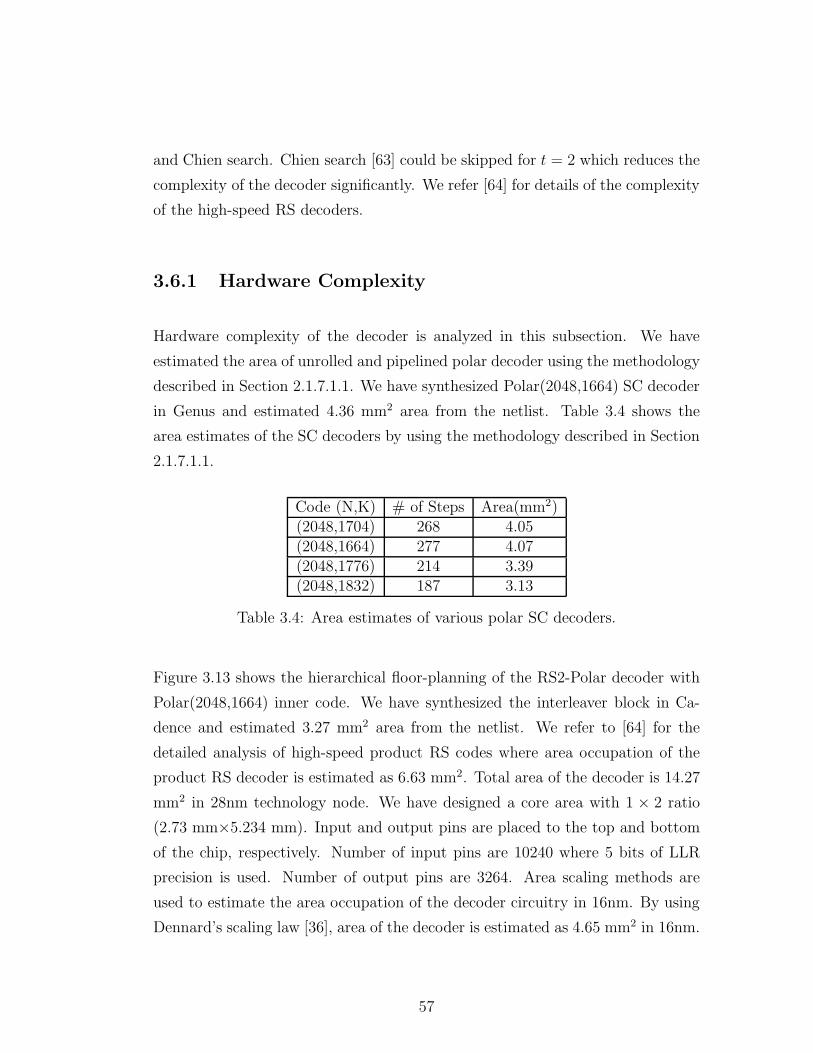
3.4 Area estimates of various polar SC decoders. . . . . . . . . . . . . 57
4.1 Performance results of the developed codes. . . . . . . . . . . . . 63
xii
Chapter 1
Introduction
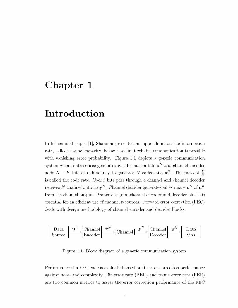
In his seminal paper [1], Shannon presented an upper limit on the information
rate, called channel capacity, below that limit reliable communication is possible
with vanishing error probability. Figure 1.1 depicts a generic communication
system where data source generates K information bits uK and channel encoder
adds N − K bits of redundancy to generate N coded bits xN . The ratio of KN
is called the code rate. Coded bits pass through a channel and channel decoder
receives N channel outputs yN . Channel decoder generates an estimate uK of uK
from the channel output. Proper design of channel encoder and decoder blocks is
essential for an efficient use of channel resources. Forward error correction (FEC)
deals with design methodology of channel encoder and decoder blocks.
DataSource
ChannelEncoder
ChannelChannelDecoder
DataSink
uK xN yN uK
Figure 1.1: Block diagram of a generic communication system.
Performance of a FEC code is evaluated based on its error correction performance
against noise and complexity. Bit error rate (BER) and frame error rate (FER)
are two common metrics to assess the error correction performance of the FEC
1
code. BER is the ratio of the number of bit errors to the number of information
bits. FER is the ratio of corrupted frames to the transmitted frames where a
frame is corrupted if at least one-bit error occurs. Complexity of a FEC code
could be evaluated by asymptotic runtime complexity and hardware complexity
in terms of area occupation. Landau notation is used to denote the asymptotic
runtime complexity of a FEC code. Area occupation is the measure of required
space for the decoding circuitry in mm2 units.
In this thesis, we focus on additive white Gaussian noise (AWGN) channel
and binary phase shift keying (BPSK) modulation. Define the AWGN channel
as y = x + z where y is the channel output, x is the channel input and z is the
additive Gaussian noise term with zero mean and No/2 variance. Signal-to-noise
ratio (SNR) is denoted by Es/No = 1σ2 . In BPSK modulation, bit energy Eb
(joule/bit) and signal energy Es (joule/2D) is related as 2REb = Es where R
(bit/D) is the code rate.
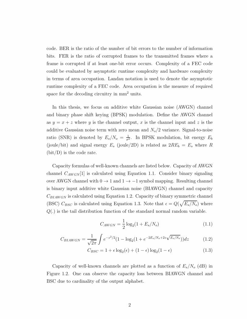
Capacity formulas of well-known channels are listed below. Capacity of AWGN
channel CAWGN [1] is calculated using Equation 1.1. Consider binary signaling
over AWGN channel with 0 → 1 and 1 → −1 symbol mapping. Resulting channel
is binary input additive white Gaussian noise (BIAWGN) channel and capacity
CBIAWGN is calculated using Equation 1.2. Capacity of binary symmetric channel
(BSC) CBSC is calculated using Equation 1.3. Note that ǫ = Q(√
Es/No) where
Q(.) is the tail distribution function of the standard normal random variable.
CAWGN =1
2log2(1 + Es/No) (1.1)
CBIAWGN =1√2π
∫
e−z2/2(1− log2(1 + e−2Es/No+2z√
Es/No))dz (1.2)
CBSC = 1 + ǫ log2(ǫ) + (1− ǫ) log2(1− ǫ) (1.3)
Capacity of well-known channels are plotted as a function of Es/No (dB) in
Figure 1.2. One can observe the capacity loss between BIAWGN channel and
BSC due to cardinality of the output alphabet.
2
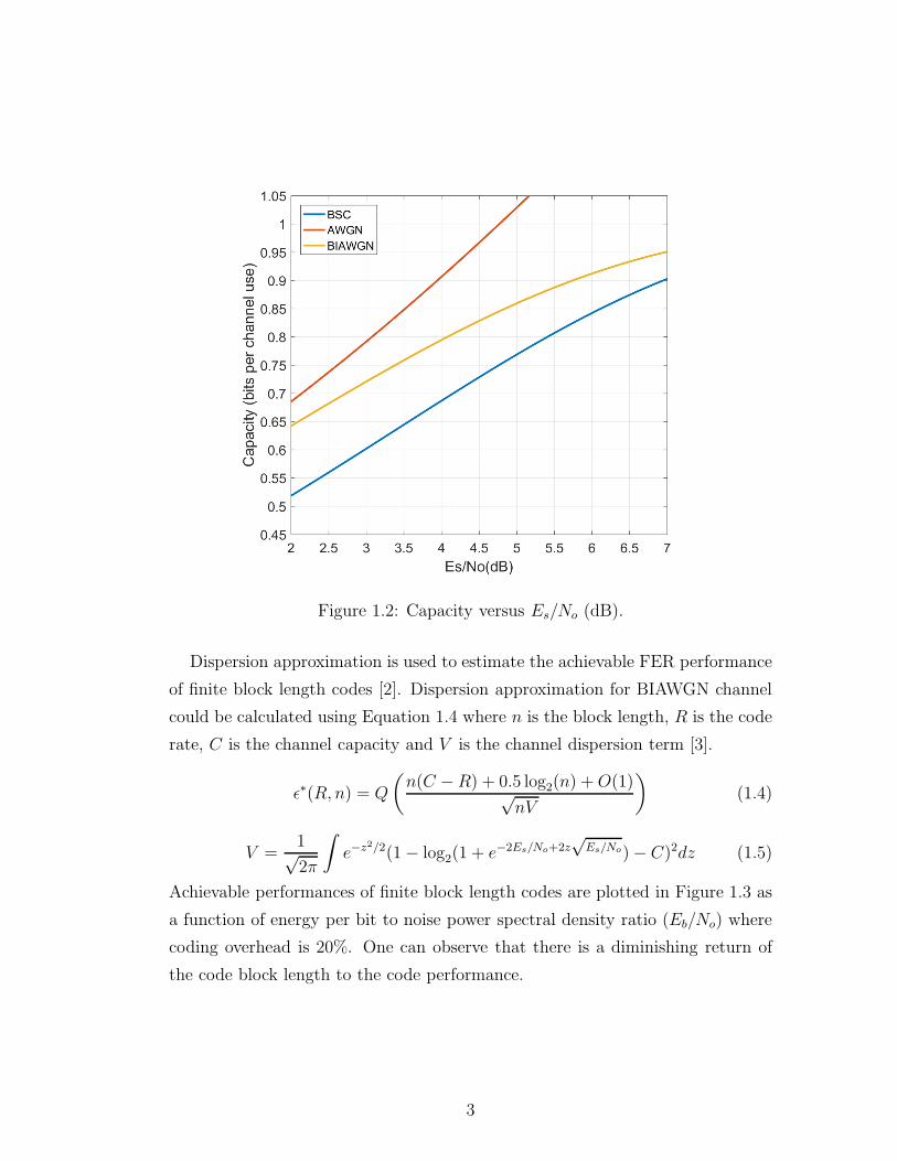
Figure 1.2: Capacity versus Es/No (dB).
Dispersion approximation is used to estimate the achievable FER performance
of finite block length codes [2]. Dispersion approximation for BIAWGN channel
could be calculated using Equation 1.4 where n is the block length, R is the code
rate, C is the channel capacity and V is the channel dispersion term [3].
ǫ∗(R, n) = Q
(
n(C −R) + 0.5 log2(n) +O(1)√nV
)
(1.4)
V =1√2π
∫
e−z2/2(1− log2(1 + e−2Es/No+2z√
Es/No)− C)2dz (1.5)
Achievable performances of finite block length codes are plotted in Figure 1.3 as
a function of energy per bit to noise power spectral density ratio (Eb/No) where
coding overhead is 20%. One can observe that there is a diminishing return of
the code block length to the code performance.
3
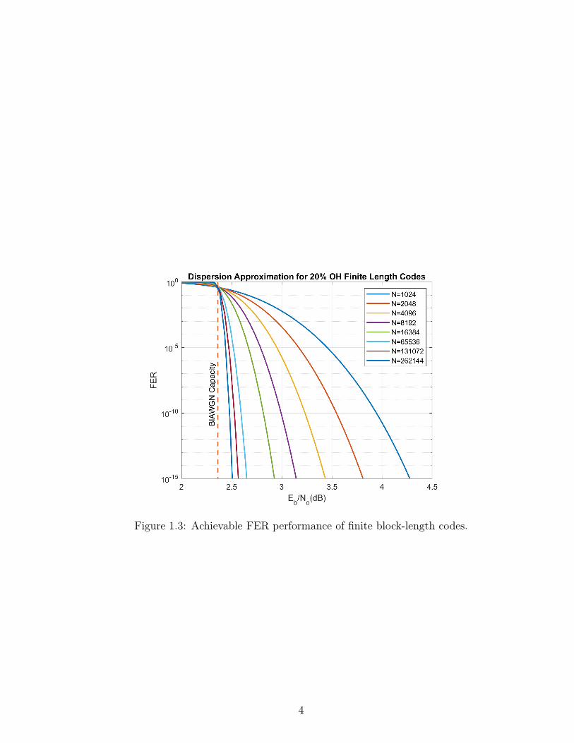
Figure 1.3: Achievable FER performance of finite block-length codes.
4
1.1 Fiber-Optic Use Case
Network operators are seeking ways of increasing the network capacity to address
the traffic growth problem [4]. Communication systems with higher data rates
have become favorable in this setting. A desirable solution would operate with
the existing physical structures from cabling to bandwidth allocation. To that
end, FEC is a viable component that compensates the non-ideal channel effects
while progressing to higher data rates.
Optical transport network (OTN) is an interface between digital domain and
optical media network [5]. This interface ensures multiplexing, routing, supervi-
sion and performance survivability for digital clients. Digital structure of OTN
contains multiple optical transport units (OTUs). Ethernet protocol is developed
by the Institution of Electrical and Electronics Engineers (IEEE) [6] which can
operate on both coaxial cable and optical medium. Data rates from 50 Gb/s to
400 Gb/s are supported over a single-mode fiber in [7]. A comparison of OTN and
Ethernet from network level could be found in [8]. FEC is a significant compo-
nent of OTN since transmission ranges are over 10 km where channel impairments
occur. Moreover, retransmission may not be favorable due to large propagation
delays. On the other hand, Ethernet does not use FEC to protect the data in the
short-range transmissions.
Roadmap of optical communications [4] identifies that the energy efficiency will
be one of the biggest challenges of FEC algorithms while supporting higher data
rates. In [9], authors discuss the implementation challenges for energy efficient
FEC. Impact of FEC on the energy consumption of optical transmitters is ana-
lyzed in [10] for short-range optical links. Authors show that FEC can reduce the
energy consumption of the transmitter by reducing the transmit power. There
is no doubt that energy efficiency will be a distinctive metric among candidate
FEC codes.
International Telecommunication Union (ITU) defined a standard for opti-
cal fiber submarine cable systems targeting 10−15 post-FEC BER [11]. We will
5
benefit from certain metrics in comparison of candidate FEC codes for optical
communications. Coding overhead (OH) denotes the amount of redundancy per
information bit and is a function of code rate OH = ( 1R− 1) × 100 in percent.
Pre-FEC uncoded BER (BERpre) denotes the raw BER at the decoder output
and is calculated as in Equation 1.6. Post-FEC BER (BERpost) denotes the BER
at the decoder output, the target is 10−15. Gap to Shannon limit could be calcu-
lated as in Equation 1.7 where Q−1(.) is the inverse of tail distribution function
of standard normal random variable. Net Coding Gain (NCG) is the measure of
reduction in the transmit power compared to uncoded transmission and could be
calculated as in Equation 1.8.
BERpre = Q(
√
2REb/No
)
(1.6)
GapBIAWGN = C−1BIAWGN(R)−
(
Q−1 (BERpost))2
/(2R) (1.7)
NCG =(
Q−1 (BERpost))2
/(2R)− Eb/No (1.8)
A FEC code could have different hardware realizations exploiting different
architectural templates. In [12], authors identified the practical limits of the
well-known channel codes from an implementation point of view. 10 mm2 area
occupation under 1 Tb/s throughput is identified by Enabling Practical Wire-
less Tb/s Communications with Next Generation Channel Coding (EPIC) [13]
project. These targets are identified only for the decoding circuitry in advanced
technology nodes (7/16/28nm). Keeping the data rate, performance and area
metrics in mind, a desirable FEC code should exhibit the best of three metrics
compared to others.
1.2 Literature Survey
A comprehensive survey of the FEC codes that are suitable for fiber-optic use
case are presented in this section. In this field of study, FEC codes are divided
into three generations namely first, second and third. First and second-generation
6
codes are explained in Section 1.2.1. Third generation codes propose more sophis-
ticated FEC code schemes. These codes are presented in Section 1.2.2. Commu-
nications performance of the codes will be evaluated based on coding overhead,
pre-FEC uncoded BER, post-FEC coded BER and gap to Shannon limit at BER
10−15.
1.2.1 First and Second Generation Codes
First and second-generation codes are presented in this subsection. In [11], ITU
defines a Reed-Solomon (RS) code for multigigabit-per-second optical fiber sub-
marine cable systems. Systematic RS(255,239) code with 7% overhead is used to
protect the data to be transmitted. This code is capable of correcting 2t+e ≤ 16
errors and erasures. Depending on the interleaver depth n, a FEC frame is
2040× n bits long.
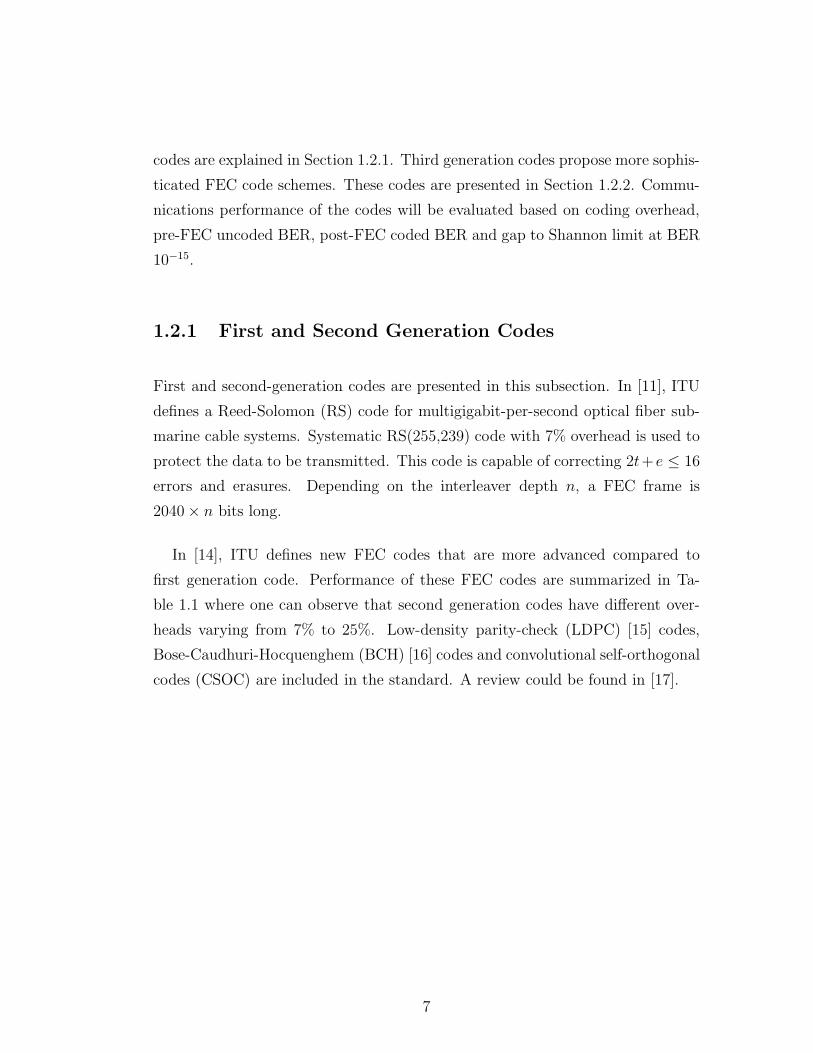
In [14], ITU defines new FEC codes that are more advanced compared to
first generation code. Performance of these FEC codes are summarized in Ta-
ble 1.1 where one can observe that second generation codes have different over-
heads varying from 7% to 25%. Low-density parity-check (LDPC) [15] codes,
Bose-Caudhuri-Hocquenghem (BCH) [16] codes and convolutional self-orthogonal
codes (CSOC) are included in the standard. A review could be found in [17].
7
Code OverheadBlockLength(bits)
BIAWGNShannonLimit at R
Pre-FECBER
UncodedEb/No
Post-FECBERCodedEb/No
Gap toShannonLimit dB
RS(255,239) 7% 2040 3.8238.404e-58.499 dB
1e-158.781 dB
4.97
CSOC×RS 24.48% 32640 2.075.226e-35.156 dB
1e-156.107 dB
4.577
BCH×BCH 6.69% 32640 3.8833.217e-35.696 dB
1e-155.997 dB
2.09
BCH×RS 7% 130560 3.8232.332e-36.023 dB
1e-156.317 dB
2.494
pr.Hamming×RS 6.69% 261120 3.8834.594e-35.305 dB
1e-155.587 dB
1.704
LDPC 6.69% 32640 3.8831.533e-36.418 dB
1e-156.7 dB
2.81
BCH×BCH 7% 32640 3.8231.245e-36.603 dB
1e-156.897 dB
3.074
BCH×BCH 11% 33536 3.2124.443e-35.344 dB
1e-155.797 dB
2.585
BCH×BCH 25% 38016 2.041.286e-23.958 dB
1e-154.927 dB
2.887
RS 7% 32640 3.8231.112e-36.699 dB
1e-156.98 dB
3.16
Table 1.1: Comparison with first and second generation coding schemes.
8
1.2.2 Third Generation Codes
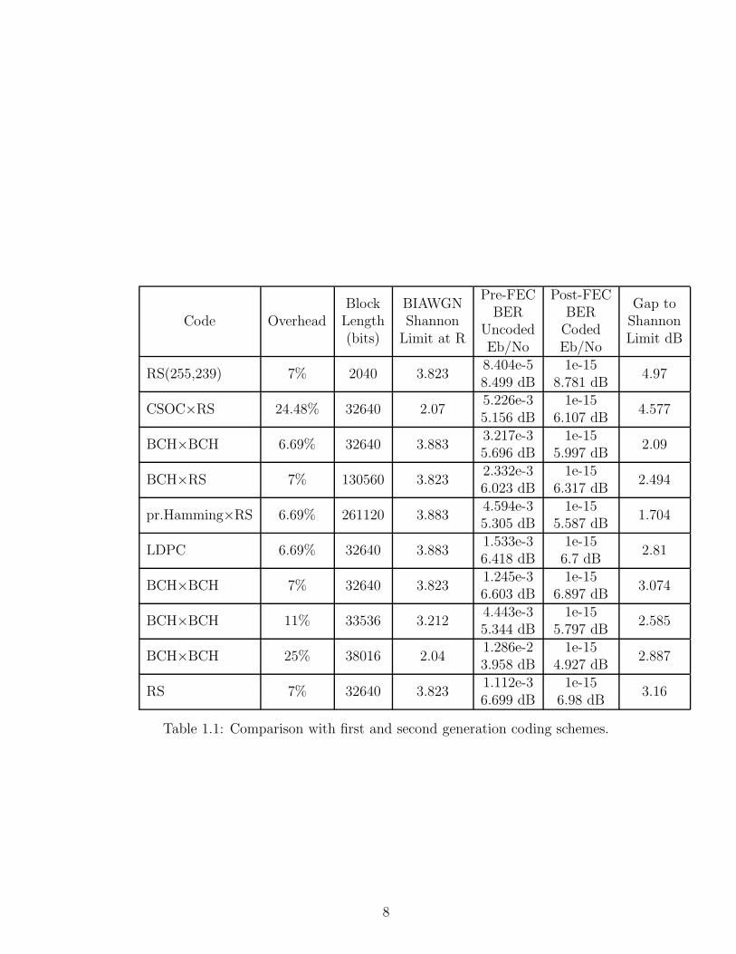
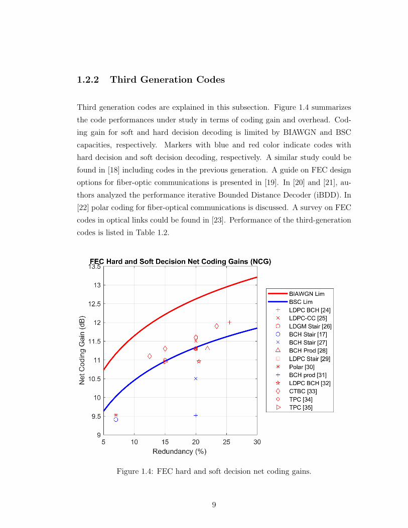
Third generation codes are explained in this subsection. Figure 1.4 summarizes
the code performances under study in terms of coding gain and overhead. Cod-
ing gain for soft and hard decision decoding is limited by BIAWGN and BSC
capacities, respectively. Markers with blue and red color indicate codes with
hard decision and soft decision decoding, respectively. A similar study could be
found in [18] including codes in the previous generation. A guide on FEC design
options for fiber-optic communications is presented in [19]. In [20] and [21], au-
thors analyzed the performance iterative Bounded Distance Decoder (iBDD). In
[22] polar coding for fiber-optical communications is discussed. A survey on FEC
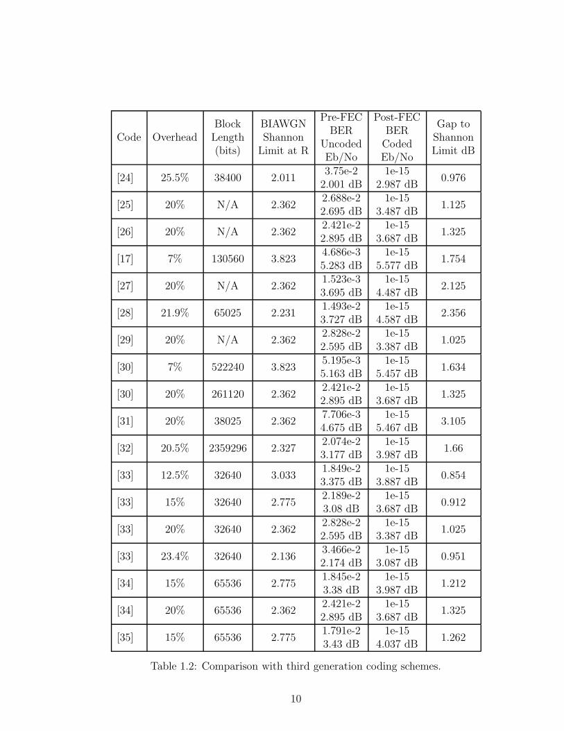
codes in optical links could be found in [23]. Performance of the third-generation
codes is listed in Table 1.2.
Figure 1.4: FEC hard and soft decision net coding gains.
9
Code OverheadBlockLength(bits)
BIAWGNShannonLimit at R
Pre-FECBER
UncodedEb/No
Post-FECBERCodedEb/No
Gap toShannonLimit dB
[24] 25.5% 38400 2.0113.75e-22.001 dB
1e-152.987 dB
0.976
[25] 20% N/A 2.3622.688e-22.695 dB
1e-153.487 dB
1.125
[26] 20% N/A 2.3622.421e-22.895 dB
1e-153.687 dB
1.325
[17] 7% 130560 3.8234.686e-35.283 dB
1e-155.577 dB
1.754
[27] 20% N/A 2.3621.523e-33.695 dB
1e-154.487 dB
2.125
[28] 21.9% 65025 2.2311.493e-23.727 dB
1e-154.587 dB
2.356
[29] 20% N/A 2.3622.828e-22.595 dB
1e-153.387 dB
1.025
[30] 7% 522240 3.8235.195e-35.163 dB
1e-155.457 dB
1.634
[30] 20% 261120 2.3622.421e-22.895 dB
1e-153.687 dB
1.325
[31] 20% 38025 2.3627.706e-34.675 dB
1e-155.467 dB
3.105
[32] 20.5% 2359296 2.3272.074e-23.177 dB
1e-153.987 dB
1.66
[33] 12.5% 32640 3.0331.849e-23.375 dB
1e-153.887 dB
0.854
[33] 15% 32640 2.7752.189e-23.08 dB
1e-153.687 dB
0.912
[33] 20% 32640 2.3622.828e-22.595 dB
1e-153.387 dB
1.025
[33] 23.4% 32640 2.1363.466e-22.174 dB
1e-153.087 dB
0.951
[34] 15% 65536 2.7751.845e-23.38 dB
1e-153.987 dB
1.212
[34] 20% 65536 2.3622.421e-22.895 dB
1e-153.687 dB
1.325
[35] 15% 65536 2.7751.791e-23.43 dB
1e-154.037 dB
1.262
Table 1.2: Comparison with third generation coding schemes.
10
Spatially coupled LDPC codes are concatenated with BCH codes in [24]
where code block length equals 38400 bits. LDPC(38400,30832) (24.5% over-
head) code is concatenated with BCH(30832,30592) (0.78% overhead) code.
BCH(30832,30592) code can correct 16-bit errors. Number of iterations is set
to 32 for LDPC decoder. Instead of min-sum algorithm, δ-min algorithm is used.
Simulation results are reported up to 10−11 BER.
LDPC convolutional code (LDPC-CC) is proposed in [25]. LDPC-
CC(10032,4,24) code has constraint length Lc equals 10032. Number of ones
at each column and row in the parity-check matrix is denoted by J and K, re-
spectively. Here J = 4 and K = 24. Layered decoding algorithm is used with 12
iterations.
Low-density generator matrix (LDGM) codes are concatenated with staircase
codes in [26]. Belief propagation algorithm with min-sum approximation is used
at the decoder. Complexity of the decoder is estimated by a score function. Code
performance is estimated by analytical methods.
BCH codes are concatenated with staircase codes in [17] where code block
length equals 130560 bits. BCH staircase codes are used with a syndrome-based
decoder. Component codes are BCH(1023,993,3). Performance of the decoder is
verified by field programmable gate array (FPGA) simulations.
BCH codes are concatenated with staircase codes in [27] where component code
is BCH(432,396,4). Number of iterations is set to 6. Coding gain is calculated
analytically. Decoder throughput achieves 1 Tb/s with around 2 pJ/b energy
efficiency at 28nm.
BCH codes are concatenated with product codes in [28] where code block
length equals 65025 bits. Product code is used with BCH(255,231,3) component
code. Iterative bounded-distance decoding with scaled reliability (iBDD-SR) de-
coder is used with 5 iterations. BER performance is estimated using extrapolation
methods. Decoder throughput achieves 1 Tb/s with 0.63 pJ/b energy efficiency
at 28nm.
11
LDPC codes are concatenated with staircase codes in [29]. Length 30000 and
6000 LDPC codes are used. Sum-product algorithm with floating-point message-
passing is used in simulations. Complexity of the decoder is estimated by a score
function. Code performance is estimated by analytical methods.
Polar codes are used in [30]. For 20% overhead, block length equals 522240
bits. Polar(522240,435200) code is decoded under successive cancellation (SC)
decoding algorithm. For 7% overhead, block length equals 261120 bits. Po-
lar(261120,244736) code is decoded under SC decoding algorithm. Communica-
tions performance is estimated with density evolution based Gaussian approxi-
mation (DE-GA).
BCH codes are concatenated with product codes in [31] where code block
length equals 38025 bits. Product BCH code is used with BCH(195,178) com-
ponent code. Extended BCH (eBCH) decoder is used for decoding. Decoder
achieves 100 Gb/s throughput at 65nm. Decoder throughput is 162 b/cycle at
worst case with post-processing iterations. Code performance is evaluated with
FPGA simulations up to 10−13 BER.
LDPC codes are concatenated with product BCH codes in [32] where code
block length equals 2359296 bits. Unequal error protection (UEP) BCH product
code is used as outer code and LDPC code is used as inner code. Component
codes are BCH(1632,1588) in one axis and BCH(1280,1236), BCH(1280,1255) in
the other axis. Inner code is LDPC(4608,4080) with 16 decoding iterations. BCH
product code is used with 8 decoding iterations. Extrapolation method is used
to estimate the code performance. Simulations are done up to 10−8 BER.
Constrained turbo block convolutional codes (CTBC) are used in [33] where
block length is 122368 message bits plus coding overhead bits. There are four code
designs with 12.5%, 15%, 20% and 23.4% OH. A BCH outer code, a constrained
interleaver and a recursive convolutional code is used as inner code. Bahl Cocke
Jelinek Raviv (BCJR) and Pyndiah algorithms are used to decode inner and outer
codes, respectively. Code performance is estimated analytically.
12
Turbo product codes (TPC) are used in [34] where block length is configurable
with OTU4 frames. There are two code designs with 15% and 20% overheads.
Performance of the codes is verified in software and hardware. In [35], a similar
turbo product code is developed where code block-length equals 65536 bits and
component code is an extended BCH(256,239) code.
13
1.3 Aim of the Thesis
Aim of this thesis is to develop a FEC code that could satisfy EPIC project targets
in advanced technology nodes. EPIC project aims to show Tb/s communications
is possible with well-known FEC codes. These targets are 10 mm2 area occupa-
tion and 1 Tb/s throughput. 1024 block-length polar codes under SC decoding
satisfied EPIC project targets. However, EPIC polar code has mediocre commu-
nications performance compared to codes in the literature. By using EPIC polar
code, our aim is to design a concatenated code that satisfies 1 Tb/s throughput
and has above 10.5 dB net coding gain at 10−15 BER. With the help of RS codes,
communications performance of the EPIC polar code is increased. In order to
concatenate these codes, RS codes must keep up the pace with EPIC polar codes
in terms of throughput. To that end, two-error correcting RS codes are used to
satisfy the throughput requirement. In this thesis, we will study the best way to
concatenate two FEC codes such that 1 Tb/s throughput is satisfied.
1.4 Summary of Main Results
A concatenated FEC code and architecture is developed that achieve 1 Tb/s
throughput, 11.3 dB coding gain under 10 mm2 in 16nm technology. Polar and
product-RS codes are used as inner and outer codes, respectively. Due to imple-
mentation constraints, a combination of low-complexity polar codes and simple
RS codes is used as component codes for iterative decoding. An interleaver be-
tween inner and outer code is employed such that polar frames are distributed
into product code in a specific way.
In one configuration, developed FEC code can achieve 11.5 dB net coding gain
at 10−15 BER with 28% overhead. Table 1.3 summarizes the code parameters
and communications performance of the developed codes. One of the developed
codes and corresponding architectures are synthesized using Cadence Genus with
Taiwan Semiconductor Manufacturing Company (TSMC) 28nm high performance
14
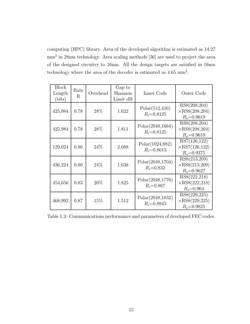
computing (HPC) library. Area of the developed algorithm is estimated as 14.27
mm2 in 28nm technology. Area scaling methods [36] are used to project the area
of the designed circuitry to 16nm. All the design targets are satisfied in 16nm
technology where the area of the decoder is estimated as 4.65 mm2.
BlockLength(bits)
RateR
OverheadGap toShannonLimit dB
Inner Code Outer Code
425,984 0.78 28% 1.622Polar(512,416)Ri=0.8125
RS8(208,204)×RS8(208,204)Ro=0.9619
425,984 0.78 28% 1.811Polar(2048,1664)
Ri=0.8125
RS8(208,204)×RS8(208,204)Ro=0.9619
129,024 0.80 24% 2.088Polar(1024,882)
Ri=0.8613
RS7(126,122)×RS7(126,122)Ro=0.9375
436,224 0.80 24% 1.638Polar(2048,1704)
Ri=0.832
RS8(213,209)×RS8(213,209)Ro=0.9627
454,656 0.83 20% 1.825Polar(2048,1776)
Ri=0.867
RS8(222,218)×RS8(222,218)
Ro=0.964
468,992 0.87 15% 1.512Polar(2048,1832)
Ri=0.8945
RS8(229,225)×RS8(229,225)Ro=0.9825
Table 1.3: Communications performance and parameters of developed FEC codes.
15
1.5 Outline of Thesis
In Chapter 2, a review of FEC codes are presented including polar, RS, product
and concatenated codes. SC and successive cancellation list decoding algorithms
are explained for polar codes. Analytical error performance and emulation meth-
ods are explained for RS codes. Chapter 3 motivates the developed FEC code
and possible code configurations. In Chapter 3, design methodology is described
to satisfy the targets of the thesis. Simulation results are presented in Section 3.5.
Complexity analysis and comparison with other codes are presented in Sections
3.6 and 3.7, respectively. Hardware complexity is analyzed in Section 3.6.1. Fi-
nally, in Chapter 4, main results and achievements are summarized, and possible
research paths are expressed.
16
Chapter 2
Review of Codes
A review of FEC codes are presented in this chapter. Codes and techniques that
have been described in this chapter serve as a basis for the code design stage in
Chapter 3. Polar codes are described in Section 2.1, including code construction
techniques and decoding algorithms. Reed-Solomon codes are briefly described
in Section 2.2, including accurate performance estimations. Product codes are
described in Section 2.3. Concatenated codes are described in Section 2.4.
2.1 Polar Codes
Polar codes are a class of linear block codes that provably achieve symmetric
binary input memoryless channel capacity [37]. Low complexity encoding and
decoding methods make polar code a favorable FEC code. Third Generation
Partnership Project (3GPP) selected polar codes to protect the control channel
transmissions in fifth generation (5G) standards [38].
17
2.1.1 Notations
Random variables and realizations are denoted by upper-case and lower-case italic
letters such as X and x respectively. Sets are denoted by upper case calligraphic
letters such as X . Probabilities will be denoted by P(.) or W (.). Uppercase bold
letters will be used to denote matrices (eg. G). A length-N vector is denoted
using a superscript as xN . Subscripts and superscripts are used to denote the
start and end indexes of a sub-vector such as xji meaning (xi, xi+1, ..., xj). Set
notation in the subscripts of vectors indicate collection of certain elements i.e.
xA = {xi : i ∈ A}.
2.1.2 Preliminaries
Tools for understanding the polar codes are defined in this subsection.
Definition 1. Binary-Input Discrete Memoryless Channel (B-DMC). Denote a
generic B-DMC as W : X → Y where X is the input alphabet and Y is the
output alphabet with underlying W (y|x) channel transition probabilities such
that x ∈ X and y ∈ Y . Input alphabet X will be {0, 1}. Output alphabet and
channel transition probabilities may be arbitrary.
Definition 2. Memoryless Channel. Denote a generic memoryless channel as
W : X → Y where X is input alphabet and Y is output alphabet with channel
transition probabilitiesW (y|x) such that x ∈ X and y ∈ Y . Denote N uses of this
channel W as WN : XN → YN and channel transition probabilities W (yN |xN).
Memoryless channel W satisfies
WN(yN |xN ) =
∏
∀i
W (yi|xi) (2.1)
Definition 3. Symmetric B-DMC Channel. Denote a generic B-DMC as W :
X → Y where X is the input alphabet and Y is the output alphabet with channel
transition probabilities W (y|x) such that x ∈ X and y ∈ Y . If there exists a
permutation π of the output alphabet Y such that π−1 = π and W (π(y)|0) =
W (y|1) for all y ∈ Y .
18
Definition 4. Symmetric capacity of a B-DMC with channel W : X → Y .
I(W ) =∑
y∈Y
∑
x∈X
1
2W (y|x) log W (y|x)
12W (y|0) + 1
2W (y|1) (2.2)
Definition 5. Kronecker Product. The Kronecker product of two arbitrary
matrices A and B with dimensions m × n and p × q is another matrix C with
dimensions mp× nq and defined as
C , A⊗B =
A11B . . . A1nB...
. . ....
Am1B . . . AmnB
(2.3)
In addition, nth Kronecker power of an arbitrary matrix A is denoted by using a
superscript i.e. A⊗n = A⊗A⊗(n−1).
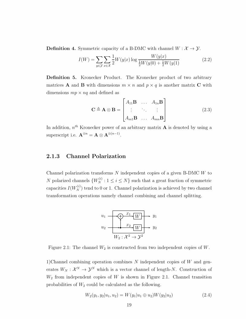
2.1.3 Channel Polarization
Channel polarization transforms N independent copies of a given B-DMC W to
N polarized channels {W (i)N : 1 ≤ i ≤ N} such that a great fraction of symmetric
capacities I(W(i)N ) tend to 0 or 1. Channel polarization is achieved by two channel
transformation operations namely channel combining and channel splitting.
u2
u1
b W
W
y2
y1
W2 : X 2 → Y2
x1
x2
Figure 2.1: The channel W2 is constructed from two independent copies of W .
1)Channel combining operation combines N independent copies of W and gen-
erates WN : XN → YN which is a vector channel of length-N . Construction of
W2 from independent copies of W is shown in Figure 2.1. Channel transition
probabilities of W2 could be calculated as the following.
W2(y1, y2|u1, u2) = W (y1|u1 ⊕ u2)W (y2|u2) (2.4)
19
2)Channel splitting operation splits the synthesized vector channel WN into N
binary-input DMC W(i)N : X → YN × X i−1. For length 2 vector channel W2,
one can produce two binary-input DMC i.e. W 12 : X → Y2 and W 2
2 : X →Y2 × X . Channel transition probabilities of W 1
2 and W 22 could be calculated as
the following.
W 12 (y1, y2|u1) =
∑
u2∈X
1
2W (y1|u1 ⊕ u2)W (y2|u2) (2.5)
W 22 (y1, y2, u1|u2) =
1
2W (y1|u1 ⊕ u2)W (y2|u2) (2.6)
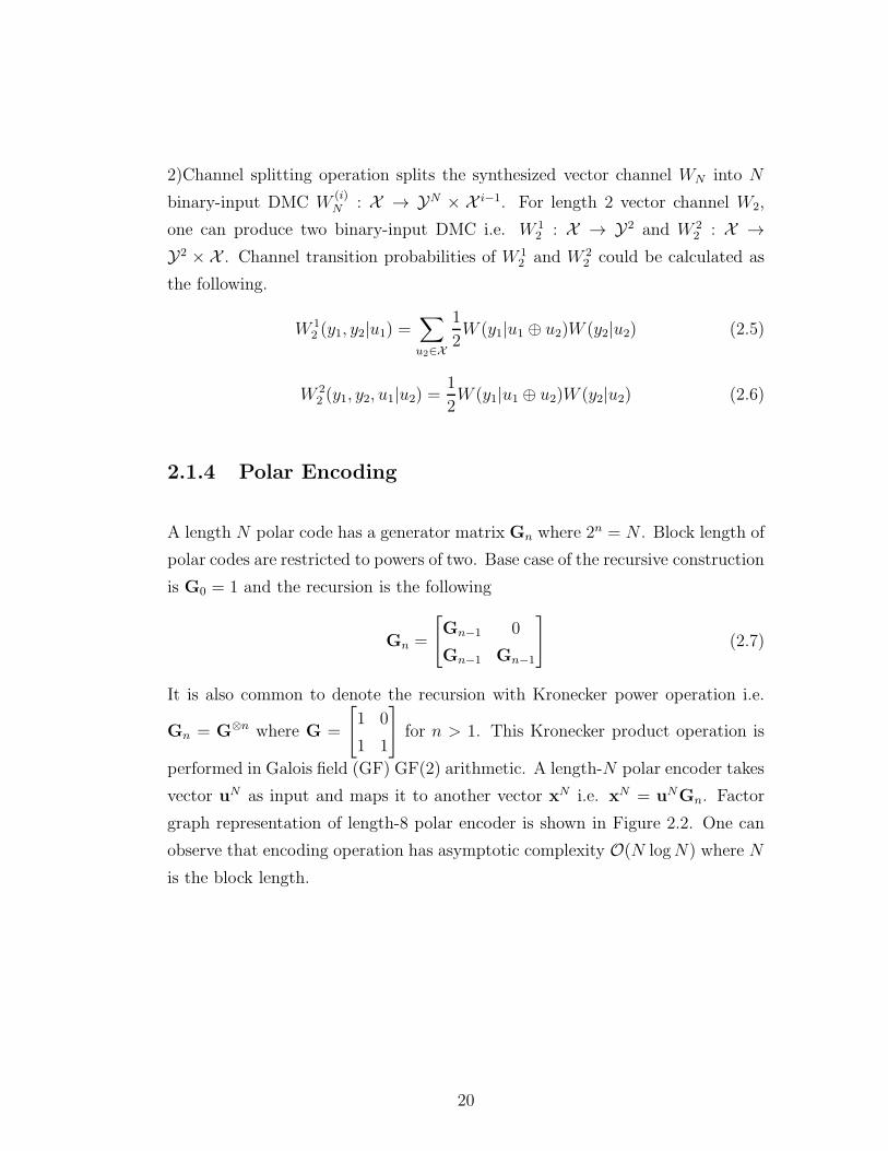
2.1.4 Polar Encoding
A length N polar code has a generator matrix Gn where 2n = N . Block length of
polar codes are restricted to powers of two. Base case of the recursive construction
is G0 = 1 and the recursion is the following
Gn =
[
Gn−1 0
Gn−1 Gn−1
]
(2.7)
It is also common to denote the recursion with Kronecker power operation i.e.
Gn = G⊗n where G =
[
1 0
1 1
]
for n > 1. This Kronecker product operation is
performed in Galois field (GF) GF(2) arithmetic. A length-N polar encoder takes
vector uN as input and maps it to another vector xN i.e. xN = uNGn. Factor
graph representation of length-8 polar encoder is shown in Figure 2.2. One can
observe that encoding operation has asymptotic complexity O(N logN) where N
is the block length.
20
u1
u2
u3
u4
u5
u6
u7
u8
x1
x2
x3
x4
x5
x6
x7
x8
b
b
b
b
b
b
b
b
b
b
b
b
Figure 2.2: Length 8 polar encoder.
21
2.1.5 Code Construction Methods
Aim of the polar code construction is the identification of A i.e. the set of free-bit
channels. For length-N and payload K polar code, K bit-channels with highest
capacity is included in the set A. Bit-channels in A will carry information with
rate one while bit-channels in Ac does not carry information. Thus, data to be
transmitted is inserted into uA sub-vector and remaining bit channels uAc are set
to a predetermined value. Calculation of bit-channel capacities I(W(i)N ) are chan-
nel dependent. Exact calculation for binary erasure channel (BEC) BEC(ǫ) is
derived in [37]. This calculation becomes infeasible when the channel is not BEC
due to exponential increase in the output alphabet proportional block length.
Density Evolution method [39] is used in LDPC code designs where several con-
volution operations are involved. Density Evolution method for polar codes is
described in [40] and [41], authors developed an algorithm that limits the output
alphabet size to compute bit-channel capacities.
2.1.6 Systematic Polar Coding
Systematic polar codes are introduced in [42]. BER performance of the polar
codes could be increased while preserving the complexity of encoding and de-
coding same as non-systematic polar coding. Consider the composition of polar
codeword x as in Equation 2.8 where set A is the indices of free-bit channel and
GA is the sub-matrix of G consisting of row indices in A.
x = uAGA + uAcGAc (2.8)
Now partition the polar codeword x = (xB,xBc) where B is an arbitrary subset of
indices. Equation 2.8 could be rewritten in terms of xB and xBc as in Equations
2.9 and 2.10 where GAB is a sub-matrix of G with elements Gi,j : i ∈ A, j ∈ B.We will set A = B to establish a one-to-one correspondence between uA and xB.
xB = uAGAB + uAcGAcB (2.9)
xBc = uAGABc + uAcGAcBc (2.10)
22
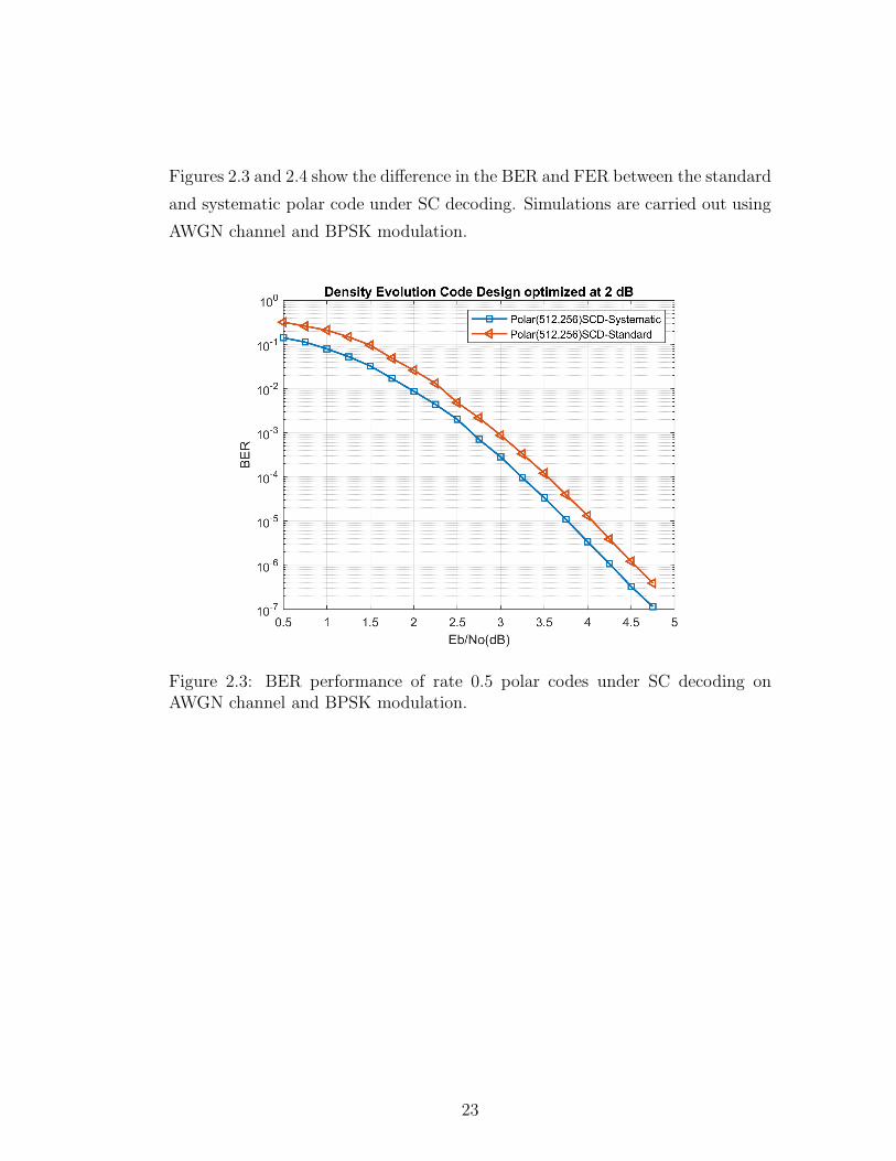
Figures 2.3 and 2.4 show the difference in the BER and FER between the standard
and systematic polar code under SC decoding. Simulations are carried out using
AWGN channel and BPSK modulation.
Figure 2.3: BER performance of rate 0.5 polar codes under SC decoding onAWGN channel and BPSK modulation.
23
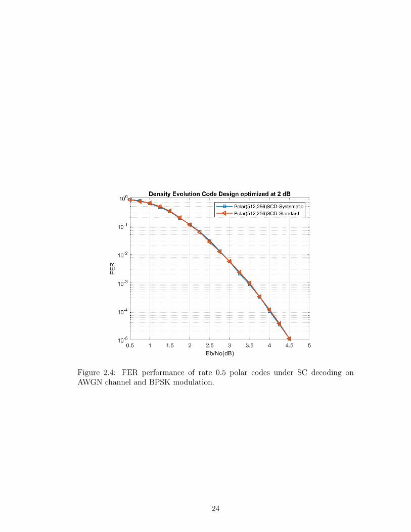
Figure 2.4: FER performance of rate 0.5 polar codes under SC decoding onAWGN channel and BPSK modulation.
24
2.1.7 Decoding Algorithms
Polar decoding algorithms are explained in this subsection. Successive cancella-
tion (SC) and successive cancellation list (SCL) algorithms are two well-known
polar decoding algorithms.
2.1.7.1 Successive Cancellation Decoding Algorithm
SC decoding algorithm is a depth-first search algorithm with asymptotic com-
plexity O(N logN) [37]. Data on the ith bit-channel is estimated using Equation
2.11. One can observe that decoding of ui depends on the previous bit channel
estimates. Thus, decoding takes place one by one from the first bit channel to
the last.
ui =
argmaxui= {W (yN , ui−1
1 |ui = 0),W (yN , ui−11 |ui = 1)} i ∈ A
0 i ∈ Ac(2.11)
We will use log-likelihood ratio (LLR) representation of the channel probabilities
as in Equation 2.12 where W (yi|xi) is the channel transition probability density
function. Decision LLRs are shown in Equation 2.13 where positive decision LLR
will be decoded as ui = 0 and negative decision LLR will be decoded as ui = 1.
ℓi = log
(
W (yi|xi = 0)
W (yi|xi = 1)
)
(2.12)
ℓi = log
(
W (yi, ui−11 |ui = 0)
W (yi, ui−11 |ui = 0)
)
(2.13)
SC decoder calculates the decision LLRs from channel LLRs using the update
Equations 2.14 and 2.15 [43] where ℓ denotes the LLR values and u ∈ {0, 1}.
f(ℓ1, ℓ2) = 2tanh−1
(
tanh(ℓ12)tanh(
ℓ22)
)
(2.14)
g(ℓ1, ℓ2, u) = (−1)uℓ1 + ℓ2 (2.15)
Equation 2.16 approximates Equation 2.14. We will refer to Equation 2.16 as
min-sum approximation of Equation 2.14.
f(ℓ1, ℓ2) ≈ sgn(ℓ1ℓ2)min(|ℓ1|, |ℓ2|) (2.16)
25
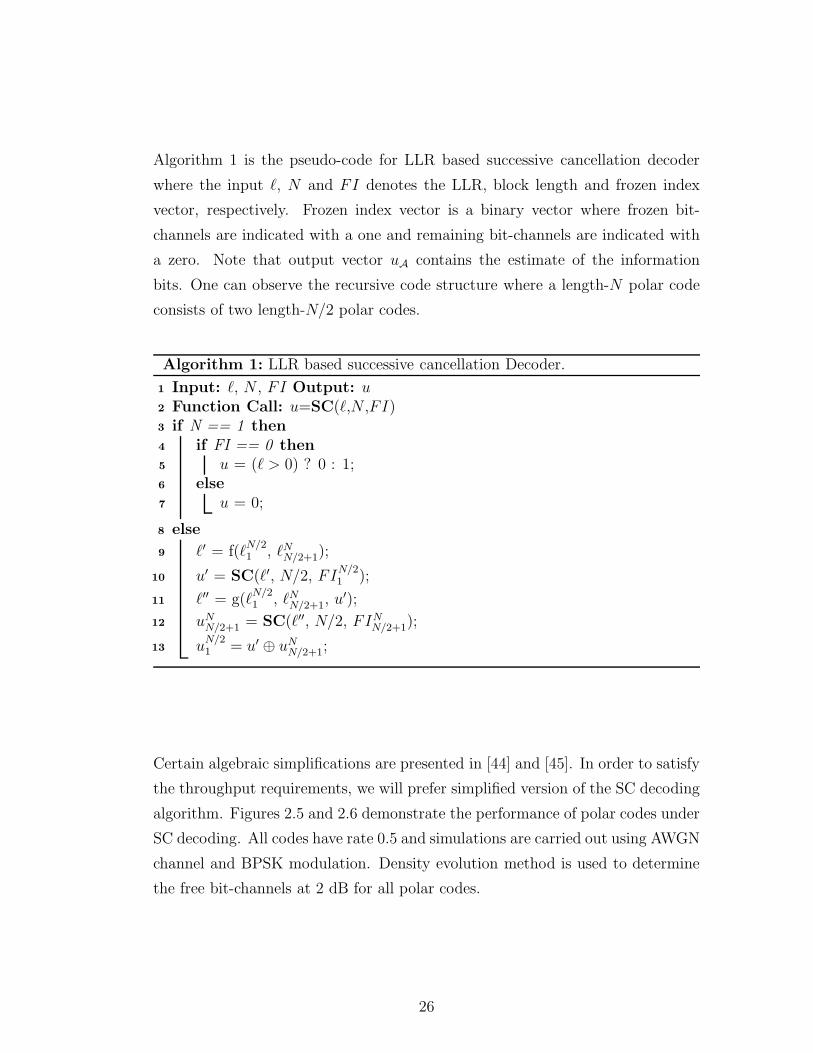
Algorithm 1 is the pseudo-code for LLR based successive cancellation decoder
where the input ℓ, N and FI denotes the LLR, block length and frozen index
vector, respectively. Frozen index vector is a binary vector where frozen bit-
channels are indicated with a one and remaining bit-channels are indicated with
a zero. Note that output vector uA contains the estimate of the information
bits. One can observe the recursive code structure where a length-N polar code
consists of two length-N/2 polar codes.
Algorithm 1: LLR based successive cancellation Decoder.
1 Input: ℓ, N , FI Output: u2 Function Call: u=SC(ℓ,N ,FI)3 if N == 1 then4 if FI == 0 then5 u = (ℓ > 0) ? 0 : 1;6 else7 u = 0;
8 else
9 ℓ′ = f(ℓN/21 , ℓNN/2+1);
10 u′ = SC(ℓ′, N/2, FIN/21 );
11 ℓ′′ = g(ℓN/21 , ℓNN/2+1, u
′);
12 uNN/2+1 = SC(ℓ′′, N/2, FINN/2+1);
13 uN/21 = u′ ⊕ uN
N/2+1;
Certain algebraic simplifications are presented in [44] and [45]. In order to satisfy
the throughput requirements, we will prefer simplified version of the SC decoding
algorithm. Figures 2.5 and 2.6 demonstrate the performance of polar codes under
SC decoding. All codes have rate 0.5 and simulations are carried out using AWGN
channel and BPSK modulation. Density evolution method is used to determine
the free bit-channels at 2 dB for all polar codes.
26
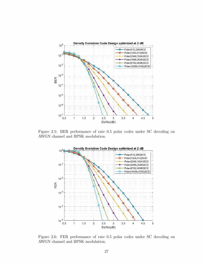
Figure 2.5: BER performance of rate 0.5 polar codes under SC decoding onAWGN channel and BPSK modulation.
Figure 2.6: FER performance of rate 0.5 polar codes under SC decoding onAWGN channel and BPSK modulation.
27
2.1.7.1.1 Area Estimation of SC Decoder An area estimation method-
ology of SC decoding algorithm with unrolled and pipelined architecture is pre-
sented in this part. This estimation should serve as a basis for the code designer
in assessment of the hardware complexity of the decoders without performing any
synthesis. Number of logic gates and memory elements required for the decoder is
calculated using software tools. We have expressed basic decoding functions de-
scribed in Section 2.1.7.1 with the help of [46] as logic gates. Number of pipeline
states is estimated as proportional to the total number of decoding operations. D-
type flip-flops (FFs) are used for memory elements. By using TSMC 28nm HPC
standard cell library, we have generated a data sheet of components and its area.
Two area estimates are generated one consisting of only drive-one components
and another consisting of mixture of drive-one to drive-eight components. Arith-
metic mean of these two estimates (Eavg) is reported as the final area estimate.
70% utilization is assumed for wire area. In [47], area of the Polar(1024,512)
code with unrolled and fully pipelined decoder is reported as 4.63 mm2 in 28nm
technology node. By using the developed methodology, area of the same decoder
is estimated as Eavg = 3.6 mm2 which is reasonably close.
2.1.7.2 Successive Cancellation List Decoding Algorithm
Successive cancellation list decoding algorithm is presented in [48]. Instead of
tracking a single path in the depth-first search, SCL algorithm keeps track of
L candidate codewords at any depth. This search method is known as the M-
Algorithm [49]. Candidate codewords are compared by a metric which is a sum-
mary of the decoding history of the codeword. LLR-based SCL algorithm is
presented in [50] where comparison metric simplifies to accumulation of contrast-
ing decisions. Equations 2.17 and 2.18 are used to calculate the path metric PMi
of a candidate codeword at depth i. Here ℓi and ui are the decision LLR and the
decision of the ith bit-channel, respectively.
PMi = φ(PMi−1, ℓi, ui) (2.17)
28
φ(PM, ℓ, u) =
PM u = 12(1− sgn(ℓ))
PM + |ℓ| u 6= 12(1− sgn(ℓ))
(2.18)
Asymptotic run-time complexity of the SCL algorithm is O(LNlgN) where L is
the list size and N is the block length. Complexity of path metric comparisons
is excluded in this notation. One can observe that, for sufficiently large list sizes,
comparison of path metrics between candidate codewords becomes the dominat-
ing factor for the decoding complexity. Algorithm 2 is the pseudo-code for LLR
based SCL decoder where index i is used for bit-channels, index j is used for lists
and L denotes the set of active decoding paths. Duplicate function appends the
input to itself in the column direction such that the output has twice the column
length of the input.
Algorithm 2: LLR based successive cancellation list decoder.
1 if i ∈ Ac then2 foreach ℓi,j ∈ L do3 PMi,j = φ(PMi−1,j, ℓi,j, ui);
4 ui,j = ui;
5 else6 Duplicate(PMi,L);7 foreach ℓj ∈ L do8 if j < |L|/2 then9 PMi,j = φ(PMi−1,j, ℓi,j, 0);
10 ui,j = 0;
11 else12 PMi,j = φ(PMi−1,j, ℓi,j, 1);13 ui,j = 1;
14 if |L| > ListSize then15 [ v,idx] = sort(PMi,j);16 PMi,j = vListSize1 ;17 ui,j = ui,idxListSize
1
;
18 L = LidxListSize1
;
Similar to SC decoding algorithm, certain algebraic simplifications are introduced
29
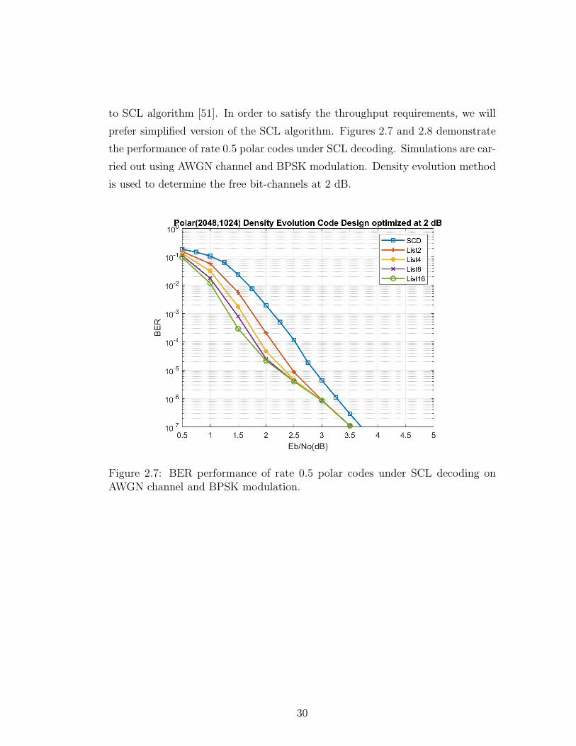
to SCL algorithm [51]. In order to satisfy the throughput requirements, we will
prefer simplified version of the SCL algorithm. Figures 2.7 and 2.8 demonstrate
the performance of rate 0.5 polar codes under SCL decoding. Simulations are car-
ried out using AWGN channel and BPSK modulation. Density evolution method
is used to determine the free bit-channels at 2 dB.
Figure 2.7: BER performance of rate 0.5 polar codes under SCL decoding onAWGN channel and BPSK modulation.
30
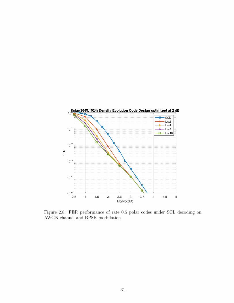
Figure 2.8: FER performance of rate 0.5 polar codes under SCL decoding onAWGN channel and BPSK modulation.
31
2.2 Reed-Solomon Codes
Reed-Solomon codes are described in [52]. This code becomes desirable when cor-
related binary errors or burst errors occur. An RS code is described as RSm(N ,K)
where m is the order of the finite Galois field GF(2m), N is the block length in
symbols and K is the payload in symbols. Note that GF(2m) contains 2m − 1
distinct elements, thus block length of the RS code is bounded by N ≤ 2m − 1.
RS codes exploit the maximum distance separable (MDS) property since they
achieve Singleton bound. An RSm(N ,K) code can correct up to 2t+ e ≤ N −K
error and erasure combinations where t is the number of errors and e is the num-
ber of erasures. For example, RS8(255,223) code is defined over GF(28) and can
correct up to 16 errors t ≤ 16 or 32 erasures e ≤ 32. This code is known as the
National Aeronautics and Space Administration (NASA) code which is used in
deep space communications.
2.2.1 Analytical Error Performance and Emulation Meth-
ods
Solid behavior of RS decoders allows performance estimation by analytical cal-
culations with negligible errors. In [53], authors derived the exact probability of
undetected error for a given RS code. Undetected errors occur if the received pat-
tern falls into the radius t Hamming sphere of another codeword in the codebook.
In Equation 2.19, PE(u) denotes the probability of undetected error event within
a distance u codeword (u > t), Du denotes the weight enumerator function of the
RS code and d = n − k + 1. PE(u) can become significantly large if t is small
compared to m.
PE(u) =Du
(
Nu
)
(m− 1)ud− t ≤ u ≤ N (2.19)
Keeping PE(u) in mind, BER characteristics of RS codes can be estimated for
given symbol error probability PSE. In Equation 2.20, PUE is the probability of
32
an uncorrectable symbol error.
PUE =
N∑
i=t+1
i
N
(
N
i
)
× (PSE)i × (1− PSE)
(N−i) (2.20)
Input and output BER of the RS decoder could be calculated by
BERin = 1− (1− PSE)1
m (2.21)
BERout = 1− (1− PUE)1
m (2.22)
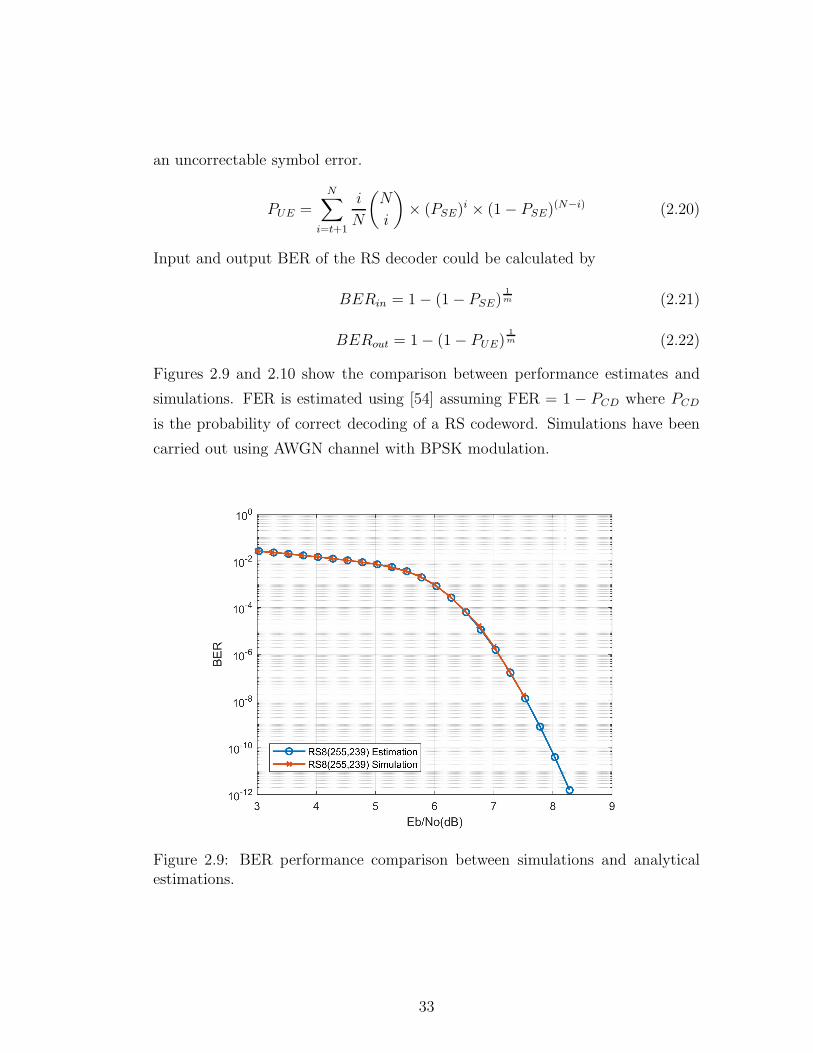
Figures 2.9 and 2.10 show the comparison between performance estimates and
simulations. FER is estimated using [54] assuming FER = 1 − PCD where PCD
is the probability of correct decoding of a RS codeword. Simulations have been
carried out using AWGN channel with BPSK modulation.
Figure 2.9: BER performance comparison between simulations and analyticalestimations.
33
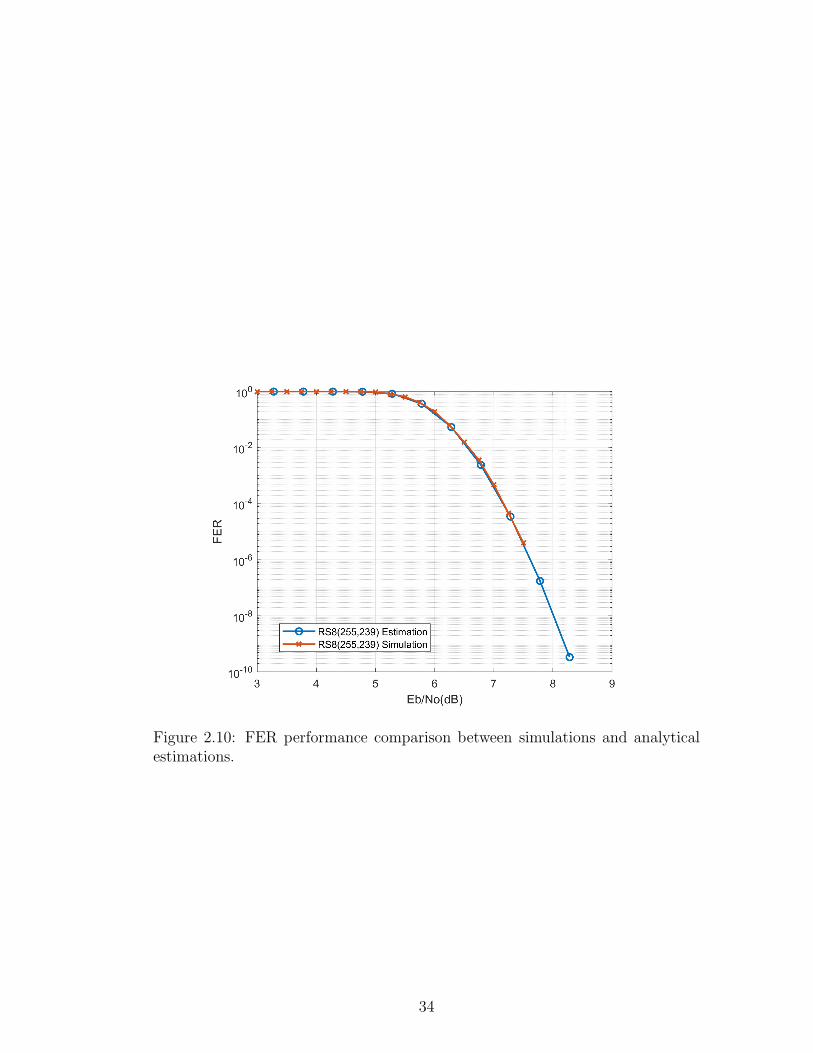
Figure 2.10: FER performance comparison between simulations and analyticalestimations.
34
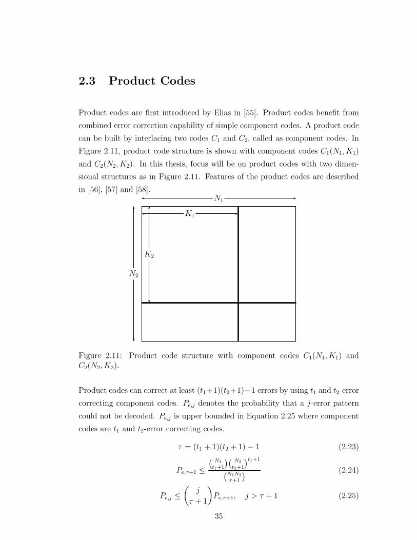
2.3 Product Codes
Product codes are first introduced by Elias in [55]. Product codes benefit from
combined error correction capability of simple component codes. A product code
can be built by interlacing two codes C1 and C2, called as component codes. In
Figure 2.11, product code structure is shown with component codes C1(N1, K1)
and C2(N2, K2). In this thesis, focus will be on product codes with two dimen-
sional structures as in Figure 2.11. Features of the product codes are described
in [56], [57] and [58].N1
N2
K2
K1
Figure 2.11: Product code structure with component codes C1(N1, K1) andC2(N2, K2).
Product codes can correct at least (t1+1)(t2+1)−1 errors by using t1 and t2-error
correcting component codes. Pe,j denotes the probability that a j-error pattern
could not be decoded. Pe,j is upper bounded in Equation 2.25 where component
codes are t1 and t2-error correcting codes.
τ = (t1 + 1)(t2 + 1)− 1 (2.23)
Pe,τ+1 ≤(
N1
t1+1
)(
N2
t2+1
)t1+1
(
N1N2
τ+1
) (2.24)
Pe,j ≤(
j
τ + 1
)
Pe,τ+1, j > τ + 1 (2.25)
35
2.4 Concatenated Codes
Concatenated codes are presented in [59] where long codes are built from shorter
ones. Aim of the concatenation is to combine the good parts of two codes to
diminish the weakness of the overall code. A concatenated FEC code consists of
at least two component codes. One of the codes could operate above the channel
capacity while the other code is operating near channel capacity in order to satisfy
the target coding rate. In the previous chapter, we have seen many concatenated
codes where soft and hard information is exchanged between codes. Concatenated
codes become favorable due to implementation constraints compared to longer
codes. In [60], authors have developed a concatenation scheme where polar and
RS codes are involved. Several RS codes operate on different parts of the multiple
polar blocks. A common concatenation for polar code is cyclic-redundancy-check
(CRC) when SCL algorithm is used to decode polar code [48].
2.5 Summary of the Chapter
A review of FEC codes are presented in this chapter including polar, RS, product
and concatenated codes. SC and SCL decoding algorithms are preferred for polar
codes. Density Evolution code construction along with systematic polar coding
is used to improve the BER performance. Analytical error performance and
emulation methods are used for RS code analysis. These codes will serve as a
basis to develop the polar product RS concatenated code.
36
Chapter 3
RS2-Polar Concatenation Scheme
Polar product RS (RS2-Polar) concatenation scheme is explained in this chapter.
Outer encoder and decoder pairs are described in Sections 3.1 and 3.4, respec-
tively. Interleaver and segmentation block is described in Section 3.2. Inner
encoder and decoder pairs are described in Section 3.3. Polar codes are used as
inner codes with rates slightly above the channel capacity. RS codes are used as
outer codes in a product form with rates closer to unity. Our aim is to collect the
soft information from the channel output as much as possible using polar codes.
Two-error correcting RS codes are used as component codes. We will present
code configurations with 28%, 24%, 20% and 15% overheads.
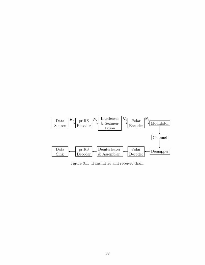
Figure 3.1 presents the transmitter and receiver blocks. Transmitter chain
begins with the product RS encoder and finishes with the modulator. Receiver
chain begins with the demapper and finishes with the product RS decoder. BPSK
modulation is used in simulations. Demapper calculates LLRs from channel out-
put. We have used the MDS property of RS codes to emulate the error correction
performance. In Figure 3.1, we denote the input and output of the outer en-
coder with Kr and Nr, respectively. We denote the input and output of the inner
encoder with Kp and Np, respectively.
37
DataSource
pr.RSEncoder
Interleaver& Segmen-
tation
PolarEncoder
Modulator
Channel
DemapperPolar
DecoderDeinterleaver& Assembler
pr.RSDecoder
DataSink
Kr Nr Kp Np
Figure 3.1: Transmitter and receiver chain.
38
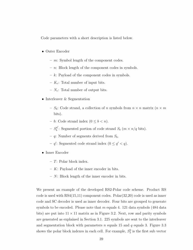
Code parameters with a short description is listed below.
• Outer Encoder
– m: Symbol length of the component codes.
– n: Block length of the component codes in symbols.
– k: Payload of the component codes in symbols.
– Kr: Total number of input bits.
– Nr: Total number of output bits.
• Interleaver & Segmentation
– Sb: Code strand, a collection of n symbols from n× n matrix (n×m
bits).
– b: Code strand index (0 ≤ b < n).
– Sq′
b : Segmented portion of code strand Sb (m× n/q bits).
– q: Number of segments derived from Sb.
– q′: Segmented code strand index (0 ≤ q′ < q).
• Inner Encoder
– T : Polar block index.
– K: Payload of the inner encoder in bits.
– N : Block length of the inner encoder in bits.
We present an example of the developed RS2-Polar code scheme. Product RS
code is used with RS4(15,11) component codes. Polar(32,20) code is used as inner
code and SC decoder is used as inner decoder. Four bits are grouped to generate
symbols to be encoded. Please note that m equals 4. 121 data symbols (484 data
bits) are put into 11× 11 matrix as in Figure 3.2. Next, row and parity symbols
are generated as explained in Section 3.1. 225 symbols are sent to the interleaver
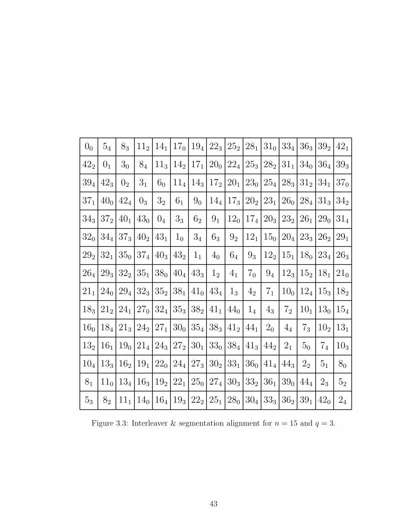
and segmentation block with parameters n equals 15 and q equals 3. Figure 3.3
shows the polar block indexes in each cell. For example, S02 is the first sub vector
39
the second code strand and could be calculated by applying Equations 3.1, 3.2
and 3.3. We begin with the calculation of S2 by using Equation 3.1.
S2 = {(0, 2), (1, 3), (2, 4), (3, 5), (4, 6), (5, 7), (6, 8), ..., (13, 0), (14, 1)}
Next, Equation 3.2 is used to align the starting index.
S2 = {(2, 4), (3, 5), (4, 6), (5, 7), (6, 8), ..., (13, 0), (14, 1), (0, 2), (1, 3)}
Finally, Equation 3.3 is used to split Sb into three equal pieces.
S02 = {(2, 4), (3, 5), (4, 6), (5, 7), (6, 8)}= {60, 61, 62, 63, 64}
Thus, first polar block encodes 1/3 of the diagonal which corresponds to 20 bits (5
symbols). Polar encoder is used 45 times to encode all symbols. 1440 coded bits
are generated by multiple use of polar encoder and sent to modulator. Modulated
symbols pass through AWGN channel. Inner decoder receives LLRs calculated by
demapper block. SC decoder calculates an estimate of the transmitted codeword
per received polar frame. SC decoder is used 45 times and 900 bits (225 symbols)
are sent to deinterleaver and assembler block. Received bits are formed into
groups of four bits to generate symbols. These symbols are placed into a 15 ×15 matrix as in Figure 3.3. Next, outer decoding operation begins with the
RS4(15,11) decoders in the horizontal direction and followed by the codes in the
vertical direction. After decoding on horizontal and vertical axes several times,
484 data bits are sent to data sink.
3.1 Outer Encoder
Outer encoder is explained in this section. Product RS encoder is used with two-
error correcting identical component codes on both axes. Figure 3.2 depicts the
product code structure where n is the block length of the component code and
k is the payload of the component code. Dashed lines indicate the position of
component codes in both dimensions. Cross hatched box indicates a collection
of m-bits. Kr bits are received by outer encoder and placed into k × k matrix.
40
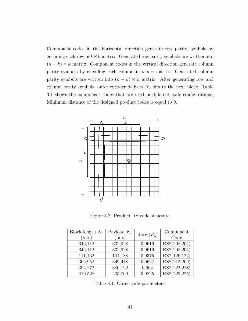
Component codes in the horizontal direction generate row parity symbols by
encoding each row in k×k matrix. Generated row parity symbols are written into
(n − k)× k matrix. Component codes in the vertical direction generate column
parity symbols by encoding each column in k × n matrix. Generated column
parity symbols are written into (n − k) × n matrix. After generating row and
column parity symbols, outer encoder delivers Nr bits to the next block. Table
3.1 shows the component codes that are used in different code configurations.
Minimum distance of the designed product codes is equal to 9.
nk
n
k
Figure 3.2: Product RS code structure.
Block-length Nr
(bits)Payload Kr
(bits)Rate (Ro)
ComponentCode
346,112 332,928 0.9619 RS8(208,204)346,112 332,928 0.9619 RS8(208,204)111,132 104,188 0.9375 RS7(126,122)362,952 349,448 0.9627 RS8(213,209)394,272 380,192 0.964 RS8(222,218)419,528 405,000 0.9825 RS8(229,225)
Table 3.1: Outer code parameters.
41
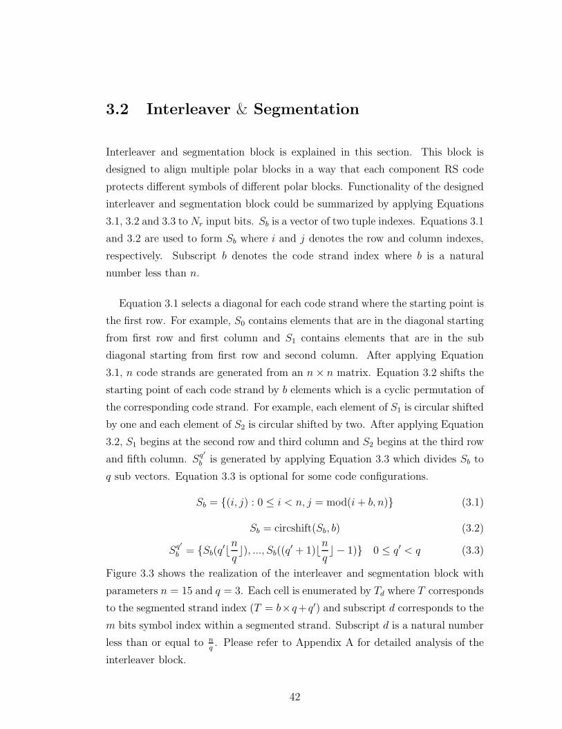
3.2 Interleaver & Segmentation
Interleaver and segmentation block is explained in this section. This block is
designed to align multiple polar blocks in a way that each component RS code
protects different symbols of different polar blocks. Functionality of the designed
interleaver and segmentation block could be summarized by applying Equations
3.1, 3.2 and 3.3 to Nr input bits. Sb is a vector of two tuple indexes. Equations 3.1
and 3.2 are used to form Sb where i and j denotes the row and column indexes,
respectively. Subscript b denotes the code strand index where b is a natural
number less than n.
Equation 3.1 selects a diagonal for each code strand where the starting point is
the first row. For example, S0 contains elements that are in the diagonal starting
from first row and first column and S1 contains elements that are in the sub
diagonal starting from first row and second column. After applying Equation
3.1, n code strands are generated from an n× n matrix. Equation 3.2 shifts the
starting point of each code strand by b elements which is a cyclic permutation of
the corresponding code strand. For example, each element of S1 is circular shifted
by one and each element of S2 is circular shifted by two. After applying Equation
3.2, S1 begins at the second row and third column and S2 begins at the third row
and fifth column. Sq′
b is generated by applying Equation 3.3 which divides Sb to
q sub vectors. Equation 3.3 is optional for some code configurations.
Sb = {(i, j) : 0 ≤ i < n, j = mod(i+ b, n)} (3.1)
Sb = circshift(Sb, b) (3.2)
Sq′
b = {Sb(q′⌊nq⌋), ..., Sb((q
′ + 1)⌊nq⌋ − 1)} 0 ≤ q′ < q (3.3)
Figure 3.3 shows the realization of the interleaver and segmentation block with
parameters n = 15 and q = 3. Each cell is enumerated by Td where T corresponds
to the segmented strand index (T = b×q+q′) and subscript d corresponds to the
m bits symbol index within a segmented strand. Subscript d is a natural number
less than or equal to nq. Please refer to Appendix A for detailed analysis of the
interleaver block.
42
00
01
02
03
04
10
11
12
13
14
20
21
22
23
24
30
31
32
33
34
40
41
42
43
44
50
51
52
53
54
60
61
62
63
64
70
71
72
73
74
80
81
82
83
84
90
91
92
93
94
100
101
102
103
104
110
111
112
113
114
120
121
122
123
124
130
131
132
133
134
140
141
142
143
144
150
151
152
153
154
160
161
162
163
164
170
171
172
173
174
180
181
182
183
184
190
191
192
193
194
200
201
202
203
204
210
211
212
213
214
220
221
222
223
224
230
231
232
233
234
240
241
242
243
244
250
251
252
253
254
260
261
262
263
264
270
271
272
273
274
280
281
282
283
284
290
291
292
293
294
300
301
302
303
304
310
311
312
313
314
320
321
322
323
324
330
331
332
333
334
340
341
342
343
344
350
351
352
353
354
360
361
362
363
364
370
371
372
373
374
380
381
382
383
384
390
391
392
393
394
400
401
402
403
404
410
411
412
413
414
420
421
422
423
424
430
431
432
433
434
440
441
442
443
444
Figure 3.3: Interleaver & segmentation alignment for n = 15 and q = 3.
43
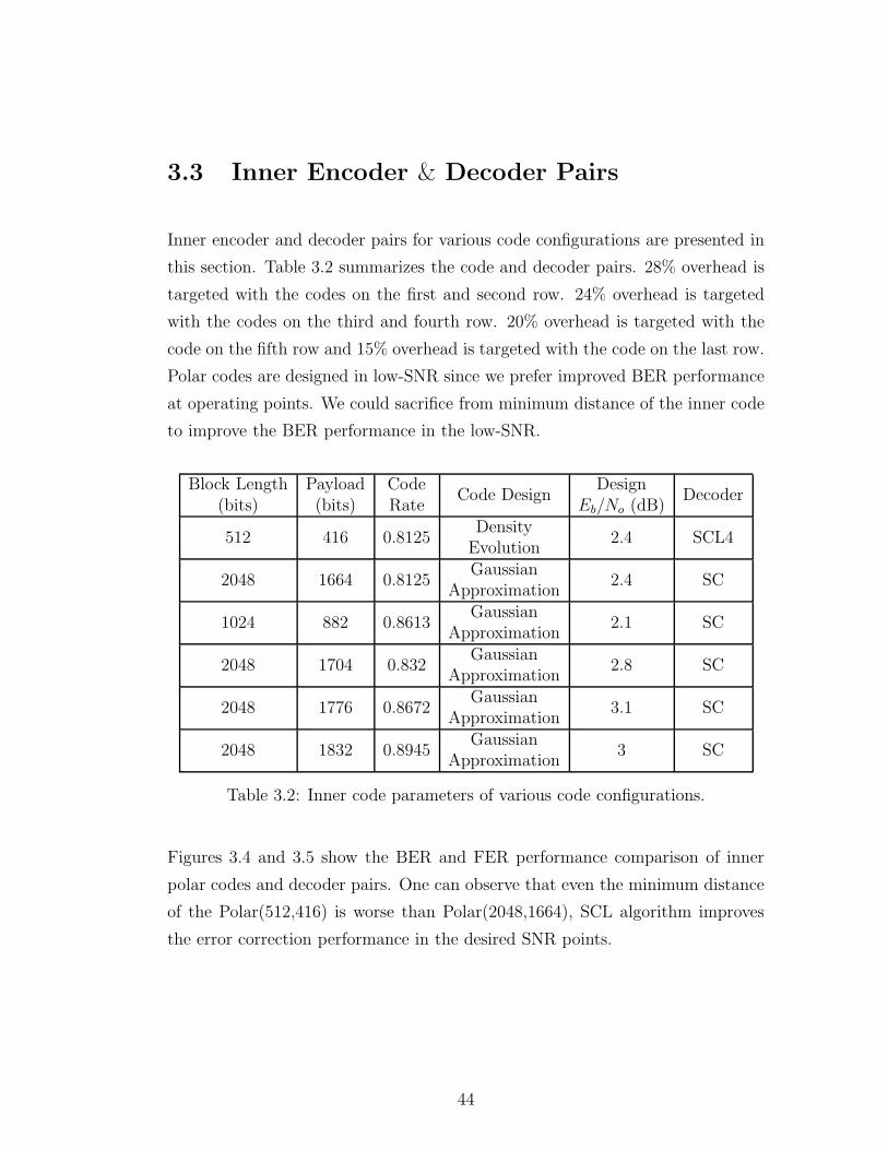
3.3 Inner Encoder & Decoder Pairs
Inner encoder and decoder pairs for various code configurations are presented in
this section. Table 3.2 summarizes the code and decoder pairs. 28% overhead is
targeted with the codes on the first and second row. 24% overhead is targeted
with the codes on the third and fourth row. 20% overhead is targeted with the
code on the fifth row and 15% overhead is targeted with the code on the last row.
Polar codes are designed in low-SNR since we prefer improved BER performance
at operating points. We could sacrifice from minimum distance of the inner code
to improve the BER performance in the low-SNR.
Block Length(bits)
Payload(bits)
CodeRate
Code DesignDesign
Eb/No (dB)Decoder
512 416 0.8125DensityEvolution
2.4 SCL4
2048 1664 0.8125Gaussian
Approximation2.4 SC
1024 882 0.8613Gaussian
Approximation2.1 SC
2048 1704 0.832Gaussian
Approximation2.8 SC
2048 1776 0.8672Gaussian
Approximation3.1 SC
2048 1832 0.8945Gaussian
Approximation3 SC
Table 3.2: Inner code parameters of various code configurations.
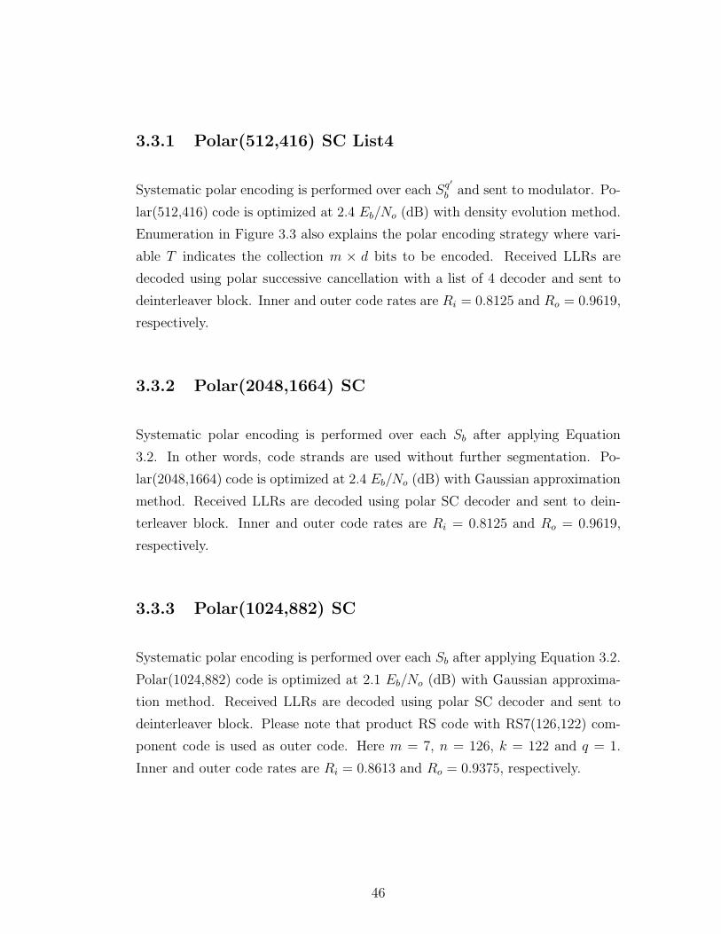
Figures 3.4 and 3.5 show the BER and FER performance comparison of inner
polar codes and decoder pairs. One can observe that even the minimum distance
of the Polar(512,416) is worse than Polar(2048,1664), SCL algorithm improves
the error correction performance in the desired SNR points.
44
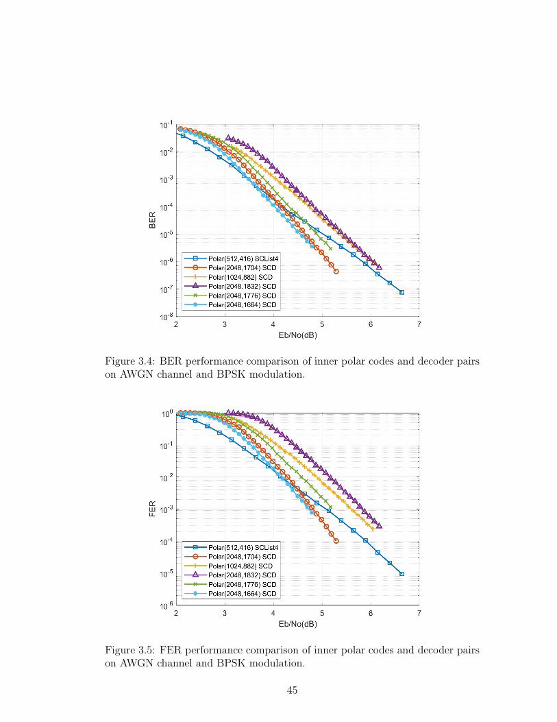
Figure 3.4: BER performance comparison of inner polar codes and decoder pairson AWGN channel and BPSK modulation.
Figure 3.5: FER performance comparison of inner polar codes and decoder pairson AWGN channel and BPSK modulation.
45
3.3.1 Polar(512,416) SC List4
Systematic polar encoding is performed over each Sq′
b and sent to modulator. Po-
lar(512,416) code is optimized at 2.4 Eb/No (dB) with density evolution method.
Enumeration in Figure 3.3 also explains the polar encoding strategy where vari-
able T indicates the collection m × d bits to be encoded. Received LLRs are
decoded using polar successive cancellation with a list of 4 decoder and sent to
deinterleaver block. Inner and outer code rates are Ri = 0.8125 and Ro = 0.9619,
respectively.
3.3.2 Polar(2048,1664) SC
Systematic polar encoding is performed over each Sb after applying Equation
3.2. In other words, code strands are used without further segmentation. Po-
lar(2048,1664) code is optimized at 2.4 Eb/No (dB) with Gaussian approximation
method. Received LLRs are decoded using polar SC decoder and sent to dein-
terleaver block. Inner and outer code rates are Ri = 0.8125 and Ro = 0.9619,
respectively.
3.3.3 Polar(1024,882) SC
Systematic polar encoding is performed over each Sb after applying Equation 3.2.
Polar(1024,882) code is optimized at 2.1 Eb/No (dB) with Gaussian approxima-
tion method. Received LLRs are decoded using polar SC decoder and sent to
deinterleaver block. Please note that product RS code with RS7(126,122) com-
ponent code is used as outer code. Here m = 7, n = 126, k = 122 and q = 1.
Inner and outer code rates are Ri = 0.8613 and Ro = 0.9375, respectively.
46
3.3.4 Polar(2048,1704) SC
Systematic polar encoding is performed over each Sb after applying Equation 3.2.
Polar(2048,1704) code is optimized at 2.8 Eb/No (dB) with Gaussian approxima-
tion method. Received LLRs are decoded using polar SC decoder and sent to
deinterleaver block. Please note that product RS code with RS8(213,209) com-
ponent code is used as outer code. Here m = 8, n = 213, k = 209 and q = 1.
Inner and outer code rates are Ri = 0.832 and Ro = 0.9627, respectively.
3.3.5 Polar(2048,1776) SC
Systematic polar encoding is performed over each Sb after applying Equation 3.2.
Polar(2048,1776) code is optimized at 3.1 Eb/No (dB) with Gaussian approxima-
tion method. Received LLRs are decoded using polar SC decoder and sent to
deinterleaver block. Please note that product RS code with RS8(222,218) com-
ponent code is used as outer code. Here m = 8, n = 222, k = 218 and q = 1.
Inner and outer code rates are Ri = 0.867 and Ro = 0.964, respectively.
3.3.6 Polar(2048,1832) SC
Systematic polar encoding is performed over each Sb after applying Equation 3.2.
Polar(2048,1832) code is optimized at 3 Eb/No (dB) with Gaussian approxima-
tion method. Received LLRs are decoded using polar SC decoder and sent to
deinterleaver block. Please note that product RS code with RS8(229,225) com-
ponent code is used as outer code. Here m = 8, n = 229, k = 225 and q = 1.
Inner and outer code rates are Ri = 0.8945 and Ro = 0.9653, respectively.
47
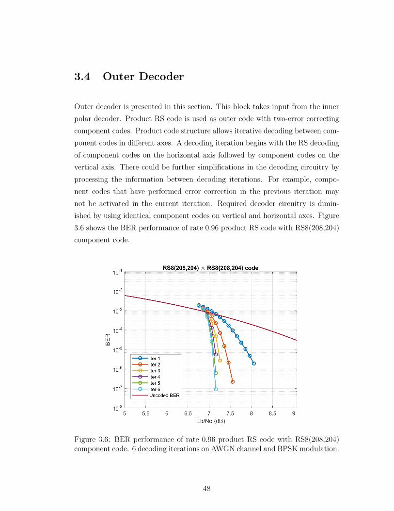
3.4 Outer Decoder
Outer decoder is presented in this section. This block takes input from the inner
polar decoder. Product RS code is used as outer code with two-error correcting
component codes. Product code structure allows iterative decoding between com-
ponent codes in different axes. A decoding iteration begins with the RS decoding
of component codes on the horizontal axis followed by component codes on the
vertical axis. There could be further simplifications in the decoding circuitry by
processing the information between decoding iterations. For example, compo-
nent codes that have performed error correction in the previous iteration may
not be activated in the current iteration. Required decoder circuitry is dimin-
ished by using identical component codes on vertical and horizontal axes. Figure
3.6 shows the BER performance of rate 0.96 product RS code with RS8(208,204)
component code.
Figure 3.6: BER performance of rate 0.96 product RS code with RS8(208,204)component code. 6 decoding iterations on AWGN channel and BPSK modulation.
48
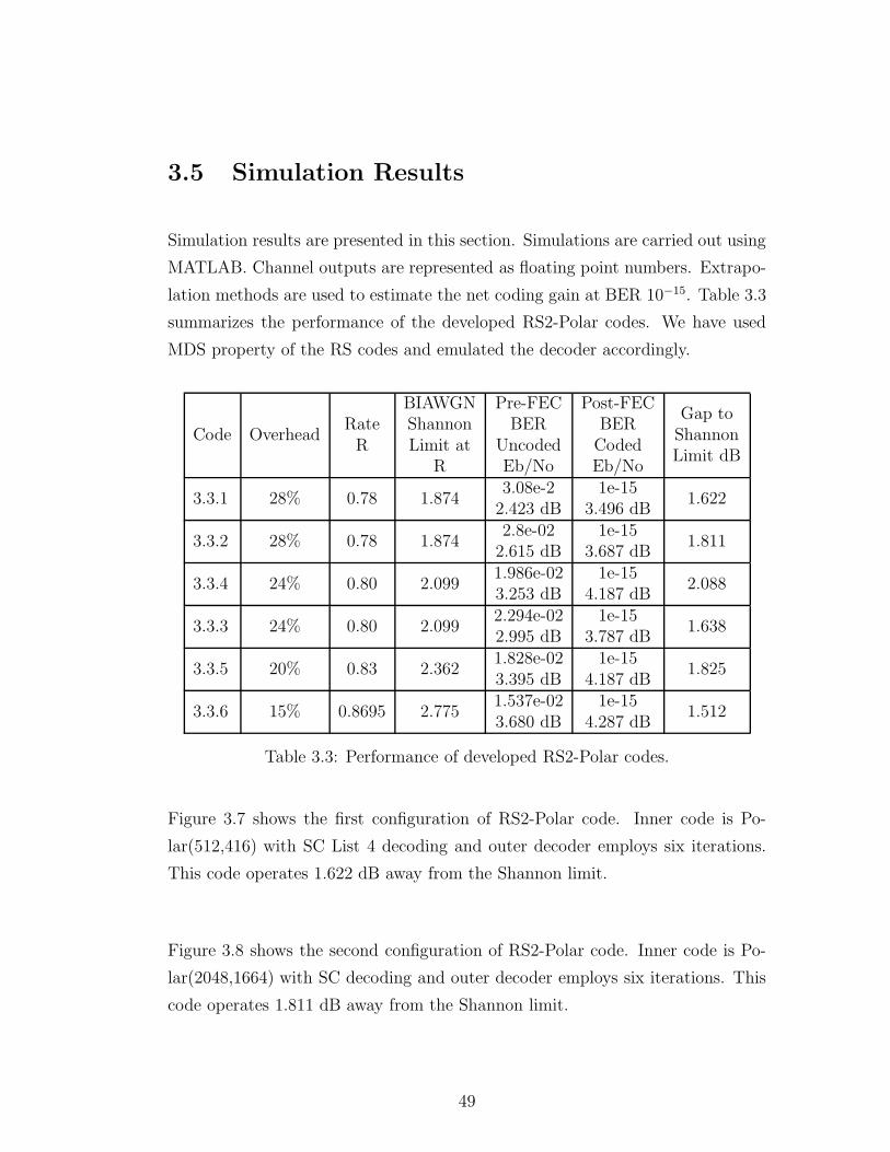
3.5 Simulation Results
Simulation results are presented in this section. Simulations are carried out using
MATLAB. Channel outputs are represented as floating point numbers. Extrapo-
lation methods are used to estimate the net coding gain at BER 10−15. Table 3.3
summarizes the performance of the developed RS2-Polar codes. We have used
MDS property of the RS codes and emulated the decoder accordingly.
Code OverheadRateR
BIAWGNShannonLimit at
R
Pre-FECBER
UncodedEb/No
Post-FECBERCodedEb/No
Gap toShannonLimit dB
3.3.1 28% 0.78 1.8743.08e-22.423 dB
1e-153.496 dB
1.622
3.3.2 28% 0.78 1.8742.8e-022.615 dB
1e-153.687 dB
1.811
3.3.4 24% 0.80 2.0991.986e-023.253 dB
1e-154.187 dB
2.088
3.3.3 24% 0.80 2.0992.294e-022.995 dB
1e-153.787 dB
1.638
3.3.5 20% 0.83 2.3621.828e-023.395 dB
1e-154.187 dB
1.825
3.3.6 15% 0.8695 2.7751.537e-023.680 dB
1e-154.287 dB
1.512
Table 3.3: Performance of developed RS2-Polar codes.
Figure 3.7 shows the first configuration of RS2-Polar code. Inner code is Po-
lar(512,416) with SC List 4 decoding and outer decoder employs six iterations.
This code operates 1.622 dB away from the Shannon limit.
Figure 3.8 shows the second configuration of RS2-Polar code. Inner code is Po-
lar(2048,1664) with SC decoding and outer decoder employs six iterations. This
code operates 1.811 dB away from the Shannon limit.
49
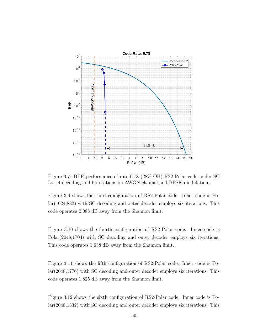
Figure 3.7: BER performance of rate 0.78 (28% OH) RS2-Polar code under SCList 4 decoding and 6 iterations on AWGN channel and BPSK modulation.
Figure 3.9 shows the third configuration of RS2-Polar code. Inner code is Po-
lar(1024,882) with SC decoding and outer decoder employs six iterations. This
code operates 2.088 dB away from the Shannon limit.
Figure 3.10 shows the fourth configuration of RS2-Polar code. Inner code is
Polar(2048,1704) with SC decoding and outer decoder employs six iterations.
This code operates 1.638 dB away from the Shannon limit.
Figure 3.11 shows the fifth configuration of RS2-Polar code. Inner code is Po-
lar(2048,1776) with SC decoding and outer decoder employs six iterations. This
code operates 1.825 dB away from the Shannon limit.
Figure 3.12 shows the sixth configuration of RS2-Polar code. Inner code is Po-
lar(2048,1832) with SC decoding and outer decoder employs six iterations. This
50
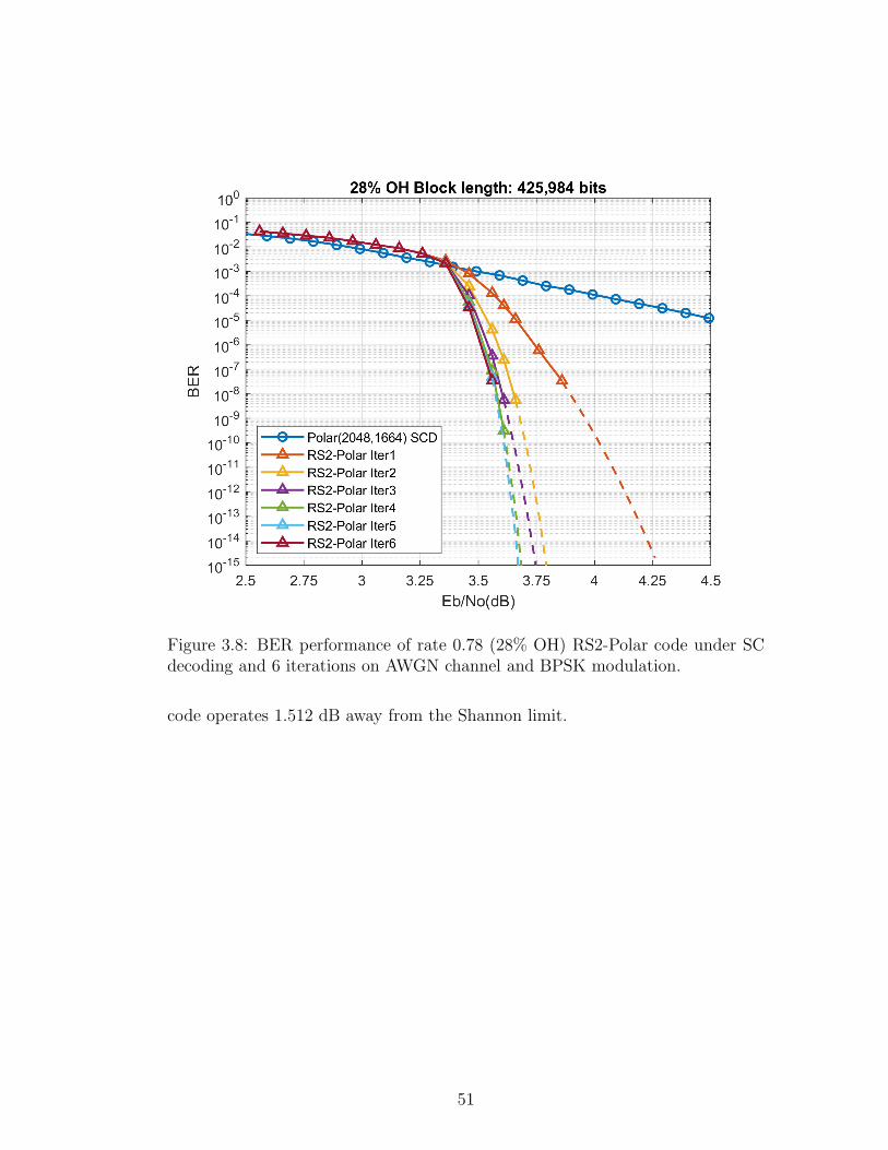
Figure 3.8: BER performance of rate 0.78 (28% OH) RS2-Polar code under SCdecoding and 6 iterations on AWGN channel and BPSK modulation.
code operates 1.512 dB away from the Shannon limit.
51
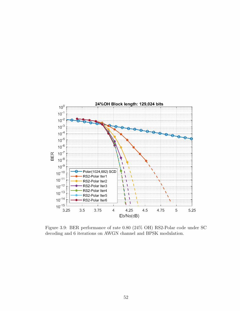
Figure 3.9: BER performance of rate 0.80 (24% OH) RS2-Polar code under SCdecoding and 6 iterations on AWGN channel and BPSK modulation.
52
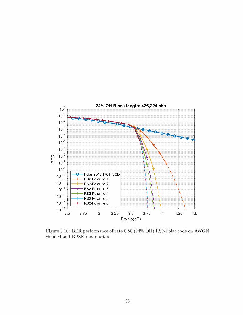
Figure 3.10: BER performance of rate 0.80 (24% OH) RS2-Polar code on AWGNchannel and BPSK modulation.
53
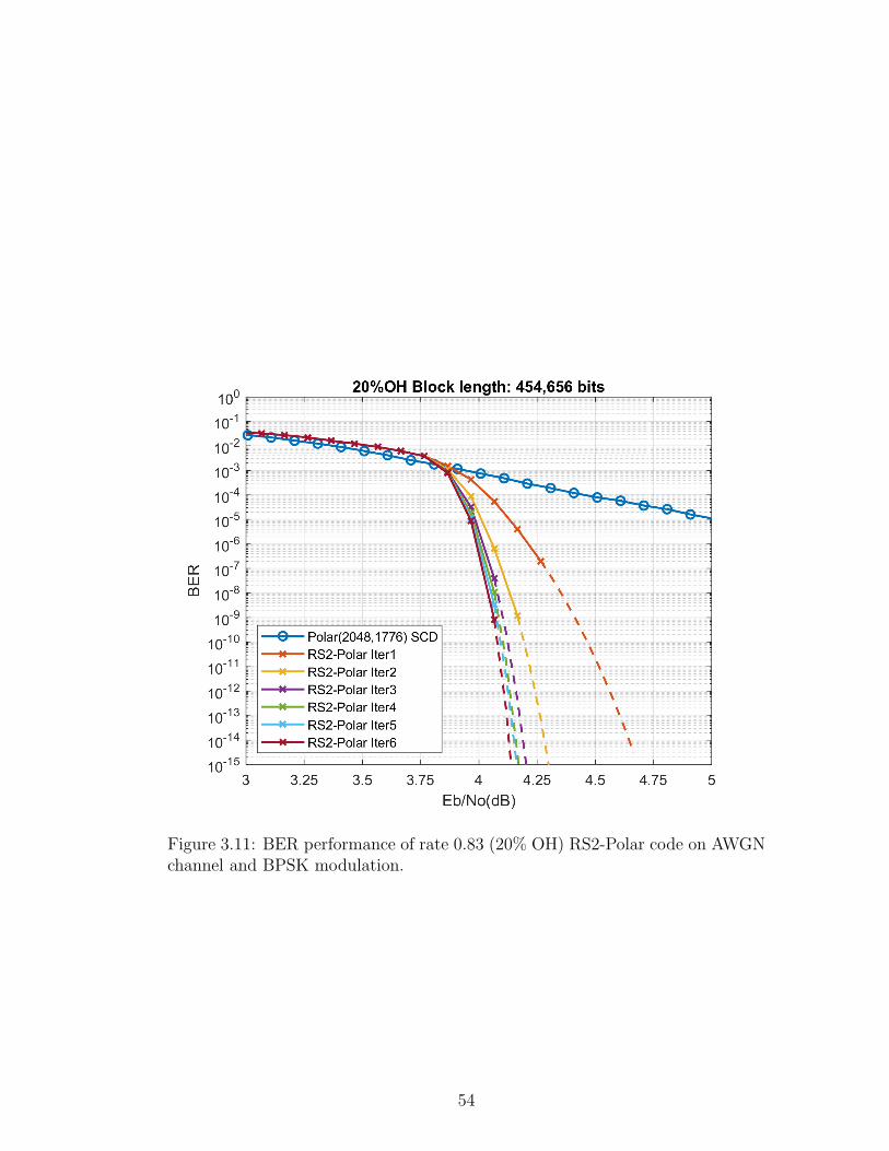
Figure 3.11: BER performance of rate 0.83 (20% OH) RS2-Polar code on AWGNchannel and BPSK modulation.
54
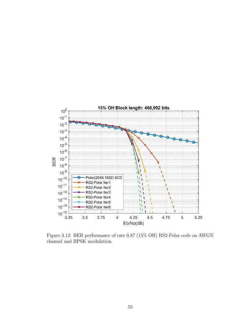
Figure 3.12: BER performance of rate 0.87 (15% OH) RS2-Polar code on AWGNchannel and BPSK modulation.
55
Simulation results show that there is a diminishing return in the number of
iterations where performance of 5 and 6 iterations may be negligible in some
applications.
Gap to Shannon limit of the developed codes are higher than the codes in the
literature since we have sacrificed from code complexity to satisfy the throughput
requirements. Performance of the developed code could be increased by using
soft information in a more efficient but costly way. First, SC decoder could be
replaced with SCL decoder or more complex decoders. This will reduce the BER
further at the expense of higher decoding complexity. Second, soft information
collected from channel output could be reused by the polar decoder. By sending
the information of corrected bits to inner code, polar decoder could override pre-
vious bit estimates and generate a better estimate of the transmitted codeword.
However, second method is more complex since it requires storage of the LLRs
and extra hardware to recalculate an estimate. In this thesis, we have used in-
ner and outer codes as building blocks without introducing any modifications to
satisfy the targets of the thesis.
3.6 Complexity Analysis
Complexity of the designed codes is analyzed in this section. Polar and RS
decoders are the two components of the developed algorithm. Algorithms have
been selected along with corresponding architectural templates considering EPIC
project targets. We will assess the complexity of the polar decoders by counting
the number of operations to decode the codeword. We will consider simplifications
on the GF multipliers in RS decoders. In [61], authors show that polar coding
is feasible at Tb/s throughput. In this thesis, we will consider similar block
lengths and corresponding architectural templates to support Tb/s throughput.
RS codes on GF(28) become favorable for two reasons (i) in [62], authors showed
the simplified version of multiplier architectures for GF(24n), (ii) code rate of
the product code could be selected in the desired range for t = 2 RS codes.
Complexity of the RS codes with low t is dominated by syndrome calculation
56
and Chien search. Chien search [63] could be skipped for t = 2 which reduces the
complexity of the decoder significantly. We refer [64] for details of the complexity
of the high-speed RS decoders.
3.6.1 Hardware Complexity
Hardware complexity of the decoder is analyzed in this subsection. We have
estimated the area of unrolled and pipelined polar decoder using the methodology
described in Section 2.1.7.1.1. We have synthesized Polar(2048,1664) SC decoder
in Genus and estimated 4.36 mm2 area from the netlist. Table 3.4 shows the
area estimates of the SC decoders by using the methodology described in Section
2.1.7.1.1.
Code (N,K) # of Steps Area(mm2)(2048,1704) 268 4.05(2048,1664) 277 4.07(2048,1776) 214 3.39(2048,1832) 187 3.13
Table 3.4: Area estimates of various polar SC decoders.
Figure 3.13 shows the hierarchical floor-planning of the RS2-Polar decoder with
Polar(2048,1664) inner code. We have synthesized the interleaver block in Ca-
dence and estimated 3.27 mm2 area from the netlist. We refer to [64] for the
detailed analysis of high-speed product RS codes where area occupation of the
product RS decoder is estimated as 6.63 mm2. Total area of the decoder is 14.27
mm2 in 28nm technology node. We have designed a core area with 1 × 2 ratio
(2.73 mm×5.234 mm). Input and output pins are placed to the top and bottom
of the chip, respectively. Number of input pins are 10240 where 5 bits of LLR
precision is used. Number of output pins are 3264. Area scaling methods are
used to estimate the area occupation of the decoder circuitry in 16nm. By using
Dennard’s scaling law [36], area of the decoder is estimated as 4.65 mm2 in 16nm.
57
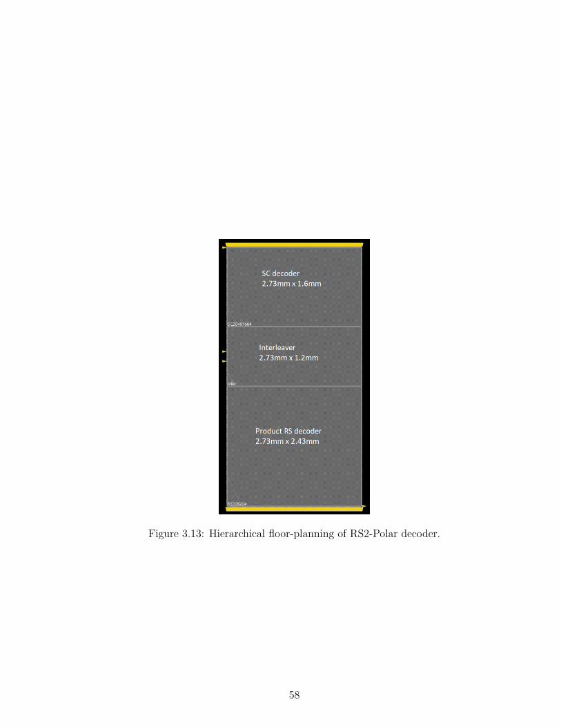
Figure 3.13: Hierarchical floor-planning of RS2-Polar decoder.
58
Required clock frequency fc = 626 MHz could be calculated using Equation
3.4 where W is the bus-width, γ is the throughput, Q is the LLR precision, R is
the code rate.
fc =γ
W
Q
R(3.4)
In advanced technology nodes (7/16/28nm), clock rates up to 1 GHz are identified
as feasible in [65]. Therefore, by sacrificing fromW , we kept fc within the feasible
range. Moreover, in EPIC project, 1024 block-length polar decoder is synthesized
successfully with 1.2 GHz clock frequency to support 1 Tb/s throughput. Inter-
leaver block could keep pace with polar decoder since it is much simpler than the
polar decoder. Simplicity of the t = 2 component RS decoders allow product RS
decoder to operate in the desired clock speed as well [64].
3.7 Comparison with Other Codes
Developed FEC decoder is compared with other decoders in terms of decoding
complexity and hardware complexity as much as possible. In [60], authors in-
terleaved polar and RS codes where the polar block protects the first symbol of
each RS codeword and so on. In this configuration, polar decoders work in par-
allel. After each polar decoder decodes a symbol, RS decoding takes place. After
corrections are done by RS codes, polar decoders continue to decode the next
symbol. Reusing soft information at the polar decoder is the major advantage of
this algorithm. There are two drawbacks of this design; (i) throughput require-
ments may not be satisfied since unrolled and pipelined polar decoder architecture
is not suitable for interlacing RS codes and (ii) high storage requirements due to
reusing soft information.
In [66] and [67], author shows that thousand bits block-length LDPC codes
with 3-4 iterations are feasible to support 1 Tb/s throughput. In [24], proposed
LDPC-BCH code is decoded with 32 iterations and block length equals to 38400
bits. It will not be practical to implement 32 iterations at 1 Tb/s throughput
due to hardware complexity limits.
59
In [27], authors developed a coding scheme that targets 1 Tb/s throughput.
Decoder complexity is relatively simpler than the RS2-Polar decoder. Area oc-
cupied is in the same order as the RS2-Polar decoder. Utilizing a hard decision
decoder limits the communications performance which could be a drawback of
the algorithm. Communications performance of this algorithm falls behind the
developed code in this thesis.
In [30], author designed polar codes with similar block-lengths to developed
RS2-Polar code. However, hardware complexity of this decoder is not feasible to
support the throughput requirements.
In [35], authors developed a turbo product code that can achieve 100 Gbps
throughput. The proposed design occupies 4.49 mm2 area with 1 GHz clock
frequency in 28nm technology. However, proposed decoder architecture is not
fully pipelined, thus increasing the throughput further may not be feasible due
to clock frequency limits.
3.8 Summary of the Chapter
RS2-Polar coding scheme is explained in this chapter. A specific interleaver is
developed to align inner and outer codes. Simulations have been carried out
to verify the communications performance of the developed coding scheme. We
have analyzed five code configurations which exhibit best performance among
other candidates. Hardware complexity of the developed decoder is analyzed by
projecting achieved results in the literature. Total area of the decoder is estimated
as 14.27 mm2 in 28nm technology. In 16nm technology, area of the decoder is
expected to be 4.65 mm2. Our estimations show that all the targets are satisfied
in 16nm technology node. Comparisons with other works in the literature show
that only the simplest algorithms could meet the complexity requirements while
supporting 1 Tb/s throughput. Although the developed codes do not exhibit the
best communication performance, it could support 1 Tb/s throughput under low
complexity decoding algorithms.
60
Chapter 4
Conclusion
A FEC code and architecture is developed that supports 1 Tb/s throughput for
optical communications. We have used combinations of simple codes to achieve
better performance with limited complexity. Polar codes are used as inner codes
and RS codes are used as outer codes in product form. Simulation results show
that developed FEC code achieves 11.5 dB net coding gain with 28% overhead.
Inner code is systematic Polar(512,416) under SC List 4 decoding. Outer code
is a product RS code with RS8(208,204) component codes. An interleaver is
developed to align the polar frames into product structure such that each byte
of a polar frame is protected by a different component code. Iterations between
inner and outer codes are not allowed to ensure a steady dataflow. We have
demonstrated that 1 Tb/s throughput is feasible by using the existing codes
without doing any modifications. Under these constraints, we have developed a
coding scheme which combines best features of two codes.
In Chapter 1, a comprehensive survey of FEC codes is presented that has
developed for optical communications. Most of the codes exploit reasonable com-
munications performance while supporting 100 Gb/s or more. Three evaluation
metrics are identified as error correction performance, decoding complexity and
area occupation. Area occupation and throughput requirements are adopted from
61
EPIC project targets. We have extended these targets and included communi-
cations performance to evaluation metrics. 10 mm2 area occupation, 1 Tb/s
throughput with reasonable net coding gain (> 10.5 dB) at 10−15 post-FEC BER
are selected as KPIs. Please note that these targets are only for decoder circuitry
in advanced technology nodes (7/16/28nm). In addition, polar encoding is quite
simple where only a series of XOR operations are involved.
In Chapter 2, a review of FEC codes are presented where polar, RS, product
and concatenated codes are included. SC and SCL decoding algorithms are pre-
ferred for decoding of polar codes. Extreme throughput requirement has limited
the code block-length and decoder complexity. Area occupation of the polar SC
decoder is estimated by calculating the area of each component in the gate level.
We have compared our area estimate with the codes that are implemented in the
literature. We conclude that our estimates are accurate enough to get an idea
without performing any synthesis.
In Chapter 3, RS2-Polar concatenation scheme is explained including inner
codes, outer codes and interleaver block. In the design stage, we have selected
rate of the inner code to be slightly above the channel capacity to collect soft
information as much as possible. Table 4.1 summarizes the achieved code perfor-
mances at 10−15 post-FEC BER where the first column denotes the corresponding
section number. All the codes satisfy the net coding gain requirement. Number
of iterations is set to six for all codes. Although there is a diminishing return
in the number of iterations to code performance, at least four iterations are nec-
essary to achieve a high coding gain. Simulation results show that inner code
design affects the code performance dramatically where codes on the first and
second row have different inner polar codes with the same overhead. On the
other hand, code on the first row utilizes a more complex decoder than the code
on the second row. Decoder complexity analysis shows that, a simple algorithm is
preferred for polar codes and there are further algorithmic simplifications in the
RS decoders. Instead of computation dominant architectures, we have preferred
memory dominant architectures to support 1 Tb/s throughput.
62
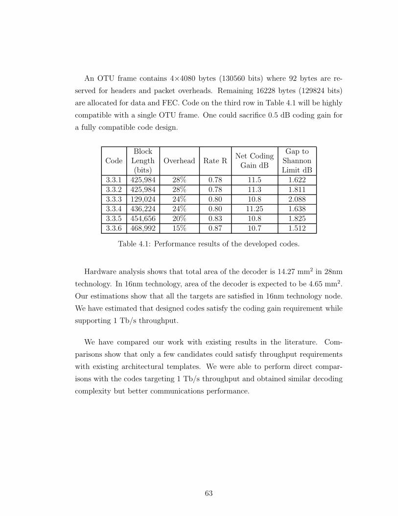
An OTU frame contains 4×4080 bytes (130560 bits) where 92 bytes are re-
served for headers and packet overheads. Remaining 16228 bytes (129824 bits)
are allocated for data and FEC. Code on the third row in Table 4.1 will be highly
compatible with a single OTU frame. One could sacrifice 0.5 dB coding gain for
a fully compatible code design.
CodeBlockLength(bits)
Overhead Rate RNet CodingGain dB
Gap toShannonLimit dB
3.3.1 425,984 28% 0.78 11.5 1.6223.3.2 425,984 28% 0.78 11.3 1.8113.3.3 129,024 24% 0.80 10.8 2.0883.3.4 436,224 24% 0.80 11.25 1.6383.3.5 454,656 20% 0.83 10.8 1.8253.3.6 468,992 15% 0.87 10.7 1.512
Table 4.1: Performance results of the developed codes.
Hardware analysis shows that total area of the decoder is 14.27 mm2 in 28nm
technology. In 16nm technology, area of the decoder is expected to be 4.65 mm2.
Our estimations show that all the targets are satisfied in 16nm technology node.
We have estimated that designed codes satisfy the coding gain requirement while
supporting 1 Tb/s throughput.
We have compared our work with existing results in the literature. Com-
parisons show that only a few candidates could satisfy throughput requirements
with existing architectural templates. We were able to perform direct compar-
isons with the codes targeting 1 Tb/s throughput and obtained similar decoding
complexity but better communications performance.
63
Bibliography
[1] C. E. Shannon, “A Mathematical Theory of Communication,” The Bell Sys-
tem Technical Journal, vol. 27, pp. 379–423, Jul 1948.
[2] Y. Polyanskiy, H. V. Poor, and S. Verdu, “Channel Coding Rate in the Finite
Blocklength Regime,” IEEE Transactions on Information Theory, vol. 56,
May 2010.
[3] M. C. Coskun, G. Durisi, T. Jerkovits, G. Liva, W. Ryan, B. Stein,
and F. Steiner, “Efficient Error-Correcting Codes in the Short Blocklength
Regime,” Physical Communication, vol. 34, pp. 66–79, 2019.
[4] E. Agrell, M. Karlsson, A. R. Chraplyvy, D. J. Richardson, P. M. Krumm-
rich, and P. Winzer, “Roadmap of optical communications,” Journal of Op-
tics, vol. 18, no. 6, 2016.
[5] ITU, G.709 Interfaces for the optical transport network. ITU, Nov 2019.
[6] I. C. Society, IEEE Standard for Ethernet, 2015.
[7] I. C. Society, Physical Layers and Management Parameters for 50 Gb/s, 200
Gb/s and 400 Gb/s Operations over Single-Mode Fiber, Nov 2019.
[8] S. Bjornstad, “Can OTN be replaced by Ethernet?,” 22nd Conference on
Optical Network Design and Modelling, 2018.
[9] P. Larsson-Edefors, C. Foughstedt, and K. Cushon, “Implementation Chal-
lenges for Energy Efficient Error Correction in Optical Communication Sys-
tems,” Advanced Photonic Congress, 2018.
64
[10] K. Szczerba, C. Fougstedt, P. Larsson-Edefors, P. Westbergh, A. G. i Amat,
L. Svensson, M. Karlsson, A. Larsson, and P. A. Andrekson, “Impact of
Forward Error Correction on Energy Consumption of VCSEL-Based Trans-
mitters,” European Conference on Optical Communication (ECOC), 2015.
[11] ITU, G.975 Forward Error Correction for Submarine Systems, Oct 2000.
[12] C. Kestel, M. Herrmann, and N. Wehn, “When Channel Coding Hits the
Implementation Wall,” 2018 IEEE 10th International Symposium on Turbo
Codes and Iterative Information Processing (ISTC), Dec 2018.
[13] EPIC, “Enabling Practical Wireless Tb/s Communications with Next Gen-
eration Channel Coding.” H2020, 2020.
[14] ITU, G.975.1 Forward Error Correction for High Bit-Rate DWDM Subma-
rine Systems, Feb 2004.
[15] R. G. Gallager, “Low-Density Parity-Check Codes,” IRE Transactions on
Information Theory, vol. 8, pp. 21–28, Jan 1962.
[16] R. C. Bose and D. K. R. Chaudhuri, “On A Class of Error Correcting Binary
Group Codes,” Information and Control, vol. 3, pp. 68–79, 1960.
[17] B. P. Smith, A. Farhood, A. Hunt, F. R. Kschischang, and J. Lodge, “Stair-
case Codes: FEC for 100 Gb/s OTN,” Journal of Lightwave Technology,
vol. 30, Jan 2012.
[18] OIF, 100G Forward Error Correction White Paper, May 2010.
[19] B. P. Smith and F. R. Kschischang, “Future Prospects for FEC in Fiber-
Optic Communications,” IEEE Journal of Selected Topics in Quantum Elec-
tronics, vol. 16, pp. 1245–1257, Sep 2010.
[20] A. Sheikh, A. G. i Amat, G. Liva, C. Hager, and H. D. Pfister, “On Low-
Complexity Decoding of Product Codes for High-Throughput Fiber-Optic
Systems,” 2018 IEEE 10th International Symposium on Turbo Codes and
Iterative Information Processing, Dec 2018.
65
[21] A. Sheikhand, A. G. i Amat, and G. Liva, “Iterative Bounded Distance De-
coding of Product Codeswith Scaled Reliability,” 2018 European Conference
on Optical Communication (ECOC), Nov 2018.
[22] T. Ahmad, “Polar Codes for Optical Communications,” Master’s thesis,
Bilkent University, May 2016.
[23] G. Tzimpragos, C. Kachris, I. B. Djordjevic, M. Cvijetic, D. Soudris, and
I. Tomkos, “A Survey on FEC Codes for 100 G and Beyond Optical Net-
works,” IEEE Communication Surveys and Tutorials, vol. 18, first quarter
2016.
[24] K. Sugihara, Y. Miyata, T. Sugihara, K. Kubo, H. Yoshida, W. Matsumoto,
and T. Mizuochi, “A Spatially-coupled Type LDPC Code with an NGC
of 12 dB for Optical Transmission beyond 100Gb/s,” 2013 Optical Fiber
Communication Conference and Exposition and the National Fiber Optic
Engineers Conference (OFC/NFOEC), June 2013.
[25] D. Chang, F. Yu, Z. Xiao, N. Stojanovic, F. N. Hauske, Y. Cai, C. Xie, L. Li,
X. Xu, and Q. Xiong, “LDPC convolutional codes using layered decoding
algorithm for high speed coherent optical transmission,” OFC/NFOEC, May
2012.
[26] L. M. Zhang and F. R. Kschischang, “Low-Complexity Soft-Decision Con-
catenated LDGM-Staircase FEC for High-Bit-Rate Fiber-Optic Communica-
tion,” IEEE Journal of Lightwave Technology, vol. 35, no. 18, pp. 3991–3999,
2017.
[27] C. Foughstedt and P. Larsson-Edefors, “Energy-Efficient High-Throughput
VLSI Architectures for Product-Like Codes,” Journal of Lightwave Technol-
ogy, vol. 37, Jan 2019.
[28] C. Foughstedt, A. Sheikhand, A. G. i Amat, G. Liva, and P. Larsson-Edefors,
“Energy-Efficient Soft-Assisted Product Decoders,” 2019 Optical Fiber Com-
munications Conference and Exhibition (OFC), Apr 2019.
[29] M. Barakatain and F. R. Kschischang, “Low-Complexity Concatenated
LDPC-Staircase codes,” Journal of Lightwave Technology, vol. 36, Jun 2018.
66
[30] T. Ahmad and F. Khan, “On the Coding Gain of Polar Codes for High
Speed Communications over AWGN Channels,” 17th International Bhurban
Conference on Applied Sciences and Technology (IBCAST), Jan 2020.
[31] C. Condo, P. Giard, F. Leduc-Primeau, G. Sarkis, and W. J. Gross, “A 9.52
dB NCG FEC Scheme and 162 b/Cycle Low-Complexity Product Decoder
Architecture,” IEEE Transactions on Circuits and Systems-I, vol. 65, Apr
2018.
[32] Y. Miyata, K. Kubo, K. Sugihara, T. Ichikawa, W. Matsumoto, H. Yoshida,
and T. Mizuochi, “Performance Improvement of a Triple-Concatenated FEC
by a UEP-BCH Product Code for 100 Gb/s Optical Transport Networks,”
18th OptoElectronics and Communications Conference (OECC), 2013.
[33] S. I. Han, J. P. Fonseka, and E. M. Dowling, “Constrained Turbo Block
Convolutional Codes for 100G and Beyond Optical Transmissions,” IEEE
Photonics Technology Letters, vol. 26, May 2014.
[34] V. Inc., ECC66100 Series SD-FEC Encoder/Decoder Cores, 2017.
[35] Y. Wang, J. Lin, and Z. Wang, “A 100 Gbps Turbo Product Code Decoder
for Optical Communications,” 2019 IEEE 5th International Conference on
Computer and Communications, pp. 721–725, Dec 2019.
[36] R. H. Dennard, F. H. Gaensslen, H.-N. Yu, V. L. Rideout, E. Bassous,
and A. L. Leblanc, “Design of Ion-Implanted MOSFET’s with Very Small
Physical Dimensions,” IEEE Journal of Solid-State Circuits, vol. 9, Oct 1974.
[37] E. Arikan, “Channel Polarization: A Method for Constructing Capacity-
Achieving Codes for Symmetric Binary-Input Memoryless Channels,” IEEE
Transactions on Information Theory, vol. 55, pp. 3051–3073, Jul 2009.
[38] 3GPP, “5G NR Channel Coding and Multiplexing,” tech. rep., ETSI, 2018.
[39] T. Richardson and R. Urbanke, Modern Coding Theory. Cambridge Univer-
sity Press, 2008.
[40] P. Trifonov, “Efficient Design and Decoding of Polar Codes,” IEEE Trans-
actions on Communications, vol. 60, pp. 3221–3227, Nov 2012.
67
[41] I. Tal and A. Vardy, “How to Construct Polar Codes,” IEEE Transactions
on Information Theory, vol. 59, pp. 6562–6582, Oct 2013.
[42] E. Arikan, “Systematic Polar Coding,” IEEE Communications Letters,
vol. 15, pp. 860–862, Aug 2011.
[43] W. E. Ryan and S. Lin, Channel Codes: Classical and Modern. Cambridge
University Press, 2009.
[44] A. Alamdar-Yazdi and F. R. Kschischang, “A Simplified Successive-
Cancellation Decoder for Polar Codes,” IEEE Communications Letters,
vol. 15, pp. 1378–1380, Dec 2011.
[45] G. Sarkis, P. Giard, A. Vardy, C. Thibeault, and W. J. Gross, “Fast Polar
Decoders: Algorithm and Implementation,” IEEE Journal on Selected Areas
in Communications, vol. 32, pp. 946–957, May 2014.
[46] C. Zhang, B. Yuan, and K. K. Parhi, “Reduced-latency SC Polar Decoder
Architectures,” 2012 IEEE International Conference on Communications,
Jun 2012.
[47] P. Giard, C. Thibeault, and W. J. Gross, High-Speed Decoders for Polar
Codes. Springer, 2017.
[48] I. Tal and A. Vardy, “List Decoding of Polar Codes,” IEEE Transactions on
Information Theory, vol. 61, pp. 2213–2226, May 2015.
[49] J. B. Anderson and S. Mohan, “Sequential Coding Algorithms: A Survey and
Cost Analysis,” IEEE Transactions on Communications, vol. 32, pp. 169–
176, Feb 1984.
[50] A. Balatsoukas-Stimming, M. B. Parizi, and A. Burg, “LLR-Based Succes-
sive Cancellation List Decoding of Polar Codes,” IEEE Transactions on Sig-
nal Processing, vol. 63, pp. 5165–5179, Oct 2015.
[51] S. A. Hashemi, C. Condo, and W. J. Gross, “Fast Simplified Successive-
Cancellation List Decoding of Polar Codes,” 2017 IEEE Wireless Commu-
nications and Networking Conference Workshops (WCNCW), May 2017.
68
[52] I. S. Reed and G. Solomon, “Polynomial Codes Over Certain Finite Fields,”
J. Soc. Indust. Appl. Math., vol. 8, Jun 1960.
[53] K.-M. Cheung and R. J. McEliece, “The Undetected Error Probability
for Reed-Solomon Codes,” Military Communications Conference, vol. 1,
pp. 163–167, Oct 1988.
[54] T. C. Nolan and W. E. Stark, “A Recursive Method for Calculating Error
Probabilities for a Reed-Solomon Codeword,” VTC’98. 48th IEEE Vehicular
Technology Conference. Pathway to Global Wireless Revolution, pp. 1613–
1617, May 1998.
[55] P. Elias, “Error-Free Coding,” IRE Transactions Information Theory, 1954.
[56] N. Abramson, “Cascade Decoding of Cyclic Product Codes,” IEEE Trans-
actions on Communications Technology, vol. 16, pp. 398–402, June 1968.
[57] S. M. Reddy and J. P. Robinson, “Random Error and Burst Correction
by Iterated Codes,” IEEE Transactions on Information Theory, vol. IT-18,
January 1972.
[58] F. Blomqvist, “On Hard-Decision Decoding of Product Codes.”
https://arxiv.org/abs/2001.04715, 2020.
[59] G. D. Forney, “Concatenated Codes,” MIT Technical Report, December
1965.
[60] H. Mahdavifar, M. El-Khamy, and I. Kang, “Performance Limits and Prac-
tical Decoding of Interleaved Reed-Solomon Polar Concatenated Codes,”
IEEE Transactions on Communications, vol. 62, May 2014.
[61] A. Sural, E. G. Sezer, Y. Ertugrul, O. Arikan, and E. Arikan, “Terabits-per-
Second Throughput for Polar Codes,” 2019 IEEE 30th International Sym-
posium on Personal, Indoor and Mobile Radio Communications (PIMRC
Workshops), Oct 2019.
[62] C. Paar, P. Fleischmann, and P. Roelse, “Efficient Multiplier Architectures
for Galois Fields gf(2sup4n),” IEEE Transactions on Computers, vol. 47,
Feb 1998.
69
[63] R. Chien, “Cyclic Decoding Procedures for Bose- Chaudhuri-Hocquenghem
Codes,” IEEE Transactions on Information Theory, vol. 10, pp. 357–363,
Oct 1964.
[64] E. G. Sezer, “ASIC Implementation Study of Reed-Solomon Codes.” private
communication, 2020.
[65] EPIC, “D1.2 B5G Wireless Tb/s FEC KPI Requirement and Technology
Gap Analysis,” tech. rep., H2020, 2018.
[66] N. Wehn, “High Throughput Coding: An Implementation Centric View,”
oct 2019.
[67] Channel Coding for Tbit/s Communications: An Implementation Centric
View, Zenodo, oct 2019.
70
Appendix A
Interleaver
Interleaver block is analyzed in this chapter. Interleaver is designed in such a way
that a component RS code protects distinct m bits of distinct polar blocks. This
property could be satisfied by using component codes with odd block lengths.
We will prove this property for 0th m bit collection of polar block since the rest
will be trivial.
Lemma. Let x and y to be two distinct even numbers in [α, 2α) interval. Let
x′ = mod(α) and y′ = mod(α) where α is an odd number. Then x′ and y′ are
distinct odd numbers.
Proof. Use Euclidean division to represent x and y in terms of α, x′ and y′.
x = cα + x′ and y = cα + y′ where x′ 6= y′ since x 6= y. Since α is odd, x′ and y′
must be odd.
Let component code block length equal to 2n+1, (i, j) denote an element of
interleaver matrix and T0 denote the set of locations of 0th m bit collection of each
polar block. First m bit collection of the polar blocks will occupy the following
indexes.
T0 = {(0, 0), (1, 2), (2, 4), ..., (2n− 2, 4n− 4), (2n− 1, 4n− 2), (2n, 4n)} (A.1)
More precisely mod(2n+1) will be applied to each element of T0 to find the
71

location in (2n + 1)× (2n + 1) matrix. Here index i of each element remain the
same since all of them are less than 2n+1. Index j becomes the following.
T0 = {(0, 0), (1, 2), (2, 4), ..., (2n−2, 2n−5), (2n−1, 2n−3), (2n, 2n−1)} (A.2)
One can observe that index j of the each element in T0 is a distinct number in
[0, 2n − 1) interval since in A.1 index j’s less than 2n+1 are all even numbers
and index j’s greater than 2n+1 will become distinct odd numbers since Lemma.
Therefore, 0th m bit collection of each polar block will be on different rows and
columns. This property could be generalized to other elements in the interleaver
matrix.
For component codes with even block lengths this property could not be sat-
isfied in vertical axis since mod(2n) of even numbers are also even numbers.
72