Polynomial Lower Bounds for theTwo-Machine Flowshop Problem withSequence-Independent Setup Times

Anis Gharbi 1,2, Talel Ladhari 1,3

Princess Fatimah Alnijris’s Research Chair for AMT

Department of Industrial Engineering

College of Engineering, King Saud University, Riyadh, Saudi Arabia

Mohamed Kais Msakni 4

Combinatorial Optimization Research Group – ROI

Ecole polytechnique de Tunisie, BP 743, 2078 La Marsa, Tunisia

Mehdi Serairi 5

Heudiasyc UMR 6599, Centre de Recherches de Royallieu

Universit de Technologie de Compiegne

France

Abstract

In this paper, we address the problem of two-machine flowshop scheduling problemwith sequence independent setup times to minimize the total completion time. Wepropose five new polynomial lower bounds. Computational results based on ran-domly generated data show that our proposed lower bounds consistently outperformthose of the literature.

Keywords: Flowshop, setup times, total completion time, lower bounds

Electronic Notes in Discrete Mathematics 36 (2010) 1089–1096

1571-0653/$ – see front matter © 2010 Elsevier B.V. All rights reserved.

www.elsevier.com/locate/endm

doi:10.1016/j.endm.2010.05.138

1 Introduction

We consider the strongly NP-hard scheduling problem of minimizing the totalcompletion time on a two-machine permutation flowshop with setup times(denoted by F2 | STsi |

∑Cj). As soon as a machine Mi(i = 1, 2) becomes

available, a job j(j = 1, ..., n) requires a sequence-independent setup time si,jbefore being processed for pi,j units of time on that machine. An interestingdatabase Internet connectivity application of the F2|STsi

∑Cj can be found

in [1].

Bagga and Khurana [3] were the first to address the F2|STsi|∑

Cj prob-lem. They proposed two lower bounds, a dominance rule and a branch-and-bound algorithm which could only solve small-sized instances with up to 9jobs. Allahverdi [2] implemented the lower bounds of [3], together with twonew dominance rules in a branch-and-bound algorithm which was able to solveinstances with up to 35 jobs. Moreover, he proposed three constructive heuris-tics which have been combined with local search procedures by Al-Anzi andAllahverdi [1]. These heuristics have been recently outperformed by those ofMsakni et al. [5] who also proposed a genetic local search algorithm that pro-vides near-optimal solutions in reasonable CPU time for large-sized instanceswith up to 500 jobs.

In the sequel, we briefly describe the lower bounds of Bagga and Khu-rana [3]. Then, we introduce new lower bounds for the F2|STsi|

∑Cj and

provide computational results which show the good performance of the pro-posed lower bounds.

2 Lower bounds of Bagga and Khurana [3]

In this section, we describe the two lower bounds of Bagga and Khurana [3],denoted hereafter by LB1 and LB2. To the best of our knowledge, these arethe only available lower bounds for F2 | STsi |

∑Cj.

If we relax the capacity of the second machine, then we get a single machineproblem 1 | sj , qj |

∑Cj with setup times sj = s1,j and tails qj = p2,j

(j = 1, ..., n). The optimal total completion time of the obtained problem is

1 Dr. Anis Gharbi and Dr. Talel Ladhari would like to thank Princess Fatimah Alnijris’sResearch Chair for Advanced Manufacturing Technology for the provided financial support.2 Email: a.gharbi@ksu.edu.sa3 Email: talel ladhari2004@yahoo.fr4 Email: msakni kais@yahoo.fr5 Email: mehdi.serairi@hds.utc.fr

A. Gharbi et al. / Electronic Notes in Discrete Mathematics 36 (2010) 1089–10961090

a valid lower bound for F2 | STsi |∑

Cj. Let C1j denote the completion time

of job j in the SPT (optimal) sequence of the 1 ||∑

Cj problem which isobtained after merging the setup time and the processing time of each job.We have LB1 =

∑n

j=1C1j +

∑n

j=1 qj .

In the computation of LB2, it is assumed that s1,j = p1,j = 0. Consequently,a single machine problem 1 | sj |

∑Cj with setup times sj = s2,j (j = 1, ..., n)

is obtained. Then, LB2 is equal to the corresponding optimal total completiontime which is obtained using the SPT rule after merging the setup time andthe processing time of each job.

LB1 and LB2 can be computed in O(n logn) time.

3 New waiting time-based lower bounds

Let δj (j = 1, ..., n) denote the minimum amount of time that a job j has towait between its exit from M1 and its starting time on M2. Clearly, a validlower bound for F2 | STsi |

∑Cj is LBWT =

∑n

j=1C1j +

∑n

j=1 p2,j +∑n

j=1 δj .

In this section, we focus on deriving effective lower bounds on the totalwaiting time Δ =

∑n

j=1 δj . Note that trivially setting δj = 0 for all j = 1, ..., nyields the lower bound LB1 of Bagga and Khurana [3]. Therefore, all the lowerbounds which are proposed in this section dominate LB1.

3.1 A zero predecessor-based lower bound

M2

M1p1,j

p2,j

δ1j

s1,j p1,j

s2,j p2,j

δ1j = 0

s1,j

s2,jM2

M1

Case (i) Case (ii)

Fig. 1. Illustration of δ1j computation

It is worth noting that the setup operation of each job j on M2 startsat least at the same time as its setup operation on M1. Two cases are to beconsidered (see figure 1):

(i) s2,j ≤ s1,j + p1,j : job j will start processing on M2 immmediately afterits completion on M1. That is, δj = 0.

(ii) s2,j > s1,j + p1,j : job j has to wait until M2 is prepared to process it.In this case, we have δj = s2,j − s1,j − p1,j.

A. Gharbi et al. / Electronic Notes in Discrete Mathematics 36 (2010) 1089–1096 1091

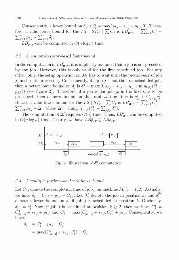
Consequently, a lower bound on δj is δ1j = max(s2,j − s1,j − p1,j, 0). There-

fore, a valid lower bound for the F2 | STsi |∑

Cj is LB1WT =

∑n

j=1C1j +∑n

j=1 p2,j +∑n

j=1 δ1j .

LB1WT can be computed in O(n logn) time.

3.2 A one predecessor-based lower bound

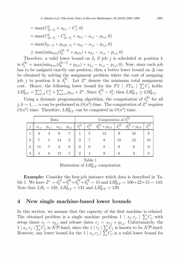
In the computation of LB1WT , it is implicitly assumed that a job is not preceded

by any job. However, this is only valid for the first scheduled job. For anyother job j, the setup operation on M2 has to wait until the predecessor of jobj finishes its processing. Consequently, if a job j is not the first scheduled job,then a better lower bound on δj is δ

2j = max(0, s2,j − s1,j − p1,j +minh �=j(δ

1h +

p2,h)) (see figure 2). Therefore, if a particular job j0 is the first one to beprocessed, then a lower bound on the total waiting time is δ1j0 +

∑j �=j0

δ2j .

Hence, a valid lower bound for the F2 | STsi |∑

Cj is LB2WT =

∑n

j=1C1j +∑n

j=1 p2,j +Δ′, where Δ′ = minj0=1,...,n(δ1j0+∑

j �=j0δ2j ).

The computation of Δ′ requires O(n) time. Thus, LB2WT can be computed

in O(n logn) time. Clearly, we have LB2WT ≥ LB1

WT .

M2

M1s1,j0 p1,j0

s2,j0 p2,j0

δj0

...

...

s1,j p1,j

s2,j p2,j

δ2jmin(δ1h + p2,h)

Fig. 2. Illustration of δ2j computation

3.3 A multiple predecessor-based lower bound

Let Ci,j denote the completion time of job j on machineMi (i = 1, 2). Actually,

we have δj = C2,j − p2,j − C1,j. Let [k] denote the job in position k, and δ[k]j

denote a lower bound on δj if job j is scheduled at position k. Obviously,

δ[1]j = δ1j . Now, if job j is scheduled at position k ≥ 2, then we have C1

j =C1

[k−1] + s1,j + p1,j and C2j = max(C2

[k−1] + s2,j, C1j ) + p2,j. Consequently, we

have:

δj = C2j − p2,j − C1

j

= max(C2[k−1] + s2,j, C

1j )− C1

j

A. Gharbi et al. / Electronic Notes in Discrete Mathematics 36 (2010) 1089–10961092

= max(C2[k−1] + s2,j − C1

j , 0)

= max(C2[k−1] − C1

[k−1] + s2,j − s1,j − p1,j , 0)

= max(δ[k−1] + p2,[k−1] + s2,j − s1,j − p1,j, 0)

≥ max(minh �=j(δ[k−1]h + p2,h) + s2,j − s1,j − p1,j, 0)

Therefore, a valid lower bound on δj if job j is scheduled at position k

is δ[k]j = max(minh �=j(δ

[k−1]h + p2,h) + s2,j − s1,j − p1,j, 0). Now, since each job

has to be assigned exactly one position, then a better lower bound on Δ canbe obtained by solving the assignment problem where the cost of assigningjob j to position k is δ

[k]j . Let Z∗ denote the minimum total assignment

cost. Hence, the following lower bound for the F2 | STsi |∑

Cj holds:

LB3WT =

∑n

j=1C1j +

∑n

j=1 p2,j + Z∗. Since δ[2]j = δ2j , then LB3

WT ≥ LB2WT .

Using a dynamic programming algorithm, the computation of δ[k]j for all

j, k = 1, ..., n can be performed in O(n2) time. The computation of Z∗ requiresO(n3) time. Therefore, LB3

WT can be computed in O(n3) time.

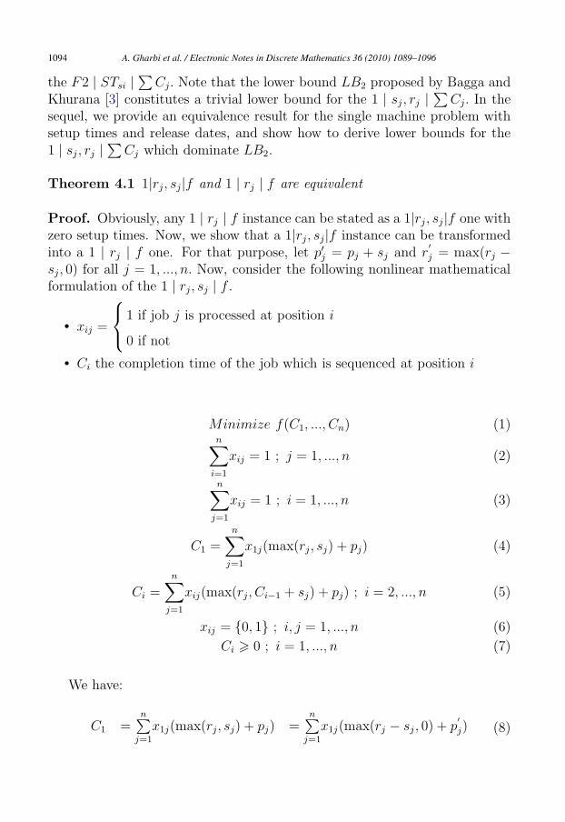
Data Computation of δ[k]j

j s1,j p1,j s2,j p2,j δ[1]j δ

[2]j δ

[2]h + p2,h δ

[3]j δ

[3]h + p2,h δ

[4]j

1 3 4 8 7 1 5 12 9 16 9

2 7 5 14 2 2 7 9 10 12 10

3 11 7 2 8 0 0 8 0 8 0

4 4 8 12 5 0 4 9 8 3 8

Table 1Illustration of LB3

WT computation

Example: Consider the four-job instance which data is described in Ta-ble 1. We have Z∗ = δ

[1]2 +δ

[2]1 +δ

[3]4 +δ

[4]3 = 15 and LB3

WT = 106+22+15 = 143.Note that LB1 = 128, LB1

WT = 131 and LB2WT = 139.

4 New single machine-based lower bounds

In this section, we assume that the capacity of the first machine is relaxed.The obtained problem is a single machine problem 1 | sj , rj |

∑Cj with

setup times sj = s2,j and release dates rj = s1,j + p1,j . Unfortunately, the1 | sj , rj |

∑Cj is NP-hard, since the 1 | rj |

∑Cj is known to be NP-hard.

However, any lower bound for the 1 | sj , rj |∑

Cj is a valid lower bound for

A. Gharbi et al. / Electronic Notes in Discrete Mathematics 36 (2010) 1089–1096 1093

the F2 | STsi |∑

Cj. Note that the lower bound LB2 proposed by Bagga andKhurana [3] constitutes a trivial lower bound for the 1 | sj , rj |

∑Cj. In the

sequel, we provide an equivalence result for the single machine problem withsetup times and release dates, and show how to derive lower bounds for the1 | sj , rj |

∑Cj which dominate LB2.

Theorem 4.1 1|rj, sj|f and 1 | rj | f are equivalent

Proof. Obviously, any 1 | rj | f instance can be stated as a 1|rj, sj |f one withzero setup times. Now, we show that a 1|rj, sj|f instance can be transformedinto a 1 | rj | f one. For that purpose, let p′j = pj + sj and r

′

j = max(rj −sj, 0) for all j = 1, ..., n. Now, consider the following nonlinear mathematicalformulation of the 1 | rj , sj | f .

• xij =

⎧⎨⎩

1 if job j is processed at position i

0 if not

• Ci the completion time of the job which is sequenced at position i

Minimize f(C1, ..., Cn) (1)n∑

i=1

xij = 1 ; j = 1, ..., n (2)

n∑j=1

xij = 1 ; i = 1, ..., n (3)

C1 =n∑

j=1

x1j(max(rj, sj) + pj) (4)

Ci =

n∑j=1

xij(max(rj, Ci−1 + sj) + pj) ; i = 2, ..., n (5)

xij = {0, 1} ; i, j = 1, ..., n (6)

Ci � 0 ; i = 1, ..., n (7)

We have:

C1 =n∑

j=1

x1j(max(rj, sj) + pj) =n∑

j=1

x1j(max(rj − sj , 0) + p′

j) (8)

A. Gharbi et al. / Electronic Notes in Discrete Mathematics 36 (2010) 1089–10961094

Similarly, we have:

Ci =n∑

j=1

xij(max(rj , Ci−1 + sj) + pj) =n∑

j=1

xij(max(rj − sj, Ci−1) + p′

j)

(9)

Since Ci−1 � 0, then we have:

Ci =n∑

j=1

xij(max(0, rj − sj, Ci−1) + p′

j)

=n∑

j=1

xij(max(max(0, rj − sj), Ci−1) + p′

j)(10)

Therefore, if constraints 4 and 5 are replaced by 8 and 10, respectively,then we obtain an equivalent 1|rj|f formulation with processing times p

′

j and

release dates r′

j. �

Corollary 4.2 1|rj, sj |∑

Cj and 1|rj|∑

Cj are equivalent

Consequently, valid lower bounds for the 1 | rj , sj |∑

Cj can be derived byusing the above transformation. A first single machine-based lower bound forF2 | STsi |

∑Cj, denoted hereafter by LB1

SM , can be derived by computingthe optimal total completion time of the preemptive version of the obtained1 | rj |

∑Cj problem. LB1

SM can be computed in O(n logn) by using theSRPT rule.

Interestingly, T’Kindt and Della Croce [4] proposed an improved preemp-tive lower bound for the 1 | rj |

∑Cj which can be computed in O(n logn)

time. Clearly, their result can be used to derive a second single machine-basedlower bound for the F2 | STsi |

∑Cj, denoted herafter by LB2

SM . Obviously,we have LB2

SM ≥ LB1SM .

5 Preliminary computational results

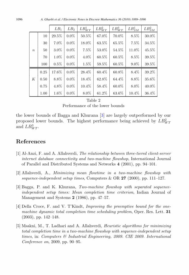
In order to assess the quality of the different proposed lower bounds, we carriedout a series of experiments on randomly generated instances. The processingand setup times were randomly generated from uniform distributions with pi,jfrom [1, 100] and si,j from [0, 100K], where K ∈ {0.25, 0.5, 0.75, 1}. Thenumber of jobs n was taken equal to 10, 30, 50, 70 and 100. Fifty replicateswere generated for each problem size and each value of K.

Table 2 reports, for each lower bound, the percentage of times it yields themaximal value over all of the bounds described in this paper. It is clear that

A. Gharbi et al. / Electronic Notes in Discrete Mathematics 36 (2010) 1089–1096 1095

LB1 LB2 LB1WT LB2

WT LB3WT LB1

SM LB2SM

10 29.5% 0.0% 50.5% 67.0% 70.0% 8.5% 30.0%

30 7.0% 0.0% 18.0% 63.5% 65.5% 7.5% 34.5%

n 50 3.0% 0.0% 7.5% 53.0% 54.5% 11.0% 45.5%

70 1.0% 0.0% 4.0% 60.5% 60.5% 8.5% 39.5%

100 0.5% 0.0% 1.5% 59.5% 60.5% 9.0% 39.5%

0.25 17.6% 0.0% 28.4% 60.4% 60.8% 8.4% 39.2%

K 0.50 8.8% 0.0% 18.4% 62.8% 64.4% 8.8% 35.6%

0.75 4.8% 0.0% 10.4% 58.4% 60.0% 8.0% 40.0%

1.00 1.6% 0.0% 8.0% 61.2% 63.6% 10.4% 36.4%

Table 2Performance of the lower bounds

the lower bounds of Bagga and Khurana [3] are largely outperformed by ourproposed lower bounds. The highest performance being achieved by LB2

WT

and LB3WT .

References

[1] Al-Anzi, F. and A. Allahverdi, The relationship between three-tiered client-server

internet database connectivity and two-machine flowshop, International Journalof Parallel and Distributed Systems and Networks 4 (2001), pp. 94–101.

[2] Allahverdi, A., Minimizing mean flowtime in a two-machine flowshop with

sequence-independent setup times, Computers & OR 27 (2000), pp. 111–127.

[3] Bagga, P. and K. Khurana, Two-machine flowshop with separated sequence-

independent setup times: Mean completion time criterion, Indian Journal ofManagement and Systems 2 (1986), pp. 47–57.

[4] Della Croce, F. and V. T’Kindt, Improving the preemptive bound for the one-

machine dynamic total completion time scheduling problem, Oper. Res. Lett. 31(2003), pp. 142–148.

[5] Msakni, M., T. Ladhari and A. Allahverdi, Heuristic algorithms for minimizing

total completion time in a two-machine flowshop with sequence-independent setup

times, in: Computers & Industrial Engineering, 2009. CIE 2009. International

Conference on, 2009, pp. 90–95.

A. Gharbi et al. / Electronic Notes in Discrete Mathematics 36 (2010) 1089–10961096