Embed Size (px)
Citation preview
Positioning and Navigation Using the Russian Satellite SystemGLONASS
von
Udo Roßbach
Vollstandiger Abdruck der von der Fakultat fur Bauingenieur- und Vermessungswesen der Universitatder Bundeswehr Munchen zur Erlangung des akademischen Grades eines Doktor-Ingenieurs (Dr.-Ing.)genehmigten Dissertation.
Vorsitzender: Univ.-Prof. Dr.-Ing. W. Reinhardt
1. Berichterstatter: Univ.-Prof. Dr.-Ing. G. W. Hein
2. Berichterstatter: Univ.-Prof. Dr.-Ing. E. Groten
3. Berichterstatter: Univ.-Prof. Dr.-Ing. B. Eissfeller
Die Dissertation wurde am 2. Marz 2000 bei der Universitat der Bundeswehr Munchen, Werner-Heisen-berg-Weg 39, D-85577 Neubiberg eingereicht.
Tag der mundlichen Prufung: 20. Juni 2000
ii ABSTRACT / ZUSAMMENFASSUNG
Abstract
Satellite navigation systems have not only revolutionized navigation, but also geodetic positioning. Bymeans of satellite range measurements, positioning accuracies became available that were previouslyunknown, especially for long baselines. This has long been documented for applications of GPS, theAmerican Global Positioning System. Besides this, there is the Russian Global Navigation Satellite Sys-tem GLONASS. Comparable to GPS from the technical point of view, it is suffering under the economicdecline of the Russian Federation, which prevents it from drawing the attention it deserves.
Due to the similarities of GPS and GLONASS, both systems may also be used in combined ap-plications. However, since both systems are not entirely compatible to each other, first a number ofinter-operability issues have to be solved. Besides receiver hardware issues, these are mainly the differ-ences in coordinate and time reference frames. For both issues, proposed solutions are provided. Forthe elimination of differences in coordinate reference frames, possible coordinate transformations areintroduced, determined using both a conventional and an innovative approach.
Another important topic in the usage of GLONASS for high-precision applications is the fact thatGLONASS satellites are distinguished by slightly different carrier frequencies instead of different PRNcodes. This results in complications, when applying double difference carrier phase measurements toposition determination the way it is often done with GPS. To overcome these difficulties and make useof GLONASS double difference carrier phase measurements for positioning, a new mathematical modelfor double difference carrier phase observations has been developed.
These solutions have been implemented in a GLONASS and combined GPS/GLONASS processingsoftware package.
Zusammenfassung
Satelliten-Navigationssysteme haben nicht nur die Navigation, sondern auch die geodatische Positionsbe-stimmung revolutioniert. Mit Hilfe von Entfernungsmessungen zu Satelliten wurden vorher nicht gekannteGenauigkeiten in der Positionierung verfugbar. Fur Anwendungen des amerikanischen GPS Global Po-sitioning System ist dies schon lange dokumentiert. Daneben gibt es das russische Global NavigationSatellite System GLONASS. Vom technischen Standpunkt her vergleichbar zu GPS, leidet es unter demwirtschaftlichen Niedergang der Russischen Foderation und erhalt deswegen nicht die Aufmerksamkeit,die es verdient.
Aufgrund der Ahnlichkeiten zwischen GPS und GLONASS konnen beide System auch gemeinsamin kombinierten Anwendungen genutzt werden. Da beide System jedoch nicht vollstandig zueinanderkompatibel sind, mussen vorher noch einige Fragen der gemeinsamen Nutzung geklart werden. NebenFragen der Empfanger-Hardware sind dies hauptsachlich die Unterschiede in den Koordinaten- undZeit-Bezugssystemen. Fur beide Punkte wurden Losungen vorgeschlagen. Um die Unterschiede in denKoordinaten-Bezugssystemen auszuraumen, werden mogliche Koordinatentransformationen vorgestellt.Diese wurden sowohl uber einen konventionellen als auch mit einem innovativen Ansatz bestimmt.
Ein anderer wichtiger Punkt in der Nutzung von GLONASS fur hochprazise Anwendungen ist dieTatsache, daß sich GLONASS-Satelliten durch die leicht unterschiedlichen Tragerfrequenzen ihrer Sig-nale unterscheiden, und nicht durch unterschiedliche PRN-Codes. Dies bringt Komplikationen mitsich bei der Anwendung doppelt-differenzierter Tragerphasenmessungen, wie sie bei GPS haufig ver-wendet werden. Um diese Schwierigkeiten zu uberwinden und auch doppelt differenzierte GLONASS-Tragerphasenmessungen fur die Positionsbestimmung verwenden zu konnen, wurde ein neues mathema-tisches Modell der Doppeldifferenz-Phasenbeobachtungen hergeleitet.
Die gewonnenen Erkenntnisse wurden in einem Software-Paket zur Prozessierung von GLONASS undkombinierten GPS/GLONASS Beobachtungen implementiert.
CONTENTS iii
Contents
Abstract / Zusammenfassung ii
Contents iii
List of Figures vi
List of Tables viii
1 Introduction 1
2 History of the GLONASS System 3
3 GLONASS System Description 73.1 Reference Systems . . . . . . . . . . . . . . . . . . . . . . . . . . . . . . . . . . . . . . . . 7
3.1.1 Time Systems . . . . . . . . . . . . . . . . . . . . . . . . . . . . . . . . . . . . . . . 73.1.2 Coordinate Systems . . . . . . . . . . . . . . . . . . . . . . . . . . . . . . . . . . . 7
3.2 Ground Segment . . . . . . . . . . . . . . . . . . . . . . . . . . . . . . . . . . . . . . . . . 83.3 Space Segment . . . . . . . . . . . . . . . . . . . . . . . . . . . . . . . . . . . . . . . . . . 93.4 GLONASS Frequency Plan . . . . . . . . . . . . . . . . . . . . . . . . . . . . . . . . . . . 103.5 Signal Structure . . . . . . . . . . . . . . . . . . . . . . . . . . . . . . . . . . . . . . . . . 12
3.5.1 C/A-Code . . . . . . . . . . . . . . . . . . . . . . . . . . . . . . . . . . . . . . . . . 123.5.2 P-Code . . . . . . . . . . . . . . . . . . . . . . . . . . . . . . . . . . . . . . . . . . 143.5.3 C/A-Code Data Sequence . . . . . . . . . . . . . . . . . . . . . . . . . . . . . . . . 143.5.4 Time Code . . . . . . . . . . . . . . . . . . . . . . . . . . . . . . . . . . . . . . . . 143.5.5 Bit Synchronization . . . . . . . . . . . . . . . . . . . . . . . . . . . . . . . . . . . 153.5.6 Structure of Navigation Data . . . . . . . . . . . . . . . . . . . . . . . . . . . . . . 153.5.7 GLONASS-M Navigation Data . . . . . . . . . . . . . . . . . . . . . . . . . . . . . 16
3.6 System Assurance Techniques . . . . . . . . . . . . . . . . . . . . . . . . . . . . . . . . . . 193.7 User Segment and Receiver Development . . . . . . . . . . . . . . . . . . . . . . . . . . . 243.8 GLONASS Performance . . . . . . . . . . . . . . . . . . . . . . . . . . . . . . . . . . . . . 29
4 Time Systems 314.1 GLONASS Time . . . . . . . . . . . . . . . . . . . . . . . . . . . . . . . . . . . . . . . . . 314.2 GPS Time . . . . . . . . . . . . . . . . . . . . . . . . . . . . . . . . . . . . . . . . . . . . . 314.3 UTC, UTCUSNO, UTCSU and GLONASS System Time . . . . . . . . . . . . . . . . . . 324.4 Resolving the Time Reference Difference . . . . . . . . . . . . . . . . . . . . . . . . . . . . 33
4.4.1 Introducing a Second Receiver Clock Offset . . . . . . . . . . . . . . . . . . . . . . 334.4.2 Introducing the Difference in System Time Scales . . . . . . . . . . . . . . . . . . . 344.4.3 Application of A-priori Known Time Offsets . . . . . . . . . . . . . . . . . . . . . . 354.4.4 Dissemination of Difference in Time Reference . . . . . . . . . . . . . . . . . . . . 36
4.5 Conclusions . . . . . . . . . . . . . . . . . . . . . . . . . . . . . . . . . . . . . . . . . . . . 36
5 Coordinate Systems 395.1 PZ-90 (GLONASS) . . . . . . . . . . . . . . . . . . . . . . . . . . . . . . . . . . . . . . . . 395.2 WGS84 (GPS) . . . . . . . . . . . . . . . . . . . . . . . . . . . . . . . . . . . . . . . . . . 395.3 Realizations . . . . . . . . . . . . . . . . . . . . . . . . . . . . . . . . . . . . . . . . . . . . 405.4 Combining Coordinate Frames . . . . . . . . . . . . . . . . . . . . . . . . . . . . . . . . . 405.5 7-Parameter Coordinate Transformation . . . . . . . . . . . . . . . . . . . . . . . . . . . . 425.6 Transformation Parameters . . . . . . . . . . . . . . . . . . . . . . . . . . . . . . . . . . . 42
5.6.1 Methods for Determination of Transformation Parameters . . . . . . . . . . . . . . 42
iv CONTENTS
5.6.2 Russian Estimations . . . . . . . . . . . . . . . . . . . . . . . . . . . . . . . . . . . 435.6.3 American Estimations . . . . . . . . . . . . . . . . . . . . . . . . . . . . . . . . . . 445.6.4 German Estimations . . . . . . . . . . . . . . . . . . . . . . . . . . . . . . . . . . . 445.6.5 IGEX-98 Estimations . . . . . . . . . . . . . . . . . . . . . . . . . . . . . . . . . . 45
5.7 Applying the Coordinate Transformation . . . . . . . . . . . . . . . . . . . . . . . . . . . 465.8 Coordinate Frames in Differential Processing . . . . . . . . . . . . . . . . . . . . . . . . . 505.9 GLONASS Ephemerides in WGS84 . . . . . . . . . . . . . . . . . . . . . . . . . . . . . . . 53
6 Determination of Transformation Parameters 556.1 Preparations and Realization of IfEN’s Measurement Campaign . . . . . . . . . . . . . . . 556.2 Data Analysis . . . . . . . . . . . . . . . . . . . . . . . . . . . . . . . . . . . . . . . . . . . 57
6.2.1 Single Point Positioning . . . . . . . . . . . . . . . . . . . . . . . . . . . . . . . . . 586.2.2 Double Difference Baselines . . . . . . . . . . . . . . . . . . . . . . . . . . . . . . . 61
6.3 Direct Estimation of Transformation Parameters . . . . . . . . . . . . . . . . . . . . . . . 62
7 Satellite Clock and Orbit Determination 737.1 Satellite Clock Offset . . . . . . . . . . . . . . . . . . . . . . . . . . . . . . . . . . . . . . . 737.2 Satellite Orbit Determination . . . . . . . . . . . . . . . . . . . . . . . . . . . . . . . . . . 74
7.2.1 Orbital Force Model . . . . . . . . . . . . . . . . . . . . . . . . . . . . . . . . . . . 747.2.2 Orbit Integration . . . . . . . . . . . . . . . . . . . . . . . . . . . . . . . . . . . . . 777.2.3 Integration Error . . . . . . . . . . . . . . . . . . . . . . . . . . . . . . . . . . . . . 78
7.3 Satellite Positions from Almanac Data . . . . . . . . . . . . . . . . . . . . . . . . . . . . . 83
8 Observations and Position Determination 858.1 Pseudorange Measurements . . . . . . . . . . . . . . . . . . . . . . . . . . . . . . . . . . . 85
8.1.1 Single Point Positioning . . . . . . . . . . . . . . . . . . . . . . . . . . . . . . . . . 858.1.2 Single Difference Positioning . . . . . . . . . . . . . . . . . . . . . . . . . . . . . . 918.1.3 Double Difference Positioning . . . . . . . . . . . . . . . . . . . . . . . . . . . . . . 96
8.2 Carrier Phase Measurements . . . . . . . . . . . . . . . . . . . . . . . . . . . . . . . . . . 1038.2.1 Single Point Observation Equation . . . . . . . . . . . . . . . . . . . . . . . . . . . 1038.2.2 Single Difference Positioning . . . . . . . . . . . . . . . . . . . . . . . . . . . . . . 1058.2.3 Double Difference Positioning . . . . . . . . . . . . . . . . . . . . . . . . . . . . . . 106
8.3 GLONASS and GPS/GLONASS Carrier Phase Positioning . . . . . . . . . . . . . . . . . 1118.3.1 Floating GLONASS Ambiguities . . . . . . . . . . . . . . . . . . . . . . . . . . . . 1118.3.2 Single Difference Positioning and Receiver Calibration . . . . . . . . . . . . . . . . 1118.3.3 Scaling to a Common Frequency . . . . . . . . . . . . . . . . . . . . . . . . . . . . 1128.3.4 Iterative Ambiguity Resolution . . . . . . . . . . . . . . . . . . . . . . . . . . . . . 113
8.4 A Proposed Solution to the Frequency Problem . . . . . . . . . . . . . . . . . . . . . . . . 1148.5 Ionospheric Correction . . . . . . . . . . . . . . . . . . . . . . . . . . . . . . . . . . . . . . 120
8.5.1 Single Frequency Ionospheric Correction . . . . . . . . . . . . . . . . . . . . . . . . 1208.5.2 Dual Frequency Ionospheric Correction . . . . . . . . . . . . . . . . . . . . . . . . 123
8.6 Dilution of Precision . . . . . . . . . . . . . . . . . . . . . . . . . . . . . . . . . . . . . . . 126
9 GPS/GLONASS Software Tools 135
10 Summary 139
Appendix 141
A Bibliography 141
B GLONASS Launch History 149
CONTENTS v
C Symbols 151C.1 Symbols Used in Mathematical Formulae . . . . . . . . . . . . . . . . . . . . . . . . . . . 151C.2 Vectors and Matrices . . . . . . . . . . . . . . . . . . . . . . . . . . . . . . . . . . . . . . . 151C.3 Symbols Used as Subscripts . . . . . . . . . . . . . . . . . . . . . . . . . . . . . . . . . . . 152C.4 Symbols Used as Superscripts . . . . . . . . . . . . . . . . . . . . . . . . . . . . . . . . . . 152
D Abbreviations and Acronyms 153
Dank 157
Lebenslauf 159
vi LIST OF FIGURES
List of Figures
2.1 Number of available satellites in 1996 through 1999 . . . . . . . . . . . . . . . . . . . . . . 52.2 Current status of the GLONASS space segment . . . . . . . . . . . . . . . . . . . . . . . . 53.1 Locations of GLONASS ground stations . . . . . . . . . . . . . . . . . . . . . . . . . . . . 93.2 Model of GLONASS satellite . . . . . . . . . . . . . . . . . . . . . . . . . . . . . . . . . . 113.3 GLONASS frequency plan . . . . . . . . . . . . . . . . . . . . . . . . . . . . . . . . . . . . 133.4 GLONASS C/A-code generation . . . . . . . . . . . . . . . . . . . . . . . . . . . . . . . . 133.5 GLONASS P-code generation . . . . . . . . . . . . . . . . . . . . . . . . . . . . . . . . . . 143.6 Structure of the C/A-code data sequence . . . . . . . . . . . . . . . . . . . . . . . . . . . 153.7 Structure of ephemeris and general data lines . . . . . . . . . . . . . . . . . . . . . . . . . 173.8 Structure of almanac data lines . . . . . . . . . . . . . . . . . . . . . . . . . . . . . . . . . 173.9 Structure of ephemeris and general data lines (GLONASS-M) . . . . . . . . . . . . . . . . 203.10 Structure of almanac data lines (GLONASS-M) . . . . . . . . . . . . . . . . . . . . . . . . 213.11 Single point positioning using GPS . . . . . . . . . . . . . . . . . . . . . . . . . . . . . . . 223.12 Single point positioning using GLONASS . . . . . . . . . . . . . . . . . . . . . . . . . . . 233.13 3S Navigation R-100/R-101 GPS/GLONASS receiver . . . . . . . . . . . . . . . . . . . . 253.14 MAN / 3S Navigation GNSS-200 GPS/GLONASS receiver . . . . . . . . . . . . . . . . . 263.15 Ashtech GG24 GPS/GLONASS receiver OEM board . . . . . . . . . . . . . . . . . . . . . 273.16 Javad Positioning Systems GPS/GLONASS receivers . . . . . . . . . . . . . . . . . . . . . 283.17 NovAtel MiLLenium–GLONASS GPS/GLONASS receiver OEM board . . . . . . . . . . 285.1 Example of combined GPS/GLONASS positioning without coordinate transformation . . 415.2 Example of combined GPS/GLONASS positioning with coordinate transformation accord-
ing to (Misra et al., 1996a) . . . . . . . . . . . . . . . . . . . . . . . . . . . . . . . . . . . 475.3 Example of combined GPS/GLONASS positioning with coordinate transformation accord-
ing to (Roßbach et al., 1996) . . . . . . . . . . . . . . . . . . . . . . . . . . . . . . . . . . 485.4 Example of combined GPS/GLONASS positioning with coordinate transformation accord-
ing to (Mitrikas et al., 1998) . . . . . . . . . . . . . . . . . . . . . . . . . . . . . . . . . . 495.5 Average deviations of differential positions with and without transformation . . . . . . . . 525.6 Deviations of differential kinematic positions with and without transformation . . . . . . 536.1 Participating observation sites . . . . . . . . . . . . . . . . . . . . . . . . . . . . . . . . . . 566.2 Observation sites used for direct estimation of transformation parameters . . . . . . . . . 707.1 Determination of integration error in satellite orbit calculation . . . . . . . . . . . . . . . 797.2 Example of orbit errors in dependence of step width . . . . . . . . . . . . . . . . . . . . . 807.3 Determination of long term integration error . . . . . . . . . . . . . . . . . . . . . . . . . 817.4 Long-term errors in orbit integration . . . . . . . . . . . . . . . . . . . . . . . . . . . . . . 828.1 GPS, GLONASS and combined GPS/GLONASS absolute positioning . . . . . . . . . . . 908.2 GPS, GLONASS and GPS/GLONASS absolute positioning, height component . . . . . . 918.3 GPS, GLONASS and combined GPS/GLONASS single difference positioning . . . . . . . 958.4 GPS, GLONASS and GPS/GLONASS single difference positioning, height component . . 968.5 GPS, GLONASS and combined GPS/GLONASS double difference positioning . . . . . . 1018.6 GPS, GLONASS and GPS/GLONASS double difference positioning, height component . 1028.7 GPS/GLONASS double difference inter-system hardware delay . . . . . . . . . . . . . . . 1038.8 GPS, GLONASS and GPS/GLONASS single difference carrier phase positioning . . . . . 1078.9 Single difference carrier phase positioning, position deviation . . . . . . . . . . . . . . . . 1088.10 GPS, GLONASS and GPS/GLONASS double difference carrier phase positioning . . . . . 1198.11 Double difference carrier phase positioning, position deviation . . . . . . . . . . . . . . . . 1208.12 GPS/GLONASS double difference carrier phase inter-system hardware delay . . . . . . . 1218.13 GPS double difference carrier phase floating ambiguities . . . . . . . . . . . . . . . . . . . 1228.14 GLONASS double difference carrier phase floating ambiguities . . . . . . . . . . . . . . . 122
LIST OF FIGURES vii
8.15 GDOP values for 02/26/99 . . . . . . . . . . . . . . . . . . . . . . . . . . . . . . . . . . . 1318.16 Comparison of GDOP values from Eqs. (8.6.12) and (8.6.15) . . . . . . . . . . . . . . . . 1328.17 Comparison of PDOP values from Eqs. (8.6.12) and (8.6.15) . . . . . . . . . . . . . . . . 1338.18 Comparison of TDOP values from Eqs. (8.6.12) and (8.6.15) . . . . . . . . . . . . . . . . 1339.1 Screen shot of the GPS/GLONASS mission planning tool . . . . . . . . . . . . . . . . . . 1379.2 Screen shot of the GPS/GLONASS RINEX decoder . . . . . . . . . . . . . . . . . . . . . 1379.3 Screen shot of the GPS/GLONASS absolute positioning tool . . . . . . . . . . . . . . . . 138
viii LIST OF TABLES
List of Tables
3.1 Parameters of the reference systems PZ-90 and WGS84 . . . . . . . . . . . . . . . . . . . 83.2 Mean square errors of GLONASS broadcast ephemerides . . . . . . . . . . . . . . . . . . . 93.3 Parameters of the GLONASS and GPS space segments . . . . . . . . . . . . . . . . . . . . 103.4 Usage of GLONASS frequency numbers in January of 1998 . . . . . . . . . . . . . . . . . 123.5 Structure of lines 1 – 5 . . . . . . . . . . . . . . . . . . . . . . . . . . . . . . . . . . . . . . 163.6 Structure of lines 6 – 15 . . . . . . . . . . . . . . . . . . . . . . . . . . . . . . . . . . . . . 183.7 New or modified GLONASS-M data fields in lines 1 – 5 . . . . . . . . . . . . . . . . . . . 193.8 Accuracy of measurements indicator FT . . . . . . . . . . . . . . . . . . . . . . . . . . . . 193.9 New or modified GLONASS-M data fields in lines 6 – 15 . . . . . . . . . . . . . . . . . . . 206.1 Known station coordinates in ITRF-94 . . . . . . . . . . . . . . . . . . . . . . . . . . . . . 566.2 Summary of available observations at stations by campaign day . . . . . . . . . . . . . . . 576.3 Computed station coordinates in the PZ-90 frame . . . . . . . . . . . . . . . . . . . . . . . 586.4 Estimated transformation parameters from single point solutions, 7 parameters . . . . . . 596.5 Residuals of 7 parameter transformation . . . . . . . . . . . . . . . . . . . . . . . . . . . . 606.6 Estimated transformation parameters from single point solutions, 4 parameters . . . . . . 606.7 Known baselines between stations in ITRF-94 . . . . . . . . . . . . . . . . . . . . . . . . . 616.8 Computed baselines between stations . . . . . . . . . . . . . . . . . . . . . . . . . . . . . . 616.9 Estimated transformation parameters from baseline solutions, 4 parameters . . . . . . . . 626.10 Coordinates of observation sites used in parameter determination . . . . . . . . . . . . . . 717.1 Errors in orbit integration of center epoch between two adjacent ephemerides . . . . . . . 797.2 Errors in orbit integration to reference epoch of succeeding ephemerides . . . . . . . . . . 797.3 Errors in orbit integration to reference epoch of preceding ephemerides . . . . . . . . . . . 807.4 Long-term errors in orbit integration . . . . . . . . . . . . . . . . . . . . . . . . . . . . . . 828.1 Largest common denominators of GLONASS/GLONASS coefficients, until 2005 . . . . . . 1178.2 Largest common denominators of GLONASS/GLONASS coefficients, beyond 2005 . . . . 118B.1 Launch history and service lives of GLONASS satellites . . . . . . . . . . . . . . . . . . . 149
1
1 Introduction
Parallel to the American NAVSTAR-GPS, the former Soviet Union also worked on developing and puttingup a satellite navigation system based on one-way range measurements. This system, called GLONASS(GLONASS – Global~na� Navigacionna� Sputnikova� Sistema, Global’naya NavigatsionnayaSputnikowaya Sistema, Global Navigation Satellite System), today is continued by the Commonwealthof Independent States (CIS) and especially the Russian Federation as the successor of the Soviet Union.
Like its American counter-piece, GLONASS is intended to provide an unlimited number of users atany time on any place on Earth in any weather with highly precise position and velocity fixes. Theprinciple of GLONASS is equivalent to that of its American counter-piece. Each satellite carries anatomic clock and transmits radio signals, which contain clock readings as well as information on thesatellite orbit and the satellite clock offset from system time. The user receives these satellite signals andcompares the time of signal transmission with the time of signal reception, as read on the receiver’s ownclock. The difference of these two clock readings, multiplied by the speed of light, equals the distancebetween the satellite and the user. Four such one-way distance measurements to four different satellitessimultaneously, together with the satellite position and clock offsets known from the orbit data, yieldthe three coordinates of the user’s position and the user’s clock offset with respect to system time as thefourth unknown.
Equivalent to the Standard Positioning Service (SPS) and the Precise Positioning Service (PPS)of GPS, GLONASS provides a standard precision (SP) navigation signal and a high precision (HP)navigation signal. These signals are sometimes also referred to as Channel of Standard Accuracy (CSA)and Channel of High Accuracy (CHA), respectively. The SP signal is available to all civil users world-wideon a continuous basis. Accuracy of GLONASS navigation using the SP signal is specified to be 50 - 70 m(99.7 %) in the horizontal plane and 70 m (99.7 %) in height. Accuracy of estimated velocity vectors is15 cm/s (99.7 %). Timing accuracy is 1 µs (99.7 %) (CSIC, 1998). These accuracies can be increasedusing dual-frequency P-code measurements of the HP signal. A further increase is possible in differentialoperation.
Applications of GLONASS are equivalent to those of GPS and can be seen mostly in highly precisenavigation of land, sea, air and low orbiting spacecraft (CSIC, 1994). Besides this, GLONASS is alsosuitable for the dissemination of highly precise global and local time scales as well as for establishing globalgeodetic coordinate systems and local geodetic networks. The system can also be used for providingprecise coordinates for cadastre works. Further usage could contain the support of research work ingeology, geophysics, geodynamics, oceanography and others by providing position and time information.Similar uses are possible for large scale construction projects.
With this range of applications and the achievable accuracy, GLONASS has become an attractivetool for navigational and geodetic purposes. But not only GLONASS as a stand-alone system drawsthe interest of scientists around the world. The fact that there are two independent, but generally verysimilar satellite navigation systems also draws attention to the combined use of both systems. Thiscombined use brings up a number of advantages. At first, the number of available (observable) satellitesis increased with respect to one single system. This will provide a user with a better satellite geometryand more redundant information, allowing him to compute a more accurate position fix. In cases withobstructed visibility of the sky, such as mountainous or urban areas, a position fix might not be possibleat all without these additional satellites. Besides that, the more satellite measurements are available,the earlier and more reliably a user can detect and isolate measurement outliers or even malfunctioningsatellites. Thus, the combined use of GPS and GLONASS may aid in Receiver Autonomous IntegrityMonitoring (RAIM), providing better integrity of the position fix than a single system alone (Hein et al.,1997).
In a similar way, an increased number of observed satellites improves and accelerates the determinationof integer ambiguities in high-precision (surveying) applications. Therefore, the combination of GPS and
2 1 INTRODUCTION
GLONASS is expected to provide better performance in RTK surveying than GPS (or GLONASS) alone(Landau and Vollath, 1996).
This doctoral thesis deals with the use of GLONASS for positioning determination in geodesy andnavigation, especially in combination with GPS. To do so, after a brief history of the GLONASS sys-tem in Chapter 2, the system is explained in detail in Chapter 3. The differences to GPS in terms oftime frame (Chapter 4) and coordinate frame (Chapter 5) are worked out and ways are shown, howthese differences can be overcome in combined GPS/GLONASS applications. Chapter 6 provides detailson a measurement campaign carried out by IfEN in cooperation with other institutions to determinea transformation between the GLONASS and GPS coordinate reference frames and presents results ofthis transformation. The algorithms used for GLONASS satellite position and clock offset determina-tion – cornerstones in GLONASS positioning – are described and analyzed in Chapter 7. Afterwards,the different formulations of the GLONASS and combined GPS/GLONASS observation equations areintroduced and assessed in Chapter 8. The implications on GLONASS carrier phase processing causedby the different signal frequencies are identified and possible solutions are shown, as well as the effects ofcombined GPS/GLONASS observations on the DOP values. Finally, in Chapter 9 an overview is givenon different GPS/GLONASS software tools created in connection with this work and used to computethe results presented in this thesis.
3
2 History of the GLONASS System
Development of the GLONASS system started in the mid-1970s, parallel to the American GPS (Bartenevet al., 1994). The first GLONASS satellite was put into orbit October 12, 1982 (CSIC, 1998). By theend of 1985, ten satellites were operational. This marked the end of the so-called pre-operational phase.In the operational phase, beginning 1986, the planned constellation was successively completed. Theseefforts faced a setback in May 1989, when satellite launches were halted for one year because of recentsatellite failures.
The Soviet air and naval forces were considered to be the primary users of GLONASS. But as withGPS, though a military system, the possibilities of civil usage soon were recognized, at first in the areas ofgeodesy and geodynamics. Since May 1987, GLONASS was used for the determination of Earth RotationParameters (ERP). One year later, in May 1988, at the ICAO conference on Future Air NavigationSystems (FANS) in Montreal/Canada, the system was presented to the civil public (Anodina, 1988). Thesystem was offered to be used by the civil aviation community. In the same year, a similar presentationand offer was made at a conference of the IMO.
In 1989/1990, interest in GLONASS grew steadily in the United States and other Western countries.Although at that time only around ten satellites were operational, the capabilities of GLONASS andespecially of the GPS/GLONASS combination were beginning to be seen. In part this may have beenspurred by the US DoD activating Selective Availability on GPS in March 1990 (N.N., 1990a). Exceptfor a brief time during the Gulf War (to allow US and Allied troops to use ”civilian” GPS receivers tocompensate for military P-code receivers not yet being available in sufficient numbers), S/A then was leftactive, leaving the GPS signal intentionally degraded. During that time some initial work on assessingthe value of GLONASS for civil air navigation were started. FAA awarded a contract to Honeywell andNorthwest Airlines to evaluate GLONASS performance on-board a commercial airliner (N.N., 1990d;Hartmann, 1992). This project was mainly aimed at collecting data for the purpose of certificationof future GPS/GLONASS navigation equipment. The Massachusetts Institute of Technology, LincolnLaboratories, started tracking GLONASS satellites and evaluating system performance, availability andintegrity, also on behalf of the FAA (N.N., 1990c; N.N., 1990b).
Also in Europe, interest in GLONASS and combined use of GPS and GLONASS emerged. Especiallyhere, scientists and officials felt uncomfortable with the current state of GPS and GLONASS both beingsystems controlled by one foreign country’s military forces. So tendencies to use GPS and GLONASS asthe basis for a future Civil Navigation Satellite System or a Global Navigation Satellite System (GNSS)under civil control rose strongly in the early 1990s (N.N., 1993a; N.N., 1993b). But before being able toplan for and design such a system, one had to get to know the existing systems very well.
The collapse of the Soviet Union and its successor, the Russian Federation, at first affected the effortsto complete the system. But Russian officials clung to the system. After all, GLONASS was also intendedto replace ground based navigation systems, which are expensive in the vastness of the Russian territory.GLONASS thus was officially commissioned and placed under the auspices of the Russian Military SpaceForces (Voenno Kosmicheski Sily, VKS) September 24, 1993, with 16 satellites operational. In the monthsto follow, however, some of the older spacecraft had to be withdrawn, bringing the number of operationalsatellites down to ten in August 1994. At that point, GLONASS was granted highest priority, whenPresident Yeltsin issued a decree, ordering to have the system completed by the end of 1995 (GPNN,1994). When launched from Baikonur/Kazakhstan, the Proton launch vehicle can simultaneously carrythree GLONASS satellites into orbit. Thus, five more launches were necessary at that time.
On March 7, 1995, the Russian government issued a decree, ordering the Ministry of Defense, theMinistry of Transportation, the Russian Space Agency and the State Committee on the Defense-orientedIndustry to cooperate in completing and further developing GLONASS (including differential referencestations and user equipment) and fostering its civil use (Government, 1995).
To underline this commitment to civil use of GLONASS, the Russian Space Forces had set up aGLONASS Coordinational Scientific Information Center (CSIC) already in early 1995. This is a literal
4 2 HISTORY OF THE GLONASS SYSTEM
but rather bulky translation of the original Russian name Koordinatsionnyj Nauchno-InformatsionnyjTsentr (KNITs) – Koordinacionny$i Nauqno-Informacionny$i Centr (KNIC). The more eleganttranslation ”Coordination Center of Scientific Information (CCSI)” is hardly used. The mission of theCSIC is to continuously provide the civil community with accurate information on the status of thesystem.
The last of the five remaining launches (as of August 1994) took place in December 1995, and onJanuary 18, 1996, the 24th satellite was put into operation. Appendix B shows the launch history ofGLONASS satellites, depicting these continuing advances in the construction of the system.
In February 1996, the Russian Ministry of Transport offered to use the GLONASS SP signal for civilaviation for a period of at least 15 years without direct user fees. At an ICAO meeting in March, thisoffer was discussed. An enhanced Russian offer was presented in July and finally accepted on July 29,1996, by the ICAO (ICAO, 1996).
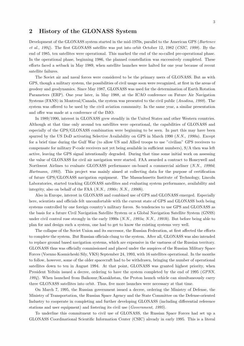
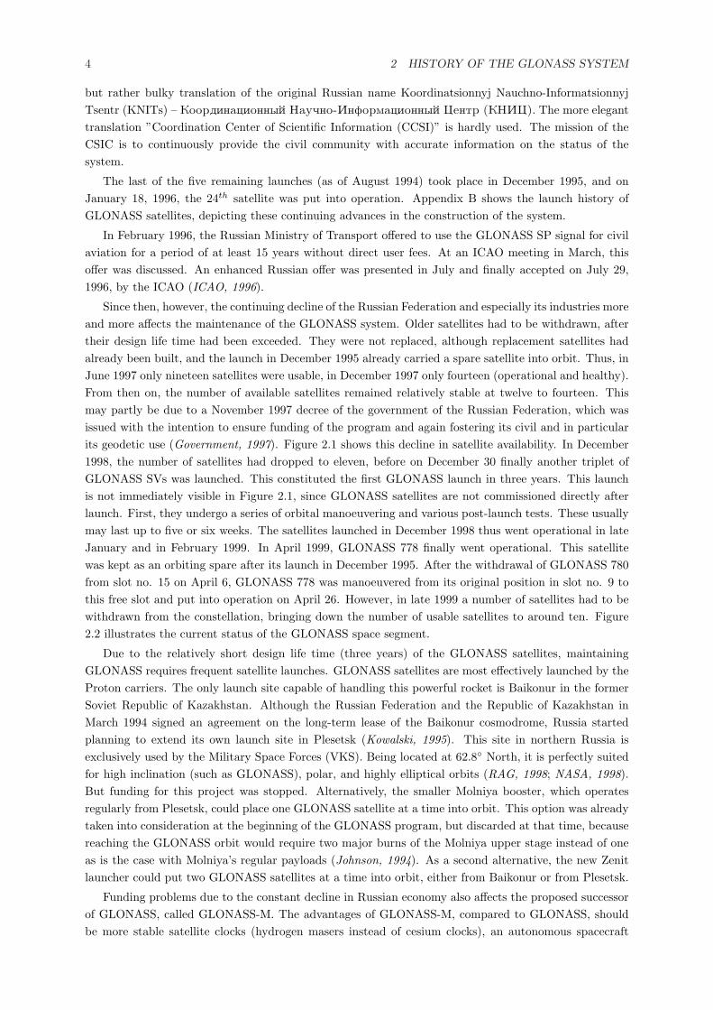
Since then, however, the continuing decline of the Russian Federation and especially its industries moreand more affects the maintenance of the GLONASS system. Older satellites had to be withdrawn, aftertheir design life time had been exceeded. They were not replaced, although replacement satellites hadalready been built, and the launch in December 1995 already carried a spare satellite into orbit. Thus, inJune 1997 only nineteen satellites were usable, in December 1997 only fourteen (operational and healthy).From then on, the number of available satellites remained relatively stable at twelve to fourteen. Thismay partly be due to a November 1997 decree of the government of the Russian Federation, which wasissued with the intention to ensure funding of the program and again fostering its civil and in particularits geodetic use (Government, 1997). Figure 2.1 shows this decline in satellite availability. In December1998, the number of satellites had dropped to eleven, before on December 30 finally another triplet ofGLONASS SVs was launched. This constituted the first GLONASS launch in three years. This launchis not immediately visible in Figure 2.1, since GLONASS satellites are not commissioned directly afterlaunch. First, they undergo a series of orbital manoeuvering and various post-launch tests. These usuallymay last up to five or six weeks. The satellites launched in December 1998 thus went operational in lateJanuary and in February 1999. In April 1999, GLONASS 778 finally went operational. This satellitewas kept as an orbiting spare after its launch in December 1995. After the withdrawal of GLONASS 780from slot no. 15 on April 6, GLONASS 778 was manoeuvered from its original position in slot no. 9 tothis free slot and put into operation on April 26. However, in late 1999 a number of satellites had to bewithdrawn from the constellation, bringing down the number of usable satellites to around ten. Figure2.2 illustrates the current status of the GLONASS space segment.
Due to the relatively short design life time (three years) of the GLONASS satellites, maintainingGLONASS requires frequent satellite launches. GLONASS satellites are most effectively launched by theProton carriers. The only launch site capable of handling this powerful rocket is Baikonur in the formerSoviet Republic of Kazakhstan. Although the Russian Federation and the Republic of Kazakhstan inMarch 1994 signed an agreement on the long-term lease of the Baikonur cosmodrome, Russia startedplanning to extend its own launch site in Plesetsk (Kowalski, 1995). This site in northern Russia isexclusively used by the Military Space Forces (VKS). Being located at 62.8◦ North, it is perfectly suitedfor high inclination (such as GLONASS), polar, and highly elliptical orbits (RAG, 1998; NASA, 1998).But funding for this project was stopped. Alternatively, the smaller Molniya booster, which operatesregularly from Plesetsk, could place one GLONASS satellite at a time into orbit. This option was alreadytaken into consideration at the beginning of the GLONASS program, but discarded at that time, becausereaching the GLONASS orbit would require two major burns of the Molniya upper stage instead of oneas is the case with Molniya’s regular payloads (Johnson, 1994). As a second alternative, the new Zenitlauncher could put two GLONASS satellites at a time into orbit, either from Baikonur or from Plesetsk.
Funding problems due to the constant decline in Russian economy also affects the proposed successorof GLONASS, called GLONASS-M. The advantages of GLONASS-M, compared to GLONASS, shouldbe more stable satellite clocks (hydrogen masers instead of cesium clocks), an autonomous spacecraft
5
0
4
8
12
16
20
24
01/01/96 07/01/96 01/01/97 07/01/97 01/01/98 07/01/98 01/01/99 07/01/99 01/01/00
No.
ofSa
telli
tes
[-]
Date [mm/dd/yy]
Figure 2.1: Number of available (operational and healthy) satellites in 1996 through 1999.
GLONASS Orbital Status
Dec 26, 1999
Orbital Plane 1Long. Asc. Node = 201.8◦
Orbital Plane 2Long. Asc. Node = 163.7◦
Orbital Plane 3Long. Asc. Node = 184.9◦
i (k) – Almanac slot no. i, transmitting on channel no. k
r(2) 1
r(7) 7
r(8) 8
r(6) 9
r(9) 10 r11 (4)
r13 (6)
r(11) 15
r(22) 16
r22 (10)
Figure 2.2: Current status of the GLONASS space segment; distribution of available (operational andhealthy) satellites by orbital plane and argument of latitude.
6 2 HISTORY OF THE GLONASS SYSTEM
operation mode and an extended design life time of five to seven years, enabling a less expensive main-tenance of the satellite constellation by the system operators. GLONASS-M spacecraft originally werescheduled to be launched beginning in 1996 to replace the older GLONASS satellites (Bartenev et al.,1994; Ivanov et al., 1995; Kazantsev, 1995).
Thus, the future of GLONASS seems uncertain for financial reasons. From the technical point ofview, however, GLONASS is at least comparable to the American GPS and deserves continuous upkeepand development.
7
3 GLONASS System Description
This section describes the GLONASS system and its major components. Since most of its future applica-tions tend to be combined applications of GPS and GLONASS, GLONASS is compared to GPS, whereappropriate.
3.1 Reference Systems
Just as GPS, GLONASS employs its own reference systems for time and coordinates. In the following,these are briefly described and compared to those of GPS. A more thorough discussion of these referencesystems will follow later on in separate chapters.
3.1.1 Time Systems
GLONASS, just like GPS, defines its own system time. But whereas GPS system time represents auniform time scale that started on January 6, 1980 (ICD-GPS, 1991), GLONASS system time is closelycoupled to Moscow time UTCSU (ICD-GLONASS, 1995). GLONASS system time is permanently mon-itored and adjusted in a way that the difference to UTCSU not exceed approximately 100 ns. Therefore,GLONASS introduces leap seconds, contrary to GPS. Thus, the difference between GLONASS and GPSsystem times amounted to 13 seconds in January 2000, for example. These are the 13 leap seconds thathad been introduced into UTC since the start of GPS system time.
As with GPS, the time scale of each individual satellite is regularly compared to system time. GLO-NASS navigational information contains parameters necessary to calculate the system time from satellitetime as well as UTCSU from GLONASS system time. Thus the user is enabled to adjust his own timescale to UTCSU to within ±1 ms.
3.1.2 Coordinate Systems
GLONASS satellite coordinates (and thus user coordinates) originally were expressed using the SovietGeodetic System 1985 (SGS-85), whereas GPS employs the World Geodetic System 1984 (WGS84). In1994, the GLONASS coordinate reference system changed to SGS-90, the definition of which was equal tothat of SGS-85. After the collapse of the Soviet Union, SGS for a short time stood for Special GeodeticSystem. Later the name was changed to Parametry Zemli 1990 Goda (Parameters of the Earth Year1990), abbreviated PZ-90 or PE-90 (from the Russian and the English name, respectively). SGS-85 andits successors are defined as follows (ICD-GLONASS, 1995):
• Origin is Earth’s center of mass.
• The z-axis is parallel to the direction of the mean North pole according to the mean epoch 1900- 1905 as defined by the International Astronomical Union and the International Association ofGeodesy.
• The x-axis is parallel to the direction of the Earth’s equator for the epoch 1900 - 1905, with theXOZ plane being parallel to the average Greenwich meridian, defining the position of the origin ofthe adopted longitude system.
• The y-axis completes the geocentric rectangular coordinate system as a right-handed system.
The definition of WGS84 is (ICD-GPS, 1991):
• Origin is Earth’s center of mass.
• z-axis is parallel to the direction of the Conventional International Origin (CIO) for polar motion,as defined by the Bureau International de l’Heure (BIH) on the basis of the latitudes adopted forthe BIH stations.
8 3 GLONASS SYSTEM DESCRIPTION
Parameter Abbr. Value PZ-90 Value WGS84Earth’s gravitational constant µ 3.9860044 · 1014 m3/s2 3.986005 · 1014 m3/s2
Earth’s equatorial radius aE 6.378136 · 106 m 6.378137 · 106 mEarth’s flattening f 1/298.257839303 1/298.257223563Earth’s rotational velocity ωE 7.292115 · 10−5 rad/s 7.292115 · 10−5 rad/s2nd zonal coefficient c20 -1.08263 · 10−3
J2 1.08263 · 10−3
Speed of light c 2.99792458 · 108 m/s 2.99792458 · 108 m/s
Table 3.1: Parameters of the reference systems PZ-90 and WGS84 (Jansche, 1993; CSIC, 1998; ICD-GPS,1991; NIMA, 1997).
• x-axis is the intersection of the WGS84 reference meridian plane and the plane of the mean astro-nomic equator, the reference meridian being parallel to the zero meridian defined by the BIH onthe basis of the longitudes adopted for the BIH stations.
• y-axis completes a right-handed Earth-centered, Earth-fixed orthogonal system.
Although these definitions are very similar, there are deviations in origin and direction parameters ofthe realizations of these systems. These differences and possible transformations between the referencesystems are described in detail in one of the following chapters.
Further parameters of both systems are summarized in Table 3.1. They also show the similarities ofthe two systems.
3.2 Ground Segment
It is the task of the GLONASS ground segment to ensure operation and coordination of the entire system.To accomplish this, satellite orbits as well as time and frequency parameters are determined regularly. Inaddition, the health of all satellites is monitored continuously. Collected data are regularly transmittedto the satellites to be included in the broadcast navigational information.
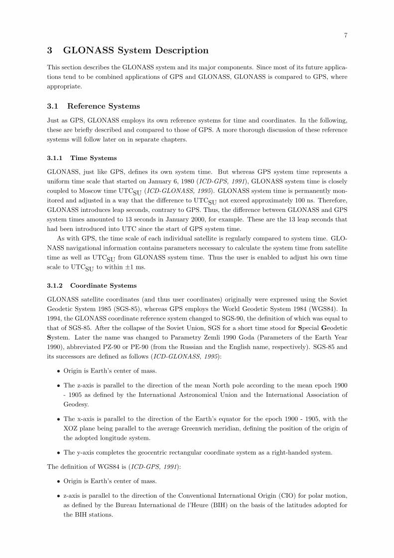
The ground segment consists of the System Control Center, the Central Synchronizer and the PhaseControl Center, which are all situated in Moscow. Seven additional ground stations are maintained inthe territory of the former Soviet Union, serving for orbit determination and satellite monitoring. Thesestations are equipped with radar, laser distance meters and/or telemetry. They are situated near thefollowing towns (see Figure 3.1):
St. Petersburg TT&CTernopol TT&C, laser ranging, monitoringJenisejsk TT&CKomsomol’sk-na-Amure TT&C, laser ranging, monitoringBalchas Laser rangingJevpatoria Laser rangingKitab Laser ranging
Only satellites over the northern hemisphere, exclusive large parts of North America, are visible fromthese stations. (Jansche, 1993). This lacking of a global coverage is a large handicap of the GLONASSsystem, since it may cause delays in the discovery of satellite anomalies and updating of satellite data.Therefore, during the development phase of GLONASS, ground stations were planned to be set up infellow socialist countries Cuba and Angola. But after the collapse of the Soviet Union, these plans werenot realized.
In order to determine the satellite orbits, satellites are tracked by radar 3 – 5 times for 10 – 15minutes each every 10 – 14 revolutions (Bartenev et al., 1994). By these means, the determination of the
3.3 Space Segment 9
Figure 3.1: Locations of GLONASS ground stations.
satellite positions is accomplished with an accuracy of approximately 2 – 3 m at the times of tracking.The radar data are regularly compared to the results of laser tracking of the satellites to calibrate theradar facilities. These laser range measurements yield accuracies near 1.5 – 2 cm in distance and 2 – 3”in angular coordinates. The equations of motion of the satellites are numerically integrated, consideringthe Earth’s gravitational potential as well as gravitational and non-gravitational disturbances, with themeasured satellite positions as initial values. Obtained solutions are extrapolated for up to 30 days anduploaded to the satellites, where they are stored. Error specifications for the GLONASS broadcast orbitsare given in Table 3.2.
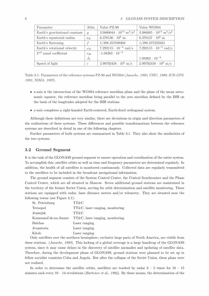
3.3 Space Segment
The GLONASS space segment consists of 24 satellites, distributed over three orbital planes. The longitudeof ascending node differs by 120◦ from plane to plane. Each plane comprises eight satellites, staggered
Mean square errorSatellite position vector Along track 20 m
Cross track 10 mRadial 5 m
Satellite velocity vector Along track 0.05 cm/sCross track 0.1 cm/sRadial 0.3 cm/s
Time scale synchronization 20 ns
Table 3.2: Mean square errors of GLONASS broadcast ephemerides (ICD-GLONASS, 1995).
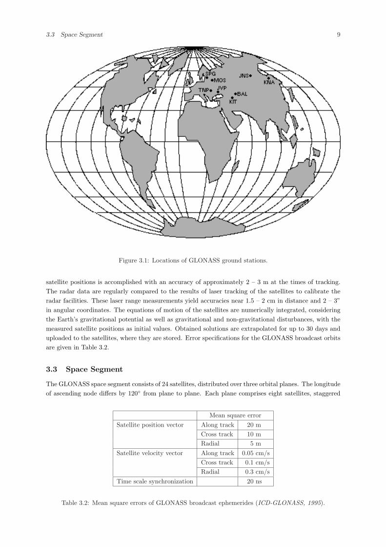
10 3 GLONASS SYSTEM DESCRIPTION
Parameter GLONASS GPSSemi-major axis 25510 km 26580 kmOrbital height 19130 km 20200 kmOrbital period 11 h 15.8 min 11 h 58 minInclination 64.8◦ 55◦
Eccentricity ≤0.01 ≤0.1Distinguishing between satellites FDMA CDMA
(1 code, multiple frequencies) (1 frequency, multiple codes)Frequencies L1 1602 - 1615.5 MHz 1575.42 MHz
L2 1246 - 1256.5 MHz 1227.60 MHzSignal polarization RHCP RHCP
Table 3.3: Parameters of the GLONASS and GPS space segments (ICD-GLONASS, 1995; ICD-GPS,1991).
by 45◦ in argument of latitude. The arguments of latitude of satellites in equivalent slots in two differentorbital planes differ by 15◦.
The GPS space segment also consists of nominally 24 satellites, which are, however, distributed oversix orbital planes, differing from plane to plane by 60◦ in longitude of the ascending node. Orbital andother parameters of the spacecraft are summarized in Table 3.3.
The orbital period of 11 h 15.8 min for GLONASS satellites means that for a stationary observerthe same satellite is visible at the same point in the sky every eight sidereal days. Since there are eightsatellites in each orbital plane, each day a different satellite appears at the same point in the sky. Withthe 11 h 58 min orbital period for GPS satellites, the same GPS satellite is visible at the same point inthe sky every (sidereal) day.
Besides its atomic clock and the equipment for receiving, processing, storing and transmitting navi-gational data, GLONASS satellites carry an extensive propulsion system, enabling the satellite to keepits orbital position, to control its attitude and even to manoeuvre to a different orbital position. Theattitude control system obtains its information from a number of different sensors, including an earthsensor and a magnetometer. Reflectors on the satellite body near the transmission antennae serve forpurposes of laser ranging from ground stations. The cylindrical body measures 2.35 m in diameter andmore than 3 m in length; overall length (with magnetometer boom unfolded) is 7.84 m. The solar arraysspan 7.23 m and include an area of 17.5 m2. They supply a total of 1.6 kW of electrical power. The massof a GLONASS satellite is approximately 1300 kg. The satellites launched in 1995 were second generationspacecraft (not to be confounded with GLONASS-M). They are already designed for a longer life time offive years and incorporate more stable frequency standards. Their mass is approximately 1410 kg, with23.6 m2 of solar panels for improved power supply (Johnson, 1994; Revnivykh and Mitrikas, 1998; CSIC,1998; Bartenev et al., 1994; Kazantsev, 1995; Gouzhva et al., 1995). A GLONASS satellite is depictedin Figure 3.2.
3.4 GLONASS Frequency Plan
To distinguish between individual satellites GLONASS satellites employ different frequencies to broadcasttheir navigational information. Satellite frequencies are determined by the equation
fL1 = 1602 + k · 0.5625 MHz L1 frequency andfL2 = 1246 + k · 0.4375 MHz L2 frequency.
In this equation, k means the frequency number of the satellite. The frequency domain as specifiedin Table 3.3 is equivalent to the frequency numbers 0 – 24. Frequency number 0 is the so-called technical

3.4 GLONASS Frequency Plan 11
Figure 3.2: GLONASS satellite (model displayed at 1997 Moscow Air Show, taken from (CDISS, 1998)).
frequency. It is reserved for testing purposes during the commissioning phase of a satellite. Numbers1 – 24 are assigned to operational satellites. The frequency ratio fL2/fL1 equals 7/9 for GLONASS. Thecorresponding frequency ratio for GPS is 60/77.
Originally, each of the 24 satellites was scheduled to have its own unique frequency number. Butpart of this GLONASS frequency spectrum also is important for radio astronomy. 1612 MHz (equallingGLONASS frequency number 18 in the L1 sub-band) is the frequency for radiation emitted by the 1 → 2transition in the quartet of 2Π 3
2, J = 3
2 state of hydroxyl (OH), a molecule common in interstellar clouds.The 1612 MHz line of hydroxyl in particular seems always to arise in the atmosphere of cool IR stars.Observation of hydroxyl molecules may provide vital clues about the evolution of our galaxy (Cook, 1977;Litvak, 1969; Verschuur and Kellermann, 1974). In addition, some providers of satellite communicationsservices (especially Motorola, Inc. for their Iridium system) started claiming other parts of the GLONASSfrequency band. At the World Administrative Radio Conference 1992, these satellite communicationsproviders were granted the right to share use of the upper portion of the GLONASS frequency band (from1610 MHz onwards) (N.N., 1992). (Meanwhile another agreement has been reached between Motorolaand radio astronomers regarding usage of the 1612 MHz.)
Therefore, beginning in 1993 the GLONASS frequency plan was re-organized in such a way thatantipodal satellites – i.e. satellites in opposing slots within the same orbital plane – share the samefrequency numbers, thus cutting to half the number of required frequencies. This sharing of frequenciesby antipodal satellites avoids unintentional mutual jamming of satellites at least for land, sea and airborneusers of the system. Spaceborne users above an orbital height of approximately 200 km, however, maysee both satellites transmitting on the same frequency at least during part of their orbits – cf. (Werner,1998).
This re-organization of the frequency plan is scheduled to take place in three stages. The first stagewas implemented from 1993 to 1998. It called for frequency sharing by antipodal satellites to avoid usageof frequency numbers 16 – 20 (1611.0 – 1613.25 MHz), thus clearing the 1612 MHz for radio astronomy.Frequency numbers 13, 14, 15 and 21 were to be used only under exceptional circumstances, frequencynumber 0 remained as technical frequency. This left frequency numbers 1 . . . 12, 22, 23 and 24 to beused for normal operation.
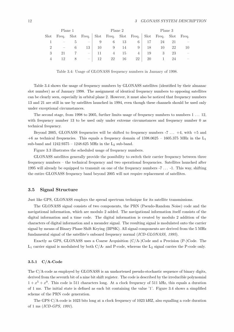
12 3 GLONASS SYSTEM DESCRIPTION
Plane 1 Plane 2 Plane 3Slot Freq. Slot Freq. Slot Freq. Slot Freq. Slot Freq. Slot Freq.
1 – 5 – 9 6 13 6 17 24 21 –2 – 6 13 10 9 14 9 18 10 22 103 21 7 – 11 4 15 4 19 3 23 –4 12 8 – 12 22 16 22 20 1 24 –
Table 3.4: Usage of GLONASS frequency numbers in January of 1998.
Table 3.4 shows the usage of frequency numbers by GLONASS satellites (identified by their almanacslot number) as of January 1998. The assignment of identical frequency numbers to opposing satellitescan be clearly seen, especially in orbital plane 2. However, it must also be noticed that frequency numbers13 and 21 are still in use by satellites launched in 1994, even though these channels should be used onlyunder exceptional circumstances.
The second stage, from 1998 to 2005, further limits usage of frequency numbers to numbers 1 . . . 12,with frequency number 13 to be used only under extreme circumstances and frequency number 0 astechnical frequency.
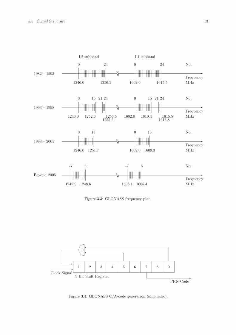
Beyond 2005, GLONASS frequencies will be shifted to frequency numbers -7 . . . +4, with +5 and+6 as technical frequencies. This equals a frequency domain of 1598.0625 – 1605.375 MHz in the L1
sub-band and 1242.9375 – 1248.625 MHz in the L2 sub-band.
Figure 3.3 illustrates the scheduled usage of frequency numbers.
GLONASS satellites generally provide the possibility to switch their carrier frequency between threefrequency numbers – the technical frequency and two operational frequencies. Satellites launched after1995 will already be equipped to transmit on one of the frequency numbers -7 . . . -1. This way, shiftingthe entire GLONASS frequency band beyond 2005 will not require replacement of satellites.
3.5 Signal Structure
Just like GPS, GLONASS employs the spread spectrum technique for its satellite transmissions.
The GLONASS signal consists of two components, the PRN (Pseudo-Random Noise) code and thenavigational information, which are modulo 2 added. The navigational information itself consists of thedigital information and a time code. The digital information is created by modulo 2 addition of thecharacters of digital information and a meander signal. The resulting signal is modulated onto the carriersignal by means of Binary Phase Shift Keying (BPSK). All signal components are derived from the 5 MHzfundamental signal of the satellite’s onboard frequency normal (ICD-GLONASS, 1995).
Exactly as GPS, GLONASS uses a Coarse Acquisition (C/A-)Code and a Precision (P-)Code. TheL1 carrier signal is modulated by both C/A- and P-code, whereas the L2 signal carries the P-code only.
3.5.1 C/A-Code
The C/A-code as employed by GLONASS is an unshortened pseudo-stochastic sequence of binary digits,derived from the seventh bit of a nine bit shift register. The code is described by the irreducible polynomial1 + x5 + x9. This code is 511 characters long. At a clock frequency of 511 kHz, this equals a durationof 1 ms. The initial state is defined as each bit containing the value ’1’. Figure 3.4 shows a simplifiedscheme of the PRN code generation.
The GPS C/A-code is 1023 bits long at a clock frequency of 1023 kHZ, also equalling a code durationof 1 ms (ICD-GPS, 1991).
3.5 Signal Structure 13
L2 subband L1 subband
1982 – 1993 -FrequencyMHz
No.0
1602.0
24
1615.5
0
1246.0
24
1256.5
1993 – 1998 -FrequencyMHz
No.0
1602.0
15
1610.4
21
1613.8
24
1615.5
0
1246.0
15
1252.6
21
1255.2
24
1256.5
1998 – 2005 -FrequencyMHz
No.0
1602.0
13
1609.3
0
1246.0
13
1251.7
Beyond 2005 -FrequencyMHz
No.-7
1598.1
6
1605.4
-7
1242.9
6
1248.6
Figure 3.3: GLONASS frequency plan.
-Clock Signal
9 Bit Shift Register
1 2 3 4 5 6 7 8 9
¾¾
¾
½⊕
-
-PRN Code
Figure 3.4: GLONASS C/A-code generation (schematic).
14 3 GLONASS SYSTEM DESCRIPTION
-Clock Signal
25 Bit Shift Register
1 2 3 4 5 6 7 8 9 10 11 12 13 14 15 16 17 18 19 20 21 22 23 24 25
¾¾
¾
½⊕
-
-PRN Code
- / 5,110,000
-
Reset
Figure 3.5: GLONASS P-code generation (schematic).
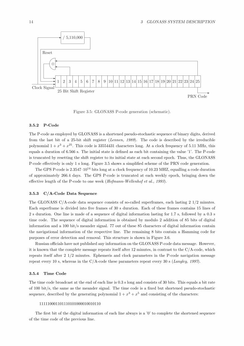
3.5.2 P-Code
The P-code as employed by GLONASS is a shortened pseudo-stochastic sequence of binary digits, derivedfrom the last bit of a 25-bit shift register (Lennen, 1989). The code is described by the irreduciblepolynomial 1 + x3 + x25. This code is 33554431 characters long. At a clock frequency of 5.11 MHz, thisequals a duration of 6.566 s. The initial state is defined as each bit containing the value ’1’. The P-codeis truncated by resetting the shift register to its initial state at each second epoch. Thus, the GLONASSP-code effectively is only 1 s long. Figure 3.5 shows a simplified scheme of the PRN code generation.
The GPS P-code is 2.3547 ·1014 bits long at a clock frequency of 10.23 MHZ, equalling a code durationof approximately 266.4 days. The GPS P-code is truncated at each weekly epoch, bringing down theeffective length of the P-code to one week (Hofmann-Wellenhof et al., 1993).
3.5.3 C/A-Code Data Sequence
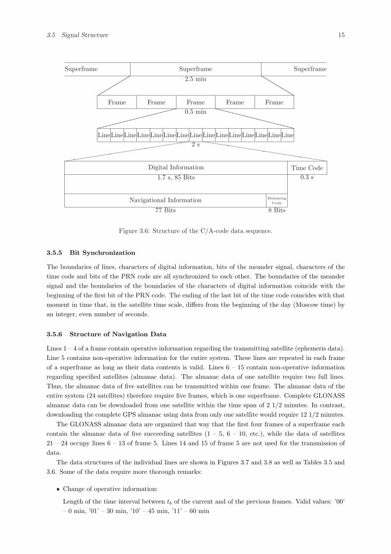
The GLONASS C/A-code data sequence consists of so-called superframes, each lasting 2 1/2 minutes.Each superframe is divided into five frames of 30 s duration. Each of these frames contains 15 lines of2 s duration. One line is made of a sequence of digital information lasting for 1.7 s, followed by a 0.3 stime code. The sequence of digital information is obtained by modulo 2 addition of 85 bits of digitalinformation and a 100 bit/s meander signal. 77 out of these 85 characters of digital information containthe navigational information of the respective line. The remaining 8 bits contain a Hamming code forpurposes of error detection and removal. This structure is shown in Figure 3.6.
Russian officials have not published any information on the GLONASS P-code data message. However,it is known that the complete message repeats itself after 12 minutes, in contrast to the C/A-code, whichrepeats itself after 2 1/2 minutes. Ephemeris and clock parameters in the P-code navigation messagerepeat every 10 s, whereas in the C/A-code these parameters repeat every 30 s (Langley, 1997).
3.5.4 Time Code
The time code broadcast at the end of each line is 0.3 s long and consists of 30 bits. This equals a bit rateof 100 bit/s, the same as the meander signal. The time code is a fixed but shortened pseudo-stochasticsequence, described by the generating polynomial 1 + x3 + x5 and consisting of the characters:
111110001101110101000010010110
The first bit of the digital information of each line always is a ’0’ to complete the shortened sequenceof the time code of the previous line.
3.5 Signal Structure 15
Navigational Information HammingCode
77 Bits 8 Bits
Digital Information Time Code1.7 s, 85 Bits 0.3 s
LineLineLineLineLineLineLineLineLineLineLineLineLineLineLine2 s
Frame Frame Frame Frame Frame0.5 min
Superframe Superframe Superframe2.5 min
Figure 3.6: Structure of the C/A-code data sequence.
3.5.5 Bit Synchronization
The boundaries of lines, characters of digital information, bits of the meander signal, characters of thetime code and bits of the PRN code are all synchronized to each other. The boundaries of the meandersignal and the boundaries of the boundaries of the characters of digital information coincide with thebeginning of the first bit of the PRN code. The ending of the last bit of the time code coincides with thatmoment in time that, in the satellite time scale, differs from the beginning of the day (Moscow time) byan integer, even number of seconds.
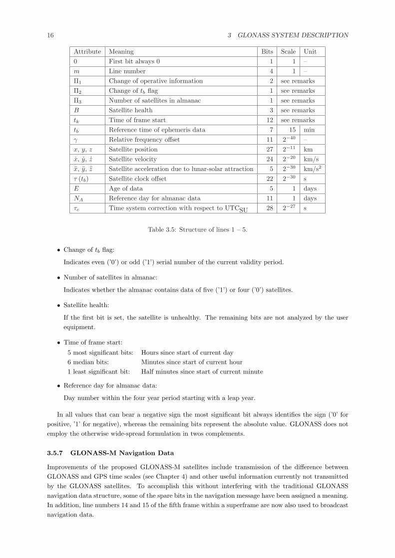
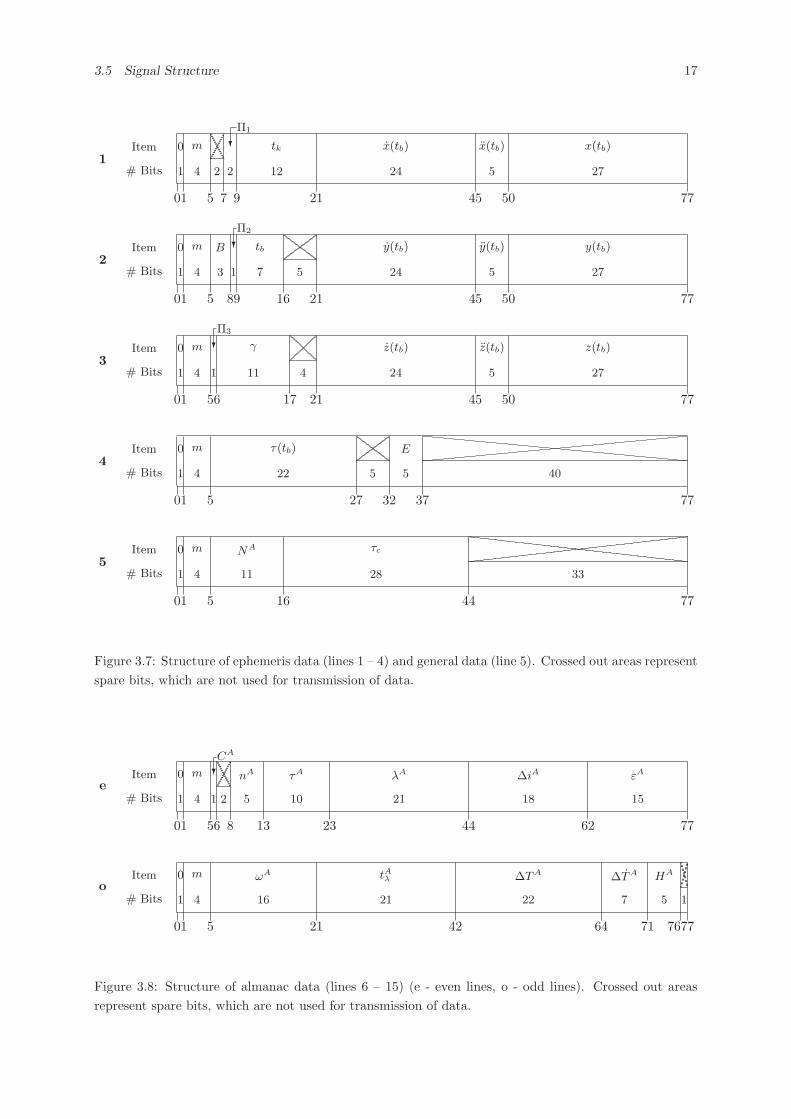
3.5.6 Structure of Navigation Data
Lines 1 – 4 of a frame contain operative information regarding the transmitting satellite (ephemeris data).Line 5 contains non-operative information for the entire system. These lines are repeated in each frameof a superframe as long as their data contents is valid. Lines 6 – 15 contain non-operative informationregarding specified satellites (almanac data). The almanac data of one satellite require two full lines.Thus, the almanac data of five satellites can be transmitted within one frame. The almanac data of theentire system (24 satellites) therefore require five frames, which is one superframe. Complete GLONASSalmanac data can be downloaded from one satellite within the time span of 2 1/2 minutes. In contrast,downloading the complete GPS almanac using data from only one satellite would require 12 1/2 minutes.
The GLONASS almanac data are organized that way that the first four frames of a superframe eachcontain the almanac data of five succeeding satellites (1 – 5, 6 – 10, etc.), while the data of satellites21 – 24 occupy lines 6 – 13 of frame 5. Lines 14 and 15 of frame 5 are not used for the transmission ofdata.
The data structures of the individual lines are shown in Figures 3.7 and 3.8 as well as Tables 3.5 and3.6. Some of the data require more thorough remarks:
• Change of operative information:
Length of the time interval between tb of the current and of the previous frames. Valid values: ’00’– 0 min, ’01’ – 30 min, ’10’ – 45 min, ’11’ – 60 min
16 3 GLONASS SYSTEM DESCRIPTION
Attribute Meaning Bits Scale Unit0 First bit always 0 1 1 –m Line number 4 1 –Π1 Change of operative information 2 see remarksΠ2 Change of tb flag 1 see remarksΠ3 Number of satellites in almanac 1 see remarksB Satellite health 3 see remarkstk Time of frame start 12 see remarkstb Reference time of ephemeris data 7 15 minγ Relative frequency offset 11 2−40 –x, y, z Satellite position 27 2−11 kmx, y, z Satellite velocity 24 2−20 km/sx, y, z Satellite acceleration due to lunar-solar attraction 5 2−30 km/s2
τ (tb) Satellite clock offset 22 2−30 sE Age of data 5 1 daysNA Reference day for almanac data 11 1 daysτc Time system correction with respect to UTCSU 28 2−27 s
Table 3.5: Structure of lines 1 – 5.
• Change of tb flag:
Indicates even (’0’) or odd (’1’) serial number of the current validity period.
• Number of satellites in almanac:
Indicates whether the almanac contains data of five (’1’) or four (’0’) satellites.
• Satellite health:
If the first bit is set, the satellite is unhealthy. The remaining bits are not analyzed by the userequipment.
• Time of frame start:
5 most significant bits: Hours since start of current day6 median bits: Minutes since start of current hour1 least significant bit: Half minutes since start of current minute
• Reference day for almanac data:
Day number within the four year period starting with a leap year.
In all values that can bear a negative sign the most significant bit always identifies the sign (’0’ forpositive, ’1’ for negative), whereas the remaining bits represent the absolute value. GLONASS does notemploy the otherwise wide-spread formulation in twos complements.
3.5.7 GLONASS-M Navigation Data
Improvements of the proposed GLONASS-M satellites include transmission of the difference betweenGLONASS and GPS time scales (see Chapter 4) and other useful information currently not transmittedby the GLONASS satellites. To accomplish this without interfering with the traditional GLONASSnavigation data structure, some of the spare bits in the navigation message have been assigned a meaning.In addition, line numbers 14 and 15 of the fifth frame within a superframe are now also used to broadcastnavigation data.
3.5 Signal Structure 17
1# Bits
Item
0 771
1
0
5
4
m
7
2
9
2
Π1
?
21
12
tk
45
24
x(tb)
50
5
x(tb)
27
x(tb)
2# Bits
Item
0 771
1
0
5
4
m
8
3
B
9
1
Π2
?
16
7
tb
21
5
45
24
y(tb)
50
5
y(tb)
27
y(tb)
3# Bits
Item
0 771
1
0
5
4
m
6
1
Π3
?
17
11
γ
21
4
45
24
z(tb)
50
5
z(tb)
27
z(tb)
4# Bits
Item
0 771
1
0
5
4
m
27
22
τ(tb)
32
5
37
5
E
40
5# Bits
Item
0 771
1
0
5
4
m
16
11
NA
44
28
τc
33
Figure 3.7: Structure of ephemeris data (lines 1 – 4) and general data (line 5). Crossed out areas representspare bits, which are not used for transmission of data.
e# Bits
Item
0 771
1
0
5
4
m
6
1
CA
?
8
2
13
5
nA
23
10
τA
44
21
λA
62
18
∆iA
15
εA
o# Bits
Item
0 771
1
0
5
4
m
21
16
ωA
42
21
tAλ
64
22
∆T A
71
7
∆T A
76
5
HA
1
Figure 3.8: Structure of almanac data (lines 6 – 15) (e - even lines, o - odd lines). Crossed out areasrepresent spare bits, which are not used for transmission of data.
18 3 GLONASS SYSTEM DESCRIPTION
Attribute Meaning Bits Scale Unit0 First bit always 0 1 1 –m Line number 4 1 –nA Satellite slot number 5 1 –CA Satellite health 1 0 = no, 1 = yesτA Satellite clock offset 10 2−18 sλA Greenwich longitude of first equator crossing 21 2−20 semi-circles∆iA Correction to nominal inclination 18 2−20 semi-circlesεA Eccentricity 15 2−20 –ωA Argument of perigee 16 2−15 semi-circlestAλ Time of first equator crossing 21 2−5 s∆TA Correction to nominal orbital period 22 2−9 s∆TA Rate of change of orbital period 7 2−14 s/orbitHA Satellite frequency number 5 1 –
Table 3.6: Structure of lines 6 – 15.
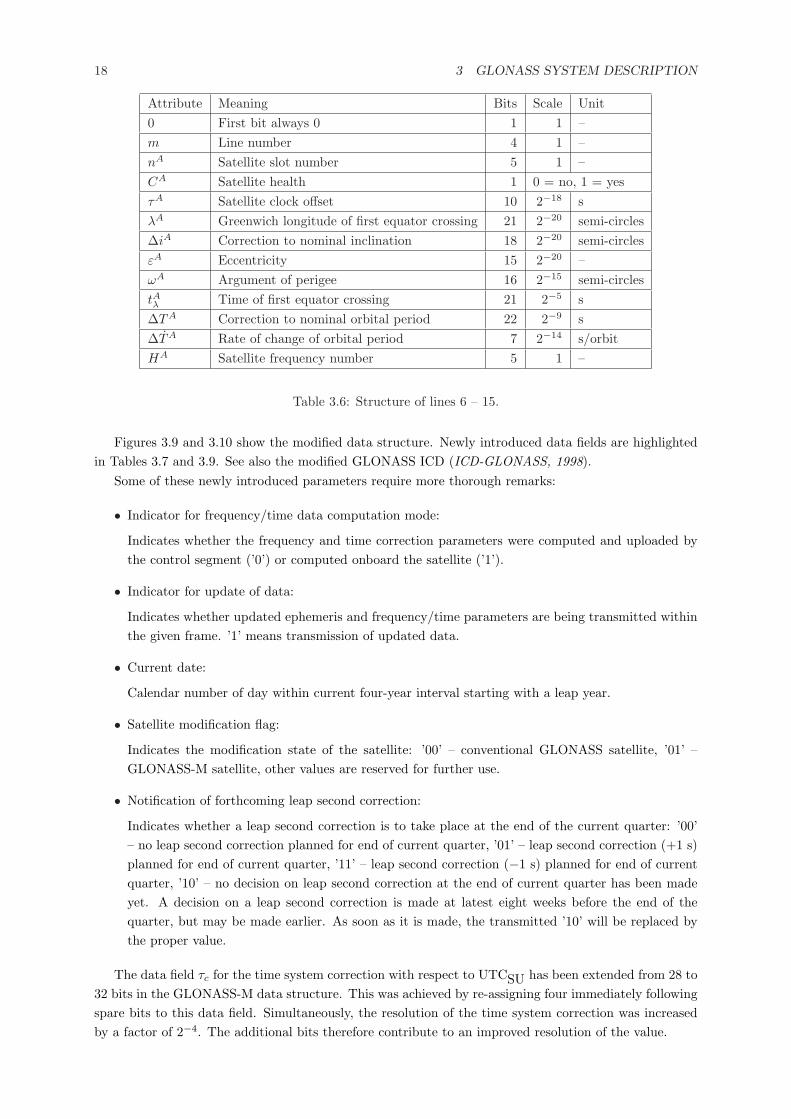
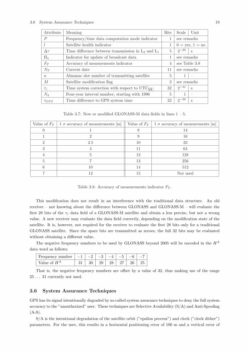
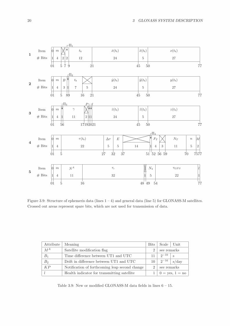
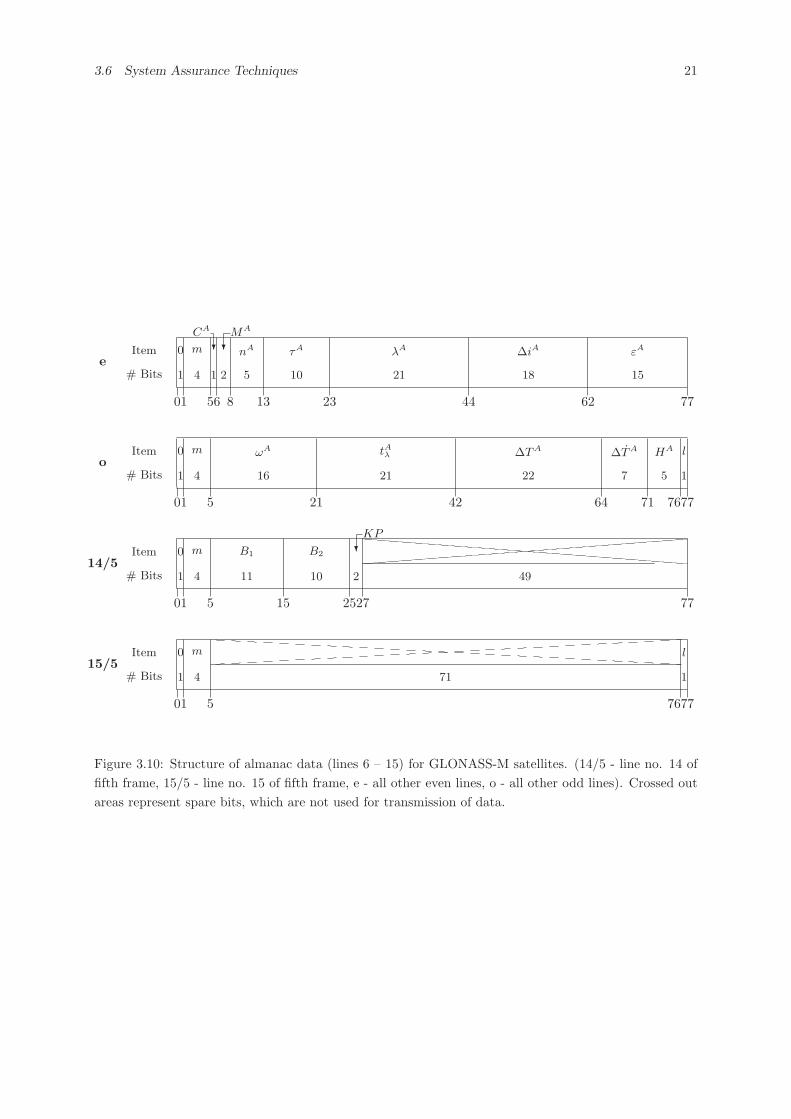
Figures 3.9 and 3.10 show the modified data structure. Newly introduced data fields are highlightedin Tables 3.7 and 3.9. See also the modified GLONASS ICD (ICD-GLONASS, 1998).
Some of these newly introduced parameters require more thorough remarks:
• Indicator for frequency/time data computation mode:
Indicates whether the frequency and time correction parameters were computed and uploaded bythe control segment (’0’) or computed onboard the satellite (’1’).
• Indicator for update of data:
Indicates whether updated ephemeris and frequency/time parameters are being transmitted withinthe given frame. ’1’ means transmission of updated data.
• Current date:
Calendar number of day within current four-year interval starting with a leap year.
• Satellite modification flag:
Indicates the modification state of the satellite: ’00’ – conventional GLONASS satellite, ’01’ –GLONASS-M satellite, other values are reserved for further use.
• Notification of forthcoming leap second correction:
Indicates whether a leap second correction is to take place at the end of the current quarter: ’00’– no leap second correction planned for end of current quarter, ’01’ – leap second correction (+1 s)planned for end of current quarter, ’11’ – leap second correction (−1 s) planned for end of currentquarter, ’10’ – no decision on leap second correction at the end of current quarter has been madeyet. A decision on a leap second correction is made at latest eight weeks before the end of thequarter, but may be made earlier. As soon as it is made, the transmitted ’10’ will be replaced bythe proper value.
The data field τc for the time system correction with respect to UTCSU has been extended from 28 to32 bits in the GLONASS-M data structure. This was achieved by re-assigning four immediately followingspare bits to this data field. Simultaneously, the resolution of the time system correction was increasedby a factor of 2−4. The additional bits therefore contribute to an improved resolution of the value.
3.6 System Assurance Techniques 19
Attribute Meaning Bits Scale UnitP Frequency/time data computation mode indicator 1 see remarksl Satellite health indicator 1 0 = yes, 1 = no∆τ Time difference between transmission in L2 and L1 5 2−30 sΠ4 Indicator for update of broadcast data 1 see remarksFT Accuracy of measurements indicator 4 see Table 3.8NT Current date 11 see remarksn Almanac slot number of transmitting satellite 5 1 –M Satellite modification flag 2 see remarksτc Time system correction with respect to UTCSU 32 2−31 sN4 Four-year interval number, starting with 1996 5 1 –τGPS Time difference to GPS system time 22 2−30 s
Table 3.7: New or modified GLONASS-M data fields in lines 1 – 5.
Value of FT 1 σ accuracy of measurements [m] Value of FT 1 σ accuracy of measurements [m]0 1 8 141 2 9 162 2.5 10 323 4 11 644 5 12 1285 7 13 2566 10 14 5127 12 15 Not used
Table 3.8: Accuracy of measurements indicator FT .
This modification does not result in an interference with the traditional data structure. An oldreceiver – not knowing about the difference between GLONASS and GLONASS-M – will evaluate thefirst 28 bits of the τc data field of a GLONASS-M satellite and obtain a less precise, but not a wrongvalue. A new receiver may evaluate the data field correctly, depending on the modification state of thesatellite. It is, however, not required for the receiver to evaluate the first 28 bits only for a traditionalGLONASS satellite. Since the spare bits are transmitted as zeroes, the full 32 bits may be evaluatedwithout obtaining a different value.
The negative frequency numbers to be used by GLONASS beyond 2005 will be encoded in the HA
data word as follows:
Frequency number −1 −2 −3 −4 −5 −6 −7Value of HA 31 30 29 28 27 26 25
That is, the negative frequency numbers are offset by a value of 32, thus making use of the range25 . . . 31 currently not used.
3.6 System Assurance Techniques
GPS has its signal intentionally degraded by so-called system assurance techniques to deny the full systemaccuracy to the ”unauthorized” user. These techniques are Selective Availability (S/A) and Anti-Spoofing(A-S).
S/A is the intentional degradation of the satellite orbit (”epsilon process”) and clock (”clock dither”)parameters. For the user, this results in a horizontal positioning error of 100 m and a vertical error of
20 3 GLONASS SYSTEM DESCRIPTION
1# Bits
Item
0 771
1
0
5
4
m
7
2
9
2
Π1
?
21
12
tk
45
24
x(tb)
50
5
x(tb)
27
x(tb)
2# Bits
Item
0 771
1
0
5
4
m
8
3
B
9
1
Π2
?
16
7
tb
21
5
45
24
y(tb)
50
5
y(tb)
27
y(tb)
3# Bits
Item
0 771
1
0
5
4
m
6
1
Π3
?
17
11
γ
19
2
20
1
P?
21
1
l?
45
24
z(tb)
50
5
z(tb)
27
z(tb)
4# Bits
Item
0 771
1
0
5
4
m
27
22
τ(tb)
32
5
∆τ
37
5
E
51
14
52
1
Π4
?
56
4
FT
59
3
70
11
NT
75
5
n
2
M
5# Bits
Item
0 771
1
0
5
4
m
16
11
NA
48
32
τc
49
1
54
5
N4
22
τGPS
1
l
Figure 3.9: Structure of ephemeris data (lines 1 – 4) and general data (line 5) for GLONASS-M satellites.Crossed out areas represent spare bits, which are not used for transmission of data.
Attribute Meaning Bits Scale UnitMA Satellite modification flag 2 see remarksB1 Time difference between UT1 and UTC 11 2−10 sB2 Drift in difference between UT1 and UTC 10 2−16 s/dayKP Notification of forthcoming leap second change 2 see remarksl Health indicator for transmitting satellite 1 0 = yes, 1 = no
Table 3.9: New or modified GLONASS-M data fields in lines 6 – 15.
3.6 System Assurance Techniques 21
e# Bits
Item
0 771
1
0
5
4
m
6
1
CA
?
8
2
MA
?
13
5
nA
23
10
τA
44
21
λA
62
18
∆iA
15
εA
o# Bits
Item
0 771
1
0
5
4
m
21
16
ωA
42
21
tAλ
64
22
∆T A
71
7
∆T A
76
5
HA
1
l
14/5# Bits
Item
0 771
1
0
5
4
m
15
11
B1
25
10
B2
27
2
KP?
49
15/5# Bits
Item
0 771
1
0
5
4
m
76
71 1
l
Figure 3.10: Structure of almanac data (lines 6 – 15) for GLONASS-M satellites. (14/5 - line no. 14 offifth frame, 15/5 - line no. 15 of fifth frame, e - all other even lines, o - all other odd lines). Crossed outareas represent spare bits, which are not used for transmission of data.
22 3 GLONASS SYSTEM DESCRIPTION
Position Deviation [m] from Center E 11� 37’ 41.901” N 48� 04’ 40.912”
East/West Deviation [m]
-50 -40 -30 -20 -10 0 10 20 30 40 50
Nor
th/S
outh
Dev
iati
on[m
]
-50
-40
-30
-20
-10
0
10
20
30
40
50
◦◦◦◦◦◦◦◦
◦
◦◦◦
◦
◦◦◦◦
◦◦◦◦
◦◦
◦◦◦
◦◦
◦
◦◦◦◦◦◦◦◦
◦
◦◦◦◦◦◦◦◦◦◦◦
◦◦◦◦◦◦◦◦◦
◦◦◦◦
◦
◦◦◦◦◦◦◦
◦
◦
◦◦◦◦◦◦◦◦◦◦◦◦◦◦◦◦◦◦◦◦◦◦◦◦◦◦◦◦◦◦◦◦◦◦◦◦◦◦◦◦◦◦◦◦◦◦◦◦◦◦◦◦◦◦◦◦◦◦◦◦◦◦◦◦◦◦◦◦◦◦◦◦◦◦◦◦◦◦◦◦◦◦◦◦◦◦◦◦◦◦◦◦◦◦◦◦◦◦◦◦◦◦◦◦◦◦◦◦◦◦◦◦◦◦◦◦◦◦◦◦◦◦◦◦◦◦◦◦◦◦◦◦◦◦◦◦◦◦◦◦◦◦◦◦◦◦◦◦◦◦◦◦◦◦◦◦◦◦◦◦◦◦◦◦◦◦◦
◦◦◦
◦◦◦◦◦◦◦◦◦◦
◦◦◦◦◦◦◦◦◦◦◦◦◦◦◦◦◦◦◦◦◦◦◦◦◦
◦◦
◦
◦◦
◦◦
◦◦
◦
◦◦◦◦◦◦◦◦◦◦◦◦◦◦◦◦◦◦◦◦
◦
◦◦◦◦◦◦◦◦◦◦◦◦◦◦◦◦◦◦◦◦◦◦◦◦◦◦◦◦◦◦◦◦◦◦◦◦◦◦◦◦◦◦◦◦◦◦◦◦◦◦◦◦◦◦◦◦◦◦◦◦◦◦◦◦◦◦◦◦◦◦◦◦◦◦◦◦◦◦◦◦◦◦◦◦◦◦◦◦◦◦◦◦◦◦◦◦◦◦◦◦◦◦◦◦◦◦◦◦◦◦◦◦◦◦◦◦◦◦◦◦◦◦◦◦◦◦◦◦◦◦◦◦◦◦◦◦◦◦◦◦◦◦◦◦◦◦◦◦◦◦◦◦◦◦◦◦◦◦◦◦◦◦◦◦◦
◦◦◦◦◦◦◦◦◦◦◦◦◦◦◦◦◦◦◦◦◦◦◦◦◦◦◦◦◦◦◦◦◦◦◦◦◦◦◦◦◦◦◦◦◦◦◦◦◦◦◦◦◦◦◦◦◦◦◦◦◦◦◦◦◦◦◦◦◦◦◦◦◦◦◦◦◦◦◦◦◦◦◦◦◦◦◦◦◦◦◦◦◦◦◦◦◦◦◦◦◦◦◦◦◦◦◦◦◦◦◦◦◦◦◦◦◦◦◦◦◦◦◦◦◦◦◦◦◦◦◦◦◦◦◦◦◦◦◦◦◦◦◦◦◦◦◦◦◦◦◦◦◦◦◦◦◦◦◦◦◦◦◦◦◦◦◦◦◦◦◦◦◦◦◦◦◦◦◦◦◦◦◦◦◦◦◦◦◦◦◦◦◦◦◦◦◦◦◦◦◦◦◦◦◦◦◦◦◦◦◦◦◦◦◦◦◦◦◦◦◦◦◦◦◦◦◦◦◦◦◦◦◦◦◦◦◦◦◦◦◦◦◦◦◦◦◦◦◦◦◦◦◦◦◦◦◦◦◦◦◦◦◦◦◦◦◦◦◦◦◦◦◦◦◦◦◦◦◦◦◦◦◦◦◦◦◦◦◦◦◦◦◦◦◦◦◦◦◦◦◦◦◦◦◦◦◦◦◦◦◦◦◦◦◦◦◦◦◦◦◦◦◦◦◦◦◦◦◦◦◦◦◦◦◦◦◦◦◦◦◦◦◦◦◦◦◦◦◦◦◦◦◦◦◦◦◦◦◦◦◦◦◦◦◦◦◦◦◦◦
◦◦◦◦◦◦◦◦◦◦◦◦◦◦◦◦◦◦◦◦◦◦◦◦◦◦◦◦◦◦◦
◦◦◦◦◦◦◦◦◦◦◦◦◦◦◦◦◦◦◦◦◦◦◦◦◦◦◦◦◦◦◦◦◦◦◦◦◦◦◦◦◦◦◦◦◦◦◦◦◦◦◦◦◦◦◦◦◦◦◦◦◦◦◦◦◦◦◦◦◦◦◦◦◦◦◦◦◦◦◦◦◦◦◦◦◦◦◦◦◦◦◦◦◦◦◦◦◦◦◦◦◦◦◦◦◦◦◦◦◦◦◦◦◦◦◦◦◦◦◦◦◦◦◦◦◦◦◦◦◦◦◦◦◦◦◦◦◦◦◦◦◦◦◦◦◦◦◦◦◦◦◦◦◦◦◦◦◦◦◦◦◦◦◦◦◦◦◦◦◦◦◦◦◦◦◦◦◦◦◦◦◦◦◦◦◦◦◦◦◦◦◦◦◦◦◦◦◦◦◦◦◦◦◦◦◦◦◦◦◦◦◦◦◦◦◦◦◦◦◦◦◦◦◦◦◦◦◦◦◦◦◦◦◦◦◦◦◦◦◦◦◦◦◦◦◦◦◦◦◦◦◦◦◦◦◦◦◦◦◦◦◦◦◦◦◦◦◦◦◦◦◦◦◦◦◦◦◦◦◦◦◦◦◦◦◦◦◦◦◦◦◦◦◦◦◦◦◦◦◦◦◦◦◦◦◦◦◦◦◦◦◦◦◦◦◦◦◦◦◦◦◦◦◦◦◦◦◦◦◦◦◦◦◦◦◦◦◦◦◦◦◦◦◦◦◦◦◦◦◦◦◦◦◦◦◦◦◦◦◦◦◦◦◦◦◦◦◦◦◦◦◦◦◦◦◦◦◦◦◦◦◦◦◦◦◦◦◦◦◦◦◦◦◦◦◦◦◦◦◦◦◦◦◦◦◦◦◦◦◦◦◦◦◦◦◦◦◦◦◦◦◦◦◦◦◦◦◦◦◦◦◦◦◦◦◦◦◦◦◦◦◦◦◦◦◦◦◦◦◦◦◦◦◦◦◦◦◦◦◦◦◦◦◦◦◦◦◦◦◦◦◦◦◦◦◦◦◦◦◦◦◦◦◦◦◦◦◦◦◦◦◦◦◦◦◦◦◦◦◦◦◦◦◦◦◦◦◦◦◦◦◦◦◦◦◦◦◦◦◦◦◦◦◦◦◦◦◦◦◦◦◦◦◦◦◦◦◦◦◦◦◦◦◦◦◦◦◦◦◦◦◦◦◦◦◦◦◦◦◦◦◦◦◦◦◦◦◦◦◦◦◦◦◦◦◦◦◦◦◦◦◦◦◦◦◦◦◦◦◦◦◦◦◦◦◦◦◦◦◦◦◦◦◦◦◦◦◦◦◦◦◦◦◦◦◦◦◦◦◦◦◦◦◦◦◦◦◦◦◦◦◦◦◦◦◦◦◦◦◦◦◦◦◦◦◦◦◦◦◦◦◦◦◦◦◦◦◦◦◦◦◦◦◦◦◦◦◦◦◦◦◦◦◦◦◦◦◦◦◦◦◦◦◦◦◦◦◦◦◦◦◦◦◦◦◦◦◦◦◦◦◦◦◦◦◦◦◦◦◦◦◦◦◦◦◦◦◦◦◦◦◦◦◦◦◦◦◦◦◦◦◦◦◦◦◦◦◦◦◦◦◦◦◦◦◦◦◦◦◦◦◦◦◦◦◦◦◦◦◦◦◦◦◦◦◦◦◦◦◦◦◦◦◦◦◦◦◦◦◦◦◦◦◦◦◦◦◦◦◦◦◦◦◦◦◦◦◦◦◦◦◦◦◦◦◦◦◦◦◦◦◦◦◦◦◦◦◦◦◦◦◦◦◦◦◦◦◦◦◦◦◦◦◦◦◦◦◦◦◦◦◦◦◦◦◦◦◦◦◦◦◦◦◦◦◦◦◦◦◦◦◦◦◦◦◦◦◦◦◦◦◦◦◦◦◦◦◦◦◦◦◦◦◦◦◦◦◦◦◦◦◦◦◦◦◦◦◦◦◦◦◦◦◦◦◦◦◦◦◦◦◦◦◦◦◦◦◦◦◦◦◦◦◦
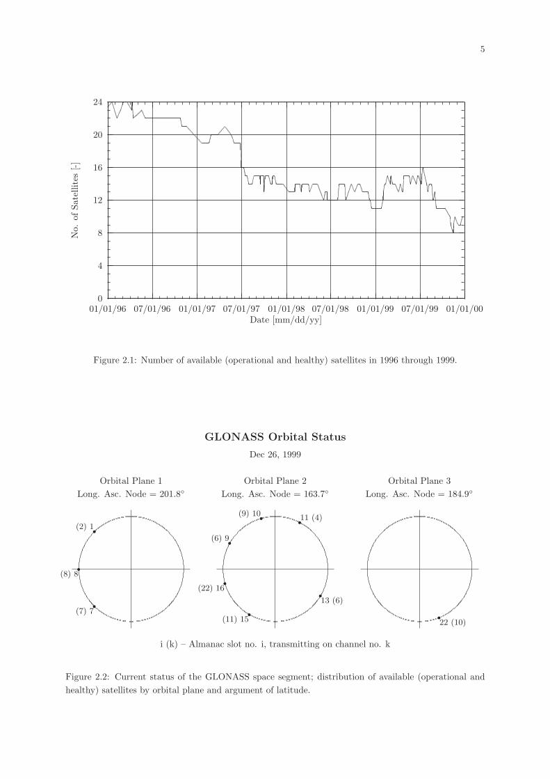
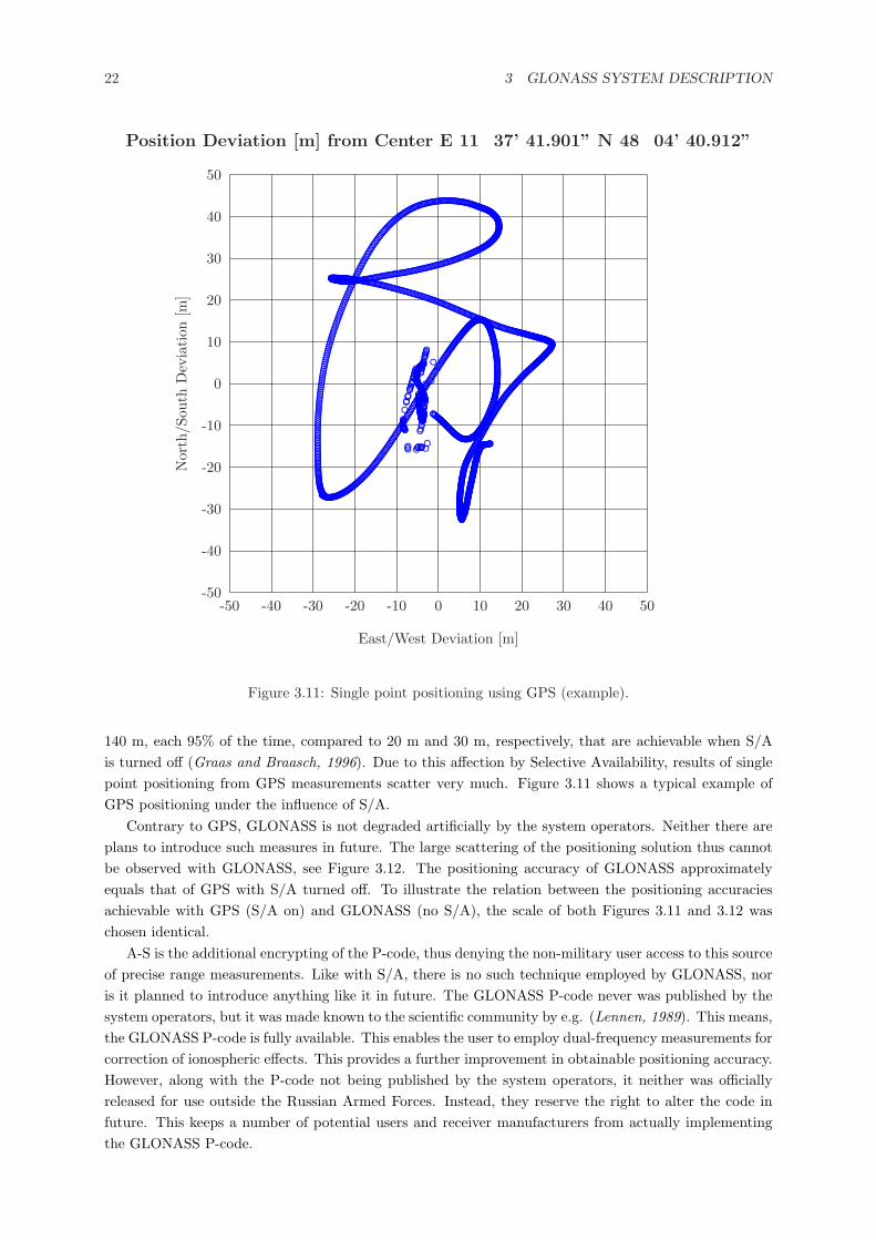
Figure 3.11: Single point positioning using GPS (example).
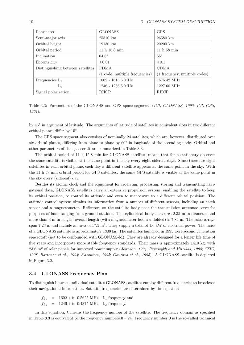
140 m, each 95% of the time, compared to 20 m and 30 m, respectively, that are achievable when S/Ais turned off (Graas and Braasch, 1996). Due to this affection by Selective Availability, results of singlepoint positioning from GPS measurements scatter very much. Figure 3.11 shows a typical example ofGPS positioning under the influence of S/A.
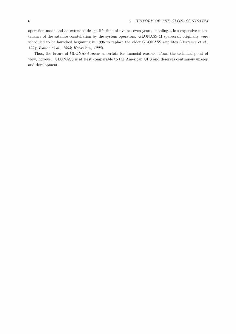
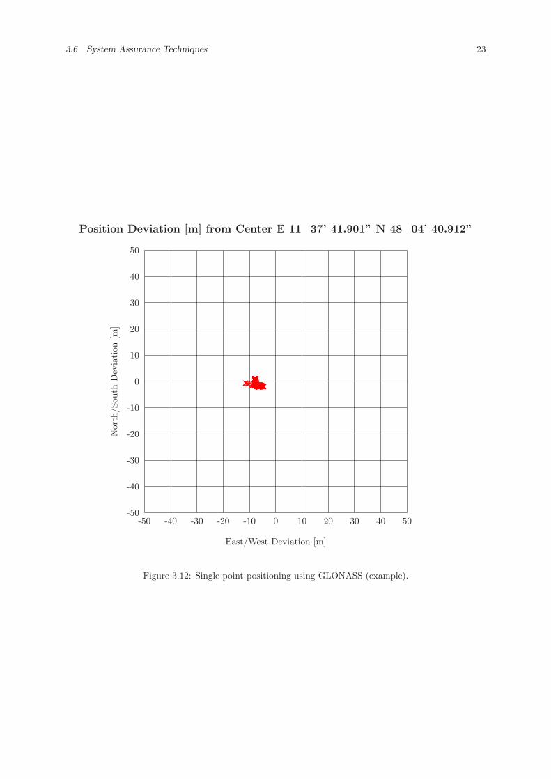
Contrary to GPS, GLONASS is not degraded artificially by the system operators. Neither there areplans to introduce such measures in future. The large scattering of the positioning solution thus cannotbe observed with GLONASS, see Figure 3.12. The positioning accuracy of GLONASS approximatelyequals that of GPS with S/A turned off. To illustrate the relation between the positioning accuraciesachievable with GPS (S/A on) and GLONASS (no S/A), the scale of both Figures 3.11 and 3.12 waschosen identical.
A-S is the additional encrypting of the P-code, thus denying the non-military user access to this sourceof precise range measurements. Like with S/A, there is no such technique employed by GLONASS, noris it planned to introduce anything like it in future. The GLONASS P-code never was published by thesystem operators, but it was made known to the scientific community by e.g. (Lennen, 1989). This means,the GLONASS P-code is fully available. This enables the user to employ dual-frequency measurements forcorrection of ionospheric effects. This provides a further improvement in obtainable positioning accuracy.However, along with the P-code not being published by the system operators, it neither was officiallyreleased for use outside the Russian Armed Forces. Instead, they reserve the right to alter the code infuture. This keeps a number of potential users and receiver manufacturers from actually implementingthe GLONASS P-code.
3.6 System Assurance Techniques 23
Position Deviation [m] from Center E 11� 37’ 41.901” N 48� 04’ 40.912”
East/West Deviation [m]
-50 -40 -30 -20 -10 0 10 20 30 40 50
Nor
th/S
outh
Dev
iati
on[m
]
-50
-40
-30
-20
-10
0
10
20
30
40
50
××××××××××××××××××××××××××××××××××××××××××××××××××××××××××××××××××××××××××××××××××××××××××××××××××××××××××××××××××××××××××××××××××××××××××××××××××××××××××××××××××××××××××××××××××××××××××××××××××××××××××××××××××××××××××××××××××××××××××××××××××××××××××××××××××××××××××××××××××××××××××××××××××××××××××××××××××××××××××××××××××××××××××××××××××××××××××××××××××××××××××××××××××××××××××××××××××××××××××××××××××××××××××××××××××××××××××××××××××××××××××××××××××××××××××××××××××××××××××××××××××××××××××××××××××× ××××××××××××××××××××××××××××××××××××××××××××××××××××××××××××××××××××××××××××××××××××××××××××××××××××××××××××××××××××××××××××××××××××××××××××××××××××××××××××××××××××××××××××××××××××××××××××××××××××××××××××××××××××××××××××××××××××××××××××××××××××××××××××××××××××××××××××××××××××××××××××××××××××××××××××××××××××××
Figure 3.12: Single point positioning using GLONASS (example).
24 3 GLONASS SYSTEM DESCRIPTION
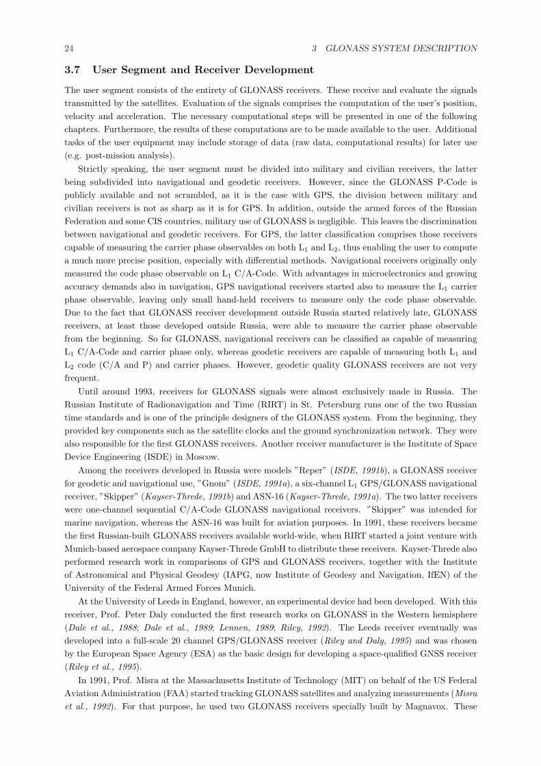
3.7 User Segment and Receiver Development
The user segment consists of the entirety of GLONASS receivers. These receive and evaluate the signalstransmitted by the satellites. Evaluation of the signals comprises the computation of the user’s position,velocity and acceleration. The necessary computational steps will be presented in one of the followingchapters. Furthermore, the results of these computations are to be made available to the user. Additionaltasks of the user equipment may include storage of data (raw data, computational results) for later use(e.g. post-mission analysis).
Strictly speaking, the user segment must be divided into military and civilian receivers, the latterbeing subdivided into navigational and geodetic receivers. However, since the GLONASS P-Code ispublicly available and not scrambled, as it is the case with GPS, the division between military andcivilian receivers is not as sharp as it is for GPS. In addition, outside the armed forces of the RussianFederation and some CIS countries, military use of GLONASS is negligible. This leaves the discriminationbetween navigational and geodetic receivers. For GPS, the latter classification comprises those receiverscapable of measuring the carrier phase observables on both L1 and L2, thus enabling the user to computea much more precise position, especially with differential methods. Navigational receivers originally onlymeasured the code phase observable on L1 C/A-Code. With advantages in microelectronics and growingaccuracy demands also in navigation, GPS navigational receivers started also to measure the L1 carrierphase observable, leaving only small hand-held receivers to measure only the code phase observable.Due to the fact that GLONASS receiver development outside Russia started relatively late, GLONASSreceivers, at least those developed outside Russia, were able to measure the carrier phase observablefrom the beginning. So for GLONASS, navigational receivers can be classified as capable of measuringL1 C/A-Code and carrier phase only, whereas geodetic receivers are capable of measuring both L1 andL2 code (C/A and P) and carrier phases. However, geodetic quality GLONASS receivers are not veryfrequent.
Until around 1993, receivers for GLONASS signals were almost exclusively made in Russia. TheRussian Institute of Radionavigation and Time (RIRT) in St. Petersburg runs one of the two Russiantime standards and is one of the principle designers of the GLONASS system. From the beginning, theyprovided key components such as the satellite clocks and the ground synchronization network. They werealso responsible for the first GLONASS receivers. Another receiver manufacturer is the Institute of SpaceDevice Engineering (ISDE) in Moscow.
Among the receivers developed in Russia were models ”Reper” (ISDE, 1991b), a GLONASS receiverfor geodetic and navigational use, ”Gnom” (ISDE, 1991a), a six-channel L1 GPS/GLONASS navigationalreceiver, ”Skipper” (Kayser-Threde, 1991b) and ASN-16 (Kayser-Threde, 1991a). The two latter receiverswere one-channel sequential C/A-Code GLONASS navigational receivers. ”Skipper” was intended formarine navigation, whereas the ASN-16 was built for aviation purposes. In 1991, these receivers becamethe first Russian-built GLONASS receivers available world-wide, when RIRT started a joint venture withMunich-based aerospace company Kayser-Threde GmbH to distribute these receivers. Kayser-Threde alsoperformed research work in comparisons of GPS and GLONASS receivers, together with the Instituteof Astronomical and Physical Geodesy (IAPG, now Institute of Geodesy and Navigation, IfEN) of theUniversity of the Federal Armed Forces Munich.
At the University of Leeds in England, however, an experimental device had been developed. With thisreceiver, Prof. Peter Daly conducted the first research works on GLONASS in the Western hemisphere(Dale et al., 1988; Dale et al., 1989; Lennen, 1989; Riley, 1992). The Leeds receiver eventually wasdeveloped into a full-scale 20 channel GPS/GLONASS receiver (Riley and Daly, 1995) and was chosenby the European Space Agency (ESA) as the basic design for developing a space-qualified GNSS receiver(Riley et al., 1995).
In 1991, Prof. Misra at the Massachusetts Institute of Technology (MIT) on behalf of the US FederalAviation Administration (FAA) started tracking GLONASS satellites and analyzing measurements (Misraet al., 1992). For that purpose, he used two GLONASS receivers specially built by Magnavox. These
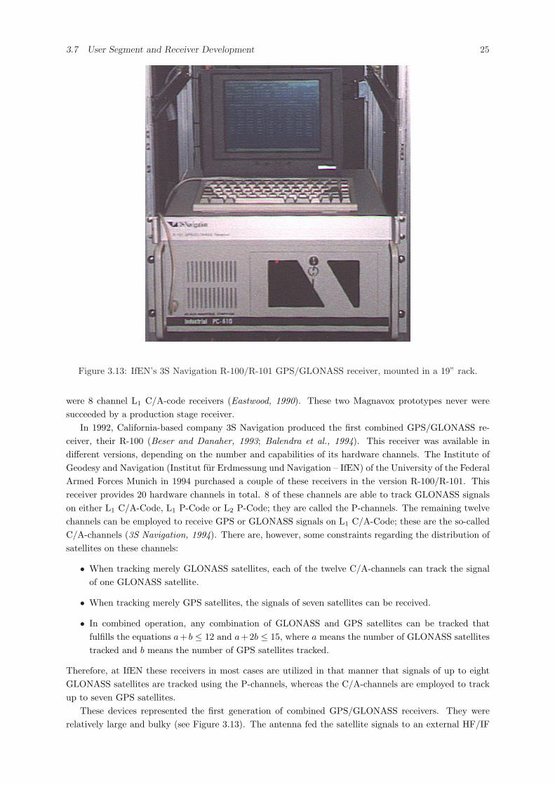
3.7 User Segment and Receiver Development 25
Figure 3.13: IfEN’s 3S Navigation R-100/R-101 GPS/GLONASS receiver, mounted in a 19” rack.
were 8 channel L1 C/A-code receivers (Eastwood, 1990). These two Magnavox prototypes never weresucceeded by a production stage receiver.
In 1992, California-based company 3S Navigation produced the first combined GPS/GLONASS re-ceiver, their R-100 (Beser and Danaher, 1993; Balendra et al., 1994). This receiver was available indifferent versions, depending on the number and capabilities of its hardware channels. The Institute ofGeodesy and Navigation (Institut fur Erdmessung und Navigation – IfEN) of the University of the FederalArmed Forces Munich in 1994 purchased a couple of these receivers in the version R-100/R-101. Thisreceiver provides 20 hardware channels in total. 8 of these channels are able to track GLONASS signalson either L1 C/A-Code, L1 P-Code or L2 P-Code; they are called the P-channels. The remaining twelvechannels can be employed to receive GPS or GLONASS signals on L1 C/A-Code; these are the so-calledC/A-channels (3S Navigation, 1994). There are, however, some constraints regarding the distribution ofsatellites on these channels:
• When tracking merely GLONASS satellites, each of the twelve C/A-channels can track the signalof one GLONASS satellite.
• When tracking merely GPS satellites, the signals of seven satellites can be received.
• In combined operation, any combination of GLONASS and GPS satellites can be tracked thatfulfills the equations a+ b ≤ 12 and a+2b ≤ 15, where a means the number of GLONASS satellitestracked and b means the number of GPS satellites tracked.
Therefore, at IfEN these receivers in most cases are utilized in that manner that signals of up to eightGLONASS satellites are tracked using the P-channels, whereas the C/A-channels are employed to trackup to seven GPS satellites.
These devices represented the first generation of combined GPS/GLONASS receivers. They wererelatively large and bulky (see Figure 3.13). The antenna fed the satellite signals to an external HF/IF
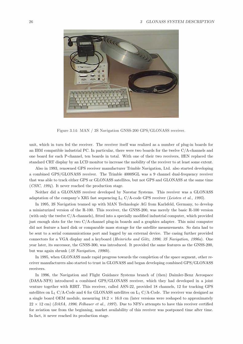
26 3 GLONASS SYSTEM DESCRIPTION
Figure 3.14: MAN / 3S Navigation GNSS-200 GPS/GLONASS receiver.
unit, which in turn fed the receiver. The receiver itself was realized as a number of plug-in boards foran IBM compatible industrial PC. In particular, there were two boards for the twelve C/A-channels andone board for each P-channel, ten boards in total. With one of their two receivers, IfEN replaced thestandard CRT display by an LCD monitor to increase the mobility of the receiver to at least some extent.
Also in 1993, renowned GPS receiver manufacturer Trimble Navigation, Ltd. also started developinga combined GPS/GLONASS receiver. The Trimble 4000SGL was a 9 channel dual-frequency receiverthat was able to track either GPS or GLONASS satellites, but not GPS and GLONASS at the same time(CSIC, 1994). It never reached the production stage.
Neither did a GLONASS receiver developed by Navstar Systems. This receiver was a GLONASSadaptation of the company’s XR5 fast sequencing L1 C/A-code GPS receiver (Leisten et al., 1995).
In 1995, 3S Navigation teamed up with MAN Technologie AG from Karlsfeld, Germany, to developa miniaturized version of the R-100. This receiver, the GNSS-200, was merely the basic R-100 version(with only the twelve C/A-channels), fitted into a specially modified industrial computer, which providedjust enough slots for the two C/A-channel plug-in boards and a graphics adapter. This mini computerdid not feature a hard disk or comparable mass storage for the satellite measurements. So data had tobe sent to a serial communications port and logged by an external device. The casing further providedconnectors for a VGA display and a keyboard (Heinrichs and Gotz, 1996; 3S Navigation, 1996a). Oneyear later, its successor, the GNSS-300, was introduced. It provided the same features as the GNSS-200,but was again shrunk (3S Navigation, 1996b).
In 1995, when GLONASS made rapid progress towards the completion of the space segment, other re-ceiver manufacturers also started to trust in GLONASS and began developing combined GPS/GLONASSreceivers.
In 1996, the Navigation and Flight Guidance Systems branch of (then) Daimler-Benz Aerospace(DASA-NFS) introduced a combined GPS/GLONASS receiver, which they had developed in a jointventure together with RIRT. This receiver, called ASN-22, provided 18 channels, 12 for tracking GPSsatellites on L1 C/A-Code and 6 for GLONASS satellites on L1 C/A-Code. The receiver was designed asa single board OEM module, measuring 18.2 × 16.0 cm (later versions were reshaped to approximately22 × 12 cm) (DASA, 1996; Felhauer et al., 1997). Due to NFS’s attempts to have this receiver certifiedfor aviation use from the beginning, market availability of this receiver was postponed time after time.In fact, it never reached its production stage.
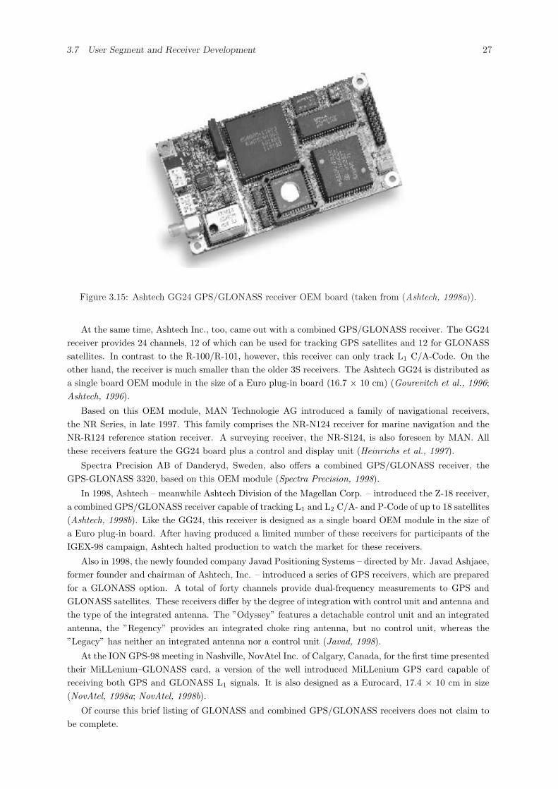
3.7 User Segment and Receiver Development 27
Figure 3.15: Ashtech GG24 GPS/GLONASS receiver OEM board (taken from (Ashtech, 1998a)).
At the same time, Ashtech Inc., too, came out with a combined GPS/GLONASS receiver. The GG24receiver provides 24 channels, 12 of which can be used for tracking GPS satellites and 12 for GLONASSsatellites. In contrast to the R-100/R-101, however, this receiver can only track L1 C/A-Code. On theother hand, the receiver is much smaller than the older 3S receivers. The Ashtech GG24 is distributed asa single board OEM module in the size of a Euro plug-in board (16.7 × 10 cm) (Gourevitch et al., 1996;Ashtech, 1996).
Based on this OEM module, MAN Technologie AG introduced a family of navigational receivers,the NR Series, in late 1997. This family comprises the NR-N124 receiver for marine navigation and theNR-R124 reference station receiver. A surveying receiver, the NR-S124, is also foreseen by MAN. Allthese receivers feature the GG24 board plus a control and display unit (Heinrichs et al., 1997).
Spectra Precision AB of Danderyd, Sweden, also offers a combined GPS/GLONASS receiver, theGPS-GLONASS 3320, based on this OEM module (Spectra Precision, 1998).
In 1998, Ashtech – meanwhile Ashtech Division of the Magellan Corp. – introduced the Z-18 receiver,a combined GPS/GLONASS receiver capable of tracking L1 and L2 C/A- and P-Code of up to 18 satellites(Ashtech, 1998b). Like the GG24, this receiver is designed as a single board OEM module in the size ofa Euro plug-in board. After having produced a limited number of these receivers for participants of theIGEX-98 campaign, Ashtech halted production to watch the market for these receivers.
Also in 1998, the newly founded company Javad Positioning Systems – directed by Mr. Javad Ashjaee,former founder and chairman of Ashtech, Inc. – introduced a series of GPS receivers, which are preparedfor a GLONASS option. A total of forty channels provide dual-frequency measurements to GPS andGLONASS satellites. These receivers differ by the degree of integration with control unit and antenna andthe type of the integrated antenna. The ”Odyssey” features a detachable control unit and an integratedantenna, the ”Regency” provides an integrated choke ring antenna, but no control unit, whereas the”Legacy” has neither an integrated antenna nor a control unit (Javad, 1998).
At the ION GPS-98 meeting in Nashville, NovAtel Inc. of Calgary, Canada, for the first time presentedtheir MiLLenium–GLONASS card, a version of the well introduced MiLLenium GPS card capable ofreceiving both GPS and GLONASS L1 signals. It is also designed as a Eurocard, 17.4 × 10 cm in size(NovAtel, 1998a; NovAtel, 1998b).
Of course this brief listing of GLONASS and combined GPS/GLONASS receivers does not claim tobe complete.
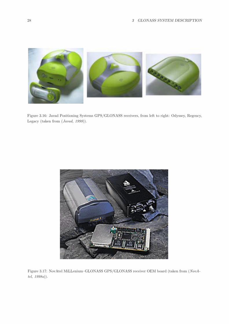
28 3 GLONASS SYSTEM DESCRIPTION
Figure 3.16: Javad Positioning Systems GPS/GLONASS receivers, from left to right: Odyssey, Regency,Legacy (taken from (Javad, 1998)).
Figure 3.17: NovAtel MiLLenium–GLONASS GPS/GLONASS receiver OEM board (taken from (NovA-tel, 1998a)).
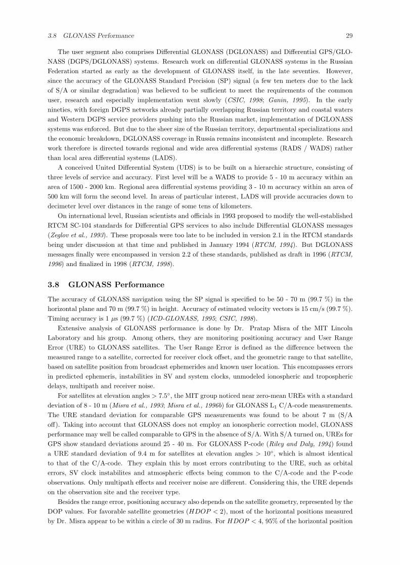
3.8 GLONASS Performance 29
The user segment also comprises Differential GLONASS (DGLONASS) and Differential GPS/GLO-NASS (DGPS/DGLONASS) systems. Research work on differential GLONASS systems in the RussianFederation started as early as the development of GLONASS itself, in the late seventies. However,since the accuracy of the GLONASS Standard Precision (SP) signal (a few ten meters due to the lackof S/A or similar degradation) was believed to be sufficient to meet the requirements of the commonuser, research and especially implementation went slowly (CSIC, 1998; Ganin, 1995). In the earlynineties, with foreign DGPS networks already partially overlapping Russian territory and coastal watersand Western DGPS service providers pushing into the Russian market, implementation of DGLONASSsystems was enforced. But due to the sheer size of the Russian territory, departmental specializations andthe economic breakdown, DGLONASS coverage in Russia remains inconsistent and incomplete. Researchwork therefore is directed towards regional and wide area differential systems (RADS / WADS) ratherthan local area differential systems (LADS).
A conceived United Differential System (UDS) is to be built on a hierarchic structure, consisting ofthree levels of service and accuracy. First level will be a WADS to provide 5 - 10 m accuracy within anarea of 1500 - 2000 km. Regional area differential systems providing 3 - 10 m accuracy within an area of500 km will form the second level. In areas of particular interest, LADS will provide accuracies down todecimeter level over distances in the range of some tens of kilometers.
On international level, Russian scientists and officials in 1993 proposed to modify the well-establishedRTCM SC-104 standards for Differential GPS services to also include Differential GLONASS messages(Zeglov et al., 1993). These proposals were too late to be included in version 2.1 in the RTCM standardsbeing under discussion at that time and published in January 1994 (RTCM, 1994). But DGLONASSmessages finally were encompassed in version 2.2 of these standards, published as draft in 1996 (RTCM,1996) and finalized in 1998 (RTCM, 1998).
3.8 GLONASS Performance
The accuracy of GLONASS navigation using the SP signal is specified to be 50 - 70 m (99.7 %) in thehorizontal plane and 70 m (99.7 %) in height. Accuracy of estimated velocity vectors is 15 cm/s (99.7 %).Timing accuracy is 1 µs (99.7 %) (ICD-GLONASS, 1995; CSIC, 1998).
Extensive analysis of GLONASS performance is done by Dr. Pratap Misra of the MIT LincolnLaboratory and his group. Among others, they are monitoring positioning accuracy and User RangeError (URE) to GLONASS satellites. The User Range Error is defined as the difference between themeasured range to a satellite, corrected for receiver clock offset, and the geometric range to that satellite,based on satellite position from broadcast ephemerides and known user location. This encompasses errorsin predicted ephemeris, instabilities in SV and system clocks, unmodeled ionospheric and troposphericdelays, multipath and receiver noise.
For satellites at elevation angles > 7.5◦, the MIT group noticed near zero-mean UREs with a standarddeviation of 8 - 10 m (Misra et al., 1993; Misra et al., 1996b) for GLONASS L1 C/A-code measurements.The URE standard deviation for comparable GPS measurements was found to be about 7 m (S/Aoff). Taking into account that GLONASS does not employ an ionospheric correction model, GLONASSperformance may well be called comparable to GPS in the absence of S/A. With S/A turned on, UREs forGPS show standard deviations around 25 - 40 m. For GLONASS P-code (Riley and Daly, 1994) founda URE standard deviation of 9.4 m for satellites at elevation angles > 10◦, which is almost identicalto that of the C/A-code. They explain this by most errors contributing to the URE, such as orbitalerrors, SV clock instabilites and atmospheric effects being common to the C/A-code and the P-codeobservations. Only multipath effects and receiver noise are different. Considering this, the URE dependson the observation site and the receiver type.
Besides the range error, positioning accuracy also depends on the satellite geometry, represented by theDOP values. For favorable satellite geometries (HDOP < 2), most of the horizontal positions measuredby Dr. Misra appear to be within a circle of 30 m radius. For HDOP < 4, 95% of the horizontal position
30 3 GLONASS SYSTEM DESCRIPTION
estimates lie within a circle of 30 m radius (Misra et al., 1993). With a complete GLONASS constellation,93% of the users are expected to have an HDOP < 2. Therefore it can be said that GLONASS shouldeasily meet its specifications. For satellite geometries with an HDOP < 5, (Riley and Daly, 1994) foundthe horizontal positioning error using GLONASS P-code to be approximately 40 m (2drms).
On the other hand, (Misra et al., 1993) also revealed some glitches in system operations and upkeep.Due to the ground monitoring and upload stations being distributed over the territory of the formerUSSR only, satellite failures may go undetected for some hours, until that satellite again reaches thevisibility area of the monitoring stations. Even more time will pass, until updated almanac data couldbe uploaded to all satellites.
The fact that GLONASS time is tightly coupled to UTC and thus introduces leap seconds wheneverUTC introduces leap seconds also is a source of potential system anomalies. (Misra et al., 1993) reportsUser Range Errors with magnitudes of some hundred meters occurring between 0:00:00h and around1:00:00h on July 1, 1992, when a leap second was introduced. Later introductions of leap seconds onJune 30, 1993, and December 31, 1995, caused GLONASS to trip for about three minutes each (Misraet al., 1996b). According to the ICD (ICD-GLONASS, 1995), the two-second lines of the GLONASSnavigation message are to begin at an even number of seconds within the day in the satellite time frame.By introducing a leap second, the number of seconds within a day suddenly becomes uneven, with twosucceeding even second epochs. Half-way through the first line of the first frame of a superframe, thisline has to be aborted and restarted. Obviously this process, along with the re-adjustment of the satelliteclocks, causes problems to the data generation on-board the satellites.
When introducing a leap second in the night of June 30 to July 1, 1997, the whole GLONASS systemwent down for one day. However, as will be explained later, on that occasion not only a leap second wasintroduced, but also the GLONASS time frame was corrected to be closer to UTC. The system beingdown that day was announced eleven days in advance (CSIC, 1997). But shutting down the system foran entire day or only for a few minutes is not suitable to support the possible use of GLONASS as a solemeans of navigation.
31
4 Time Systems
GPS and GLONASS both use their own time scales, which, in addition, are connected to differentrealizations of UTC. Therefore, GPS time and GLONASS time cannot easily be transformed from onetime scale into the other.
In combined GPS/GLONASS data processing the differences between these time scales must beaccounted for. Otherwise, systematic errors are introduced that will affect the combined positioningsolution.
4.1 GLONASS Time
GLONASS system time is maintained by the GLONASS Central Synchronizer by means of a set ofhydrogen masers (Gouzhva et al., 1995). It is closely coupled to UTC, but with a constant offset of threehours (corresponding to the offset of Moscow time to Greenwich time). Therefore, GLONASS system timealso considers leap seconds. Further differences between GLONASS time and UTC arise from the keepingof the time scales by two different master clocks. These differences are in the order of microseconds. InOctober / November 1996, for example, this difference was around (tUTC − tGLONASS) mod 1 h = −25 µs(RNTFS, 1996a).
The GLONASS user is informed about the difference to UTC as maintained by the National Etalonof Time and Frequency in Moscow (UTCSU). This information is obtained from the UTC parameter τc
in frame 5 of the GLONASS ephemerides message (ICD-GLONASS, 1995).UTC then can be computed from GLONASS time according to the simple relation
tUTC = tGLONASS + τc − 3 h (4.1.1)
The accuracy of this computed tUTC is specified to be less than 1 µs (ICD-GLONASS, 1995).On-board the GLONASS satellites, Cesium frequency standards are used. These clocks are specified
to have a frequency instability of less than 5× 10⁻¹³ (the satellites launched in 1995 have cesium clockswith frequency instabilities less than 1×10⁻¹³) (Gouzhva et al., 1995). With time and frequency uploadsto the satellite twice a day, this stability provides an accuracy of satellite time synchronization to systemtime of about 15 ns (1 σ). Accuracy of the uploaded corrections is specified to be less than 35 ns (1 σ).
4.2 GPS Time
GPS system time is maintained by the GPS Master Control Station. It was started on January 6, 1980.Since it is a uniform time scale, it differs from UTC by the leap seconds introduced into the latter timescale. Currently (February 2000) this difference is 13 seconds. In addition to the leap seconds, furtherdifferences between GPS system time and UTC arise from the fact that GPS system time and UTC arekept by different master clocks. These additional differences are in the order of nanoseconds. In fact,GPS operators usually keep GPS system time to within 100 ns of UTC as maintained by the US NavalObservatory (UTCUSNO). In December 1994, however, due to a malfunction, GPS system time madean excursion of about 270 ns from UTC for a period of about two weeks (Lewandowski et al., 1997) .
The GPS user is informed about the difference to UTCUSNO. This information is obtained fromthe UTC parameters in page 18 of subframe 4 of the GPS ephemerides message. This set of parametersconsists of the following values (ICD-GPS, 1991):
WNt Reference time of UTC parameters (week number)tot Reference time of UTC parameters (s into week)∆tLS Number of leap secondsA0, A1 Polynomial coefficientsWNLSF Time of next scheduled change of leap seconds (week number)DN Number of day in WNLSF , at the end of which leap seconds will change∆tLSF Future value of leap seconds
32 4 TIME SYSTEMS
For the computation of UTC from GPS time, three cases must be distinguished:
1. The time given by WNLSF and DN is not in the past and the present time is not in the interval[DN + 3/4, DN + 5/4].
In this case UTC computes to:
tUTC = (tGPS −∆tUTC) mod 86400 (4.2.1)
with
∆tUTC = ∆tLS + A0 + A1 (tGPS − tot + (WN −WNt) · 604800) (4.2.2)
2. The present time is in the interval [DN + 3/4, DN + 5/4].
In this case UTC computes to:
tUTC = W mod (86400 + ∆tLSF −∆tLS) (4.2.3)
with
W = (tGPS −∆tUTC − 43200) mod 86400 + 43200 (4.2.4)
and ∆tUTC as given in Eq. (4.2.2).
3. The time given by WNLSF and DN is in the past.
In this case UTC is computed analogously to case 1, but ∆tLSF has to be substituted for ∆tLS inEq. (4.2.2).
In these equations, tGPS is always given in seconds into the week, whereas tUTC is given in seconds intoday. Therefore the modulo operations are performed. The accuracy of this computed tUTC is specifiedto be less than 90 ns (1 σ) (ICD-GPS, 1991).
4.3 UTC, UTCUSNO, UTCSU and GLONASS System Time
UTC is obtained from a combination of data from about 230 atomic clocks in 60 laboratories world-wide(BIPM, 1995). 47 timing centers are maintaining a local UTC. UTCUSNO and UTCSU are two of theselocal UTCs. UTCUSNO is kept by an ensemble of cesium standards and hydrogen masers. Its differenceto UTC is in the order of some ns. It generally remains within 20 ns. UTCSU is kept by an ensemble ofhydrogen masers and is regarded as one of the most stable atomic time scales in the world (Lewandowskiet al., 1996). Its difference to UTC is in the order of some µs. Hence the difference between UTCUSNOand UTCSU also is in the order of some µs. In October / November 1996, for example, this differencewas around UTCSU−UTC = 7.95 µs (RNTFS, 1996a). The difference UTCSU− tGPS was around 8 µs.
Following Recommendation S4 (1996) of the Comite Consultatif pour la Definition de la Seconde(CCDS), which recommends that the reference times of satellite navigation systems with global cov-erage be synchronized as closely as possible to UTC (CCDS, 1996), on November 27, 1996, 0h 0m 0sUT, UTCSU was corrected by 9 µs, yielding the difference UTCSU old − UTCSU new = 9 µs (MMC,1996). Thus, after November 27, 1996 the difference UTCSU − UTC was around −1 µs, the differ-ence UTCSU − tGPS was around −0.9 µs. The difference between UTCSU and GLONASS system timebecame (tUTC − tGLONASS) mod 1 h = −35 µs (RNTFS, 1996b).
After this change, UTCSU slowly drifted towards UTC, and in May 1997 the offsets UTCSU −UTC
and UTCSU − tGPS both were approximately −0.7 µs (RNTFS, 1997).In a next step to comply with CCDS Recommendation S4 (1996), on January 10, 1997, the fre-
quency of the GLONASS Central Synchronizer clocks was slightly changed, bringing it closer to that
4.4 Resolving the Time Reference Difference 33
of UTCSU and thus stabilizing the difference between GLONASS system time and UTC at around(tUTC − tGLONASS) mod 1 h = −35.9 µs. Subsequently, at midnight of July 1, 1997, GLONASS systemtime received a time step of approximately 35.3 µs (Langley, 1997). This moved both UTCSU and GLO-NASS system time to within a few hundred nanoseconds of UTC (Lewandowski and Azoubib, 1998). Dateand time for this operation were set to coincide with a leap second step in UTC. Further adjustments ofthese two time scales (UTCSU and GLONASS system time) are expected.
Since the data from the local timing centers are not compared and combined to UTC in real-time, thedifference between UTCUSNO and UTCSU and therefore the difference between GPS and GLONASSsystem time neither is directly (a-priori) available in real-time. This is the crucial problem to be solvedwhen combining GPS and GLONASS data in navigation or in other near real-time operation.
4.4 Resolving the Time Reference Difference
To determine this difference in the time reference systems, a number of procedures are possible. Aselection of these procedures will be described and discussed in the following.
4.4.1 Introducing a Second Receiver Clock Offset
In this method, different receiver clock offsets are introduced with respect to GPS and GLONASS systemtime. These two clock offsets are instantaneously determined at each observation epoch together withthe three unknowns of the receiver position.
Starting with a simplified non-linear observation equation (for the complete observation equations seeChapter 8) for a pseudorange observation to a satellite S of an arbitrary system (GPS or GLONASS) atan observer R,
PRSR = %S
R + c · δtR − c · δtS (4.4.1)
and by introducing a Taylor series expansion around an approximate position P0, we obtain the linearizedequation
PRSR = %S
0 +x0 − xS
%S0
· (xR − x0) +y0 − yS
%S0
· (yR − y0) +z0 − zS
%S0
· (zR − z0) + c · δtR − c · δtS(4.4.2)
with x0, y0, z0 being the coordinates of the approximate position and
%S0 =
√(x0 − xS)2 + (y0 − yS)2 + (z0 − zS)2
being the geometric distance between the approximate position and the satellite position.With the receiver clock error δtR = tR − tSys (tSys being the GPS or GLONASS system time tGPS
or tGLONASS , respectively) as one of the unknowns being a function of the system time tSys, it becomesclear that in mixed GPS/GLONASS processing two receiver clock errors will have to be introduced, onefor the receiver clock offset with respect to GPS time and one for the receiver clock offset with respectto GLONASS time. We then obtain two different observation equations for a GPS satellite i and aGLONASS satellite j:
PRGPS iR = %GPS i
0 +x0 − xGPS i
%GPS i0
· (xR − x0) +y0 − yGPS i
%GPS i0
· (yR − y0) + (4.4.3)
z0 − zGPS i
%GPS i0
· (zR − z0) + c · δtR,GPS − c · δtGPS i
PRGLO jR = %GLO j
0 +x0 − xGLO j
%GLO j0
· (xR − x0) +y0 − yGLO j
%GLO j0
· (yR − y0) + (4.4.4)
z0 − zGLO j
%GLO j0
· (zR − z0) + c · δtR,GLONASS − c · δtGLO j
34 4 TIME SYSTEMS
Due to the additional unknown, an additional (fifth) observation is necessary to obtain a positioningsolution. Since the combined use of GPS and GLONASS approximately doubles the number of obser-vations with respect to GLONASS or GPS alone (at least for the full GLONASS constellation), thissacrificing of one observation can easily be accepted. Generally, as long as at least two satellites ofone system (GPS or GLONASS) are added to observations of the other system, this sacrificing of onemeasurement is acceptable.
Having a sufficient number of observations to both GPS and GLONASS satellites, the set of observa-tion equations can be written in matrix notation:
~l = A · ~x (4.4.5)
with
~l =
PRiR − %i
0 + c · δtiPRj
R − %j0 + c · δtj
PRkR − %k
0 + c · δtk...
(4.4.6)
the vector of the known values,
A =
x0 − xi
%i0
y0 − yi
%i0
z0 − zi
%i0
1 0
x0 − xj
%j0
y0 − yj
%j0
z0 − zj
%j0
0 1
x0 − xk
%k0
y0 − yk
%k0
z0 − zk
%k0
1 0
......
......
...
(4.4.7)
the design matrix (k being a GPS satellite), and
~x =
(xR − x0)(yR − y0)(zR − z0)c · δtR,GPS
c · δtR,GLONASS
=
(xR − x0)(yR − y0)(zR − z0)
c · (tR − tGPS)c · (tR − tGLONASS)
(4.4.8)
the vector of the unknowns.This system of equations can then be solved using the conventional methods, e.g. a least squares
adjustment or Kalman filtering.It should be noted that a solution of these equations is only possible, if indeed there are observations
to satellites of both GPS and GLONASS. For observations to GPS or GLONASS satellites only, however,only one receiver clock offset is required. Furthermore, if all but one observed satellites are from onesystem, with only one satellite from the second system, this additional observation contributes only tothe second receiver clock offset, but does not influence the computed position.
4.4.2 Introducing the Difference in System Time Scales
Starting with the pair of Eqs. (4.4.3) and (4.4.4), we can rewrite the receiver clock offset to GLONASSsystem time:
δtR,GLONASS = tR − tGLONASS = tR − tGPS + tGPS − tGLONASS (4.4.9)
Eq. (4.4.4) then transforms to
PRGLO jR = %GLO j
0 +x0 − xGLO j
%GLO j0
· (xR − x0) +y0 − yGLO j
%GLO j0
· (yR − y0) + (4.4.10)
z0 − zGLO j
%GLO j0
· (zR − z0) + c · δtR,GPS + c · (tGPS − tGLONASS)− c · δtGLO j
4.4 Resolving the Time Reference Difference 35
Together with Eq. (4.4.3) we can now set up a new system of observation equations in matrix notation,identical to Eq. (4.4.5), but with modified design matrix and vector of unknowns:
A =
x0 − xi
%i0
y0 − yi
%i0
z0 − zi
%i0
1 0
x0 − xj
%j0
y0 − yj
%j0
z0 − zj
%j0
1 1
x0 − xk
%k0
y0−yk
%k0
z0 − zk
%k0
1 0
......
......
...
(4.4.11)
~x =
(xR − x0)(yR − y0)(zR − z0)
c · (tR − tGPS)c · (tGPS − tGLONASS)
(4.4.12)
This method principally is equivalent to the one described in Section 4.4.1 (Eqs. (4.4.6) - (4.4.8)), butit is more elegant. The additional unknown (tGPS − tGLONASS) as the difference in system time scales isnow independent of the receiver. Thus, when forming differences of the same kind between two receivers(receiver-receiver single differences), this unknown cancels out.
Similar to the case of two separate receiver clock offsets, a solution of these equations is only possible,if indeed there are observations to satellites of both GPS and GLONASS. For observations to GPS orGLONASS satellites only, however, only the receiver clock offset is required. Furthermore, if all but oneobserved satellites are from one system, with only one satellite from the second system, this additionalobservation contributes only to the difference in system time frames, but does not influence the computedposition.
4.4.3 Application of A-priori Known Time Offsets
In this method, the difference in system time between GPS and GLONASS (or the difference betweenUTCUSNO and UTCSU, respectively) is considered to be known a-priori from some external knowledge.This is a very effective method in the sense of one unknown being eliminated.
Having a-priori knowledge of the difference between GPS and GLONASS time (tGPS − tGLONASS),the respective term in Eq. (4.4.10) is shifted to the left-hand side of the equation, when writing thematrix notation according to Eq. (4.4.5). The result is a system of observation equations with modifiedvectors and design matrix:
~l = A · ~x (4.4.13)
with
~l =
PRiR − %i
0 + c · δtiPRj
R − %j0 + c · δtj − c · (tGPS − tGLONASS)
PRkR − %k
0 + c · δtk...
(4.4.14)
A =
x0 − xi
%i0
y0 − yi
%i0
z0 − zi
%i0
1
x0 − xj
%j0
y0 − yj
%j0
z0 − zj
%j0
1
x0 − xk
%k0
y0 − yk
%k0
z0 − zk
%k0
1
......
......
(4.4.15)
36 4 TIME SYSTEMS
~x =
(xR − x0)(yR − y0)(zR − z0)c · δtR,GPS
=
(xR − x0)(yR − y0)(zR − z0)
c · (tR − tGPS)
(4.4.16)
As stated above, however, the exact difference between UTCUSNO and UTCSU and therefore thedifference between GPS and GLONASS system times definitely is not available in real-time as externalknowledge. Thus, this method is only applicable in a post-mission analysis software for geodetic ap-plications, but not in real-time GPS/GLONASS navigation or other (near) real-time applications. Inthe latter case, a time series of these differences could be used to extrapolate the instantaneous timedifference, with all the uncertainties that come along with extrapolations.
4.4.4 Dissemination of Difference in Time Reference
The Russian Military Space Forces as the operator of the GLONASS system are planning to includethe time difference between GLONASS system time and GPS system time in the navigation messageof the next generation of GLONASS satellites, the so-called GLONASS-M spacecraft (Ivanov et al.,1995; Kazantsev, 1995). In principle, this will be equivalent to the use of a-priori known time offsets, asdescribed in Section 4.4.3, but it will drop the need for determining this time offset during processing.The problem of possible loss of accuracy in the extrapolated time offsets, however, will remain. It willonly shift from the user to the GLONASS Control Center. But given their experience in monitoring theGLONASS system clock and forecasting clock offsets, the broadcast time difference between GLONASStime and GPS time can be expected to be sufficiently accurate.
As stated above, the dissemination of this time difference in the broadcast navigation message isplanned for the GLONASS-M satellites. According to the latest version of the GLONASS ICD (ICD-GLONASS, 1998), GLONASS-M satellites will broadcast a τGPS data word. This will specify the frac-tional part (as expressed in seconds) of the difference between GPS and GLONASS system time scales.The difference between these two time scales can then be obtained as
tGPS − tGLONASS = ∆tLS + τGPS (4.4.17)
with ∆tLS being the number of leap seconds between GPS time and UTC. This value is broadcast in theGPS navigation message.
The first launch of a GLONASS-M satellite originally was scheduled for 1996, but was delayed dueto the economic problems in Russia. Up to now (February 2000), not a single GLONASS-M satellite hasin fact been launched. And it seems uncertain, if the GLONASS-M program will ever be realized at all.Thus, for the time being one of the methods described in the previous sections will have to be applied.
4.5 Conclusions
A number of possible methods to resolve the difference in reference time between GPS and GLONASShave been described in the previous sections. For a decision, which of them is best to be implemented incombined GPS/GLONASS data processing, two cases must be considered:
• There is no GLONASS-M satellite among the tracked satellites.
In this case, the time difference between GPS time and GLONASS system time is not known atprocessing time. Therefore, a measure of the difference in reference time must be determined asan additional unknown during processing. The most promising way to do so is to estimate thetime difference between GPS time and GLONASS time itself rather than introducing a separatereceiver clock error with respect to GLONASS time. Thus, the five unknowns to be solved for arethe three coordinates of the receiver position, the receiver clock offset to GPS system time plus thetime difference between GPS time and GLONASS time. The implementation of this method wasdescribed in Section 4.4.2.
4.5 Conclusions 37
• There is at least one GLONASS-M satellite among the tracked satellites.
In this case, the time difference between GPS time and GLONASS system time is disseminatedas part of the satellite navigation message and can be considered to be known. This reduces thenumber of unknowns to be determined during processing to four, namely the three coordinatesof the receiver position plus the receiver clock offset to GPS or GLONASS system time. Theseare the same unknowns that are already solved for in GPS or GLONASS only processing. Theimplementation of this method was described in Section 4.4.4.
However, as long as no GLONASS-M satellites have been launched, considering this case is merelyof academic interest.
Even in the latter case, an additional determination of the difference between GPS time and GLONASStime still could be performed, e.g. for purposes of integrity monitoring in safety-critical applications (airnavigation) or for enhancing the accuracy of the broadcast value of this difference in high precisionapplications.

38 4 TIME SYSTEMS
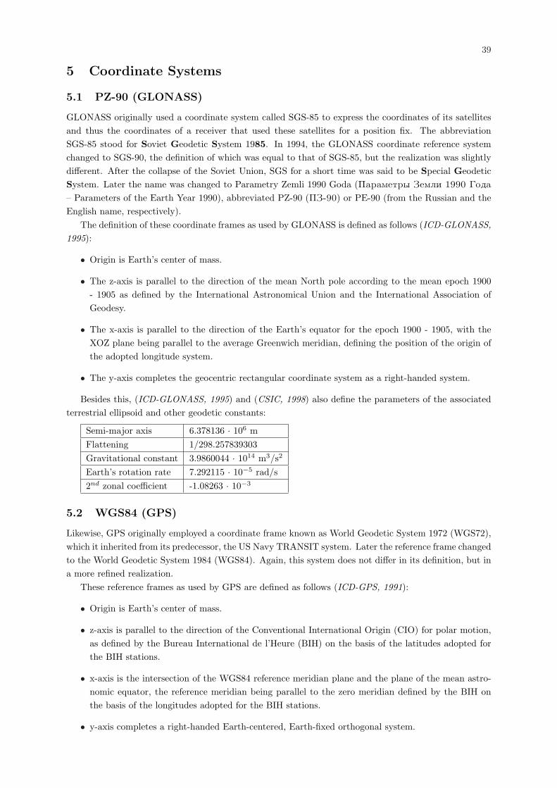
39
5 Coordinate Systems
5.1 PZ-90 (GLONASS)
GLONASS originally used a coordinate system called SGS-85 to express the coordinates of its satellitesand thus the coordinates of a receiver that used these satellites for a position fix. The abbreviationSGS-85 stood for Soviet Geodetic System 1985. In 1994, the GLONASS coordinate reference systemchanged to SGS-90, the definition of which was equal to that of SGS-85, but the realization was slightlydifferent. After the collapse of the Soviet Union, SGS for a short time was said to be Special GeodeticSystem. Later the name was changed to Parametry Zemli 1990 Goda (Parametry Zemli 1990 Goda– Parameters of the Earth Year 1990), abbreviated PZ-90 (PZ-90) or PE-90 (from the Russian and theEnglish name, respectively).
The definition of these coordinate frames as used by GLONASS is defined as follows (ICD-GLONASS,1995):
• Origin is Earth’s center of mass.
• The z-axis is parallel to the direction of the mean North pole according to the mean epoch 1900- 1905 as defined by the International Astronomical Union and the International Association ofGeodesy.
• The x-axis is parallel to the direction of the Earth’s equator for the epoch 1900 - 1905, with theXOZ plane being parallel to the average Greenwich meridian, defining the position of the origin ofthe adopted longitude system.
• The y-axis completes the geocentric rectangular coordinate system as a right-handed system.
Besides this, (ICD-GLONASS, 1995) and (CSIC, 1998) also define the parameters of the associatedterrestrial ellipsoid and other geodetic constants:
Semi-major axis 6.378136 · 106 mFlattening 1/298.257839303Gravitational constant 3.9860044 · 1014 m3/s2
Earth’s rotation rate 7.292115 · 10−5 rad/s2nd zonal coefficient -1.08263 · 10−3
5.2 WGS84 (GPS)
Likewise, GPS originally employed a coordinate frame known as World Geodetic System 1972 (WGS72),which it inherited from its predecessor, the US Navy TRANSIT system. Later the reference frame changedto the World Geodetic System 1984 (WGS84). Again, this system does not differ in its definition, but ina more refined realization.
These reference frames as used by GPS are defined as follows (ICD-GPS, 1991):
• Origin is Earth’s center of mass.
• z-axis is parallel to the direction of the Conventional International Origin (CIO) for polar motion,as defined by the Bureau International de l’Heure (BIH) on the basis of the latitudes adopted forthe BIH stations.
• x-axis is the intersection of the WGS84 reference meridian plane and the plane of the mean astro-nomic equator, the reference meridian being parallel to the zero meridian defined by the BIH onthe basis of the longitudes adopted for the BIH stations.
• y-axis completes a right-handed Earth-centered, Earth-fixed orthogonal system.
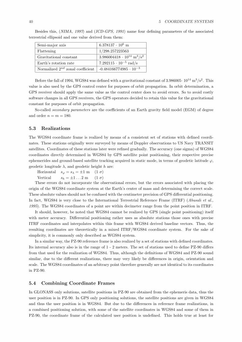
40 5 COORDINATE SYSTEMS
Besides this, (NIMA, 1997) and (ICD-GPS, 1991) name four defining parameters of the associatedterrestrial ellipsoid and one value derived from them:
Semi-major axis 6.378137 · 106 mFlattening 1/298.257223563Gravitational constant 3.986004418 · 1014 m3/s2
Earth’s rotation rate 7.292115 · 10−5 rad/sNormalized 2nd zonal coefficient -0.484166774985 · 10−3
Before the fall of 1994, WGS84 was defined with a gravitational constant of 3.986005· 1014 m3/s2. Thisvalue is also used by the GPS control center for purposes of orbit propagation. In orbit determination, aGPS receiver should apply the same value as the control center does to avoid errors. So to avoid costlysoftware changes in all GPS receivers, the GPS operators decided to retain this value for the gravitationalconstant for purposes of orbit propagation.
So-called secondary parameters are the coefficients of an Earth gravity field model (EGM) of degreeand order n = m = 180.
5.3 Realizations
The WGS84 coordinate frame is realized by means of a consistent set of stations with defined coordi-nates. These stations originally were surveyed by means of Doppler observations to US Navy TRANSITsatellites. Coordinates of these stations later were refined gradually. The accuracy (one sigma) of WGS84coordinates directly determined in WGS84 by GPS satellite point positioning, their respective preciseephemerides and ground-based satellite tracking acquired in static mode, in terms of geodetic latitude ϕ,geodetic longitude λ, and geodetic height h are:
Horizontal sϕ = sλ = ±1 m (1 σ)Vertical sh = ±1 . . . 2 m (1 σ)
These errors do not incorporate the observational errors, but the errors associated with placing theorigin of the WGS84 coordinate system at the Earth’s center of mass and determining the correct scale.These absolute values should not be confused with the centimeter precision of GPS differential positioning.In fact, WGS84 is very close to the International Terrestrial Reference Frame (ITRF) (Abusali et al.,1995). The WGS84 coordinates of a point are within decimeter range from the point position in ITRF.
It should, however, be noted that WGS84 cannot be realized by GPS (single point positioning) itselfwith meter accuracy. Differential positioning rather uses as absolute stations those ones with preciseITRF coordinates and interpolates within this frame with WGS84 derived baseline vectors. Thus, theresulting coordinates are theoretically in a mixed ITRF/WGS84 coordinate system. For the sake ofsimplicity, it is commonly only described as WGS84 system.
In a similar way, the PZ-90 reference frame is also realized by a set of stations with defined coordinates.Its internal accuracy also is in the range of 1 - 2 meters. The set of stations used to define PZ-90 differsfrom that used for the realization of WGS84. Thus, although the definitions of WGS84 and PZ-90 soundsimilar, due to the different realizations, there may very likely be differences in origin, orientation andscale. The WGS84 coordinates of an arbitrary point therefore generally are not identical to its coordinatesin PZ-90.
5.4 Combining Coordinate Frames
In GLONASS only solutions, satellite positions in PZ-90 are obtained from the ephemeris data, thus theuser position is in PZ-90. In GPS only positioning solutions, the satellite positions are given in WGS84and thus the user position is in WGS84. But due to the differences in reference frame realizations, ina combined positioning solution, with some of the satellite coordinates in WGS84 and some of them inPZ-90, the coordinate frame of the calculated user position is undefined. This holds true at least for
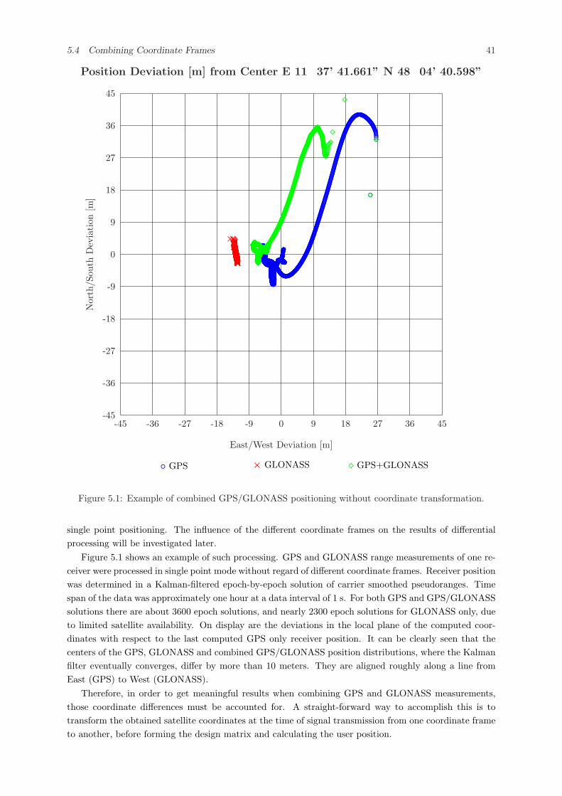
5.4 Combining Coordinate Frames 41
Position Deviation [m] from Center E 11� 37’ 41.661” N 48� 04’ 40.598”
◦ GPS × GLONASS ¦ GPS+GLONASS
East/West Deviation [m]
-45 -36 -27 -18 -9 0 9 18 27 36 45
Nor
th/S
outh
Dev
iati
on[m
]
-45
-36
-27
-18
-9
0
9
18
27
36
45
◦
◦◦◦◦◦◦◦◦◦◦◦◦◦◦◦◦◦◦◦◦◦◦◦◦
◦◦◦◦◦◦◦◦◦◦◦◦◦◦◦◦◦◦◦◦◦◦◦◦◦◦◦◦◦◦◦◦◦◦◦◦◦◦◦◦◦◦◦◦◦◦◦◦◦◦◦◦◦◦◦◦◦◦◦◦◦◦◦◦◦◦◦◦◦◦◦◦◦◦◦◦◦◦◦◦◦◦◦◦◦◦◦◦◦◦◦◦◦◦◦◦◦◦◦◦◦◦◦◦◦◦◦◦◦◦◦◦◦◦◦◦◦◦◦◦◦◦◦◦◦◦◦◦◦◦◦◦◦◦◦◦◦◦◦◦◦◦◦◦◦◦◦◦◦◦◦◦◦◦◦◦◦◦◦◦◦◦◦◦◦◦◦◦◦◦◦◦◦◦◦◦◦◦◦◦◦◦◦◦◦◦◦◦◦◦◦◦◦◦◦◦◦◦◦◦◦◦◦◦◦◦◦◦◦◦◦◦◦◦◦◦◦◦◦◦◦◦◦◦◦◦◦◦◦◦◦◦◦◦◦◦◦◦◦◦◦◦◦◦◦◦◦◦◦◦◦◦◦◦◦◦◦◦◦◦◦◦◦◦◦◦◦◦◦◦◦◦◦◦◦◦◦◦◦◦◦◦◦◦◦◦◦◦◦◦◦◦◦◦◦◦◦◦◦◦◦◦◦◦◦◦◦◦◦◦◦◦◦◦◦◦◦◦◦◦◦◦◦◦◦◦◦◦◦◦◦◦◦◦◦◦◦◦◦◦◦◦◦◦◦◦◦◦◦◦◦◦◦◦◦◦◦◦◦◦◦◦◦◦◦◦◦◦◦◦◦◦◦◦◦◦◦◦◦◦◦◦◦◦◦◦◦◦◦◦◦◦◦◦◦◦◦◦◦◦◦◦◦◦◦◦◦◦◦◦◦◦◦◦◦◦◦◦◦◦◦◦◦◦◦◦◦◦◦◦◦◦◦◦◦◦◦◦◦◦◦◦◦◦◦◦◦◦◦◦◦◦◦◦◦◦◦◦◦◦◦◦◦◦◦◦◦◦◦◦◦◦◦◦◦◦◦◦◦◦◦◦◦◦◦◦◦◦◦◦◦◦◦◦◦◦◦◦◦◦◦◦◦◦◦◦◦◦
◦◦◦◦◦◦◦◦◦◦◦◦◦◦◦◦◦◦◦◦◦◦◦◦◦◦◦◦◦◦◦◦◦◦◦◦◦◦◦◦◦◦◦◦◦◦◦◦◦◦◦◦◦◦◦◦◦◦◦◦◦◦◦◦◦◦◦◦◦◦◦◦◦◦◦◦◦◦◦◦◦◦◦◦◦◦◦◦◦◦◦◦◦◦◦◦◦◦◦◦◦◦◦◦◦◦◦◦◦◦◦◦◦◦◦◦◦◦◦◦◦◦◦◦◦◦◦◦◦◦◦◦◦◦◦◦◦◦◦◦◦◦◦◦◦◦◦◦◦◦◦◦◦◦◦◦◦◦◦◦◦◦◦◦◦◦◦◦◦◦◦◦◦◦◦◦◦◦◦◦◦◦◦◦◦◦◦◦◦◦◦◦◦◦◦◦◦◦◦◦◦◦◦◦◦◦◦◦◦◦◦◦◦◦◦◦◦◦◦◦◦◦◦◦◦◦◦◦◦◦◦◦◦◦◦◦◦◦◦◦◦◦◦◦◦◦◦◦◦◦◦◦◦◦◦◦◦◦◦◦◦◦◦◦◦◦◦◦◦◦◦◦◦◦◦◦◦◦◦◦◦◦◦◦◦◦◦◦◦◦◦◦◦◦◦◦◦◦◦◦◦◦◦◦◦◦◦◦◦◦◦◦◦◦◦◦◦◦◦◦◦◦◦◦◦◦◦◦◦◦◦◦◦◦◦◦◦◦◦◦◦◦◦◦◦◦◦◦◦◦◦◦◦◦◦◦◦◦◦◦◦◦◦◦◦◦◦◦◦◦◦◦◦◦◦◦◦◦◦◦◦◦◦◦◦◦◦◦◦◦◦◦◦◦◦◦◦◦◦◦◦◦◦◦◦◦◦◦◦◦◦◦◦◦◦◦◦◦◦◦◦◦◦◦◦◦◦◦◦◦◦◦◦◦◦◦◦◦◦◦◦◦◦◦◦◦◦◦◦◦◦◦◦◦◦◦◦◦◦◦◦◦◦◦◦◦◦◦◦◦◦◦◦◦◦◦◦◦◦◦◦◦◦◦◦◦◦◦◦◦◦◦◦◦◦◦◦◦◦◦◦◦◦◦◦◦◦◦◦◦◦◦◦◦◦◦◦◦◦◦◦◦◦◦◦◦◦◦◦◦◦◦◦◦◦◦◦◦◦◦◦◦◦◦◦◦◦◦◦◦◦◦◦◦◦◦◦◦◦◦◦◦◦◦◦◦◦◦◦◦◦◦◦◦◦◦◦◦◦◦◦◦◦◦◦◦◦◦◦◦◦◦◦◦◦◦◦◦◦◦◦◦◦◦◦◦◦◦◦◦◦◦◦◦◦◦◦◦◦◦◦◦◦◦◦◦◦◦◦◦◦◦◦◦◦◦◦◦◦◦◦◦◦◦◦◦◦◦◦◦◦◦◦◦◦◦◦◦◦◦◦◦◦◦◦◦◦◦◦◦◦◦◦◦◦◦◦◦◦◦◦◦◦◦◦◦◦◦◦◦◦◦◦◦◦◦◦◦◦◦◦◦◦◦◦◦◦◦◦◦◦◦◦◦◦◦◦◦◦◦◦◦◦◦◦◦◦◦◦◦◦◦◦◦◦◦◦◦◦◦◦◦◦◦◦◦◦◦◦◦◦◦◦◦◦◦◦◦◦◦◦◦◦◦◦◦◦◦◦◦◦◦◦◦◦◦◦◦◦◦◦◦◦◦◦◦◦◦◦◦◦◦◦◦◦◦◦◦◦◦◦◦◦◦◦◦◦◦◦◦◦◦◦◦◦◦◦◦◦◦◦◦◦◦◦◦◦◦◦◦◦◦◦◦◦◦◦◦◦◦◦◦◦◦◦◦◦◦◦◦◦◦◦◦◦◦◦◦◦◦◦◦◦◦◦◦◦◦◦◦◦◦◦◦◦◦◦◦◦◦◦◦◦◦◦◦◦◦◦◦◦◦◦◦◦◦◦◦◦◦◦◦◦◦◦◦◦◦◦◦◦◦◦◦◦◦◦◦◦◦◦◦◦◦◦◦◦◦◦◦◦◦◦◦◦◦◦◦◦◦◦◦◦◦◦◦◦◦◦◦◦◦◦◦◦◦◦◦◦◦◦◦◦◦◦◦◦◦◦◦◦◦◦◦◦◦◦◦◦◦◦◦◦◦◦◦◦◦◦◦◦◦◦◦◦◦◦◦◦◦◦◦◦◦◦◦◦◦◦◦◦◦◦◦◦◦◦◦◦◦◦◦◦◦◦◦◦◦◦◦◦◦◦◦◦◦◦◦◦◦◦◦◦◦◦◦◦◦◦◦◦◦◦◦◦◦◦◦◦◦◦◦◦◦◦◦◦◦◦◦◦◦◦◦◦◦◦◦◦◦◦◦◦◦◦◦◦◦◦◦◦◦◦◦◦◦◦◦◦◦◦◦◦◦◦◦◦◦◦◦◦◦◦◦◦◦◦◦◦◦◦◦◦◦◦◦◦◦◦◦◦◦◦◦◦◦◦◦◦◦◦◦◦◦◦◦◦◦◦◦◦◦◦◦◦◦◦◦◦◦◦◦◦◦◦◦◦◦◦◦◦◦◦◦◦◦◦◦◦◦◦◦◦◦◦◦◦◦◦◦◦◦◦◦◦◦◦◦◦◦◦◦◦◦◦◦◦◦◦◦◦◦◦◦◦◦◦◦◦◦◦◦◦◦◦◦◦◦◦◦◦◦◦◦◦◦◦◦◦◦
◦◦◦◦◦◦◦◦◦◦◦◦◦◦◦◦◦◦◦◦◦◦◦◦◦◦◦◦◦◦◦◦◦◦◦◦◦◦◦◦◦◦◦◦◦◦◦◦◦◦◦◦◦◦◦◦◦◦◦◦◦◦◦◦◦◦◦◦◦◦◦◦◦◦◦◦◦◦◦◦◦◦◦◦◦◦◦◦◦◦◦◦◦◦◦◦◦◦◦◦◦◦◦◦◦◦◦◦◦◦◦◦◦◦◦◦◦◦◦◦◦◦◦◦◦◦◦◦◦◦◦◦◦◦◦◦◦◦◦◦◦◦◦◦◦◦◦◦◦◦◦◦◦◦◦◦◦◦◦◦◦◦◦◦◦◦◦◦◦◦◦◦◦◦◦◦◦◦◦◦◦◦◦◦◦◦◦◦◦◦◦◦◦◦◦◦◦◦◦◦◦◦◦◦◦◦◦◦◦◦◦◦◦◦◦◦◦◦◦◦◦◦◦◦◦◦◦◦◦◦◦◦◦◦◦◦◦◦◦◦◦◦◦◦◦◦◦◦◦◦◦◦◦◦◦◦◦◦◦◦◦◦◦◦◦◦◦◦◦◦◦◦◦◦◦◦◦◦◦◦◦◦◦◦◦◦◦◦◦◦◦◦◦◦◦◦◦◦◦◦◦◦◦◦◦◦◦◦◦◦◦◦◦◦◦◦◦◦◦◦◦◦◦◦◦◦◦◦◦◦◦◦◦◦◦◦◦◦◦◦◦◦◦◦◦◦◦◦◦◦◦◦◦◦◦◦◦◦◦◦◦◦◦◦◦◦◦◦◦◦◦◦◦◦◦◦◦◦◦◦◦◦◦◦◦◦◦◦◦◦◦◦◦◦◦◦◦◦◦◦◦◦◦◦◦◦◦◦◦◦◦◦◦◦◦◦◦◦◦◦◦◦◦◦◦◦◦◦◦◦◦◦◦◦◦◦◦◦◦◦◦◦◦◦◦◦◦◦◦◦◦◦◦◦◦◦◦◦◦◦◦◦◦◦◦◦◦◦◦◦◦◦◦◦◦◦◦◦◦◦◦◦◦◦◦◦◦◦◦◦◦◦◦◦◦◦◦◦◦◦◦◦◦◦◦◦◦◦◦◦◦◦◦◦◦◦◦◦◦◦◦◦◦◦◦◦◦◦◦◦◦◦◦◦◦◦◦◦◦◦◦◦◦◦◦◦◦◦◦◦◦◦◦◦◦◦◦◦◦◦◦◦◦◦◦◦◦◦◦◦◦◦◦◦◦◦◦◦◦◦◦◦◦◦◦◦◦◦◦◦◦◦◦◦◦◦◦◦◦◦◦◦◦◦◦◦◦◦◦◦◦◦◦◦◦◦◦◦◦◦◦◦◦◦◦◦◦◦◦◦◦◦◦◦◦◦◦◦◦◦◦◦◦◦◦◦◦◦◦◦◦◦◦◦◦◦◦◦◦◦◦◦◦◦◦◦◦◦◦◦◦◦◦◦◦◦◦◦◦◦◦◦◦◦◦◦◦◦◦◦◦◦◦◦◦◦◦◦◦◦◦◦◦◦◦◦◦◦◦◦◦◦◦◦◦◦◦◦◦◦◦◦◦◦◦◦◦◦◦◦◦◦◦◦◦◦◦◦◦◦◦◦◦◦◦◦◦◦◦◦◦◦◦◦◦◦◦◦◦◦◦◦◦◦◦◦◦◦◦◦◦◦◦◦◦◦◦◦◦◦◦◦◦◦◦◦◦◦◦◦◦◦◦◦◦◦◦◦◦◦◦◦◦◦◦◦◦◦◦◦◦◦◦◦◦◦◦◦◦◦◦◦◦◦◦◦◦◦◦◦◦◦◦◦◦◦◦◦◦◦◦◦◦◦◦◦◦◦◦◦◦◦◦◦◦◦◦◦◦◦◦◦◦◦◦◦◦◦◦◦◦◦◦◦◦◦◦◦◦◦◦◦◦◦◦◦◦◦◦◦◦◦◦◦◦◦◦◦◦◦◦◦◦◦◦◦◦◦◦◦◦◦◦◦◦◦◦◦◦◦◦◦◦◦◦◦◦◦◦◦◦◦◦◦◦◦◦◦◦◦◦◦◦◦◦◦◦◦◦◦◦◦◦◦◦◦◦◦◦◦◦◦◦◦◦◦◦◦◦◦◦◦◦◦◦◦◦◦◦◦◦◦◦◦◦◦◦◦◦◦◦◦◦◦◦◦◦◦◦◦◦◦◦◦◦◦◦◦◦◦◦◦◦◦◦◦◦◦◦◦◦◦◦◦◦◦◦◦◦◦◦◦◦◦◦◦◦◦◦◦◦◦◦◦◦◦◦◦◦◦◦◦◦◦◦◦◦◦◦◦◦◦◦◦◦◦◦◦◦◦◦◦◦◦◦◦◦◦◦◦◦◦◦◦◦◦◦◦◦◦◦◦◦◦◦◦◦◦◦◦◦◦◦◦◦◦◦◦◦◦◦◦◦◦◦◦◦◦◦◦◦◦◦◦◦◦◦◦◦◦◦◦◦◦◦◦◦◦◦◦◦◦◦◦◦◦◦◦◦◦◦◦◦◦◦◦◦◦◦◦◦◦◦◦◦◦◦◦◦◦◦◦◦◦◦◦◦◦◦◦◦◦◦◦◦◦◦◦◦◦◦◦◦◦◦◦◦◦◦◦◦◦◦◦◦◦◦◦◦◦◦◦◦◦◦◦◦◦◦◦◦◦◦◦◦◦◦◦◦◦◦◦◦◦◦◦◦◦◦◦◦◦◦◦◦◦◦◦◦◦◦◦◦◦◦◦◦◦◦◦◦◦◦◦◦◦◦◦◦◦◦◦◦◦◦◦◦◦◦◦◦◦◦◦◦◦◦◦◦◦◦◦◦◦◦◦◦◦◦◦◦◦◦◦◦◦◦◦◦◦◦◦◦◦◦◦◦◦◦◦◦◦◦◦◦◦◦◦◦◦◦◦◦◦◦◦◦◦◦◦◦◦◦◦◦◦◦◦◦◦◦◦◦◦◦◦◦◦◦◦◦◦◦◦◦◦◦◦◦◦◦◦◦◦◦◦◦◦◦◦◦◦◦◦◦◦◦◦◦◦◦◦◦◦◦◦◦◦◦◦◦◦◦◦◦◦◦◦◦◦◦◦◦◦◦◦◦◦◦◦◦◦◦◦◦◦◦◦◦◦◦◦◦◦◦◦◦◦◦
×××××××××××××××××××××××××××××××××××××××××××××××××××××××××××××××××××××××××××××××××××××××××××××××××××××××××××××××××××××××××××××××××××××××××××××××××××××××××××××××××××××××××××××××××××××××××××××××××××××××××××××××××××××××××××××××××××××××××××××××××××××××××××××××××××××××××××××××××××××××××××××××××××××××××××××××××××××××××××××××××××××××××××××××××××××××××××××××××××××××××××××××××××××××××××××××××××××××××××××××××××××××××××××××××××××××××××××××××××××××××××××××××××××××××××××××××××××××××××××××××××××××××××××××××××××××××××××××××××××××××××××××××××××××××××××××××××××××××××××××××××××××××××××××××××××××××××××××××××××××××××××××××××××××××××××××××××××××××××××××××××××××××××××××××××××××××××××××××××××××××××××××××××××××××××××××××××××××××××××××××××××××××××××××××××××××××××××××××××××××××××××××××××××××××××××××××××××××××××××××××××××××××××××××××××××××××××××××
¦
¦
¦
¦¦¦¦¦¦¦¦¦¦¦¦¦¦¦¦¦¦¦¦¦¦¦¦¦¦¦
¦¦¦¦¦¦¦¦¦¦¦¦¦¦¦¦¦¦¦¦¦¦¦¦¦¦¦¦¦¦¦¦¦¦¦¦¦¦¦¦¦¦¦¦¦¦¦¦¦¦¦¦¦¦¦¦¦¦¦¦¦¦¦¦¦¦¦¦¦¦¦¦¦¦¦¦¦¦¦¦¦¦¦¦¦¦¦¦¦¦¦¦¦¦¦¦¦¦¦¦¦¦¦¦¦¦¦¦¦¦¦¦¦¦¦¦¦¦¦¦¦¦¦¦¦¦¦¦¦¦¦¦¦¦¦¦¦¦¦¦¦¦¦¦¦¦¦¦¦¦¦¦¦¦¦¦¦¦¦¦¦¦¦¦¦¦¦¦¦¦¦¦¦¦¦¦¦¦¦¦¦¦¦¦¦¦¦¦¦¦¦¦¦¦¦¦¦¦¦¦¦¦¦¦¦¦¦¦¦¦¦¦¦¦¦¦¦¦¦¦¦¦¦¦¦¦¦¦¦¦¦¦¦¦¦¦¦¦¦¦¦¦¦¦¦¦¦¦¦¦¦¦¦¦¦¦¦¦¦¦¦¦¦¦¦¦¦¦¦¦¦¦¦¦¦¦¦¦¦¦¦¦¦¦¦¦¦¦¦¦¦¦¦¦¦¦¦¦¦¦¦¦¦¦¦¦¦¦¦¦¦¦¦¦¦¦¦¦¦¦¦¦¦¦¦¦¦¦¦¦¦¦¦¦¦¦¦¦¦¦¦¦¦¦¦¦¦¦¦¦¦¦¦¦¦¦¦¦¦¦¦¦¦¦¦¦¦¦¦¦¦¦¦¦¦¦¦¦¦¦¦¦¦¦¦¦¦¦¦¦¦¦¦¦¦¦¦¦¦¦¦¦¦¦¦¦¦¦¦¦¦¦¦¦¦¦¦¦¦¦¦¦¦¦¦¦¦¦¦¦¦¦¦¦¦¦¦¦¦¦¦¦¦¦¦¦¦¦¦¦¦¦¦¦¦¦¦¦¦¦¦¦¦¦¦¦¦¦¦¦¦¦¦¦¦¦¦¦¦¦¦¦¦¦¦¦¦¦¦¦¦¦¦¦¦¦¦¦¦¦¦¦¦¦¦¦¦¦¦¦¦¦¦¦¦¦¦¦¦¦¦¦¦¦¦¦¦¦¦¦¦¦¦¦¦¦¦¦¦¦¦¦¦¦¦¦¦¦¦¦¦¦¦¦¦¦¦¦¦¦¦¦¦¦¦¦¦¦¦¦¦¦¦¦¦¦¦¦¦¦¦¦¦¦¦¦¦¦¦¦¦¦¦¦¦¦¦¦¦¦¦¦¦¦¦¦¦¦¦¦¦¦¦¦¦¦¦¦¦¦¦¦¦¦¦¦¦¦¦¦¦¦¦¦¦¦¦¦¦¦¦¦¦¦¦¦¦¦¦¦¦¦¦¦¦¦¦¦¦¦¦¦¦¦¦¦¦¦¦¦¦¦¦¦¦¦¦¦¦¦¦¦¦¦¦¦¦¦¦¦¦¦¦¦¦¦¦¦¦¦¦¦¦¦¦¦¦¦¦¦¦¦¦¦¦¦¦¦¦¦¦¦¦¦¦¦¦¦¦¦¦¦¦¦¦¦¦¦¦¦¦¦¦¦¦¦¦¦¦¦¦¦¦¦¦¦¦¦¦¦¦¦¦¦¦¦¦¦¦¦¦¦¦¦¦¦¦¦¦¦¦¦¦¦¦¦¦¦¦¦¦¦¦¦¦¦¦¦¦¦¦¦¦¦¦¦¦¦¦¦¦¦¦¦¦¦¦¦¦¦¦¦¦¦¦¦¦¦¦¦¦¦¦¦¦¦¦¦¦¦¦¦¦¦¦¦¦¦¦¦¦¦¦¦¦¦¦¦¦¦¦¦¦¦¦¦¦¦¦¦¦¦¦¦¦¦¦¦¦¦¦¦¦¦¦¦¦¦¦¦¦¦¦¦¦¦¦¦¦¦¦¦¦¦¦¦¦¦¦¦¦¦¦¦¦¦¦¦¦¦¦¦¦¦¦¦¦¦¦¦¦¦¦¦¦¦¦¦¦¦¦¦¦¦¦¦¦¦¦¦¦¦¦¦¦¦¦¦¦¦¦¦¦¦¦¦¦¦¦¦¦¦¦¦¦¦¦¦¦¦¦¦¦¦¦¦¦¦¦¦¦¦¦¦¦¦¦¦¦¦¦¦¦¦¦¦¦¦¦¦¦¦¦¦¦¦¦¦¦¦¦¦¦¦¦¦¦¦¦¦¦¦¦¦¦¦¦¦¦¦¦¦¦¦¦¦¦¦¦¦¦¦¦¦¦¦¦¦¦¦¦¦¦¦¦¦¦¦¦¦¦¦¦¦¦¦¦¦¦¦¦¦¦¦¦¦¦¦¦¦¦¦¦¦¦¦¦¦¦¦¦¦¦¦¦¦¦¦¦¦¦¦¦¦¦¦¦¦¦¦¦¦¦¦¦¦¦¦¦¦¦¦¦¦¦¦¦¦¦¦¦¦¦¦¦¦¦¦¦¦¦¦¦¦¦¦¦¦¦¦¦¦¦¦¦¦¦¦¦¦¦¦¦¦¦¦¦¦¦¦¦¦¦¦¦¦¦¦¦¦¦¦¦¦¦¦¦¦¦¦¦¦¦¦¦¦¦¦¦¦¦¦¦¦¦¦¦¦¦¦¦¦¦¦¦¦¦¦¦¦¦¦¦¦¦¦¦¦¦¦¦¦¦¦¦¦¦¦¦¦¦¦¦¦¦¦¦¦¦¦¦¦¦¦¦¦¦¦¦¦¦¦¦¦¦¦¦¦¦¦¦¦¦¦¦¦¦¦¦¦¦¦¦¦¦¦¦¦¦¦¦¦¦¦¦¦¦¦¦¦¦¦¦¦¦¦¦¦¦¦¦¦¦¦¦¦¦¦¦¦¦¦¦¦¦¦¦¦¦¦¦¦¦¦¦¦¦¦¦¦¦¦¦¦¦¦¦¦¦¦¦¦¦¦¦¦¦¦¦¦¦¦¦¦¦¦¦¦¦¦¦¦¦¦¦¦¦¦¦¦¦¦¦¦¦¦¦¦¦¦¦¦¦¦¦¦¦¦¦¦¦¦¦¦¦¦¦¦¦¦¦¦¦¦¦¦¦¦¦¦¦¦¦¦¦¦¦¦¦¦¦¦¦¦¦¦¦¦¦¦¦¦¦¦¦¦¦¦¦¦¦¦¦¦¦¦¦¦¦¦¦¦¦¦¦¦¦¦¦¦¦¦¦¦¦¦¦¦¦¦¦¦¦¦¦¦¦¦¦¦¦¦¦¦¦¦¦¦¦¦¦¦¦¦¦¦¦¦¦¦¦¦¦¦¦¦¦¦¦¦¦¦¦¦¦¦¦¦¦¦¦¦¦¦¦¦¦¦¦¦¦¦¦¦¦¦¦¦¦¦¦¦¦¦¦¦¦¦¦¦¦¦¦¦¦¦¦¦¦¦¦¦¦¦¦¦¦¦¦¦¦¦¦¦¦¦¦¦¦¦¦¦¦¦¦¦¦¦¦¦¦¦¦¦¦¦¦¦¦¦¦¦¦¦¦¦¦¦¦¦¦¦¦¦¦¦¦¦¦¦¦¦¦¦¦¦¦¦¦¦¦¦¦¦¦¦¦¦¦¦¦¦¦¦¦¦¦¦¦¦¦¦¦¦¦¦¦¦¦¦¦¦¦¦¦¦¦¦¦¦¦¦¦¦¦¦¦¦¦¦¦¦¦¦¦¦¦¦¦¦¦¦¦¦¦¦¦¦¦¦¦¦¦¦¦¦¦¦¦¦¦
¦¦¦¦¦¦¦¦¦¦¦¦¦¦¦¦¦¦¦¦¦¦¦¦¦¦¦¦¦¦¦¦¦¦¦¦¦¦¦¦¦¦¦¦¦¦¦¦¦¦¦¦¦¦¦¦¦¦¦¦¦¦¦¦¦¦¦¦¦¦¦¦¦¦¦¦¦¦¦¦¦¦¦¦¦¦¦¦¦¦¦¦¦¦¦¦¦¦¦¦¦¦¦¦¦¦¦¦¦¦¦¦¦¦¦¦¦¦¦¦¦¦¦¦¦¦¦¦¦¦¦¦¦¦¦¦¦¦¦¦¦¦¦¦¦¦¦¦¦¦¦¦¦¦¦¦¦¦¦¦¦¦¦¦¦¦¦¦¦¦¦¦¦¦¦¦¦¦¦¦¦¦¦¦¦¦¦¦¦¦¦¦¦¦¦¦¦¦¦¦¦¦¦¦¦¦¦¦¦¦¦¦¦¦¦¦¦¦¦¦¦¦¦¦¦¦¦¦¦¦¦¦¦¦¦¦¦¦¦¦¦¦¦¦¦¦¦¦¦¦¦¦¦¦¦¦¦¦¦¦¦¦¦¦¦¦¦¦¦¦¦¦¦¦¦¦¦¦¦¦¦¦¦¦¦¦¦¦¦¦¦¦¦¦¦¦¦¦¦¦¦¦¦¦¦¦¦¦¦¦¦¦¦¦¦¦¦¦¦¦¦¦¦¦¦¦¦¦¦¦¦¦¦¦¦¦¦¦¦¦¦¦¦¦¦¦¦¦¦¦¦¦¦¦¦¦¦¦¦¦¦¦¦¦¦¦¦¦¦¦¦¦¦¦¦¦¦¦¦¦¦¦¦¦¦¦¦¦¦¦¦¦¦¦¦¦¦¦¦¦¦¦¦¦¦¦¦¦¦¦¦¦¦¦¦¦¦¦¦¦¦¦¦¦¦¦¦¦¦¦¦¦¦¦¦¦¦¦¦¦¦¦¦¦¦¦¦¦¦¦¦¦¦¦¦¦¦¦¦¦¦¦¦¦¦¦¦¦¦¦¦¦¦¦¦¦¦¦¦¦¦¦¦¦¦¦¦¦¦¦¦¦¦¦¦¦¦¦¦¦¦¦¦¦¦¦¦¦¦¦¦¦¦¦¦¦¦¦¦¦¦¦¦¦¦¦¦¦¦¦¦¦¦¦¦¦¦¦¦¦¦¦¦¦¦¦¦¦¦¦¦¦¦¦¦¦¦¦¦¦¦¦¦¦¦¦¦¦¦¦¦¦¦¦¦¦¦¦¦¦¦¦¦¦¦¦¦¦¦¦¦¦¦¦¦¦¦¦¦¦¦¦¦¦¦¦¦¦¦¦¦¦¦¦¦¦¦¦¦¦¦¦¦¦¦¦¦¦¦¦¦¦¦¦¦¦¦¦¦¦¦¦¦¦¦¦¦¦¦¦¦¦¦¦¦¦¦¦¦¦¦¦¦¦¦¦¦¦¦¦¦¦¦¦¦¦¦¦¦¦¦¦¦¦¦¦¦¦¦¦¦¦¦¦¦¦¦¦¦¦¦¦¦¦¦¦¦¦¦¦¦¦¦¦¦¦¦¦¦¦¦¦¦¦¦¦¦¦¦¦¦¦¦¦¦¦¦¦¦¦¦¦¦¦¦¦¦¦¦¦¦¦¦¦¦¦¦¦¦¦¦¦¦¦¦¦¦¦¦¦¦¦¦¦¦¦¦¦¦¦¦¦¦¦¦¦¦¦¦¦¦¦¦¦¦¦¦¦¦¦¦¦¦¦¦¦¦¦¦¦¦¦¦¦¦¦¦¦¦¦¦¦¦¦¦¦¦¦¦¦¦¦¦¦¦¦¦¦¦¦¦¦¦¦¦¦¦¦¦¦¦¦¦¦¦¦¦¦¦¦¦¦¦¦¦¦¦¦¦¦¦¦¦¦¦¦¦¦¦¦¦¦¦¦¦¦¦¦¦¦¦¦¦¦¦¦¦¦¦¦¦¦¦¦¦¦¦¦¦¦¦¦¦¦¦¦¦¦¦¦¦¦¦¦¦¦¦¦¦¦¦¦¦¦¦¦¦¦¦¦¦¦¦¦¦¦¦¦
Figure 5.1: Example of combined GPS/GLONASS positioning without coordinate transformation.
single point positioning. The influence of the different coordinate frames on the results of differentialprocessing will be investigated later.
Figure 5.1 shows an example of such processing. GPS and GLONASS range measurements of one re-ceiver were processed in single point mode without regard of different coordinate frames. Receiver positionwas determined in a Kalman-filtered epoch-by-epoch solution of carrier smoothed pseudoranges. Timespan of the data was approximately one hour at a data interval of 1 s. For both GPS and GPS/GLONASSsolutions there are about 3600 epoch solutions, and nearly 2300 epoch solutions for GLONASS only, dueto limited satellite availability. On display are the deviations in the local plane of the computed coor-dinates with respect to the last computed GPS only receiver position. It can be clearly seen that thecenters of the GPS, GLONASS and combined GPS/GLONASS position distributions, where the Kalmanfilter eventually converges, differ by more than 10 meters. They are aligned roughly along a line fromEast (GPS) to West (GLONASS).
Therefore, in order to get meaningful results when combining GPS and GLONASS measurements,those coordinate differences must be accounted for. A straight-forward way to accomplish this is totransform the obtained satellite coordinates at the time of signal transmission from one coordinate frameto another, before forming the design matrix and calculating the user position.
42 5 COORDINATE SYSTEMS
Since GPS navigation has become the standard in Western countries and WGS84 therefore is morewidely spread and better known than PZ-90, it is considered best to transform GLONASS satellitepositions from PZ-90 to WGS84, thus obtaining the user position also in WGS84.
5.5 7-Parameter Coordinate Transformation
Given the three-dimensional coordinates of a point P in a Cartesian coordinate frame (u, v, w), thecoordinates of this point in a different, but nearly parallel coordinate frame (x, y, z) can be computedusing the relation (Soler and Hothem, 1988):
x
y
z
P
=
∆x
∆y
∆z
+ (1 + δs) ·
1 δω −δψ
−δω 1 δε
δψ −δε 1
·
u
v
w
P
(5.5.1)
with∆x, ∆y, ∆z coordinates of the origin of frame (u, v, w) in frame (x, y, z)δε, δψ, δω differential rotations around the axes (u, v, w), respectively, to establish paral-
lelism with frame (x, y, z)δs differential scale change
This transformation is also known as the 7 Parameter Helmert Transformation.Considering PZ-90 to be the (u, v, w) frame in Eq. (5.5.1) and WGS84 to be the (x, y, z) frame,
PZ-90 coordinates of a GLONASS satellite can be transformed to WGS84 coordinates, once these seventransformation parameters are known.
5.6 Transformation Parameters
Since there are no official publications by the Russian Military Space Forces on PZ-90 and its transfor-mation to WGS84, these transformation parameters for a long time were unknown in the GLONASS usercommunity. Interested groups of scientists thus independently determined their own sets of transforma-tion parameters that differ as much as their methods to obtain the parameters.
5.6.1 Methods for Determination of Transformation Parameters
There are several possible methods to determine the transformation parameters from PZ-90 to WGS84.Common to all these methods is the necessity to measure or otherwise obtain the coordinates of a givenset of points. Coordinates of these points must be determined in both coordinate frames, PZ-90 andWGS84. Afterwards, a set of transformation parameters is calculated that brings the coordinates intocoincidence when applied to the coordinates in one of the coordinate frames.
To determine the seven parameters of the coordinate transformation as introduced above, at least sevenpoint coordinates must be known in both frames to obtain seven equations for solving seven unknowns.Since each point in space supplies three coordinates (one each for the x-, y- and z-axes), measuring threepoints is mathematically sufficient to calculate the desired transformation parameters. However, to havea good quality of the obtained parameters, one is desired to have coordinates of as much points as possiblefor reasons of redundancy in the equations. In addition, these points should be globally distributed toextend the validity area of the derived parameters. With only a regional distribution of these points,translational and rotational parameters cannot be sufficiently separated from each other. This will likelyresult in a set of transformation parameters that is only valid in a specific area of the earth (where themeasured points were located).
Possible methods of parameter determination can be distinguished by the location of the points thecoordinates of which are obtained in both systems:
• Ground-based techniques: Coordinates of points on the surface of the earth are made known inboth coordinate frames. Usually, either a set of points known in WGS84 is occupied and measuredin PZ-90 or the other way round.
5.6 Transformation Parameters 43
• Space-based techniques: Coordinates of satellites at a specified epoch in time are made knownin both coordinate frames. Usually, coordinates of GLONASS satellites are obtained from theirephemerides (in PZ-90) and from ground tracking from sites known in WGS84.
Each of the ground-based techniques suffers from a disadvantage with respect to the space-basedtechniques: There are no known points with coordinates known in PZ-90 outside the territory of theformer Soviet Union, making it nearly impossible to occupy these points with GPS receivers, determinetheir coordinates in WGS84 and derive a globally valid set of transformation parameters. On the otherhand, there is plenty of points with coordinates known in WGS84 all around the world. But untilrecently, there was only a few geodetic quality GLONASS receivers. These were too few to occupy thesepoints, determine their coordinates in PZ-90 and derive a globally valid set of transformation parameters.Only in 1998, a considerable number of Ashtech Z-18 receivers became available to be used in a globalobservation campaign, IGEX-98. One objective of this campaign is the determination of a set of globallyvalid transformation parameters (Willis et al., 1998; IGN, 1998).
Regarding this, the space-based techniques have one major advantage: With only a few GLONASSnavigational receivers, broadcast ephemeris data (in the PZ-90 frame) of all GLONASS satellites allaround the world can be received, providing global coverage. However, getting GLONASS orbit datain the WGS84 frame can be expensive. These can only be obtained by radar and/or SLR tracking ofthe satellites, both requiring a large infrastructure, if global coverage is to be obtained. Therefore, eachgroup of scientists that determined transformation parameters using a space-based technique cooperatedclosely or was sponsored by an organization that can provide such an infrastructure, e.g. NASA.
A different possibility to determine orbits of GLONASS satellites in the WGS84 frame is to track thesatellites using a network of receivers located at sites surveyed in WGS84 and then compute the satelliteorbits from the range measurements, like IGS does to obtain precise ephemerides of GPS satellites. Thisapproach was chosen by some of the analysis centers involved in the IGEX-98 campaign. But again, thisrequires a sufficient number of globally distributed GLONASS receivers.
5.6.2 Russian Estimations
One of the first estimations of the transformation parameters between the geodetic reference frames usedfor GPS and for GLONASS was performed by Russian scientists (Boykov et al., 1993). They determinedthe following set of transformation parameters for the transformation from PZ-90 to WGS84:
Parameter ∆x ∆y ∆z δε δψ δω δs
Value 0 m 0 m 1.5 m 0” 0” -0.076” 0
In 1998, another group of Russian scientists presented a different estimation of the transformationparameters (Mitrikas et al., 1998). They derived their estimation of the parameters by comparing theorbits of GLONASS satellites obtained from the GLONASS control center (given in PZ-90) with orbitsdetermined by means of SLR tracking of these satellites from stations given in WGS84. In their workthey included twenty months of orbital data, but to two satellites only. From these data, they determinedthe following set of transformation parameters from PZ-90 to WGS84:
Parameter ∆x ∆y ∆z δε δψ δω δs
Value -0.47 m -0.51 m -2.00 m -0.002” -0.001” -0.356” 22 · 10−9
(Mitrikas et al., 1998) stated also that the definition of the PZ-90 frame did not take into accountEarth’s polar motion, contrary to the WGS84 frame, and that therefore transformation parametersbetween these two coordinate frames will be time dependent.
Another estimation was presented by scientists of the 29th Research Institute of the Russian Ministryof Defense Topographic Service (Bazlov et al., 1999). They based their set of transformation parameterson approximately one year of observation data from eight sites in Russia. These sites were surveyed in
44 5 COORDINATE SYSTEMS
both PZ-90 and WGS84 by means of measurements from combined GPS/GLONASS receivers. Two ofthe observation sites used (Irkutsk and Krasnoye Selo) are regularly recording data for the IGS network.
Parameter ∆x ∆y ∆z δε δψ δω δs
Value -1.10 m -0.30 m -0.90 m 0” 0” -0.169” −12·10−8
5.6.3 American Estimations
Extensive work on the determination of transformation parameters between geodetic reference framesused for GLONASS (PZ-90 and its predecessor SGS-85) and WGS84 was conducted at the MassachusettsInstitute of Technology (Misra and Abbot, 1994; Misra et al., 1996a). They estimated these parametersby comparing the coordinates of GLONASS satellites in PZ-90 and in WGS84. The satellite positionin PZ-90 were obtained from the broadcast satellite ephemerides, whereas the coordinates in WGS84were obtained from radar and laser tracking of the satellites. Parameters for the transformation of bothSGS-85 and PZ-90 coordinates to WGS84 were published in 1994 and 1996, respectively.
The transformation parameters for a transformation from SGS-85 to WGS84 were determined to bethe following (Misra and Abbot, 1994):
Parameter ∆x ∆y ∆z δε δψ δω δs
Value 0 m 0 m 4 m 0” 0” -0.6” 0
When applied to the GLONASS satellite coordinates, this transformation yielded a residual of 30 –40 m rms in the coordinates.
For the transformation of PZ-90 coordinates to WGS84, the following set of parameters was estimated(Misra et al., 1996a):
Parameter ∆x ∆y ∆z δε δψ δω δs
Value 0 m 2.5 m 0 m 0” 0” -0.4” 0
When applied to the GLONASS satellite coordinates, this transformation yielded a residual of 12 –14 m rms in the coordinates.
Another estimation of the transformation parameters was published in (Cook, 1997). They used long-term observations of GLONASS satellites to one site on the West coast of the United States to determinethe coordinates of that point in PZ-90. By comparing these coordinates to the known coordinates inWGS84, they derived the following transformation parameters:
Parameter ∆x ∆y ∆z δε δψ δω δs
Value 0 m 0 m 0 m 0” 0” -0.33” 0
Since these parameters were derived from measurements at one observation site only, their validity isquestionable. They are, however, in perfect agreement with the transformation parameters from (Roßbachet al., 1996).
5.6.4 German Estimations
A terrestrial observation campaign to determine transformation parameters between PZ-90 and WGS84was carried out by three German institutes in May 1996. Participants in this campaign were the Instituteof Geodesy and Navigation of the University FAF Munich, the Institute of Applied Geodesy in Frankfurton Main and the German Aerospace Research Establishment, Remote Sensing Ground Station Neustrelitz.
Six GLONASS P-Code receivers were set up at IGS stations, at known coordinates in the WGS84frame. By means of GLONASS satellite observations, the coordinates of these stations were determined
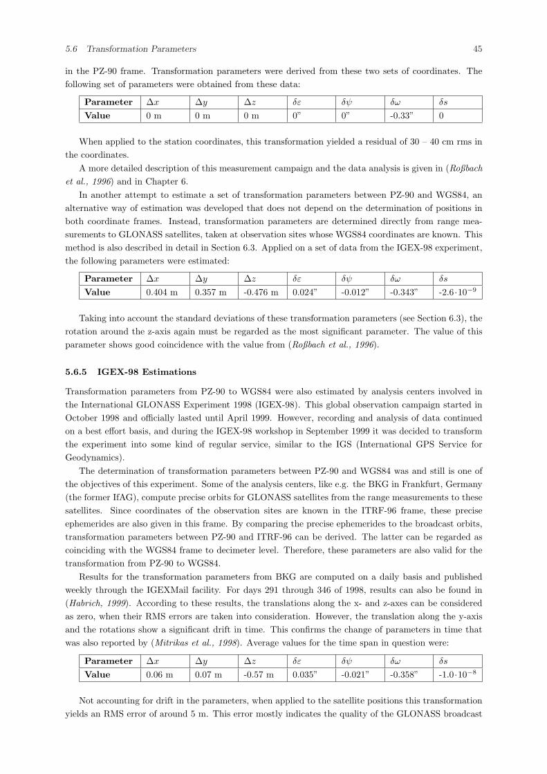
5.6 Transformation Parameters 45
in the PZ-90 frame. Transformation parameters were derived from these two sets of coordinates. Thefollowing set of parameters were obtained from these data:
Parameter ∆x ∆y ∆z δε δψ δω δs
Value 0 m 0 m 0 m 0” 0” -0.33” 0
When applied to the station coordinates, this transformation yielded a residual of 30 – 40 cm rms inthe coordinates.
A more detailed description of this measurement campaign and the data analysis is given in (Roßbachet al., 1996) and in Chapter 6.
In another attempt to estimate a set of transformation parameters between PZ-90 and WGS84, analternative way of estimation was developed that does not depend on the determination of positions inboth coordinate frames. Instead, transformation parameters are determined directly from range mea-surements to GLONASS satellites, taken at observation sites whose WGS84 coordinates are known. Thismethod is also described in detail in Section 6.3. Applied on a set of data from the IGEX-98 experiment,the following parameters were estimated:
Parameter ∆x ∆y ∆z δε δψ δω δs
Value 0.404 m 0.357 m -0.476 m 0.024” -0.012” -0.343” -2.6·10−9
Taking into account the standard deviations of these transformation parameters (see Section 6.3), therotation around the z-axis again must be regarded as the most significant parameter. The value of thisparameter shows good coincidence with the value from (Roßbach et al., 1996).
5.6.5 IGEX-98 Estimations
Transformation parameters from PZ-90 to WGS84 were also estimated by analysis centers involved inthe International GLONASS Experiment 1998 (IGEX-98). This global observation campaign started inOctober 1998 and officially lasted until April 1999. However, recording and analysis of data continuedon a best effort basis, and during the IGEX-98 workshop in September 1999 it was decided to transformthe experiment into some kind of regular service, similar to the IGS (International GPS Service forGeodynamics).
The determination of transformation parameters between PZ-90 and WGS84 was and still is one ofthe objectives of this experiment. Some of the analysis centers, like e.g. the BKG in Frankfurt, Germany(the former IfAG), compute precise orbits for GLONASS satellites from the range measurements to thesesatellites. Since coordinates of the observation sites are known in the ITRF-96 frame, these preciseephemerides are also given in this frame. By comparing the precise ephemerides to the broadcast orbits,transformation parameters between PZ-90 and ITRF-96 can be derived. The latter can be regarded ascoinciding with the WGS84 frame to decimeter level. Therefore, these parameters are also valid for thetransformation from PZ-90 to WGS84.
Results for the transformation parameters from BKG are computed on a daily basis and publishedweekly through the IGEXMail facility. For days 291 through 346 of 1998, results can also be found in(Habrich, 1999). According to these results, the translations along the x- and z-axes can be consideredas zero, when their RMS errors are taken into consideration. However, the translation along the y-axisand the rotations show a significant drift in time. This confirms the change of parameters in time thatwas also reported by (Mitrikas et al., 1998). Average values for the time span in question were:
Parameter ∆x ∆y ∆z δε δψ δω δs
Value 0.06 m 0.07 m -0.57 m 0.035” -0.021” -0.358” -1.0·10−8
Not accounting for drift in the parameters, when applied to the satellite positions this transformationyields an RMS error of around 5 m. This error mostly indicates the quality of the GLONASS broadcast
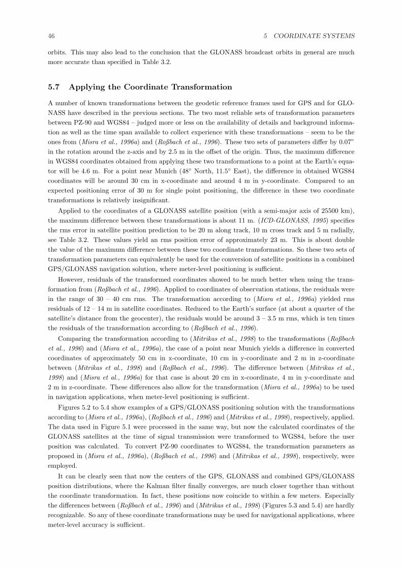
46 5 COORDINATE SYSTEMS
orbits. This may also lead to the conclusion that the GLONASS broadcast orbits in general are muchmore accurate than specified in Table 3.2.
5.7 Applying the Coordinate Transformation
A number of known transformations between the geodetic reference frames used for GPS and for GLO-NASS have described in the previous sections. The two most reliable sets of transformation parametersbetween PZ-90 and WGS84 – judged more or less on the availability of details and background informa-tion as well as the time span available to collect experience with these transformations – seem to be theones from (Misra et al., 1996a) and (Roßbach et al., 1996). These two sets of parameters differ by 0.07”in the rotation around the z-axis and by 2.5 m in the offset of the origin. Thus, the maximum differencein WGS84 coordinates obtained from applying these two transformations to a point at the Earth’s equa-tor will be 4.6 m. For a point near Munich (48◦ North, 11.5◦ East), the difference in obtained WGS84coordinates will be around 30 cm in x-coordinate and around 4 m in y-coordinate. Compared to anexpected positioning error of 30 m for single point positioning, the difference in these two coordinatetransformations is relatively insignificant.
Applied to the coordinates of a GLONASS satellite position (with a semi-major axis of 25500 km),the maximum difference between these transformations is about 11 m. (ICD-GLONASS, 1995) specifiesthe rms error in satellite position prediction to be 20 m along track, 10 m cross track and 5 m radially,see Table 3.2. These values yield an rms position error of approximately 23 m. This is about doublethe value of the maximum difference between these two coordinate transformations. So these two sets oftransformation parameters can equivalently be used for the conversion of satellite positions in a combinedGPS/GLONASS navigation solution, where meter-level positioning is sufficient.
However, residuals of the transformed coordinates showed to be much better when using the trans-formation from (Roßbach et al., 1996). Applied to coordinates of observation stations, the residuals werein the range of 30 – 40 cm rms. The transformation according to (Misra et al., 1996a) yielded rmsresiduals of 12 – 14 m in satellite coordinates. Reduced to the Earth’s surface (at about a quarter of thesatellite’s distance from the geocenter), the residuals would be around 3 – 3.5 m rms, which is ten timesthe residuals of the transformation according to (Roßbach et al., 1996).
Comparing the transformation according to (Mitrikas et al., 1998) to the transformations (Roßbachet al., 1996) and (Misra et al., 1996a), the case of a point near Munich yields a difference in convertedcoordinates of approximately 50 cm in x-coordinate, 10 cm in y-coordinate and 2 m in z-coordinatebetween (Mitrikas et al., 1998) and (Roßbach et al., 1996). The difference between (Mitrikas et al.,1998) and (Misra et al., 1996a) for that case is about 20 cm in x-coordinate, 4 m in y-coordinate and2 m in z-coordinate. These differences also allow for the transformation (Misra et al., 1996a) to be usedin navigation applications, when meter-level positioning is sufficient.
Figures 5.2 to 5.4 show examples of a GPS/GLONASS positioning solution with the transformationsaccording to (Misra et al., 1996a), (Roßbach et al., 1996) and (Mitrikas et al., 1998), respectively, applied.The data used in Figure 5.1 were processed in the same way, but now the calculated coordinates of theGLONASS satellites at the time of signal transmission were transformed to WGS84, before the userposition was calculated. To convert PZ-90 coordinates to WGS84, the transformation parameters asproposed in (Misra et al., 1996a), (Roßbach et al., 1996) and (Mitrikas et al., 1998), respectively, wereemployed.
It can be clearly seen that now the centers of the GPS, GLONASS and combined GPS/GLONASSposition distributions, where the Kalman filter finally converges, are much closer together than withoutthe coordinate transformation. In fact, these positions now coincide to within a few meters. Especiallythe differences between (Roßbach et al., 1996) and (Mitrikas et al., 1998) (Figures 5.3 and 5.4) are hardlyrecognizable. So any of these coordinate transformations may be used for navigational applications, wheremeter-level accuracy is sufficient.

5.7 Applying the Coordinate Transformation 47
Position Deviation [m] from Center E 11� 37’ 41.661” N 48� 04’ 40.598”
◦ GPS × GLONASS ¦ GPS+GLONASS
East/West Deviation [m]
-45 -36 -27 -18 -9 0 9 18 27 36 45
Nor
th/S
outh
Dev
iati
on[m
]
-45
-36
-27
-18
-9
0
9
18
27
36
45
◦
◦◦◦◦◦◦◦◦◦◦◦◦◦◦◦◦◦◦◦◦◦◦◦◦
◦◦◦◦◦◦◦◦◦◦◦◦◦◦◦◦◦◦◦◦◦◦◦◦◦◦◦◦◦◦◦◦◦◦◦◦◦◦◦◦◦◦◦◦◦◦◦◦◦◦◦◦◦◦◦◦◦◦◦◦◦◦◦◦◦◦◦◦◦◦◦◦◦◦◦◦◦◦◦◦◦◦◦◦◦◦◦◦◦◦◦◦◦◦◦◦◦◦◦◦◦◦◦◦◦◦◦◦◦◦◦◦◦◦◦◦◦◦◦◦◦◦◦◦◦◦◦◦◦◦◦◦◦◦◦◦◦◦◦◦◦◦◦◦◦◦◦◦◦◦◦◦◦◦◦◦◦◦◦◦◦◦◦◦◦◦◦◦◦◦◦◦◦◦◦◦◦◦◦◦◦◦◦◦◦◦◦◦◦◦◦◦◦◦◦◦◦◦◦◦◦◦◦◦◦◦◦◦◦◦◦◦◦◦◦◦◦◦◦◦◦◦◦◦◦◦◦◦◦◦◦◦◦◦◦◦◦◦◦◦◦◦◦◦◦◦◦◦◦◦◦◦◦◦◦◦◦◦◦◦◦◦◦◦◦◦◦◦◦◦◦◦◦◦◦◦◦◦◦◦◦◦◦◦◦◦◦◦◦◦◦◦◦◦◦◦◦◦◦◦◦◦◦◦◦◦◦◦◦◦◦◦◦◦◦◦◦◦◦◦◦◦◦◦◦◦◦◦◦◦◦◦◦◦◦◦◦◦◦◦◦◦◦◦◦◦◦◦◦◦◦◦◦◦◦◦◦◦◦◦◦◦◦◦◦◦◦◦◦◦◦◦◦◦◦◦◦◦◦◦◦◦◦◦◦◦◦◦◦◦◦◦◦◦◦◦◦◦◦◦◦◦◦◦◦◦◦◦◦◦◦◦◦◦◦◦◦◦◦◦◦◦◦◦◦◦◦◦◦◦◦◦◦◦◦◦◦◦◦◦◦◦◦◦◦◦◦◦◦◦◦◦◦◦◦◦◦◦◦◦◦◦◦◦◦◦◦◦◦◦◦◦◦◦◦◦◦◦◦◦◦◦◦◦◦◦◦◦◦◦◦◦◦◦◦◦◦◦◦◦◦◦◦◦◦◦◦◦
◦◦◦◦◦◦◦◦◦◦◦◦◦◦◦◦◦◦◦◦◦◦◦◦◦◦◦◦◦◦◦◦◦◦◦◦◦◦◦◦◦◦◦◦◦◦◦◦◦◦◦◦◦◦◦◦◦◦◦◦◦◦◦◦◦◦◦◦◦◦◦◦◦◦◦◦◦◦◦◦◦◦◦◦◦◦◦◦◦◦◦◦◦◦◦◦◦◦◦◦◦◦◦◦◦◦◦◦◦◦◦◦◦◦◦◦◦◦◦◦◦◦◦◦◦◦◦◦◦◦◦◦◦◦◦◦◦◦◦◦◦◦◦◦◦◦◦◦◦◦◦◦◦◦◦◦◦◦◦◦◦◦◦◦◦◦◦◦◦◦◦◦◦◦◦◦◦◦◦◦◦◦◦◦◦◦◦◦◦◦◦◦◦◦◦◦◦◦◦◦◦◦◦◦◦◦◦◦◦◦◦◦◦◦◦◦◦◦◦◦◦◦◦◦◦◦◦◦◦◦◦◦◦◦◦◦◦◦◦◦◦◦◦◦◦◦◦◦◦◦◦◦◦◦◦◦◦◦◦◦◦◦◦◦◦◦◦◦◦◦◦◦◦◦◦◦◦◦◦◦◦◦◦◦◦◦◦◦◦◦◦◦◦◦◦◦◦◦◦◦◦◦◦◦◦◦◦◦◦◦◦◦◦◦◦◦◦◦◦◦◦◦◦◦◦◦◦◦◦◦◦◦◦◦◦◦◦◦◦◦◦◦◦◦◦◦◦◦◦◦◦◦◦◦◦◦◦◦◦◦◦◦◦◦◦◦◦◦◦◦◦◦◦◦◦◦◦◦◦◦◦◦◦◦◦◦◦◦◦◦◦◦◦◦◦◦◦◦◦◦◦◦◦◦◦◦◦◦◦◦◦◦◦◦◦◦◦◦◦◦◦◦◦◦◦◦◦◦◦◦◦◦◦◦◦◦◦◦◦◦◦◦◦◦◦◦◦◦◦◦◦◦◦◦◦◦◦◦◦◦◦◦◦◦◦◦◦◦◦◦◦◦◦◦◦◦◦◦◦◦◦◦◦◦◦◦◦◦◦◦◦◦◦◦◦◦◦◦◦◦◦◦◦◦◦◦◦◦◦◦◦◦◦◦◦◦◦◦◦◦◦◦◦◦◦◦◦◦◦◦◦◦◦◦◦◦◦◦◦◦◦◦◦◦◦◦◦◦◦◦◦◦◦◦◦◦◦◦◦◦◦◦◦◦◦◦◦◦◦◦◦◦◦◦◦◦◦◦◦◦◦◦◦◦◦◦◦◦◦◦◦◦◦◦◦◦◦◦◦◦◦◦◦◦◦◦◦◦◦◦◦◦◦◦◦◦◦◦◦◦◦◦◦◦◦◦◦◦◦◦◦◦◦◦◦◦◦◦◦◦◦◦◦◦◦◦◦◦◦◦◦◦◦◦◦◦◦◦◦◦◦◦◦◦◦◦◦◦◦◦◦◦◦◦◦◦◦◦◦◦◦◦◦◦◦◦◦◦◦◦◦◦◦◦◦◦◦◦◦◦◦◦◦◦◦◦◦◦◦◦◦◦◦◦◦◦◦◦◦◦◦◦◦◦◦◦◦◦◦◦◦◦◦◦◦◦◦◦◦◦◦◦◦◦◦◦◦◦◦◦◦◦◦◦◦◦◦◦◦◦◦◦◦◦◦◦◦◦◦◦◦◦◦◦◦◦◦◦◦◦◦◦◦◦◦◦◦◦◦◦◦◦◦◦◦◦◦◦◦◦◦◦◦◦◦◦◦◦◦◦◦◦◦◦◦◦◦◦◦◦◦◦◦◦◦◦◦◦◦◦◦◦◦◦◦◦◦◦◦◦◦◦◦◦◦◦◦◦◦◦◦◦◦◦◦◦◦◦◦◦◦◦◦◦◦◦◦◦◦◦◦◦◦◦◦◦◦◦◦◦◦◦◦◦◦◦◦◦◦◦◦◦◦◦◦◦◦◦◦◦◦◦◦◦◦◦◦◦◦◦◦◦◦◦◦◦◦◦◦◦◦◦◦◦◦◦◦◦◦◦◦◦◦◦◦◦◦◦◦◦◦◦◦◦◦◦◦◦◦◦◦◦◦◦◦◦◦◦◦◦◦◦◦◦◦◦◦◦◦◦◦◦◦◦◦◦◦◦◦◦◦◦◦◦◦◦◦◦◦◦◦◦◦◦◦◦◦◦◦◦◦◦◦◦◦◦◦◦◦◦◦◦◦◦◦◦◦◦◦◦◦◦◦◦◦◦◦◦◦◦◦◦◦◦◦◦◦◦◦◦◦◦◦◦◦◦◦◦◦◦◦◦◦◦◦◦◦◦◦◦◦◦◦◦◦◦◦◦◦◦◦◦◦◦◦◦◦◦◦◦◦◦◦◦◦◦◦◦◦◦◦◦◦◦◦◦◦◦◦◦◦◦◦◦◦◦◦◦◦◦◦◦◦◦◦◦◦◦◦◦◦◦◦◦◦◦◦◦◦◦◦◦◦◦◦◦◦◦◦◦◦◦◦◦◦◦◦◦◦◦◦◦◦◦◦◦◦◦◦◦◦◦◦◦◦◦◦◦◦◦◦◦◦◦◦◦◦◦◦◦◦◦◦◦◦◦◦◦◦◦◦◦◦◦◦◦◦◦◦◦◦◦◦◦◦◦◦◦◦◦◦◦◦◦◦◦◦◦◦◦◦◦◦◦◦◦◦◦◦◦◦◦◦◦◦◦◦◦◦◦
◦◦◦◦◦◦◦◦◦◦◦◦◦◦◦◦◦◦◦◦◦◦◦◦◦◦◦◦◦◦◦◦◦◦◦◦◦◦◦◦◦◦◦◦◦◦◦◦◦◦◦◦◦◦◦◦◦◦◦◦◦◦◦◦◦◦◦◦◦◦◦◦◦◦◦◦◦◦◦◦◦◦◦◦◦◦◦◦◦◦◦◦◦◦◦◦◦◦◦◦◦◦◦◦◦◦◦◦◦◦◦◦◦◦◦◦◦◦◦◦◦◦◦◦◦◦◦◦◦◦◦◦◦◦◦◦◦◦◦◦◦◦◦◦◦◦◦◦◦◦◦◦◦◦◦◦◦◦◦◦◦◦◦◦◦◦◦◦◦◦◦◦◦◦◦◦◦◦◦◦◦◦◦◦◦◦◦◦◦◦◦◦◦◦◦◦◦◦◦◦◦◦◦◦◦◦◦◦◦◦◦◦◦◦◦◦◦◦◦◦◦◦◦◦◦◦◦◦◦◦◦◦◦◦◦◦◦◦◦◦◦◦◦◦◦◦◦◦◦◦◦◦◦◦◦◦◦◦◦◦◦◦◦◦◦◦◦◦◦◦◦◦◦◦◦◦◦◦◦◦◦◦◦◦◦◦◦◦◦◦◦◦◦◦◦◦◦◦◦◦◦◦◦◦◦◦◦◦◦◦◦◦◦◦◦◦◦◦◦◦◦◦◦◦◦◦◦◦◦◦◦◦◦◦◦◦◦◦◦◦◦◦◦◦◦◦◦◦◦◦◦◦◦◦◦◦◦◦◦◦◦◦◦◦◦◦◦◦◦◦◦◦◦◦◦◦◦◦◦◦◦◦◦◦◦◦◦◦◦◦◦◦◦◦◦◦◦◦◦◦◦◦◦◦◦◦◦◦◦◦◦◦◦◦◦◦◦◦◦◦◦◦◦◦◦◦◦◦◦◦◦◦◦◦◦◦◦◦◦◦◦◦◦◦◦◦◦◦◦◦◦◦◦◦◦◦◦◦◦◦◦◦◦◦◦◦◦◦◦◦◦◦◦◦◦◦◦◦◦◦◦◦◦◦◦◦◦◦◦◦◦◦◦◦◦◦◦◦◦◦◦◦◦◦◦◦◦◦◦◦◦◦◦◦◦◦◦◦◦◦◦◦◦◦◦◦◦◦◦◦◦◦◦◦◦◦◦◦◦◦◦◦◦◦◦◦◦◦◦◦◦◦◦◦◦◦◦◦◦◦◦◦◦◦◦◦◦◦◦◦◦◦◦◦◦◦◦◦◦◦◦◦◦◦◦◦◦◦◦◦◦◦◦◦◦◦◦◦◦◦◦◦◦◦◦◦◦◦◦◦◦◦◦◦◦◦◦◦◦◦◦◦◦◦◦◦◦◦◦◦◦◦◦◦◦◦◦◦◦◦◦◦◦◦◦◦◦◦◦◦◦◦◦◦◦◦◦◦◦◦◦◦◦◦◦◦◦◦◦◦◦◦◦◦◦◦◦◦◦◦◦◦◦◦◦◦◦◦◦◦◦◦◦◦◦◦◦◦◦◦◦◦◦◦◦◦◦◦◦◦◦◦◦◦◦◦◦◦◦◦◦◦◦◦◦◦◦◦◦◦◦◦◦◦◦◦◦◦◦◦◦◦◦◦◦◦◦◦◦◦◦◦◦◦◦◦◦◦◦◦◦◦◦◦◦◦◦◦◦◦◦◦◦◦◦◦◦◦◦◦◦◦◦◦◦◦◦◦◦◦◦◦◦◦◦◦◦◦◦◦◦◦◦◦◦◦◦◦◦◦◦◦◦◦◦◦◦◦◦◦◦◦◦◦◦◦◦◦◦◦◦◦◦◦◦◦◦◦◦◦◦◦◦◦◦◦◦◦◦◦◦◦◦◦◦◦◦◦◦◦◦◦◦◦◦◦◦◦◦◦◦◦◦◦◦◦◦◦◦◦◦◦◦◦◦◦◦◦◦◦◦◦◦◦◦◦◦◦◦◦◦◦◦◦◦◦◦◦◦◦◦◦◦◦◦◦◦◦◦◦◦◦◦◦◦◦◦◦◦◦◦◦◦◦◦◦◦◦◦◦◦◦◦◦◦◦◦◦◦◦◦◦◦◦◦◦◦◦◦◦◦◦◦◦◦◦◦◦◦◦◦◦◦◦◦◦◦◦◦◦◦◦◦◦◦◦◦◦◦◦◦◦◦◦◦◦◦◦◦◦◦◦◦◦◦◦◦◦◦◦◦◦◦◦◦◦◦◦◦◦◦◦◦◦◦◦◦◦◦◦◦◦◦◦◦◦◦◦◦◦◦◦◦◦◦◦◦◦◦◦◦◦◦◦◦◦◦◦◦◦◦◦◦◦◦◦◦◦◦◦◦◦◦◦◦◦◦◦◦◦◦◦◦◦◦◦◦◦◦◦◦◦◦◦◦◦◦◦◦◦◦◦◦◦◦◦◦◦◦◦◦◦◦◦◦◦◦◦◦◦◦◦◦◦◦◦◦◦◦◦◦◦◦◦◦◦◦◦◦◦◦◦◦◦◦◦◦◦◦◦◦◦◦◦◦◦◦◦◦◦◦◦◦◦◦◦◦◦◦◦◦◦◦◦◦◦◦◦◦◦◦◦◦◦◦◦◦◦◦◦◦◦◦◦◦◦◦◦◦◦◦◦◦◦◦◦◦◦◦◦◦◦◦◦◦◦◦◦◦◦◦◦◦◦◦◦◦◦◦◦◦◦◦◦◦◦◦◦◦◦◦◦◦◦◦◦◦◦◦◦◦◦◦◦◦◦◦◦◦◦◦◦◦◦◦◦◦◦◦◦◦◦◦◦◦◦◦◦◦◦◦◦◦◦◦◦◦◦◦◦◦◦◦◦◦◦◦◦◦◦◦◦◦◦◦◦◦◦◦◦◦◦◦◦◦◦◦◦◦◦◦◦◦◦◦◦◦◦◦◦◦◦◦◦◦◦◦◦◦◦◦◦◦◦◦◦◦◦◦◦◦◦◦◦◦◦◦◦◦◦◦◦◦◦◦◦◦◦◦◦◦◦◦◦◦◦◦◦◦◦◦◦◦◦◦◦◦◦◦◦◦◦◦◦◦◦◦◦◦◦◦◦◦◦◦◦◦◦◦◦◦◦◦◦◦◦◦◦◦◦◦◦◦◦◦◦◦◦◦◦◦◦◦◦◦◦◦◦◦
××××××××××××××××××××××××××××××××××××××××××××××××××××××××××××××××××××××××××××××××××××××××××××××××××××××××××××××××××××××××××××××××××××××××××××××××××××××××××××××××××××××××××××××××××××××××××××××××××××××××××××××××××××××××××××××××××××××××××××××××××××××××××××××××××××××××××××××××××××××××××××××××××××××××××××××××××××××××××××××××××××××××××××××××××××××××××××××××××××××××××××××××××××××××××××××××××××××××××××××××××××××××××××××××××××××××××××××××××××××××××××××××××××××××××××××××××××××××××××××××××××××××××××××××××××××××××××××××××××××××××××××××××××××××××××××××××××××××××××××××××××××××××××××××××××××××××××××××××××××××××××××××××××××××××××××××××××××××××××××××××××××××××××××××××××××××××××××××××××××××××××××××××××××××××××××××××××××××××××××××××××××××××××××××××××××××××××××××××××××××××××××××××××××××××××××××××××××××××××××××××××
¦
¦
¦
¦¦¦¦¦¦¦¦¦¦¦¦¦¦¦¦¦¦¦¦¦¦¦¦¦¦¦
¦¦¦¦¦¦¦¦¦¦¦¦¦¦¦¦¦¦¦¦¦¦¦¦¦¦¦¦¦¦¦¦¦
¦¦¦¦¦¦¦¦¦¦¦¦¦¦¦¦¦¦¦¦¦¦¦¦¦¦¦¦¦¦¦¦¦¦¦¦¦¦¦¦¦¦¦¦¦¦¦¦¦¦¦¦¦¦¦¦¦¦¦¦¦¦¦¦¦¦¦¦¦¦¦¦¦¦¦¦¦¦¦¦¦¦¦¦¦¦¦¦¦¦¦¦¦¦¦¦¦¦¦¦¦¦¦¦¦¦¦¦¦¦¦¦¦¦¦¦¦¦¦¦¦¦¦¦¦¦¦¦¦¦¦¦¦¦¦¦¦¦¦¦¦¦¦¦¦¦¦¦¦¦¦¦¦¦¦¦¦¦¦¦¦¦¦¦¦¦¦¦¦¦¦¦¦¦¦¦¦¦¦¦¦¦¦¦¦¦¦¦¦¦¦¦¦¦¦¦¦¦¦¦¦¦¦¦¦¦¦¦¦¦¦¦¦¦¦¦¦¦¦¦¦¦¦¦¦¦¦¦¦¦¦¦¦¦¦¦¦¦¦¦¦¦¦¦¦¦¦¦¦¦¦¦¦¦¦¦¦¦¦¦¦¦¦¦¦¦¦¦¦¦¦¦¦¦¦¦¦¦¦¦¦¦¦¦¦¦¦¦¦¦¦¦¦¦¦¦¦¦¦¦¦¦¦¦¦¦¦¦¦¦¦¦¦¦¦¦¦¦¦¦¦¦¦¦¦¦¦¦¦¦¦¦¦¦¦¦¦¦¦¦¦¦¦¦¦¦¦¦¦¦¦¦¦¦¦¦¦¦¦¦¦¦¦¦¦¦¦¦¦¦¦¦¦¦¦¦¦¦¦¦¦¦¦¦¦¦¦¦¦¦¦¦¦¦¦¦¦¦¦¦¦¦¦¦¦¦¦¦¦¦¦¦¦¦¦¦¦¦¦¦¦¦¦¦¦¦¦¦¦¦¦¦¦¦¦¦¦¦¦¦¦¦¦¦¦¦¦¦¦¦¦¦¦¦¦¦¦¦¦¦¦¦¦¦¦¦¦¦¦¦¦¦¦¦¦¦¦¦¦¦¦¦¦¦¦¦¦¦¦¦¦¦¦¦¦¦¦¦¦¦¦¦¦¦¦¦¦¦¦¦¦¦¦¦¦¦¦¦¦¦¦¦¦¦¦¦¦¦¦¦¦¦¦¦¦¦¦¦¦¦¦¦¦¦¦¦¦¦¦¦¦¦¦¦¦¦¦¦¦¦¦¦¦¦¦¦¦¦¦¦¦¦¦¦¦¦¦¦¦¦¦¦¦¦¦¦¦¦¦¦¦¦¦¦¦¦¦¦¦¦¦¦¦¦¦¦¦¦¦¦¦¦¦¦¦¦¦¦¦¦¦¦¦¦¦¦¦¦¦¦¦¦¦¦¦¦¦¦¦¦¦¦¦¦¦¦¦¦¦¦¦¦¦¦¦¦¦¦¦¦¦¦¦¦¦¦¦¦¦¦¦¦¦¦¦¦¦¦¦¦¦¦¦¦¦¦¦¦¦¦¦¦¦¦¦¦¦¦¦¦¦¦¦¦¦¦¦¦¦¦¦¦¦¦¦¦¦¦¦¦¦¦¦¦¦¦¦¦¦¦¦¦¦¦¦¦¦¦¦¦¦¦¦¦¦¦¦¦¦¦¦¦¦¦¦¦¦¦¦¦¦¦¦¦¦¦¦¦¦¦¦¦¦¦¦¦¦¦¦¦¦¦¦¦¦¦¦¦¦¦¦¦¦¦¦¦¦¦¦¦¦¦¦¦¦¦¦¦¦¦¦¦¦¦¦¦¦¦¦¦¦¦¦¦¦¦¦¦¦¦¦¦¦¦¦¦¦¦¦¦¦¦¦¦¦¦¦¦¦¦¦¦¦¦¦¦¦¦¦¦¦¦¦¦¦¦¦¦¦¦¦¦¦¦¦¦¦¦¦¦¦¦¦¦¦¦¦¦¦¦¦¦¦¦¦¦¦¦¦¦¦¦¦¦¦¦¦¦¦¦¦¦¦¦¦¦¦¦¦¦¦¦¦¦¦¦¦¦¦¦¦¦¦¦¦¦¦¦¦¦¦¦¦¦¦¦¦¦¦¦¦¦¦¦¦¦¦¦¦¦¦¦¦¦¦¦¦¦¦¦¦¦¦¦¦¦¦¦¦¦¦¦¦¦¦¦¦¦¦¦¦¦¦¦¦¦¦¦¦¦¦¦¦¦¦¦¦¦¦¦¦¦¦¦¦¦¦¦¦¦¦¦¦¦¦¦¦¦¦¦¦¦¦¦¦¦¦¦¦¦¦¦¦¦¦¦¦¦¦¦¦¦¦¦¦¦¦¦¦¦¦¦¦¦¦¦¦¦¦¦¦¦¦¦¦¦¦¦¦¦¦¦¦¦¦¦¦¦¦¦¦¦¦¦¦¦¦¦¦¦¦¦¦¦¦¦¦¦¦¦¦¦¦¦¦¦¦¦¦¦¦¦¦¦¦¦¦¦¦¦¦¦¦¦¦¦¦¦¦¦¦¦¦¦¦¦¦¦¦¦¦¦¦¦¦¦¦¦¦¦¦¦¦¦¦¦¦¦¦¦¦¦¦¦¦¦¦¦¦¦¦¦¦¦¦¦¦¦¦¦¦¦¦¦¦¦¦¦¦¦¦¦¦¦¦¦¦¦¦¦¦¦¦¦¦¦¦¦¦¦¦¦¦¦¦¦¦¦¦¦¦¦¦¦¦¦¦¦¦¦¦¦¦¦¦¦¦¦¦¦¦¦¦¦¦¦¦¦¦¦¦¦¦¦¦¦¦¦¦¦¦¦¦¦¦¦¦¦¦¦¦¦¦¦¦¦¦¦¦¦¦¦¦¦¦¦¦¦¦¦¦¦¦¦¦¦¦¦¦¦¦¦¦¦¦¦¦¦¦¦¦¦¦¦¦¦¦¦¦¦¦¦¦¦¦¦¦¦¦¦¦¦¦¦¦¦¦¦¦¦¦¦¦¦¦¦¦¦¦¦¦¦¦¦¦¦¦¦¦¦¦¦¦¦¦¦¦¦¦¦¦¦¦¦¦¦¦¦¦¦¦¦¦¦¦¦¦¦¦¦¦¦¦¦¦¦¦¦¦¦¦¦¦¦¦¦¦¦¦¦¦¦¦¦¦¦¦¦¦¦¦¦¦¦¦¦¦¦¦¦¦¦¦¦¦¦¦¦¦¦¦¦¦¦¦¦¦¦¦¦¦¦¦¦¦¦¦¦¦¦¦¦¦¦¦¦¦¦¦¦¦¦¦¦¦¦¦¦¦¦¦¦¦¦¦¦¦¦¦¦¦¦¦¦¦¦¦¦¦¦¦¦¦¦¦¦¦¦¦¦¦¦¦¦¦¦¦¦¦¦¦¦¦¦¦¦¦¦¦¦¦¦¦¦¦¦¦¦¦¦¦¦¦¦¦¦¦¦¦¦¦¦¦¦¦¦¦¦¦¦¦¦¦¦¦¦¦¦¦¦¦¦¦¦¦¦¦¦¦¦¦¦¦¦¦¦¦¦¦¦¦¦¦¦¦¦¦¦¦¦¦¦¦¦¦¦¦¦¦¦¦¦¦¦¦¦¦¦¦¦¦¦¦¦¦¦¦¦¦¦¦¦¦¦¦¦¦¦¦¦¦¦¦¦¦¦¦¦¦¦¦¦¦¦¦¦¦¦¦¦¦¦¦¦¦¦¦¦¦¦¦¦¦¦¦¦¦¦¦¦¦¦¦¦¦¦¦¦¦¦¦¦¦¦¦¦¦¦¦¦¦¦¦¦¦¦¦¦¦¦¦¦¦¦¦¦¦¦¦¦¦¦¦¦¦¦¦¦¦¦¦¦¦¦¦¦¦¦¦¦¦¦¦¦¦¦¦¦¦¦¦¦¦¦¦¦¦¦¦¦¦¦¦¦¦¦¦¦¦¦¦¦¦¦¦¦¦¦¦¦¦¦¦¦¦¦¦¦¦¦¦¦¦¦¦¦¦¦¦¦¦¦¦¦¦¦¦¦¦¦¦¦¦¦¦¦¦¦¦¦¦¦¦¦¦¦¦¦¦¦¦¦¦¦¦¦¦¦¦¦¦¦¦¦¦¦¦¦¦¦¦¦¦¦¦¦¦¦¦¦¦¦¦¦¦¦¦¦¦¦¦¦¦¦¦¦¦¦¦¦¦¦¦¦¦¦¦¦¦¦¦¦¦¦¦¦¦¦¦¦¦¦¦¦¦¦¦¦¦¦¦¦¦¦¦¦¦¦¦¦¦¦¦¦¦¦¦¦¦¦¦¦¦¦¦¦¦¦¦¦¦¦¦¦¦¦¦¦¦¦¦¦¦¦¦¦¦¦¦¦¦¦¦¦¦¦¦¦¦¦¦¦¦¦¦¦¦¦¦¦¦¦¦¦¦¦¦¦¦¦¦¦¦¦¦¦¦¦¦¦¦¦¦¦¦¦¦¦¦¦¦¦¦¦¦¦¦¦¦¦¦¦¦¦¦¦¦¦¦¦¦¦¦¦¦¦¦¦¦¦¦¦¦¦¦¦¦¦¦¦¦¦¦¦¦¦¦¦¦¦¦¦¦¦¦¦¦¦¦¦¦¦¦¦¦¦¦¦¦¦¦¦¦¦¦¦¦¦¦¦¦¦¦¦¦¦¦¦¦¦¦¦¦¦¦¦¦¦¦¦¦¦¦¦¦¦¦¦¦¦¦¦¦¦¦¦¦¦¦¦¦¦¦¦¦¦¦¦¦¦¦¦¦¦¦¦¦¦¦¦¦¦¦¦¦¦¦¦¦¦¦¦¦¦¦¦¦¦¦¦¦¦¦¦¦¦¦¦¦¦¦¦¦¦¦¦¦¦¦¦¦¦¦¦¦¦¦¦¦¦¦¦¦¦¦¦¦¦¦¦¦¦¦¦¦¦¦¦¦¦¦¦¦¦¦¦¦¦¦¦¦¦¦¦¦¦¦¦¦¦¦¦¦¦¦¦¦¦¦¦¦¦¦¦¦¦¦¦¦¦¦¦¦¦¦¦¦¦¦¦¦¦¦¦¦¦¦¦¦¦¦¦¦¦¦¦¦¦¦¦¦¦¦¦¦¦¦¦¦¦¦¦¦¦¦¦¦¦¦¦¦¦¦¦¦¦¦¦¦¦¦¦¦¦¦¦¦¦¦¦¦¦¦¦¦¦¦¦¦¦¦¦¦¦¦¦¦¦¦¦¦¦¦¦¦¦¦¦¦¦¦¦¦¦¦¦¦¦¦¦¦¦¦¦¦¦¦¦¦¦¦¦¦¦¦¦¦¦¦¦¦¦¦¦¦¦¦¦¦¦¦¦¦¦¦¦¦¦¦¦¦¦¦¦¦¦¦¦¦¦¦¦¦¦¦¦¦¦¦¦¦¦¦¦¦¦¦¦¦¦¦¦¦¦¦¦¦¦¦¦¦¦¦¦¦¦¦¦¦¦¦¦¦¦¦¦¦¦¦¦¦¦¦¦¦¦¦¦¦¦¦¦¦¦¦¦¦¦¦¦¦¦¦¦¦¦¦¦¦¦¦¦¦¦¦¦¦¦¦¦¦¦¦¦¦¦¦¦¦¦¦¦¦¦¦¦¦¦¦¦¦¦¦¦¦¦¦¦¦¦¦¦¦¦¦¦¦¦
¦¦¦¦¦¦¦¦¦¦¦¦¦¦¦¦¦¦¦¦¦¦¦¦¦¦¦¦¦¦¦¦¦¦¦¦¦¦¦¦¦¦¦¦¦¦¦¦¦¦¦¦¦¦¦¦¦¦¦¦¦¦¦¦¦¦¦¦¦¦¦¦¦¦¦¦¦¦¦¦¦¦¦¦¦¦¦¦¦¦¦
Figure 5.2: Example of combined GPS/GLONASS positioning with coordinate transformation accordingto (Misra et al., 1996a).
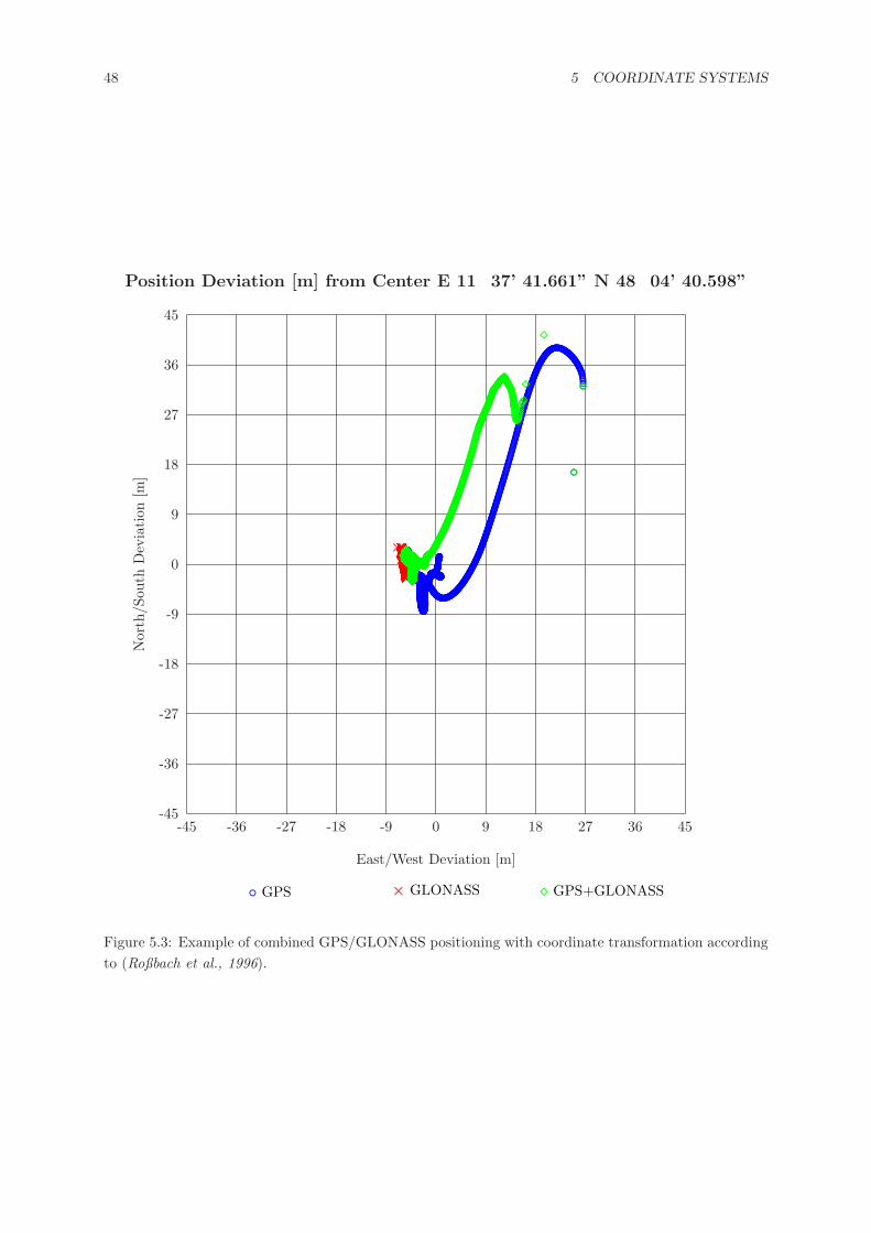
48 5 COORDINATE SYSTEMS
Position Deviation [m] from Center E 11� 37’ 41.661” N 48� 04’ 40.598”
◦ GPS × GLONASS ¦ GPS+GLONASS
East/West Deviation [m]
-45 -36 -27 -18 -9 0 9 18 27 36 45
Nor
th/S
outh
Dev
iati
on[m
]
-45
-36
-27
-18
-9
0
9
18
27
36
45
◦
◦◦◦◦◦◦◦◦◦◦◦◦◦◦◦◦◦◦◦◦◦◦◦◦
◦◦◦◦◦◦◦◦◦◦◦◦◦◦◦◦◦◦◦◦◦◦◦◦◦◦◦◦◦◦◦◦◦◦◦◦◦◦◦◦◦◦◦◦◦◦◦◦◦◦◦◦◦◦◦◦◦◦◦◦◦◦◦◦◦◦◦◦◦◦◦◦◦◦◦◦◦◦◦◦◦◦◦◦◦◦◦◦◦◦◦◦◦◦◦◦◦◦◦◦◦◦◦◦◦◦◦◦◦◦◦◦◦◦◦◦◦◦◦◦◦◦◦◦◦◦◦◦◦◦◦◦◦◦◦◦◦◦◦◦◦◦◦◦◦◦◦◦◦◦◦◦◦◦◦◦◦◦◦◦◦◦◦◦◦◦◦◦◦◦◦◦◦◦◦◦◦◦◦◦◦◦◦◦◦◦◦◦◦◦◦◦◦◦◦◦◦◦◦◦◦◦◦◦◦◦◦◦◦◦◦◦◦◦◦◦◦◦◦◦◦◦◦◦◦◦◦◦◦◦◦◦◦◦◦◦◦◦◦◦◦◦◦◦◦◦◦◦◦◦◦◦◦◦◦◦◦◦◦◦◦◦◦◦◦◦◦◦◦◦◦◦◦◦◦◦◦◦◦◦◦◦◦◦◦◦◦◦◦◦◦◦◦◦◦◦◦◦◦◦◦◦◦◦◦◦◦◦◦◦◦◦◦◦◦◦◦◦◦◦◦◦◦◦◦◦◦◦◦◦◦◦◦◦◦◦◦◦◦◦◦◦◦◦◦◦◦◦◦◦◦◦◦◦◦◦◦◦◦◦◦◦◦◦◦◦◦◦◦◦◦◦◦◦◦◦◦◦◦◦◦◦◦◦◦◦◦◦◦◦◦◦◦◦◦◦◦◦◦◦◦◦◦◦◦◦◦◦◦◦◦◦◦◦◦◦◦◦◦◦◦◦◦◦◦◦◦◦◦◦◦◦◦◦◦◦◦◦◦◦◦◦◦◦◦◦◦◦◦◦◦◦◦◦◦◦◦◦◦◦◦◦◦◦◦◦◦◦◦◦◦◦◦◦◦◦◦◦◦◦◦◦◦◦◦◦◦◦◦◦◦◦◦◦◦◦◦◦◦◦◦◦◦◦◦◦◦◦
◦◦◦◦◦◦◦◦◦◦◦◦◦◦◦◦◦◦◦◦◦◦◦◦◦◦◦◦◦◦◦◦◦◦◦◦◦◦◦◦◦◦◦◦◦◦◦◦◦◦◦◦◦◦◦◦◦◦◦◦◦◦◦◦◦◦◦◦◦◦◦◦◦◦◦◦◦◦◦◦◦◦◦◦◦◦◦◦◦◦◦◦◦◦◦◦◦◦◦◦◦◦◦◦◦◦◦◦◦◦◦◦◦◦◦◦◦◦◦◦◦◦◦◦◦◦◦◦◦◦◦◦◦◦◦◦◦◦◦◦◦◦◦◦◦◦◦◦◦◦◦◦◦◦◦◦◦◦◦◦◦◦◦◦◦◦◦◦◦◦◦◦◦◦◦◦◦◦◦◦◦◦◦◦◦◦◦◦◦◦◦◦◦◦◦◦◦◦◦◦◦◦◦◦◦◦◦◦◦◦◦◦◦◦◦◦◦◦◦◦◦◦◦◦◦◦◦◦◦◦◦◦◦◦◦◦◦◦◦◦◦◦◦◦◦◦◦◦◦◦◦◦◦◦◦◦◦◦◦◦◦◦◦◦◦◦◦◦◦◦◦◦◦◦◦◦◦◦◦◦◦◦◦◦◦◦◦◦◦◦◦◦◦◦◦◦◦◦◦◦◦◦◦◦◦◦◦◦◦◦◦◦◦◦◦◦◦◦◦◦◦◦◦◦◦◦◦◦◦◦◦◦◦◦◦◦◦◦◦◦◦◦◦◦◦◦◦◦◦◦◦◦◦◦◦◦◦◦◦◦◦◦◦◦◦◦◦◦◦◦◦◦◦◦◦◦◦◦◦◦◦◦◦◦◦◦◦◦◦◦◦◦◦◦◦◦◦◦◦◦◦◦◦◦◦◦◦◦◦◦◦◦◦◦◦◦◦◦◦◦◦◦◦◦◦◦◦◦◦◦◦◦◦◦◦◦◦◦◦◦◦◦◦◦◦◦◦◦◦◦◦◦◦◦◦◦◦◦◦◦◦◦◦◦◦◦◦◦◦◦◦◦◦◦◦◦◦◦◦◦◦◦◦◦◦◦◦◦◦◦◦◦◦◦◦◦◦◦◦◦◦◦◦◦◦◦◦◦◦◦◦◦◦◦◦◦◦◦◦◦◦◦◦◦◦◦◦◦◦◦◦◦◦◦◦◦◦◦◦◦◦◦◦◦◦◦◦◦◦◦◦◦◦◦◦◦◦◦◦◦◦◦◦◦◦◦◦◦◦◦◦◦◦◦◦◦◦◦◦◦◦◦◦◦◦◦◦◦◦◦◦◦◦◦◦◦◦◦◦◦◦◦◦◦◦◦◦◦◦◦◦◦◦◦◦◦◦◦◦◦◦◦◦◦◦◦◦◦◦◦◦◦◦◦◦◦◦◦◦◦◦◦◦◦◦◦◦◦◦◦◦◦◦◦◦◦◦◦◦◦◦◦◦◦◦◦◦◦◦◦◦◦◦◦◦◦◦◦◦◦◦◦◦◦◦◦◦◦◦◦◦◦◦◦◦◦◦◦◦◦◦◦◦◦◦◦◦◦◦◦◦◦◦◦◦◦◦◦◦◦◦◦◦◦◦◦◦◦◦◦◦◦◦◦◦◦◦◦◦◦◦◦◦◦◦◦◦◦◦◦◦◦◦◦◦◦◦◦◦◦◦◦◦◦◦◦◦◦◦◦◦◦◦◦◦◦◦◦◦◦◦◦◦◦◦◦◦◦◦◦◦◦◦◦◦◦◦◦◦◦◦◦◦◦◦◦◦◦◦◦◦◦◦◦◦◦◦◦◦◦◦◦◦◦◦◦◦◦◦◦◦◦◦◦◦◦◦◦◦◦◦◦◦◦◦◦◦◦◦◦◦◦◦◦◦◦◦◦◦◦◦◦◦◦◦◦◦◦◦◦◦◦◦◦◦◦◦◦◦◦◦◦◦◦◦◦◦◦◦◦◦◦◦◦◦◦◦◦◦◦◦◦◦◦◦◦◦◦◦◦◦◦◦◦◦◦◦◦◦◦◦◦◦◦◦◦◦◦◦◦◦◦◦◦◦◦◦◦◦◦◦◦◦◦◦◦◦◦◦◦◦◦◦◦◦◦◦◦◦◦◦◦◦◦◦◦◦◦◦◦◦◦◦◦◦◦◦◦◦◦◦◦◦◦◦◦◦◦◦◦◦◦◦◦◦◦◦◦◦◦◦◦◦◦◦◦◦◦◦◦◦◦◦◦◦◦◦◦◦◦◦◦◦◦◦◦◦◦◦◦◦◦◦◦◦◦◦◦◦◦◦◦◦◦◦◦◦◦◦◦◦◦◦◦◦◦◦◦◦◦◦◦◦◦◦◦◦◦◦◦◦◦◦◦◦◦◦◦◦◦◦◦◦◦◦◦◦◦◦◦◦◦◦◦◦◦◦◦◦◦◦◦◦◦◦◦◦◦◦◦◦◦◦◦◦◦◦◦◦◦◦◦◦◦◦◦◦◦◦◦◦◦◦◦◦◦◦◦◦◦◦◦◦◦◦◦◦◦◦◦◦◦◦◦◦◦◦◦◦◦◦◦◦◦◦◦◦◦◦◦◦◦◦◦◦◦◦◦◦◦◦◦◦◦◦◦◦◦◦◦◦◦◦◦◦◦◦◦◦◦◦◦◦◦◦◦◦◦◦◦◦◦◦◦◦◦◦◦◦◦◦◦◦◦◦◦◦◦◦◦◦◦◦◦◦◦◦◦◦◦
◦◦◦◦◦◦◦◦◦◦◦◦◦◦◦◦◦◦◦◦◦◦◦◦◦◦◦◦◦◦◦◦◦◦◦◦◦◦◦◦◦◦◦◦◦◦◦◦◦◦◦◦◦◦◦◦◦◦◦◦◦◦◦◦◦◦◦◦◦◦◦◦◦◦◦◦◦◦◦◦◦◦◦◦◦◦◦◦◦◦◦◦◦◦◦◦◦◦◦◦◦◦◦◦◦◦◦◦◦◦◦◦◦◦◦◦◦◦◦◦◦◦◦◦◦◦◦◦◦◦◦◦◦◦◦◦◦◦◦◦◦◦◦◦◦◦◦◦◦◦◦◦◦◦◦◦◦◦◦◦◦◦◦◦◦◦◦◦◦◦◦◦◦◦◦◦◦◦◦◦◦◦◦◦◦◦◦◦◦◦◦◦◦◦◦◦◦◦◦◦◦◦◦◦◦◦◦◦◦◦◦◦◦◦◦◦◦◦◦◦◦◦◦◦◦◦◦◦◦◦◦◦◦◦◦◦◦◦◦◦◦◦◦◦◦◦◦◦◦◦◦◦◦◦◦◦◦◦◦◦◦◦◦◦◦◦◦◦◦◦◦◦◦◦◦◦◦◦◦◦◦◦◦◦◦◦◦◦◦◦◦◦◦◦◦◦◦◦◦◦◦◦◦◦◦◦◦◦◦◦◦◦◦◦◦◦◦◦◦◦◦◦◦◦◦◦◦◦◦◦◦◦◦◦◦◦◦◦◦◦◦◦◦◦◦◦◦◦◦◦◦◦◦◦◦◦◦◦◦◦◦◦◦◦◦◦◦◦◦◦◦◦◦◦◦◦◦◦◦◦◦◦◦◦◦◦◦◦◦◦◦◦◦◦◦◦◦◦◦◦◦◦◦◦◦◦◦◦◦◦◦◦◦◦◦◦◦◦◦◦◦◦◦◦◦◦◦◦◦◦◦◦◦◦◦◦◦◦◦◦◦◦◦◦◦◦◦◦◦◦◦◦◦◦◦◦◦◦◦◦◦◦◦◦◦◦◦◦◦◦◦◦◦◦◦◦◦◦◦◦◦◦◦◦◦◦◦◦◦◦◦◦◦◦◦◦◦◦◦◦◦◦◦◦◦◦◦◦◦◦◦◦◦◦◦◦◦◦◦◦◦◦◦◦◦◦◦◦◦◦◦◦◦◦◦◦◦◦◦◦◦◦◦◦◦◦◦◦◦◦◦◦◦◦◦◦◦◦◦◦◦◦◦◦◦◦◦◦◦◦◦◦◦◦◦◦◦◦◦◦◦◦◦◦◦◦◦◦◦◦◦◦◦◦◦◦◦◦◦◦◦◦◦◦◦◦◦◦◦◦◦◦◦◦◦◦◦◦◦◦◦◦◦◦◦◦◦◦◦◦◦◦◦◦◦◦◦◦◦◦◦◦◦◦◦◦◦◦◦◦◦◦◦◦◦◦◦◦◦◦◦◦◦◦◦◦◦◦◦◦◦◦◦◦◦◦◦◦◦◦◦◦◦◦◦◦◦◦◦◦◦◦◦◦◦◦◦◦◦◦◦◦◦◦◦◦◦◦◦◦◦◦◦◦◦◦◦◦◦◦◦◦◦◦◦◦◦◦◦◦◦◦◦◦◦◦◦◦◦◦◦◦◦◦◦◦◦◦◦◦◦◦◦◦◦◦◦◦◦◦◦◦◦◦◦◦◦◦◦◦◦◦◦◦◦◦◦◦◦◦◦◦◦◦◦◦◦◦◦◦◦◦◦◦◦◦◦◦◦◦◦◦◦◦◦◦◦◦◦◦◦◦◦◦◦◦◦◦◦◦◦◦◦◦◦◦◦◦◦◦◦◦◦◦◦◦◦◦◦◦◦◦◦◦◦◦◦◦◦◦◦◦◦◦◦◦◦◦◦◦◦◦◦◦◦◦◦◦◦◦◦◦◦◦◦◦◦◦◦◦◦◦◦◦◦◦◦◦◦◦◦◦◦◦◦◦◦◦◦◦◦◦◦◦◦◦◦◦◦◦◦◦◦◦◦◦◦◦◦◦◦◦◦◦◦◦◦◦◦◦◦◦◦◦◦◦◦◦◦◦◦◦◦◦◦◦◦◦◦◦◦◦◦◦◦◦◦◦◦◦◦◦◦◦◦◦◦◦◦◦◦◦◦◦◦◦◦◦◦◦◦◦◦◦◦◦◦◦◦◦◦◦◦◦◦◦◦◦◦◦◦◦◦◦◦◦◦◦◦◦◦◦◦◦◦◦◦◦◦◦◦◦◦◦◦◦◦◦◦◦◦◦◦◦◦◦◦◦◦◦◦◦◦◦◦◦◦◦◦◦◦◦◦◦◦◦◦◦◦◦◦◦◦◦◦◦◦◦◦◦◦◦◦◦◦◦◦◦◦◦◦◦◦◦◦◦◦◦◦◦◦◦◦◦◦◦◦◦◦◦◦◦◦◦◦◦◦◦◦◦◦◦◦◦◦◦◦◦◦◦◦◦◦◦◦◦◦◦◦◦◦◦◦◦◦◦◦◦◦◦◦◦◦◦◦◦◦◦◦◦◦◦◦◦◦◦◦◦◦◦◦◦◦◦◦◦◦◦◦◦◦◦◦◦◦◦◦◦◦◦◦◦◦◦◦◦◦◦◦◦◦◦◦◦◦◦◦◦◦◦◦◦◦◦◦◦◦◦◦◦◦◦◦◦◦◦◦◦◦◦◦◦◦◦◦◦◦◦◦◦◦◦◦◦◦◦◦◦◦◦◦◦◦◦◦◦◦◦◦◦◦◦◦◦◦◦◦◦◦◦◦◦◦◦◦◦◦◦◦◦◦◦◦◦◦◦◦◦◦◦◦◦◦◦◦◦◦◦◦◦◦◦◦◦◦◦◦◦◦◦◦◦◦◦◦◦◦◦◦◦◦◦◦◦◦◦◦◦◦◦◦◦◦◦◦◦◦◦◦◦◦◦◦◦◦◦◦◦◦◦◦◦◦◦◦◦◦◦◦◦◦◦◦◦◦◦◦◦◦◦◦◦◦◦◦◦◦◦◦◦◦◦◦◦◦◦◦◦◦◦◦◦◦◦◦◦◦◦◦◦◦◦◦◦◦◦◦◦◦◦◦◦◦◦◦◦◦◦◦◦◦◦◦◦◦◦◦◦◦◦◦◦◦◦◦◦◦◦◦◦◦◦◦◦◦◦◦◦◦
×××××××××××××××××××××××××××××××××××××××××××××××××××××××××××××××××××××××××××××××××××××××××××××××××××××××××××××××××××××××××××××××××××××××××××××××××××××××××××××××××××××××××××××××××××××××××××××××××××××××××××××××××××××××××××××××××××××××××××××××××××××××××××××××××××××××××××××××××××××××××××××××××××××××××××××××××××××××××××××××××××××××××××××××××××××××××××××××××××××××××××××××××××××××××××××××××××××××××××××××××××××××××××××××××××××××××××××××××××××××××××××××××××××××××××××××××××××××××××××××××××××××××××××××××××××××××××××××××××××××××××××××××××××××××××××××××××××××××××××××××××××××××××××××××××××××××××××××××××××××××××××××××××××××××××××××××××××××××××××××××××××××××××××××××××××××××××××××××××××××××××××××××××××××××××××××××××××××××××××××××××××××××××××××××××××××××××××××××××××××××××××××××××××××××××××××××××××××××××××××××××××××××××××××
¦
¦
¦
¦¦¦¦¦¦¦¦¦¦¦¦¦¦¦¦¦¦¦¦¦¦¦¦¦¦¦
¦¦¦¦¦¦¦¦¦¦¦¦¦¦¦¦¦¦¦¦¦¦¦¦¦¦¦¦¦¦¦¦¦
¦¦¦¦¦¦¦¦¦¦¦¦¦¦¦¦¦¦¦¦¦¦¦¦¦¦¦¦¦¦¦¦¦¦¦¦¦¦¦¦¦¦¦¦¦¦¦¦¦¦¦¦¦¦¦¦¦¦¦¦¦¦¦¦¦¦¦¦¦¦¦¦¦¦¦¦¦¦¦¦¦¦¦¦¦¦¦¦¦¦¦¦¦¦¦¦¦¦¦¦¦¦¦¦¦¦¦¦¦¦¦¦¦¦¦¦¦¦¦¦¦¦¦¦¦¦¦¦¦¦¦¦¦¦¦¦¦¦¦¦¦¦¦¦¦¦¦¦¦¦¦¦¦¦¦¦¦¦¦¦¦¦¦¦¦¦¦¦¦¦¦¦¦¦¦¦¦¦¦¦¦¦¦¦¦¦¦¦¦¦¦¦¦¦¦¦¦¦¦¦¦¦¦¦¦¦¦¦¦¦¦¦¦¦¦¦¦¦¦¦¦¦¦¦¦¦¦¦¦¦¦¦¦¦¦¦¦¦¦¦¦¦¦¦¦¦¦¦¦¦¦¦¦¦¦¦¦¦¦¦¦¦¦¦¦¦¦¦¦¦¦¦¦¦¦¦¦¦¦¦¦¦¦¦¦¦¦¦¦¦¦¦¦¦¦¦¦¦¦¦¦¦¦¦¦¦¦¦¦¦¦¦¦¦¦¦¦¦¦¦¦¦¦¦¦¦¦¦¦¦¦¦¦¦¦¦¦¦¦¦¦¦¦¦¦¦¦¦¦¦¦¦¦¦¦¦¦¦¦¦¦¦¦¦¦¦¦¦¦¦¦¦¦¦¦¦¦¦¦¦¦¦¦¦¦¦¦¦¦¦¦¦¦¦¦¦¦¦¦¦¦¦¦¦¦¦¦¦¦¦¦¦¦¦¦¦¦¦¦¦¦¦¦¦¦¦¦¦¦¦¦¦¦¦¦¦¦¦¦¦¦¦¦¦¦¦¦¦¦¦¦¦¦¦¦¦¦¦¦¦¦¦¦¦¦¦¦¦¦¦¦¦¦¦¦¦¦¦¦¦¦¦¦¦¦¦¦¦¦¦¦¦¦¦¦¦¦¦¦¦¦¦¦¦¦¦¦¦¦¦¦¦¦¦¦¦¦¦¦¦¦¦¦¦¦¦¦¦¦¦¦¦¦¦¦¦¦¦¦¦¦¦¦¦¦¦¦¦¦¦¦¦¦¦¦¦¦¦¦¦¦¦¦¦¦¦¦¦¦¦¦¦¦¦¦¦¦¦¦¦¦¦¦¦¦¦¦¦¦¦¦¦¦¦¦¦¦¦¦¦¦¦¦¦¦¦¦¦¦¦¦¦¦¦¦¦¦¦¦¦¦¦¦¦¦¦¦¦¦¦¦¦¦¦¦¦¦¦¦¦¦¦¦¦¦¦¦¦¦¦¦¦¦¦¦¦¦¦¦¦¦¦¦¦¦¦¦¦¦¦¦¦¦¦¦¦¦¦¦¦¦¦¦¦¦¦¦¦¦¦¦¦¦¦¦¦¦¦¦¦¦¦¦¦¦¦¦¦¦¦¦¦¦¦¦¦¦¦¦¦¦¦¦¦¦¦¦¦¦¦¦¦¦¦¦¦¦¦¦¦¦¦¦¦¦¦¦¦¦¦¦¦¦¦¦¦¦¦¦¦¦¦¦¦¦¦¦¦¦¦¦¦¦¦¦¦¦¦¦¦¦¦¦¦¦¦¦¦¦¦¦¦¦¦¦¦¦¦¦¦¦¦¦¦¦¦¦¦¦¦¦¦¦¦¦¦¦¦¦¦¦¦¦¦¦¦¦¦¦¦¦¦¦¦¦¦¦¦¦¦¦¦¦¦¦¦¦¦¦¦¦¦¦¦¦¦¦¦¦¦¦¦¦¦¦¦¦¦¦¦¦¦¦¦¦¦¦¦¦¦¦¦¦¦¦¦¦¦¦¦¦¦¦¦¦¦¦¦¦¦¦¦¦¦¦¦¦¦¦¦¦¦¦¦¦¦¦¦¦¦¦¦¦¦¦¦¦¦¦¦¦¦¦¦¦¦¦¦¦¦¦¦¦¦¦¦¦¦¦¦¦¦¦¦¦¦¦¦¦¦¦¦¦¦¦¦¦¦¦¦¦¦¦¦¦¦¦¦¦¦¦¦¦¦¦¦¦¦¦¦¦¦¦¦¦¦¦¦¦¦¦¦¦¦¦¦¦¦¦¦¦¦¦¦¦¦¦¦¦¦¦¦¦¦¦¦¦¦¦¦¦¦¦¦¦¦¦¦¦¦¦¦¦¦¦¦¦¦¦¦¦¦¦¦¦¦¦¦¦¦¦¦¦¦¦¦¦¦¦¦¦¦¦¦¦¦¦¦¦¦¦¦¦¦¦¦¦¦¦¦¦¦¦¦¦¦¦¦¦¦¦¦¦¦¦¦¦¦¦¦¦¦¦¦¦¦¦¦¦¦¦¦¦¦¦¦¦¦¦¦¦¦¦¦¦¦¦¦¦¦¦¦¦¦¦¦¦¦¦¦¦¦¦¦¦¦¦¦¦¦¦¦¦¦¦¦¦¦¦¦¦¦¦¦¦¦¦¦¦¦¦¦¦¦¦¦¦¦¦¦¦¦¦¦¦¦¦¦¦¦¦¦¦¦¦¦¦¦¦¦¦¦¦¦¦¦¦¦¦¦¦¦¦¦¦¦¦¦¦¦¦¦¦¦¦¦¦¦¦¦¦¦¦¦¦¦¦¦¦¦¦¦¦¦¦¦¦¦¦¦¦¦¦¦¦¦¦¦¦¦¦¦¦¦¦¦¦¦¦¦¦¦¦¦¦¦¦¦¦¦¦¦¦¦¦¦¦¦¦¦¦¦¦¦¦¦¦¦¦¦¦¦¦¦¦¦¦¦¦¦¦¦¦¦¦¦¦¦¦¦¦¦¦¦¦¦¦¦¦¦¦¦¦¦¦¦¦¦¦¦¦¦¦¦¦¦¦¦¦¦¦¦¦¦¦¦¦¦¦¦¦¦¦¦¦¦¦¦¦¦¦¦¦¦¦¦¦¦¦¦¦¦¦¦¦¦¦¦¦¦¦¦¦¦¦¦¦¦¦¦¦¦¦¦¦¦¦¦¦¦¦¦¦¦¦¦¦¦¦¦¦¦¦¦¦¦¦¦¦¦¦¦¦¦¦¦¦¦¦¦¦¦¦¦¦¦¦¦¦¦¦¦¦¦¦¦¦¦¦¦¦¦¦¦¦¦¦¦¦¦¦¦¦¦¦¦¦¦¦¦¦¦¦¦¦¦¦¦¦¦¦¦¦¦¦¦¦¦¦¦¦¦¦¦¦¦¦¦¦¦¦¦¦¦¦¦¦¦¦¦¦¦¦¦¦¦¦¦¦¦¦¦¦¦¦¦¦¦¦¦¦¦¦¦¦¦¦¦¦¦¦¦¦¦¦¦¦¦¦¦¦¦¦¦¦¦¦¦¦¦¦¦¦¦¦¦¦¦¦¦¦¦¦¦¦¦¦¦¦¦¦¦¦¦¦¦¦¦¦¦¦¦¦¦¦¦¦¦¦¦¦¦¦¦¦¦¦¦¦¦¦¦¦¦¦¦¦¦¦¦¦¦¦¦¦¦¦¦¦¦¦¦¦¦¦¦¦¦¦¦¦¦¦¦¦¦¦¦¦¦¦¦¦¦¦¦¦¦¦¦¦¦¦¦¦¦¦¦¦¦¦¦¦¦¦¦¦¦¦¦¦¦¦¦¦¦¦¦¦¦¦¦¦¦¦¦¦¦¦¦¦¦¦¦¦¦¦¦¦¦¦¦¦¦¦¦¦¦¦¦¦¦¦¦¦¦¦¦¦¦¦¦¦¦¦¦¦¦¦¦¦¦¦¦¦¦¦¦¦¦¦¦¦¦¦¦¦¦¦¦¦¦¦¦¦¦¦¦¦¦¦¦¦¦¦¦¦¦¦¦¦¦¦¦¦¦¦¦¦¦¦¦¦¦¦¦¦¦¦¦¦¦¦¦¦¦¦¦¦¦¦¦¦¦¦¦¦¦¦¦¦¦¦¦¦¦¦¦¦¦¦¦¦¦¦¦¦¦¦¦¦¦¦¦¦¦¦¦¦¦¦¦¦¦¦¦¦¦¦¦¦¦¦¦¦¦¦¦¦¦¦¦¦¦¦¦¦¦¦¦¦¦¦¦¦¦¦¦¦¦¦¦¦¦¦¦¦¦¦¦¦¦¦¦¦¦¦¦¦¦¦¦¦¦¦¦¦¦¦¦¦¦¦¦¦¦¦¦¦¦¦¦¦¦¦¦¦¦¦¦¦¦¦¦¦¦¦¦¦¦¦¦¦¦¦¦¦¦¦¦¦¦¦¦¦¦¦¦¦¦¦¦¦¦¦¦¦¦¦¦¦¦¦¦¦¦¦¦¦¦¦¦¦¦¦¦¦¦¦¦¦¦¦¦¦¦¦¦¦¦¦¦¦¦¦¦¦¦¦¦¦¦¦¦¦¦¦¦¦¦¦¦¦¦¦¦¦¦¦¦¦¦¦¦¦¦¦¦¦¦¦¦¦¦¦¦¦¦¦¦¦¦¦¦¦¦¦¦¦¦¦¦¦¦¦¦¦¦¦¦¦¦¦¦¦¦¦¦¦¦¦¦¦¦¦¦¦¦¦¦¦¦¦¦¦¦¦¦¦¦¦¦¦¦¦¦¦¦¦¦¦¦¦¦¦¦¦¦¦¦¦¦¦¦¦¦¦¦¦¦¦¦¦¦¦¦¦¦¦¦¦¦¦¦¦¦¦¦¦¦¦¦¦¦¦¦¦¦¦¦¦¦¦¦¦¦¦¦¦¦¦¦¦¦¦¦¦¦¦¦¦¦¦¦¦¦¦¦¦¦¦¦¦¦¦¦¦¦¦¦¦¦¦¦¦¦¦¦¦¦¦¦¦¦¦¦¦¦¦¦¦¦¦¦¦¦¦¦¦¦¦¦¦¦¦¦¦¦¦¦¦¦¦¦¦¦¦¦¦¦¦¦¦¦¦¦¦¦¦¦¦¦¦¦¦¦¦¦¦¦¦¦¦¦¦¦¦¦¦¦¦¦¦¦¦¦¦¦¦¦¦¦¦¦¦¦¦¦¦¦¦¦¦¦¦¦¦¦¦¦¦¦¦¦¦¦¦¦¦¦¦¦¦¦¦¦¦¦¦¦¦¦¦¦¦¦¦¦¦¦¦¦¦¦¦¦¦¦¦¦¦¦¦¦¦¦¦¦¦¦¦¦¦¦¦¦¦¦¦¦¦¦¦¦¦¦¦¦¦¦¦¦¦¦¦¦¦¦¦¦¦¦¦¦¦¦¦¦¦¦¦¦¦¦¦¦¦¦¦¦¦¦¦¦¦¦¦¦¦¦¦¦¦¦¦¦¦¦¦¦¦¦¦¦¦¦¦¦¦¦¦¦¦¦¦¦¦¦¦¦¦¦¦¦¦¦¦¦¦¦¦¦¦¦¦¦¦¦¦¦¦¦¦¦¦¦¦¦¦¦¦¦¦¦¦¦¦¦¦¦¦¦¦¦¦¦¦¦¦¦¦¦¦¦¦¦¦¦¦¦¦¦¦¦¦¦¦¦¦¦¦¦¦¦¦
¦¦¦¦¦¦¦¦¦¦¦¦¦¦¦¦¦¦¦¦¦¦¦¦¦¦¦¦¦¦¦¦¦¦¦¦¦¦¦¦¦¦¦¦¦¦¦¦¦¦¦¦¦¦¦¦¦¦¦¦¦¦¦¦¦¦¦¦¦¦¦¦¦¦¦¦¦¦¦¦¦¦¦¦¦¦¦¦¦
Figure 5.3: Example of combined GPS/GLONASS positioning with coordinate transformation accordingto (Roßbach et al., 1996).
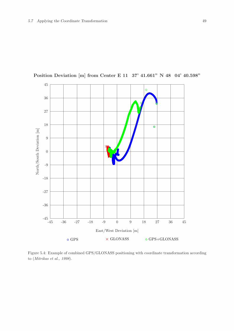
5.7 Applying the Coordinate Transformation 49
Position Deviation [m] from Center E 11� 37’ 41.661” N 48� 04’ 40.598”
◦ GPS × GLONASS ¦ GPS+GLONASS
East/West Deviation [m]
-45 -36 -27 -18 -9 0 9 18 27 36 45
Nor
th/S
outh
Dev
iati
on[m
]
-45
-36
-27
-18
-9
0
9
18
27
36
45
◦
◦◦◦◦◦◦◦◦◦◦◦◦◦◦◦◦◦◦◦◦◦◦◦◦
◦◦◦◦◦◦◦◦◦◦◦◦◦◦◦◦◦◦◦◦◦◦◦◦◦◦◦◦◦◦◦◦◦◦◦◦◦◦◦◦◦◦◦◦◦◦◦◦◦◦◦◦◦◦◦◦◦◦◦◦◦◦◦◦◦◦◦◦◦◦◦◦◦◦◦◦◦◦◦◦◦◦◦◦◦◦◦◦◦◦◦◦◦◦◦◦◦◦◦◦◦◦◦◦◦◦◦◦◦◦◦◦◦◦◦◦◦◦◦◦◦◦◦◦◦◦◦◦◦◦◦◦◦◦◦◦◦◦◦◦◦◦◦◦◦◦◦◦◦◦◦◦◦◦◦◦◦◦◦◦◦◦◦◦◦◦◦◦◦◦◦◦◦◦◦◦◦◦◦◦◦◦◦◦◦◦◦◦◦◦◦◦◦◦◦◦◦◦◦◦◦◦◦◦◦◦◦◦◦◦◦◦◦◦◦◦◦◦◦◦◦◦◦◦◦◦◦◦◦◦◦◦◦◦◦◦◦◦◦◦◦◦◦◦◦◦◦◦◦◦◦◦◦◦◦◦◦◦◦◦◦◦◦◦◦◦◦◦◦◦◦◦◦◦◦◦◦◦◦◦◦◦◦◦◦◦◦◦◦◦◦◦◦◦◦◦◦◦◦◦◦◦◦◦◦◦◦◦◦◦◦◦◦◦◦◦◦◦◦◦◦◦◦◦◦◦◦◦◦◦◦◦◦◦◦◦◦◦◦◦◦◦◦◦◦◦◦◦◦◦◦◦◦◦◦◦◦◦◦◦◦◦◦◦◦◦◦◦◦◦◦◦◦◦◦◦◦◦◦◦◦◦◦◦◦◦◦◦◦◦◦◦◦◦◦◦◦◦◦◦◦◦◦◦◦◦◦◦◦◦◦◦◦◦◦◦◦◦◦◦◦◦◦◦◦◦◦◦◦◦◦◦◦◦◦◦◦◦◦◦◦◦◦◦◦◦◦◦◦◦◦◦◦◦◦◦◦◦◦◦◦◦◦◦◦◦◦◦◦◦◦◦◦◦◦◦◦◦◦◦◦◦◦◦◦◦◦◦◦◦◦◦◦◦◦◦◦◦◦◦◦◦◦◦◦◦◦◦
◦◦◦◦◦◦◦◦◦◦◦◦◦◦◦◦◦◦◦◦◦◦◦◦◦◦◦◦◦◦◦◦◦◦◦◦◦◦◦◦◦◦◦◦◦◦◦◦◦◦◦◦◦◦◦◦◦◦◦◦◦◦◦◦◦◦◦◦◦◦◦◦◦◦◦◦◦◦◦◦◦◦◦◦◦◦◦◦◦◦◦◦◦◦◦◦◦◦◦◦◦◦◦◦◦◦◦◦◦◦◦◦◦◦◦◦◦◦◦◦◦◦◦◦◦◦◦◦◦◦◦◦◦◦◦◦◦◦◦◦◦◦◦◦◦◦◦◦◦◦◦◦◦◦◦◦◦◦◦◦◦◦◦◦◦◦◦◦◦◦◦◦◦◦◦◦◦◦◦◦◦◦◦◦◦◦◦◦◦◦◦◦◦◦◦◦◦◦◦◦◦◦◦◦◦◦◦◦◦◦◦◦◦◦◦◦◦◦◦◦◦◦◦◦◦◦◦◦◦◦◦◦◦◦◦◦◦◦◦◦◦◦◦◦◦◦◦◦◦◦◦◦◦◦◦◦◦◦◦◦◦◦◦◦◦◦◦◦◦◦◦◦◦◦◦◦◦◦◦◦◦◦◦◦◦◦◦◦◦◦◦◦◦◦◦◦◦◦◦◦◦◦◦◦◦◦◦◦◦◦◦◦◦◦◦◦◦◦◦◦◦◦◦◦◦◦◦◦◦◦◦◦◦◦◦◦◦◦◦◦◦◦◦◦◦◦◦◦◦◦◦◦◦◦◦◦◦◦◦◦◦◦◦◦◦◦◦◦◦◦◦◦◦◦◦◦◦◦◦◦◦◦◦◦◦◦◦◦◦◦◦◦◦◦◦◦◦◦◦◦◦◦◦◦◦◦◦◦◦◦◦◦◦◦◦◦◦◦◦◦◦◦◦◦◦◦◦◦◦◦◦◦◦◦◦◦◦◦◦◦◦◦◦◦◦◦◦◦◦◦◦◦◦◦◦◦◦◦◦◦◦◦◦◦◦◦◦◦◦◦◦◦◦◦◦◦◦◦◦◦◦◦◦◦◦◦◦◦◦◦◦◦◦◦◦◦◦◦◦◦◦◦◦◦◦◦◦◦◦◦◦◦◦◦◦◦◦◦◦◦◦◦◦◦◦◦◦◦◦◦◦◦◦◦◦◦◦◦◦◦◦◦◦◦◦◦◦◦◦◦◦◦◦◦◦◦◦◦◦◦◦◦◦◦◦◦◦◦◦◦◦◦◦◦◦◦◦◦◦◦◦◦◦◦◦◦◦◦◦◦◦◦◦◦◦◦◦◦◦◦◦◦◦◦◦◦◦◦◦◦◦◦◦◦◦◦◦◦◦◦◦◦◦◦◦◦◦◦◦◦◦◦◦◦◦◦◦◦◦◦◦◦◦◦◦◦◦◦◦◦◦◦◦◦◦◦◦◦◦◦◦◦◦◦◦◦◦◦◦◦◦◦◦◦◦◦◦◦◦◦◦◦◦◦◦◦◦◦◦◦◦◦◦◦◦◦◦◦◦◦◦◦◦◦◦◦◦◦◦◦◦◦◦◦◦◦◦◦◦◦◦◦◦◦◦◦◦◦◦◦◦◦◦◦◦◦◦◦◦◦◦◦◦◦◦◦◦◦◦◦◦◦◦◦◦◦◦◦◦◦◦◦◦◦◦◦◦◦◦◦◦◦◦◦◦◦◦◦◦◦◦◦◦◦◦◦◦◦◦◦◦◦◦◦◦◦◦◦◦◦◦◦◦◦◦◦◦◦◦◦◦◦◦◦◦◦◦◦◦◦◦◦◦◦◦◦◦◦◦◦◦◦◦◦◦◦◦◦◦◦◦◦◦◦◦◦◦◦◦◦◦◦◦◦◦◦◦◦◦◦◦◦◦◦◦◦◦◦◦◦◦◦◦◦◦◦◦◦◦◦◦◦◦◦◦◦◦◦◦◦◦◦◦◦◦◦◦◦◦◦◦◦◦◦◦◦◦◦◦◦◦◦◦◦◦◦◦◦◦◦◦◦◦◦◦◦◦◦◦◦◦◦◦◦◦◦◦◦◦◦◦◦◦◦◦◦◦◦◦◦◦◦◦◦◦◦◦◦◦◦◦◦◦◦◦◦◦◦◦◦◦◦◦◦◦◦◦◦◦◦◦◦◦◦◦◦◦◦◦◦◦◦◦◦◦◦◦◦◦◦◦◦◦◦◦◦◦◦◦◦◦◦◦◦◦◦◦◦◦◦◦◦◦◦◦◦◦◦◦◦◦◦◦◦◦◦◦◦◦◦◦◦◦◦◦◦◦◦◦◦◦◦◦◦◦◦◦◦◦◦◦◦◦◦◦◦◦◦◦◦◦◦◦◦◦◦◦◦◦◦◦◦◦◦◦◦◦◦◦◦◦◦◦◦◦◦◦◦◦◦◦◦◦◦◦◦◦◦◦◦◦◦◦◦◦◦◦◦◦◦◦◦◦◦◦◦◦◦◦◦◦◦◦◦◦◦◦◦◦◦◦◦◦◦◦◦◦◦◦◦◦◦◦◦◦◦◦◦◦◦◦◦◦◦◦◦◦◦◦◦◦◦◦◦◦◦◦◦◦◦◦◦◦◦◦◦◦◦◦◦◦◦◦◦◦◦◦◦◦◦◦◦◦◦◦◦◦◦◦◦◦◦◦◦◦◦◦◦◦◦◦◦◦◦◦◦◦◦◦◦◦◦◦◦◦◦◦◦◦◦
◦◦◦◦◦◦◦◦◦◦◦◦◦◦◦◦◦◦◦◦◦◦◦◦◦◦◦◦◦◦◦◦◦◦◦◦◦◦◦◦◦◦◦◦◦◦◦◦◦◦◦◦◦◦◦◦◦◦◦◦◦◦◦◦◦◦◦◦◦◦◦◦◦◦◦◦◦◦◦◦◦◦◦◦◦◦◦◦◦◦◦◦◦◦◦◦◦◦◦◦◦◦◦◦◦◦◦◦◦◦◦◦◦◦◦◦◦◦◦◦◦◦◦◦◦◦◦◦◦◦◦◦◦◦◦◦◦◦◦◦◦◦◦◦◦◦◦◦◦◦◦◦◦◦◦◦◦◦◦◦◦◦◦◦◦◦◦◦◦◦◦◦◦◦◦◦◦◦◦◦◦◦◦◦◦◦◦◦◦◦◦◦◦◦◦◦◦◦◦◦◦◦◦◦◦◦◦◦◦◦◦◦◦◦◦◦◦◦◦◦◦◦◦◦◦◦◦◦◦◦◦◦◦◦◦◦◦◦◦◦◦◦◦◦◦◦◦◦◦◦◦◦◦◦◦◦◦◦◦◦◦◦◦◦◦◦◦◦◦◦◦◦◦◦◦◦◦◦◦◦◦◦◦◦◦◦◦◦◦◦◦◦◦◦◦◦◦◦◦◦◦◦◦◦◦◦◦◦◦◦◦◦◦◦◦◦◦◦◦◦◦◦◦◦◦◦◦◦◦◦◦◦◦◦◦◦◦◦◦◦◦◦◦◦◦◦◦◦◦◦◦◦◦◦◦◦◦◦◦◦◦◦◦◦◦◦◦◦◦◦◦◦◦◦◦◦◦◦◦◦◦◦◦◦◦◦◦◦◦◦◦◦◦◦◦◦◦◦◦◦◦◦◦◦◦◦◦◦◦◦◦◦◦◦◦◦◦◦◦◦◦◦◦◦◦◦◦◦◦◦◦◦◦◦◦◦◦◦◦◦◦◦◦◦◦◦◦◦◦◦◦◦◦◦◦◦◦◦◦◦◦◦◦◦◦◦◦◦◦◦◦◦◦◦◦◦◦◦◦◦◦◦◦◦◦◦◦◦◦◦◦◦◦◦◦◦◦◦◦◦◦◦◦◦◦◦◦◦◦◦◦◦◦◦◦◦◦◦◦◦◦◦◦◦◦◦◦◦◦◦◦◦◦◦◦◦◦◦◦◦◦◦◦◦◦◦◦◦◦◦◦◦◦◦◦◦◦◦◦◦◦◦◦◦◦◦◦◦◦◦◦◦◦◦◦◦◦◦◦◦◦◦◦◦◦◦◦◦◦◦◦◦◦◦◦◦◦◦◦◦◦◦◦◦◦◦◦◦◦◦◦◦◦◦◦◦◦◦◦◦◦◦◦◦◦◦◦◦◦◦◦◦◦◦◦◦◦◦◦◦◦◦◦◦◦◦◦◦◦◦◦◦◦◦◦◦◦◦◦◦◦◦◦◦◦◦◦◦◦◦◦◦◦◦◦◦◦◦◦◦◦◦◦◦◦◦◦◦◦◦◦◦◦◦◦◦◦◦◦◦◦◦◦◦◦◦◦◦◦◦◦◦◦◦◦◦◦◦◦◦◦◦◦◦◦◦◦◦◦◦◦◦◦◦◦◦◦◦◦◦◦◦◦◦◦◦◦◦◦◦◦◦◦◦◦◦◦◦◦◦◦◦◦◦◦◦◦◦◦◦◦◦◦◦◦◦◦◦◦◦◦◦◦◦◦◦◦◦◦◦◦◦◦◦◦◦◦◦◦◦◦◦◦◦◦◦◦◦◦◦◦◦◦◦◦◦◦◦◦◦◦◦◦◦◦◦◦◦◦◦◦◦◦◦◦◦◦◦◦◦◦◦◦◦◦◦◦◦◦◦◦◦◦◦◦◦◦◦◦◦◦◦◦◦◦◦◦◦◦◦◦◦◦◦◦◦◦◦◦◦◦◦◦◦◦◦◦◦◦◦◦◦◦◦◦◦◦◦◦◦◦◦◦◦◦◦◦◦◦◦◦◦◦◦◦◦◦◦◦◦◦◦◦◦◦◦◦◦◦◦◦◦◦◦◦◦◦◦◦◦◦◦◦◦◦◦◦◦◦◦◦◦◦◦◦◦◦◦◦◦◦◦◦◦◦◦◦◦◦◦◦◦◦◦◦◦◦◦◦◦◦◦◦◦◦◦◦◦◦◦◦◦◦◦◦◦◦◦◦◦◦◦◦◦◦◦◦◦◦◦◦◦◦◦◦◦◦◦◦◦◦◦◦◦◦◦◦◦◦◦◦◦◦◦◦◦◦◦◦◦◦◦◦◦◦◦◦◦◦◦◦◦◦◦◦◦◦◦◦◦◦◦◦◦◦◦◦◦◦◦◦◦◦◦◦◦◦◦◦◦◦◦◦◦◦◦◦◦◦◦◦◦◦◦◦◦◦◦◦◦◦◦◦◦◦◦◦◦◦◦◦◦◦◦◦◦◦◦◦◦◦◦◦◦◦◦◦◦◦◦◦◦◦◦◦◦◦◦◦◦◦◦◦◦◦◦◦◦◦◦◦◦◦◦◦◦◦◦◦◦◦◦◦◦◦◦◦◦◦◦◦◦◦◦◦◦◦◦◦◦◦◦◦◦◦◦◦◦◦◦◦◦◦◦◦◦◦◦◦◦◦◦◦◦◦◦◦◦◦◦◦◦◦◦◦◦◦◦◦◦◦◦◦◦◦◦◦◦◦◦◦◦◦◦◦◦◦◦◦◦◦◦◦◦◦◦◦◦◦◦◦◦◦◦◦◦◦◦◦◦◦◦◦◦◦◦◦◦◦◦◦◦◦◦◦◦◦◦◦◦◦◦◦◦◦◦◦◦◦◦◦◦◦◦◦◦◦◦◦◦◦◦◦◦◦◦◦◦◦◦◦◦◦◦◦◦◦◦◦◦◦◦◦◦◦◦◦◦◦◦◦◦◦◦◦◦◦◦◦◦◦◦◦◦◦◦◦◦◦◦◦◦◦◦◦◦◦◦◦◦◦◦◦◦◦◦◦◦◦◦◦◦◦◦◦◦◦◦◦◦◦◦◦◦◦◦◦◦◦◦◦◦◦◦◦◦◦◦◦◦◦◦◦◦◦◦◦◦◦◦◦◦◦◦◦◦◦◦◦◦◦◦◦◦◦◦◦◦◦◦◦◦◦◦◦◦◦◦◦
××××××××××××××××××××××××××××××××××××××××××××××××××××××××××××××××××××××××××××××××××××××××××××××××××××××××××××××××××××××××××××××××××××××××××××××××××××××××××××××××××××××××××××××××××××××××××××××××××××××××××××××××××××××××××××××××××××××××××××××××××××××××××××××××××××××××××××××××××××××××××××××××××××××××××××××××××××××××××××××××××××××××××××××××××××××××××××××××××××××××××××××××××××××××××××××××××××××××××××××××××××××××××××××××××××××××××××××××××××××××××××××××××××××××××××××××××××××××××××××××××××××××××××××××××××××××××××××××××××××××××××××××××××××××××××××××××××××××××××××××××××××××××××××××××××××××××××××××××××××××××××××××××××××××××××××××××××××××××××××××××××××××××××××××××××××××××××××××××××××××××××××××××××××××××××××××××××××××××××××××××××××××××××××××××××××××××××××××××××××××××××××××××××××××××××××××××××××××××××××××××××××××××××
¦
¦
¦
¦¦¦¦¦¦¦¦¦¦¦¦¦¦¦¦¦¦¦¦¦¦¦¦¦¦¦
¦¦¦¦¦¦¦¦¦¦¦¦¦¦¦¦¦¦¦¦¦¦¦¦¦¦¦¦¦¦¦¦¦¦¦¦¦¦¦¦¦¦¦¦¦¦¦¦¦¦¦¦¦¦¦¦¦¦¦¦¦¦¦¦¦¦¦¦¦¦¦¦¦¦¦¦¦¦¦¦¦¦¦¦¦¦¦¦¦¦¦¦¦¦¦¦¦¦¦¦¦¦¦¦¦¦¦¦¦¦¦¦¦¦¦¦¦¦¦¦¦¦¦¦¦¦¦¦¦¦¦¦¦¦¦¦¦¦¦¦¦¦¦¦¦¦¦¦¦¦¦¦¦¦¦¦¦¦¦¦¦¦¦¦¦¦¦¦¦¦¦¦¦¦¦¦¦¦¦¦¦¦¦¦¦¦¦¦¦¦¦¦¦¦¦¦¦¦¦¦¦¦¦¦¦¦¦¦¦¦¦¦¦¦¦¦¦¦¦¦¦¦¦¦¦¦¦¦¦¦¦¦¦¦¦¦¦¦¦¦¦¦¦¦¦¦¦¦¦¦¦¦¦¦¦¦¦¦¦¦¦¦¦¦¦¦¦¦¦¦¦¦¦¦¦¦¦¦¦¦¦¦¦¦¦¦¦¦¦¦¦¦¦¦¦¦¦¦¦¦¦¦¦¦¦¦¦¦¦¦¦¦¦¦¦¦¦¦¦¦¦¦¦¦¦¦¦¦¦¦¦¦¦¦¦¦¦¦¦¦¦¦¦¦¦¦¦¦¦¦¦¦¦¦¦¦¦¦¦¦¦¦¦¦¦¦¦¦¦¦¦¦¦¦¦¦¦¦¦¦¦¦¦¦¦¦¦¦¦¦¦¦¦¦¦¦¦¦¦¦¦¦¦¦¦¦¦¦¦¦¦¦¦¦¦¦¦¦¦¦¦¦¦¦¦¦¦¦¦¦¦¦¦¦¦¦¦¦¦¦¦¦¦¦¦¦¦¦¦¦¦¦¦¦¦¦¦¦¦¦¦¦¦¦¦¦¦¦¦¦¦¦¦¦¦¦¦¦¦¦¦¦¦¦¦¦¦¦¦¦¦¦¦¦¦¦¦¦¦¦¦¦¦¦¦¦¦¦¦¦¦¦¦¦¦¦¦¦¦¦¦¦¦¦¦¦¦¦¦¦¦¦¦¦¦¦¦¦¦¦¦¦¦¦¦¦¦¦¦¦¦¦¦¦¦¦¦¦¦¦¦¦¦¦¦¦¦¦¦¦¦¦¦¦¦¦¦¦¦¦¦¦¦¦¦¦¦¦¦¦¦¦¦¦¦¦¦¦¦¦¦¦¦¦¦¦¦¦¦¦¦¦¦¦¦¦¦¦¦¦¦¦¦¦¦¦¦¦¦¦¦¦¦¦¦¦¦¦¦¦¦¦¦¦¦¦¦¦¦¦¦¦¦¦¦¦¦¦¦¦¦¦¦¦¦¦¦¦¦¦¦¦¦¦¦¦¦¦¦¦¦¦¦¦¦¦¦¦¦¦¦¦¦¦¦¦¦¦¦¦¦¦¦¦¦¦¦¦¦¦¦¦¦¦¦¦¦¦¦¦¦¦¦¦¦¦¦¦¦¦¦¦¦¦¦¦¦¦¦¦¦¦¦¦¦¦¦¦¦¦¦¦¦¦¦¦¦¦¦¦¦¦¦¦¦¦¦¦¦¦¦¦¦¦¦¦¦¦¦¦¦¦¦¦¦¦¦¦¦¦¦¦¦¦¦¦¦¦¦¦¦¦¦¦¦¦¦¦¦¦¦¦¦¦¦¦¦¦¦¦¦¦¦¦¦¦¦¦¦¦¦¦¦¦¦¦¦¦¦¦¦¦¦¦¦¦¦¦¦¦¦¦¦¦¦¦¦¦¦¦¦¦¦¦¦¦¦¦¦¦¦¦¦¦¦¦¦¦¦¦¦¦¦¦¦¦¦¦¦¦¦¦¦¦¦¦¦¦¦¦¦¦¦¦¦¦¦¦¦¦¦¦¦¦¦¦¦¦¦¦¦¦¦¦¦¦¦¦¦¦¦¦¦¦¦¦¦¦¦¦¦¦¦¦¦¦¦¦¦¦¦¦¦¦¦¦¦¦¦¦¦¦¦¦¦¦¦¦¦¦¦¦¦¦¦¦¦¦¦¦¦¦¦¦¦¦¦¦¦¦¦¦¦¦¦¦¦¦¦¦¦¦¦¦¦¦¦¦¦¦¦¦¦¦¦¦¦¦¦¦¦¦¦¦¦¦¦¦¦¦¦¦¦¦¦¦¦¦¦¦¦¦¦¦¦¦¦¦¦¦¦¦¦¦¦¦¦¦¦¦¦¦¦¦¦¦¦¦¦¦¦¦¦¦¦¦¦¦¦¦¦¦¦¦¦¦¦¦¦¦¦¦¦¦¦¦¦¦¦¦¦¦¦¦¦¦¦¦¦¦¦¦¦¦¦¦¦¦¦¦¦¦¦¦¦¦¦¦¦¦¦¦¦¦¦¦¦¦¦¦¦¦¦¦¦¦¦¦¦¦¦¦¦¦¦¦¦¦¦¦¦¦¦¦¦¦¦¦¦¦¦¦¦¦¦¦¦¦¦¦¦¦¦¦¦¦¦¦¦¦¦¦¦¦¦¦¦¦¦¦¦¦¦¦¦¦¦¦¦¦¦¦¦¦¦¦¦¦¦¦¦¦¦¦¦¦¦¦¦¦¦¦¦¦¦¦¦¦¦¦¦¦¦¦¦¦¦¦¦¦¦¦¦¦¦¦¦¦¦¦¦¦¦¦¦¦¦¦¦¦¦¦¦¦¦¦¦¦¦¦¦¦¦¦¦¦¦¦¦¦¦¦¦¦¦¦¦¦¦¦¦¦¦¦¦¦¦¦¦¦¦¦¦¦¦¦¦¦¦¦¦¦¦¦¦¦¦¦¦¦¦¦¦¦¦¦¦¦¦¦¦¦¦¦¦¦¦¦¦¦¦¦¦¦¦¦¦¦¦¦¦¦¦¦¦¦¦¦¦¦¦¦¦¦¦¦¦¦¦¦¦¦¦¦¦¦¦¦¦¦¦¦¦¦¦¦¦¦¦¦¦¦¦¦¦¦¦¦¦¦¦¦¦¦¦¦¦¦¦¦¦¦¦¦¦¦¦¦¦¦¦¦¦¦¦¦¦¦¦¦¦¦¦¦¦¦¦¦¦¦¦¦¦¦¦¦¦¦¦¦¦¦¦¦¦¦¦¦¦¦¦¦¦¦¦¦¦¦¦¦¦¦¦¦¦¦¦¦¦¦¦¦¦¦¦¦¦¦¦¦¦¦¦¦¦¦¦¦¦¦¦¦¦¦¦¦¦¦¦¦¦¦¦¦¦¦¦¦¦¦¦¦¦¦¦¦¦¦¦¦¦¦¦¦¦¦¦¦¦¦¦¦¦¦¦¦¦¦¦¦¦¦¦¦¦¦¦¦¦¦¦¦¦¦¦¦¦¦¦¦¦¦¦¦¦¦¦¦¦¦¦¦¦¦¦¦¦¦¦¦¦¦¦¦¦¦¦¦¦¦¦¦¦¦¦¦¦¦¦¦¦¦¦¦¦¦¦¦¦¦¦¦¦¦¦¦¦¦¦¦¦¦¦¦¦¦¦¦¦¦¦¦¦¦¦¦¦¦¦¦¦¦¦¦¦¦¦¦¦¦¦¦¦¦¦¦¦¦¦¦¦¦¦¦¦¦¦¦¦¦¦¦¦¦¦¦¦¦¦¦¦¦¦¦¦¦¦¦¦¦¦¦¦¦¦¦¦¦¦¦¦¦¦¦¦¦¦¦¦¦¦¦¦¦¦¦¦¦¦¦¦¦¦¦¦¦¦¦¦
¦¦¦¦¦¦¦¦¦¦¦¦¦¦¦¦¦¦¦¦¦¦¦¦¦¦¦¦¦¦¦¦¦¦¦¦¦¦¦¦¦¦¦¦¦¦¦¦¦¦¦¦¦¦¦¦¦¦¦¦¦¦¦¦¦¦¦¦¦¦¦¦¦¦¦¦¦¦¦¦¦¦¦¦¦¦¦¦¦¦¦¦¦¦¦¦¦¦¦¦¦¦¦¦¦¦¦¦¦¦¦¦¦¦¦¦¦¦¦¦¦¦¦¦¦¦¦¦¦¦¦¦¦¦¦¦¦¦¦¦¦¦¦¦¦¦¦¦¦¦¦¦¦¦¦¦¦¦¦¦¦¦¦¦¦¦¦¦¦¦¦¦¦¦¦¦¦¦¦¦¦¦¦¦¦¦¦¦¦¦¦¦¦¦¦¦¦¦¦¦¦¦¦¦¦¦¦¦¦¦¦¦¦¦¦¦¦¦¦¦¦¦¦¦¦¦¦¦¦¦¦¦¦¦¦¦¦¦¦¦¦¦¦¦¦¦¦¦¦¦¦¦¦¦¦¦¦¦¦¦¦¦¦¦¦¦¦¦¦¦¦¦¦¦¦¦¦¦¦¦¦¦¦¦¦¦¦¦¦¦¦¦¦¦¦¦¦¦¦¦¦¦¦¦¦¦¦¦¦¦¦¦¦¦¦¦¦¦¦¦¦¦¦¦¦¦¦¦¦¦¦¦¦¦¦¦¦¦¦¦¦¦¦¦¦¦¦¦¦¦¦¦¦¦¦¦¦¦¦¦¦¦¦¦¦¦¦¦¦¦¦¦¦¦¦¦¦¦¦¦¦¦¦¦¦¦¦¦¦¦¦¦¦¦¦¦¦¦¦¦¦¦¦¦¦¦¦¦¦¦¦¦¦¦¦¦¦¦¦¦¦¦¦¦¦¦¦¦¦¦¦¦¦¦¦¦¦¦¦¦¦¦¦¦¦¦¦¦¦¦¦¦¦¦¦¦¦¦¦¦¦¦¦¦¦¦¦¦¦¦¦¦¦¦¦¦¦¦¦¦¦¦¦¦¦¦¦¦¦¦¦¦¦¦¦¦¦¦¦¦¦¦¦¦¦¦¦¦¦¦¦¦¦¦¦¦¦¦¦¦¦¦¦¦¦¦¦¦¦¦¦¦¦¦¦¦¦¦¦¦¦¦¦¦¦¦¦¦¦¦¦¦¦¦¦¦¦¦¦¦¦¦¦¦¦¦¦¦¦¦¦¦¦¦¦¦¦¦¦¦¦¦¦¦¦¦¦¦¦¦¦¦¦¦¦¦¦¦¦¦¦¦¦¦¦¦¦¦¦¦¦¦¦¦¦¦¦¦¦¦¦¦¦¦¦¦¦¦¦¦¦¦¦¦¦¦¦¦¦¦¦¦¦¦¦¦¦¦¦¦¦¦¦¦¦¦¦¦¦¦¦¦¦¦¦¦¦¦¦¦¦¦¦¦¦¦¦¦¦¦¦¦¦¦¦¦¦¦¦¦¦¦¦¦¦¦¦¦¦¦¦¦¦¦¦¦¦¦¦¦¦¦¦¦¦¦¦¦¦¦¦¦¦¦¦¦¦¦¦¦¦¦¦¦¦¦¦¦¦¦¦¦¦¦¦¦¦¦¦¦¦¦¦¦¦¦¦¦¦¦¦¦¦¦¦¦¦¦¦¦¦¦¦¦¦¦¦¦¦¦¦¦¦¦¦¦¦¦¦¦¦¦¦¦¦¦¦¦¦¦¦¦¦¦¦¦¦¦¦¦¦¦¦¦¦¦¦¦¦¦¦¦¦¦¦¦¦¦¦¦¦¦¦¦¦¦¦¦¦¦¦¦¦¦¦¦¦¦¦¦¦¦¦¦¦¦¦¦¦¦¦¦¦¦¦¦¦¦¦¦¦¦¦¦¦¦¦¦¦¦¦¦¦¦¦¦¦¦¦¦¦¦¦¦¦¦¦¦¦¦¦¦¦¦¦¦¦¦¦¦¦¦¦¦¦¦¦¦¦¦¦¦¦¦¦¦¦¦¦¦¦¦¦¦¦¦
Figure 5.4: Example of combined GPS/GLONASS positioning with coordinate transformation accordingto (Mitrikas et al., 1998).
50 5 COORDINATE SYSTEMS
5.8 Coordinate Frames in Differential Processing
Where better accuracy is required, e.g. in surveying and geodesy, positioning will usually be done indifferential mode. In this case, differences in the coordinate frame of the satellite positions can beregarded as orbital errors, which cancel out in differential processing, at least over short baselines.
According to (Beutler et al., 1987; Landau and Vollath, 1996), a radial error of 4 m will lead to anerror of approximately 0.03 ppm in the baseline. Orbital errors of 75 m along track or cross track (whichwould correspond to the coordinate transformation (Misra and Abbot, 1994)) may cause a rotation of thebaseline of around 0.6” and a maximum baseline error of 2.8 ppm.
Writing a simplified pseudorange observation equation from receiver R to satellite S, considering theerror in orbit determination eorb:
PRSR = %S
R + c · δtR − c · δtS + eS,orbR (5.8.1)
and linearizing this equation with
%SR =
√(xR − xS)2 + (yR − yS)2 + (zR − zS)2 (5.8.2)
the position vectors of receiver ~xR and satellite ~xS must be given in the same coordinate frame.In case the satellite position vector is given in a different coordinate frame ~xS with a locally valid
transformation ~xS = ~xS + δ~x, Eq. (5.8.1) rewrites to
PRSR =
√(xR − xS − δx)2 + (yR − yS − δy)2 + (zR − zS − δz)2 + c · δtR − c · δtS + eS,orb
R (5.8.3)
Linearizing the geometric range in terms of components of the transformation around zero:
%SR(δx, δy, δz) = %S
R(δx = 0, δy = 0, δz = 0) +∂%S
R(δx, δy, δz)∂δx
∣∣∣∣ δx = 0δy = 0δz = 0
· δx + (5.8.4)
∂%SR(δx, δy, δz)
∂δy
∣∣∣∣ δx = 0δy = 0δz = 0
· δy +∂%S
R(δx, δy, δz)∂δz
∣∣∣∣ δx = 0δy = 0δz = 0
· δz
= %SR −
xR − xS
%SR
· δx− yR − yS
%SR
· δy − zR − zS
%SR
· δz (5.8.5)
= %SR + f(~xR, ~xS , δ~x) (5.8.6)
with the range in different coordinate frames
%SR =
√(xR − xS)2 + (yR − yS)2 + (zR − zS)2 (5.8.7)
Thus, we can write for the pseudorange observation equation
PRSR = %S
R + f(~xR, ~xS , δ~x) + c · δtR − c · δtS + eS,orbR (5.8.8)
Doing the same for a second user receiver U :
PRSU = %S
U + f(~xU , ~xS , δ~x) + c · δtU − c · δtS + eS,orbU (5.8.9)
and forming the receiver-to-receiver single difference, we obtain:
∆PRSUR = ∆%S
UR + c ·∆δtUR + f(~xU , ~xS , δ~x)− f(~xR, ~xS , δ~x) + ∆eS,orbUR (5.8.10)
For short baselines between user and reference receivers, the orbital errors will be very similar:∆eS,orb
UR → 0 for ~xU → ~xR.
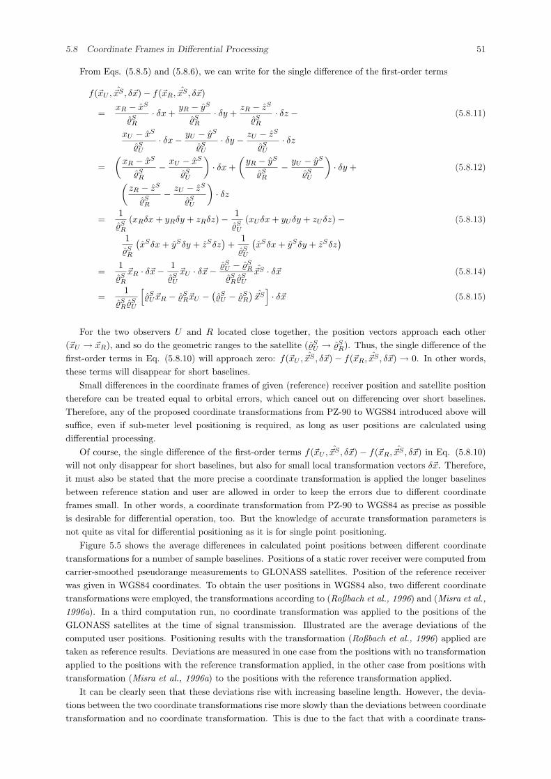
5.8 Coordinate Frames in Differential Processing 51
From Eqs. (5.8.5) and (5.8.6), we can write for the single difference of the first-order terms
f(~xU , ~xS , δ~x)− f(~xR, ~xS , δ~x)
=xR − xS
%SR
· δx +yR − yS
%SR
· δy +zR − zS
%SR
· δz − (5.8.11)
xU − xS
%SU
· δx− yU − yS
%SU
· δy − zU − zS
%SU
· δz
=(
xR − xS
%SR
− xU − xS
%SU
)· δx +
(yR − yS
%SR
− yU − yS
%SU
)· δy + (5.8.12)
(zR − zS
%SR
− zU − zS
%SU
)· δz
=1
%SR
(xRδx + yRδy + zRδz)− 1%S
U
(xUδx + yUδy + zUδz)− (5.8.13)
1%S
R
(xSδx + ySδy + zSδz
)+
1%S
U
(xSδx + ySδy + zSδz
)
=1
%SR
~xR · δ~x− 1%S
U
~xU · δ~x− %SU − %S
R
%SR%S
U
~xS · δ~x (5.8.14)
=1
%SR%S
U
[%S
U~xR − %SR~xU −
(%S
U − %SR
)~xS
]· δ~x (5.8.15)
For the two observers U and R located close together, the position vectors approach each other(~xU → ~xR), and so do the geometric ranges to the satellite (%S
U → %SR). Thus, the single difference of the
first-order terms in Eq. (5.8.10) will approach zero: f(~xU , ~xS , δ~x) − f(~xR, ~xS , δ~x) → 0. In other words,these terms will disappear for short baselines.
Small differences in the coordinate frames of given (reference) receiver position and satellite positiontherefore can be treated equal to orbital errors, which cancel out on differencing over short baselines.Therefore, any of the proposed coordinate transformations from PZ-90 to WGS84 introduced above willsuffice, even if sub-meter level positioning is required, as long as user positions are calculated usingdifferential processing.
Of course, the single difference of the first-order terms f(~xU , ~xS , δ~x) − f(~xR, ~xS , δ~x) in Eq. (5.8.10)will not only disappear for short baselines, but also for small local transformation vectors δ~x. Therefore,it must also be stated that the more precise a coordinate transformation is applied the longer baselinesbetween reference station and user are allowed in order to keep the errors due to different coordinateframes small. In other words, a coordinate transformation from PZ-90 to WGS84 as precise as possibleis desirable for differential operation, too. But the knowledge of accurate transformation parameters isnot quite as vital for differential positioning as it is for single point positioning.
Figure 5.5 shows the average differences in calculated point positions between different coordinatetransformations for a number of sample baselines. Positions of a static rover receiver were computed fromcarrier-smoothed pseudorange measurements to GLONASS satellites. Position of the reference receiverwas given in WGS84 coordinates. To obtain the user positions in WGS84 also, two different coordinatetransformations were employed, the transformations according to (Roßbach et al., 1996) and (Misra et al.,1996a). In a third computation run, no coordinate transformation was applied to the positions of theGLONASS satellites at the time of signal transmission. Illustrated are the average deviations of thecomputed user positions. Positioning results with the transformation (Roßbach et al., 1996) applied aretaken as reference results. Deviations are measured in one case from the positions with no transformationapplied to the positions with the reference transformation applied, in the other case from positions withtransformation (Misra et al., 1996a) to the positions with the reference transformation applied.
It can be clearly seen that these deviations rise with increasing baseline length. However, the devia-tions between the two coordinate transformations rise more slowly than the deviations between coordinatetransformation and no coordinate transformation. This is due to the fact that with a coordinate trans-
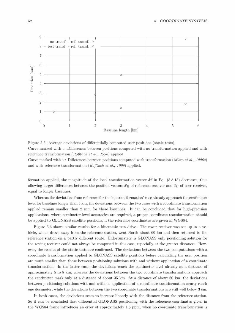
52 5 COORDINATE SYSTEMS
0
1
2
3
4
5
6
7
8
9
0 1 2 3 4 5 6
Dev
iati
on[m
m]
Baseline length [km]
no transf. - ref. transf.
◦
◦
◦
◦◦test transf. - ref. transf.
× ××
×
×
Figure 5.5: Average deviations of differentially computed user positions (static tests).Curve marked with ◦: Differences between positions computed with no transformation applied and withreference transformation (Roßbach et al., 1996) applied.Curve marked with ×: Differences between positions computed with transformation (Misra et al., 1996a)and with reference transformation (Roßbach et al., 1996) applied.
formation applied, the magnitude of the local transformation vector δ~x in Eq. (5.8.15) decreases, thusallowing larger differences between the position vectors ~xR of reference receiver and ~xU of user receiver,equal to longer baselines.
Whereas the deviations from reference for the ’no transformation’ case already approach the centimeterlevel for baselines longer than 5 km, the deviations between the two cases with a coordinate transformationapplied remain smaller than 2 mm for these baselines. It can be concluded that for high-precisionapplications, where centimeter-level accuracies are required, a proper coordinate transformation shouldbe applied to GLONASS satellite positions, if the reference coordinates are given in WGS84.
Figure 5.6 shows similar results for a kinematic test drive. The rover receiver was set up in a ve-hicle, which drove away from the reference station, went North about 60 km and then returned to thereference station on a partly different route. Unfortunately, a GLONASS only positioning solution forthe roving receiver could not always be computed in this case, especially at the greater distances. How-ever, the results of the static tests are confirmed. The deviations between the two computations with acoordinate transformation applied to GLONASS satellite positions before calculating the user positionare much smaller than those between positioning solutions with and without application of a coordinatetransformation. In the latter case, the deviations reach the centimeter level already at a distance ofapproximately 5 to 8 km, whereas the deviations between the two coordinate transformations approachthe centimeter mark only at a distance of about 35 km. At a distance of about 60 km, the deviationsbetween positioning solutions with and without application of a coordinate transformation nearly reachone decimeter, while the deviations between the two coordinate transformations are still well below 3 cm.
In both cases, the deviations seem to increase linearly with the distance from the reference station.So it can be concluded that differential GLONASS positioning with the reference coordinates given inthe WGS84 frame introduces an error of approximately 1.5 ppm, when no coordinate transformation is
5.9 GLONASS Ephemerides in WGS84 53
0
10
20
30
40
50
60
70
80
90
0 10 20 30 40 50 60 70
Dev
iati
on[m
m]
Distance [km]
no transf. - ref. transf.
◦ ◦◦◦◦◦◦◦◦ ◦◦◦◦◦◦◦◦◦
◦◦
◦◦◦◦◦◦◦◦◦◦◦◦◦◦◦◦
◦◦◦◦◦◦◦◦◦◦◦◦◦◦◦◦◦◦◦◦◦◦◦◦◦◦◦◦◦◦◦◦◦◦◦◦◦◦◦◦◦◦◦◦◦◦◦◦◦◦◦◦◦◦◦◦◦◦◦◦◦◦◦◦◦◦◦◦◦◦◦◦◦◦◦◦◦◦◦◦◦◦◦◦◦◦◦◦◦◦◦◦◦◦◦◦◦◦◦◦◦◦◦◦◦◦◦◦◦◦◦◦◦◦◦◦◦◦◦◦◦◦◦◦◦◦◦◦◦◦◦◦◦◦◦◦◦◦◦◦◦◦◦◦◦◦◦◦◦◦◦◦◦◦◦◦◦◦◦◦◦◦◦◦◦◦◦◦◦◦◦◦◦◦◦◦◦◦◦◦◦◦◦◦◦◦◦◦◦◦◦◦◦◦◦◦◦◦◦◦◦◦◦◦◦◦◦◦◦◦◦◦◦◦◦◦◦◦◦◦◦◦◦◦◦◦◦◦◦◦◦◦◦◦◦◦◦◦◦◦◦◦◦◦◦◦◦◦◦◦◦◦◦◦◦◦◦◦◦◦◦◦◦◦◦◦◦◦◦◦◦◦◦◦◦◦◦◦◦◦◦◦◦◦◦◦◦◦◦◦◦◦◦◦◦◦◦◦◦◦◦◦◦◦◦◦◦◦◦◦◦◦◦◦◦◦◦◦◦◦◦◦◦◦◦◦◦◦◦◦◦◦◦◦◦◦◦◦◦◦◦◦◦◦◦◦◦◦◦◦◦◦◦◦◦◦◦◦◦◦◦◦◦◦◦◦◦◦◦◦◦◦◦◦◦◦◦◦◦◦◦◦◦◦◦◦◦◦◦◦◦◦◦◦◦◦◦◦◦◦◦◦◦◦◦◦◦◦◦◦◦◦◦◦◦◦◦◦◦◦◦◦◦◦◦◦◦◦◦◦◦◦◦◦◦◦◦◦◦◦◦◦◦◦◦◦◦◦◦◦◦◦◦◦◦◦◦◦◦◦◦◦◦◦◦◦◦◦◦◦◦◦◦◦◦◦◦◦◦◦◦◦◦◦◦◦◦◦◦◦◦◦◦◦◦◦◦◦◦◦◦◦◦◦◦◦◦◦◦◦◦◦◦◦◦◦◦◦◦◦◦◦◦◦◦◦◦◦◦◦◦◦◦◦◦◦◦◦
◦test transf. - ref. transf.
××××××××× ×××××××××
×××××××××××××
×××××××××××××××××××××××××××××××××××××××××××××××××××××××××××××××××××××××××××××××××××××××××××××××××××××××××××××××××××××××××××××××××××××××××××××××××××××××××××××××××××××××××××××××××××××××××××××××××××××××××××××××××××××××××××××××××××××××××××××××××××××××××××××××××××××××××××××××××××××××××××××××××××××××××××××××××××××××××××××××××××××××××××××××××××××××××××××××××××××××××××××××××××××××××××××××××××××××××××××××××××××××××××××××××××××××××××××××××××××××××××××××××××××××××××××××××××××××××××××××××××××××××××××××××××××××××××××××××××××××××××××××××××××××××××××××
×
Figure 5.6: Deviations of differentially computed user positions (kinematic tests).Curve marked with ◦: Differences between positions computed with no transformation applied and withreference transformation (Roßbach et al., 1996) applied.Curve marked with ×: Differences between positions computed with transformation (Misra et al., 1996a)and with reference transformation (Roßbach et al., 1996) applied.
applied to the GLONASS satellite positions. With a proper coordinate transformation applied, theseerrors can be reduced considerably to around 0.5 ppm.
These were examples of GLONASS only processing. In combined GPS/GLONASS processing, thedeviations will be smaller, due to the influence of the GPS satellites, which do not require a coordinatetransformation. The exact amount will depend on how many GPS and GLONASS satellites contributeto the solution. But still, a proper coordinate transformation should be applied to GLONASS satellitepositions in order to keep errors caused by the different coordinate frames small.
In differential navigation, when meter-level accuracy is sufficient, doing without a coordinate trans-formation may not contribute significantly to the error level even for baselines of 50 km and more.
5.9 GLONASS Ephemerides in WGS84
Part of the data products of the IGEX-98 campaign were and still are precise ephemerides of GLO-NASS satellites, given in the WGS84 frame. When using these ephemeris data, the need for convertingGLONASS satellite coordinates from PZ-90 to WGS84 drops.
However, as with the precise GPS ephemerides, these data are not available in real-time. Therefore,these ephemerides can only be applied when post-processing observation data. They cannot be used inreal-time navigation.

54 5 COORDINATE SYSTEMS
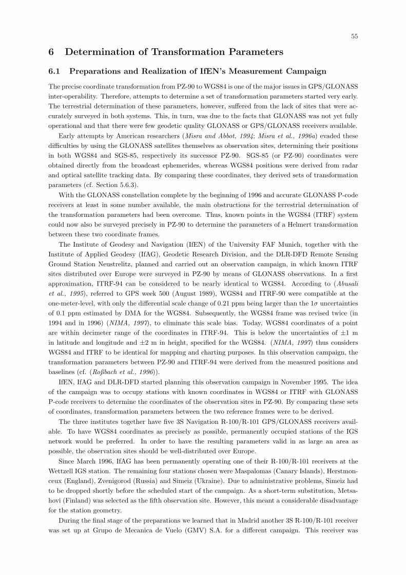
55
6 Determination of Transformation Parameters
6.1 Preparations and Realization of IfEN’s Measurement Campaign
The precise coordinate transformation from PZ-90 to WGS84 is one of the major issues in GPS/GLONASSinter-operability. Therefore, attempts to determine a set of transformation parameters started very early.The terrestrial determination of these parameters, however, suffered from the lack of sites that were ac-curately surveyed in both systems. This, in turn, was due to the facts that GLONASS was not yet fullyoperational and that there were few geodetic quality GLONASS or GPS/GLONASS receivers available.
Early attempts by American researchers (Misra and Abbot, 1994; Misra et al., 1996a) evaded thesedifficulties by using the GLONASS satellites themselves as observation sites, determining their positionsin both WGS84 and SGS-85, respectively its successor PZ-90. SGS-85 (or PZ-90) coordinates wereobtained directly from the broadcast ephemerides, whereas WGS84 positions were derived from radarand optical satellite tracking data. By comparing these coordinates, they derived sets of transformationparameters (cf. Section 5.6.3).
With the GLONASS constellation complete by the beginning of 1996 and accurate GLONASS P-codereceivers at least in some number available, the main obstructions for the terrestrial determination ofthe transformation parameters had been overcome. Thus, known points in the WGS84 (ITRF) systemcould now also be surveyed precisely in PZ-90 to determine the parameters of a Helmert transformationbetween these two coordinate frames.
The Institute of Geodesy and Navigation (IfEN) of the University FAF Munich, together with theInstitute of Applied Geodesy (IfAG), Geodetic Research Division, and the DLR-DFD Remote SensingGround Station Neustrelitz, planned and carried out an observation campaign, in which known ITRFsites distributed over Europe were surveyed in PZ-90 by means of GLONASS observations. In a firstapproximation, ITRF-94 can be considered to be nearly identical to WGS84. According to (Abusaliet al., 1995), referred to GPS week 500 (August 1989), WGS84 and ITRF-90 were compatible at theone-meter-level, with only the differential scale change of 0.21 ppm being larger than the 1σ uncertaintiesof 0.1 ppm estimated by DMA for the WGS84. Subsequently, the WGS84 frame was revised twice (in1994 and in 1996) (NIMA, 1997), to eliminate this scale bias. Today, WGS84 coordinates of a pointare within decimeter range of the coordinates in ITRF-94. This is below the uncertainties of ±1 min latitude and longitude and ±2 m in height, specified for the WGS84. (NIMA, 1997) thus considersWGS84 and ITRF to be identical for mapping and charting purposes. In this observation campaign, thetransformation parameters between PZ-90 and ITRF-94 were derived from the measured positions andbaselines (cf. (Roßbach et al., 1996)).
IfEN, IfAG and DLR-DFD started planning this observation campaign in November 1995. The ideaof the campaign was to occupy stations with known coordinates in WGS84 or ITRF with GLONASSP-code receivers to determine the coordinates of the observation sites in PZ-90. By comparing these setsof coordinates, transformation parameters between the two reference frames were to be derived.
The three institutes together have five 3S Navigation R-100/R-101 GPS/GLONASS receivers avail-able. To have WGS84 coordinates as precisely as possible, permanently occupied stations of the IGSnetwork would be preferred. In order to have the resulting parameters valid in as large an area aspossible, the observation sites should be well-distributed over Europe.
Since March 1996, IfAG has been permanently operating one of their R-100/R-101 receivers at theWettzell IGS station. The remaining four stations chosen were Maspalomas (Canary Islands), Herstmon-ceux (England), Zvenigorod (Russia) and Simeiz (Ukraine). Due to administrative problems, Simeiz hadto be dropped shortly before the scheduled start of the campaign. As a short-term substitution, Metsa-hovi (Finland) was selected as the fifth observation site. However, this meant a considerable disadvantagefor the station geometry.
During the final stage of the preparations we learned that in Madrid another 3S R-100/R-101 receiverwas set up at Grupo de Mecanica de Vuelo (GMV) S.A. for a different campaign. This receiver was
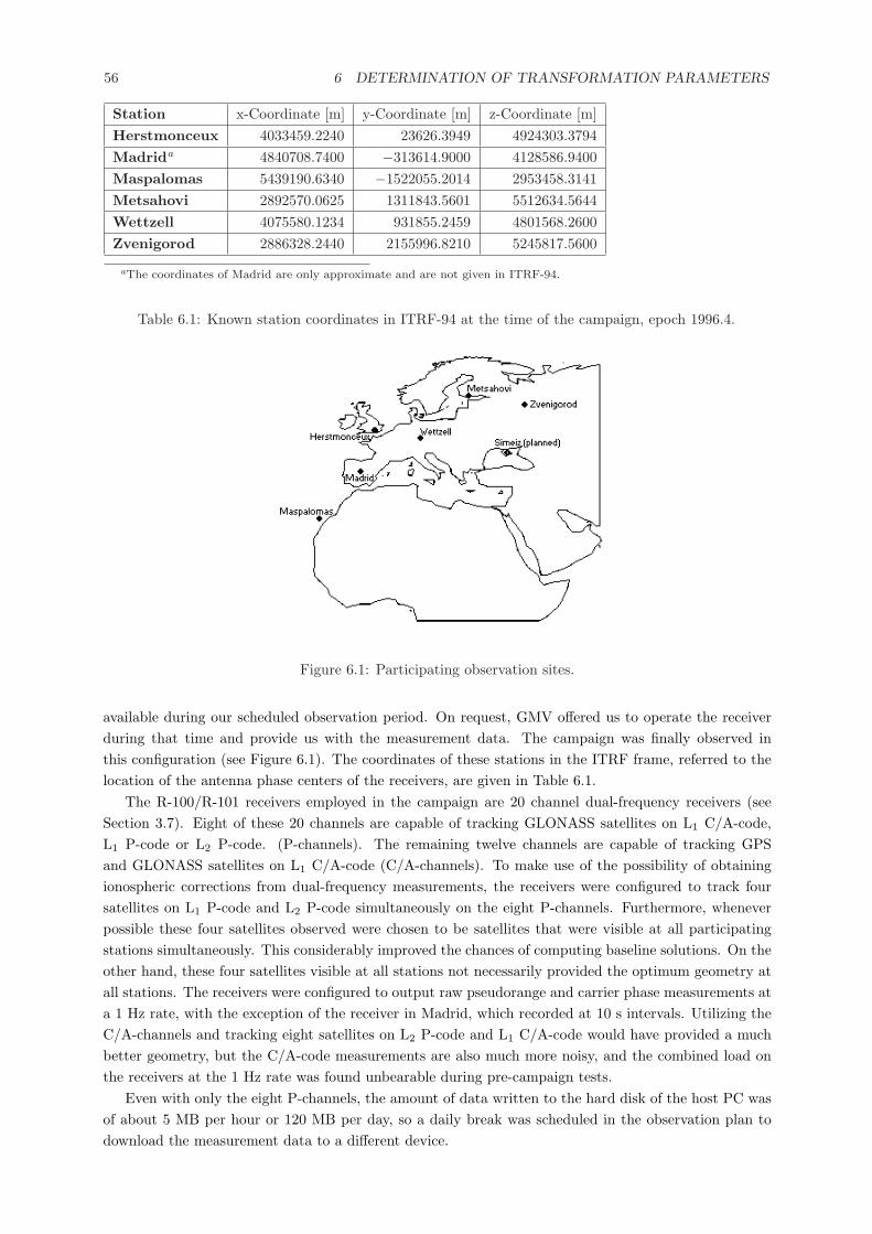
56 6 DETERMINATION OF TRANSFORMATION PARAMETERS
Station x-Coordinate [m] y-Coordinate [m] z-Coordinate [m]Herstmonceux 4033459.2240 23626.3949 4924303.3794Madrida 4840708.7400 −313614.9000 4128586.9400Maspalomas 5439190.6340 −1522055.2014 2953458.3141Metsahovi 2892570.0625 1311843.5601 5512634.5644Wettzell 4075580.1234 931855.2459 4801568.2600Zvenigorod 2886328.2440 2155996.8210 5245817.5600
aThe coordinates of Madrid are only approximate and are not given in ITRF-94.
Table 6.1: Known station coordinates in ITRF-94 at the time of the campaign, epoch 1996.4.
Figure 6.1: Participating observation sites.
available during our scheduled observation period. On request, GMV offered us to operate the receiverduring that time and provide us with the measurement data. The campaign was finally observed inthis configuration (see Figure 6.1). The coordinates of these stations in the ITRF frame, referred to thelocation of the antenna phase centers of the receivers, are given in Table 6.1.
The R-100/R-101 receivers employed in the campaign are 20 channel dual-frequency receivers (seeSection 3.7). Eight of these 20 channels are capable of tracking GLONASS satellites on L1 C/A-code,L1 P-code or L2 P-code. (P-channels). The remaining twelve channels are capable of tracking GPSand GLONASS satellites on L1 C/A-code (C/A-channels). To make use of the possibility of obtainingionospheric corrections from dual-frequency measurements, the receivers were configured to track foursatellites on L1 P-code and L2 P-code simultaneously on the eight P-channels. Furthermore, wheneverpossible these four satellites observed were chosen to be satellites that were visible at all participatingstations simultaneously. This considerably improved the chances of computing baseline solutions. On theother hand, these four satellites visible at all stations not necessarily provided the optimum geometry atall stations. The receivers were configured to output raw pseudorange and carrier phase measurements ata 1 Hz rate, with the exception of the receiver in Madrid, which recorded at 10 s intervals. Utilizing theC/A-channels and tracking eight satellites on L2 P-code and L1 C/A-code would have provided a muchbetter geometry, but the C/A-code measurements are also much more noisy, and the combined load onthe receivers at the 1 Hz rate was found unbearable during pre-campaign tests.
Even with only the eight P-channels, the amount of data written to the hard disk of the host PC wasof about 5 MB per hour or 120 MB per day, so a daily break was scheduled in the observation plan todownload the measurement data to a different device.
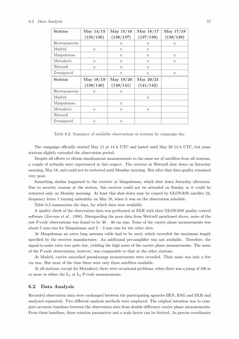
6.2 Data Analysis 57
Station May 14/15 May 15/16 May 16/17 May 17/18(135/136) (136/137) (137/138) (138/139)
Herstmonceux x x xMadrid x x xMaspalomas x x xMetsahovi x x x xWettzell x x xZvenigorod x x x
Station May 18/19 May 19/20 May 20/21(139/140) (140/141) (141/142)
Herstmonceux x xMadrid xMaspalomas xMetsahovi x x xWettzellZvenigorod x x
Table 6.2: Summary of available observations at stations by campaign day.
The campaign officially started May 15 at 14 h UTC and lasted until May 20 14 h UTC, but somestations slightly extended the observation period.
Despite all efforts to obtain simultaneous measurements to the same set of satellites from all stations,a couple of setbacks were experienced in this respect. The receiver at Wettzell shut down on Saturdaymorning, May 18, and could not be restarted until Monday morning. But after that data quality remainedvery poor.
Something similar happened to the receiver at Maspalomas, which shut down Saturday afternoon.Due to security reasons at the station, this receiver could not be attended on Sunday so it could berestarted only on Monday morning. At least this shut-down may be caused by GLONASS satellite 24,frequency letter 1 turning unhealthy on May 18, when it was on the observation schedule.
Table 6.2 summarizes the days, for which data were available.A quality check of the observation data was performed at DLR with their GLONASS quality control
software (Zarraoa et al., 1996). Disregarding the poor data from Wettzell mentioned above, noise of theraw P-code observations was found to be 30 – 40 cm rms. Noise of the carrier phase measurements wasabout 5 mm rms for Maspalomas and 2 – 3 mm rms for the other sites.
At Maspalomas an extra long antenna cable had to be used, which exceeded the maximum lengthspecified by the receiver manufacturer. An additional pre-amplifier was not available. Therefore, thesignal-to-noise ratio was quite low, yielding the high noise of the carrier phase measurements. The noiseof the P-code observations, however, was comparable to that at the other stations.
At Madrid, carrier smoothed pseudorange measurements were recorded. Their noise was only a fewcm rms. But most of the time there were only three satellites available.
At all stations, except for Metsahovi, there were occasional problems, when there was a jump of 100 mor more in either the L1 or L2 P-code measurements.
6.2 Data Analysis
Recorded observation data were exchanged between the participating agencies IfEN, IfAG and DLR andanalyzed separately. Two different analysis methods were employed. The original intention was to com-pute accurate baselines between the observation sites from double difference carrier phase measurements.From these baselines, three rotation parameters and a scale factor can be derived. As precise coordinates
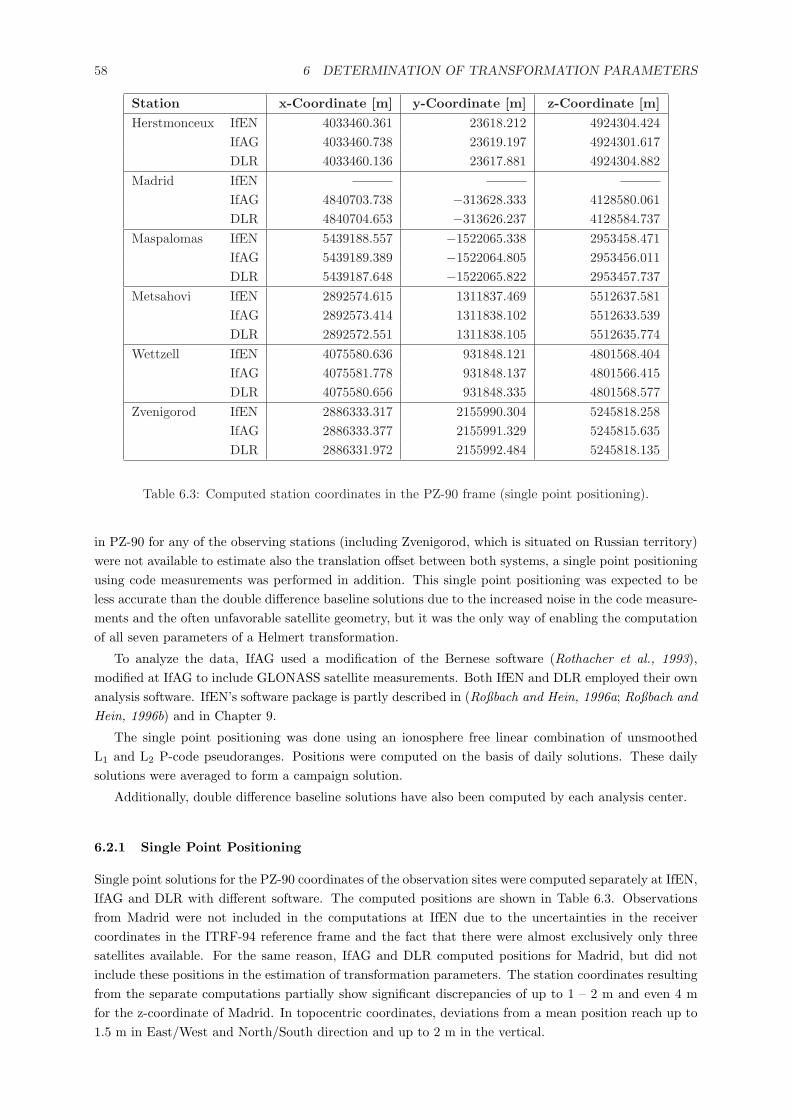
58 6 DETERMINATION OF TRANSFORMATION PARAMETERS
Station x-Coordinate [m] y-Coordinate [m] z-Coordinate [m]Herstmonceux IfEN 4033460.361 23618.212 4924304.424
IfAG 4033460.738 23619.197 4924301.617DLR 4033460.136 23617.881 4924304.882
Madrid IfENIfAG 4840703.738 −313628.333 4128580.061DLR 4840704.653 −313626.237 4128584.737
Maspalomas IfEN 5439188.557 −1522065.338 2953458.471IfAG 5439189.389 −1522064.805 2953456.011DLR 5439187.648 −1522065.822 2953457.737
Metsahovi IfEN 2892574.615 1311837.469 5512637.581IfAG 2892573.414 1311838.102 5512633.539DLR 2892572.551 1311838.105 5512635.774
Wettzell IfEN 4075580.636 931848.121 4801568.404IfAG 4075581.778 931848.137 4801566.415DLR 4075580.656 931848.335 4801568.577
Zvenigorod IfEN 2886333.317 2155990.304 5245818.258IfAG 2886333.377 2155991.329 5245815.635DLR 2886331.972 2155992.484 5245818.135
Table 6.3: Computed station coordinates in the PZ-90 frame (single point positioning).
in PZ-90 for any of the observing stations (including Zvenigorod, which is situated on Russian territory)were not available to estimate also the translation offset between both systems, a single point positioningusing code measurements was performed in addition. This single point positioning was expected to beless accurate than the double difference baseline solutions due to the increased noise in the code measure-ments and the often unfavorable satellite geometry, but it was the only way of enabling the computationof all seven parameters of a Helmert transformation.
To analyze the data, IfAG used a modification of the Bernese software (Rothacher et al., 1993),modified at IfAG to include GLONASS satellite measurements. Both IfEN and DLR employed their ownanalysis software. IfEN’s software package is partly described in (Roßbach and Hein, 1996a; Roßbach andHein, 1996b) and in Chapter 9.
The single point positioning was done using an ionosphere free linear combination of unsmoothedL1 and L2 P-code pseudoranges. Positions were computed on the basis of daily solutions. These dailysolutions were averaged to form a campaign solution.
Additionally, double difference baseline solutions have also been computed by each analysis center.
6.2.1 Single Point Positioning
Single point solutions for the PZ-90 coordinates of the observation sites were computed separately at IfEN,IfAG and DLR with different software. The computed positions are shown in Table 6.3. Observationsfrom Madrid were not included in the computations at IfEN due to the uncertainties in the receivercoordinates in the ITRF-94 reference frame and the fact that there were almost exclusively only threesatellites available. For the same reason, IfAG and DLR computed positions for Madrid, but did notinclude these positions in the estimation of transformation parameters. The station coordinates resultingfrom the separate computations partially show significant discrepancies of up to 1 – 2 m and even 4 mfor the z-coordinate of Madrid. In topocentric coordinates, deviations from a mean position reach up to1.5 m in East/West and North/South direction and up to 2 m in the vertical.
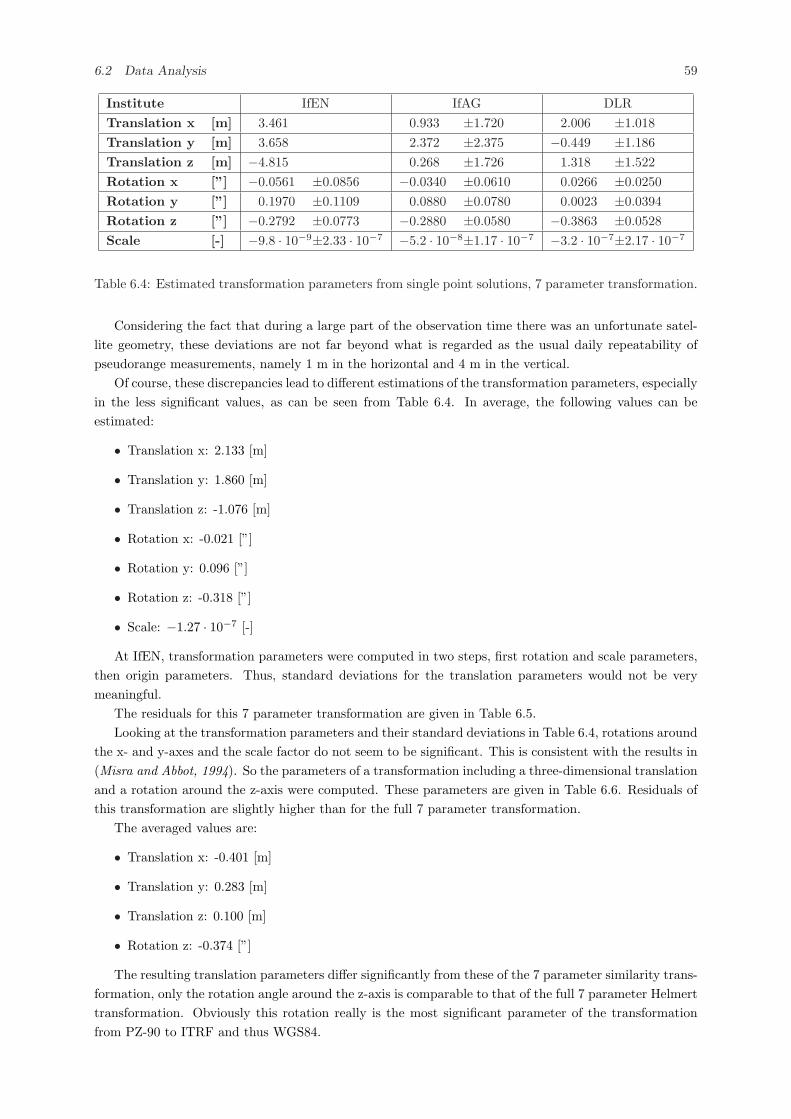
6.2 Data Analysis 59
Institute IfEN IfAG DLRTranslation x [m] 3.461 0.933 ±1.720 2.006 ±1.018Translation y [m] 3.658 2.372 ±2.375 −0.449 ±1.186Translation z [m] −4.815 0.268 ±1.726 1.318 ±1.522Rotation x [”] −0.0561 ±0.0856 −0.0340 ±0.0610 0.0266 ±0.0250Rotation y [”] 0.1970 ±0.1109 0.0880 ±0.0780 0.0023 ±0.0394Rotation z [”] −0.2792 ±0.0773 −0.2880 ±0.0580 −0.3863 ±0.0528Scale [-] −9.8 · 10−9±2.33 · 10−7 −5.2 · 10−8±1.17 · 10−7 −3.2 · 10−7±2.17 · 10−7
Table 6.4: Estimated transformation parameters from single point solutions, 7 parameter transformation.
Considering the fact that during a large part of the observation time there was an unfortunate satel-lite geometry, these deviations are not far beyond what is regarded as the usual daily repeatability ofpseudorange measurements, namely 1 m in the horizontal and 4 m in the vertical.
Of course, these discrepancies lead to different estimations of the transformation parameters, especiallyin the less significant values, as can be seen from Table 6.4. In average, the following values can beestimated:
• Translation x: 2.133 [m]
• Translation y: 1.860 [m]
• Translation z: -1.076 [m]
• Rotation x: -0.021 [”]
• Rotation y: 0.096 [”]
• Rotation z: -0.318 [”]
• Scale: −1.27 · 10−7 [-]
At IfEN, transformation parameters were computed in two steps, first rotation and scale parameters,then origin parameters. Thus, standard deviations for the translation parameters would not be verymeaningful.
The residuals for this 7 parameter transformation are given in Table 6.5.Looking at the transformation parameters and their standard deviations in Table 6.4, rotations around
the x- and y-axes and the scale factor do not seem to be significant. This is consistent with the results in(Misra and Abbot, 1994). So the parameters of a transformation including a three-dimensional translationand a rotation around the z-axis were computed. These parameters are given in Table 6.6. Residuals ofthis transformation are slightly higher than for the full 7 parameter transformation.
The averaged values are:
• Translation x: -0.401 [m]
• Translation y: 0.283 [m]
• Translation z: 0.100 [m]
• Rotation z: -0.374 [”]
The resulting translation parameters differ significantly from these of the 7 parameter similarity trans-formation, only the rotation angle around the z-axis is comparable to that of the full 7 parameter Helmerttransformation. Obviously this rotation really is the most significant parameter of the transformationfrom PZ-90 to ITRF and thus WGS84.
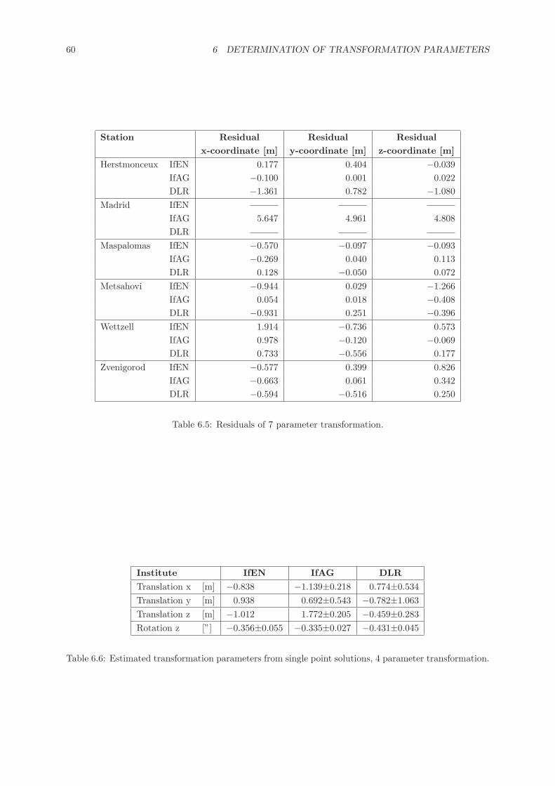
60 6 DETERMINATION OF TRANSFORMATION PARAMETERS
Station Residual Residual Residualx-coordinate [m] y-coordinate [m] z-coordinate [m]
Herstmonceux IfEN 0.177 0.404 −0.039IfAG −0.100 0.001 0.022DLR −1.361 0.782 −1.080
Madrid IfENIfAG 5.647 4.961 4.808DLR
Maspalomas IfEN −0.570 −0.097 −0.093IfAG −0.269 0.040 0.113DLR 0.128 −0.050 0.072
Metsahovi IfEN −0.944 0.029 −1.266IfAG 0.054 0.018 −0.408DLR −0.931 0.251 −0.396
Wettzell IfEN 1.914 −0.736 0.573IfAG 0.978 −0.120 −0.069DLR 0.733 −0.556 0.177
Zvenigorod IfEN −0.577 0.399 0.826IfAG −0.663 0.061 0.342DLR −0.594 −0.516 0.250
Table 6.5: Residuals of 7 parameter transformation.
Institute IfEN IfAG DLRTranslation x [m] −0.838 −1.139±0.218 0.774±0.534Translation y [m] 0.938 0.692±0.543 −0.782±1.063Translation z [m] −1.012 1.772±0.205 −0.459±0.283Rotation z [”] −0.356±0.055 −0.335±0.027 −0.431±0.045
Table 6.6: Estimated transformation parameters from single point solutions, 4 parameter transformation.
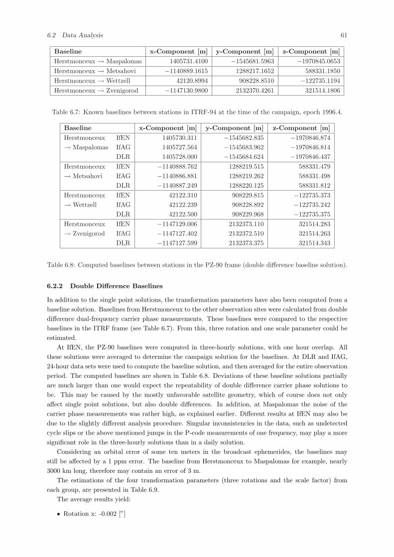
6.2 Data Analysis 61
Baseline x-Component [m] y-Component [m] z-Component [m]Herstmonceux → Maspalomas 1405731.4100 −1545681.5963 −1970845.0653Herstmonceux → Metsahovi −1140889.1615 1288217.1652 588331.1850Herstmonceux → Wettzell 42120.8994 908228.8510 −122735.1194Herstmonceux → Zvenigorod −1147130.9800 2132370.4261 321514.1806
Table 6.7: Known baselines between stations in ITRF-94 at the time of the campaign, epoch 1996.4.
Baseline x-Component [m] y-Component [m] z-Component [m]Herstmonceux IfEN 1405730.311 −1545682.835 −1970846.874→ Maspalomas IfAG 1405727.564 −1545683.962 −1970846.814
DLR 1405728.000 −1545684.624 −1970846.437Herstmonceux IfEN −1140888.762 1288219.515 588331.479→ Metsahovi IfAG −1140886.881 1288219.262 588331.498
DLR −1140887.249 1288220.125 588331.812Herstmonceux IfEN 42122.310 908229.815 −122735.373→ Wettzell IfAG 42122.239 908228.892 −122735.242
DLR 42122.500 908229.968 −122735.375Herstmonceux IfEN −1147129.006 2132373.110 321514.283→ Zvenigorod IfAG −1147127.402 2132372.510 321514.263
DLR −1147127.599 2132373.375 321514.343
Table 6.8: Computed baselines between stations in the PZ-90 frame (double difference baseline solution).
6.2.2 Double Difference Baselines
In addition to the single point solutions, the transformation parameters have also been computed from abaseline solution. Baselines from Herstmonceux to the other observation sites were calculated from doubledifference dual-frequency carrier phase measurements. These baselines were compared to the respectivebaselines in the ITRF frame (see Table 6.7). From this, three rotation and one scale parameter could beestimated.
At IfEN, the PZ-90 baselines were computed in three-hourly solutions, with one hour overlap. Allthese solutions were averaged to determine the campaign solution for the baselines. At DLR and IfAG,24-hour data sets were used to compute the baseline solution, and then averaged for the entire observationperiod. The computed baselines are shown in Table 6.8. Deviations of these baseline solutions partiallyare much larger than one would expect the repeatability of double difference carrier phase solutions tobe. This may be caused by the mostly unfavorable satellite geometry, which of course does not onlyaffect single point solutions, but also double differences. In addition, at Maspalomas the noise of thecarrier phase measurements was rather high, as explained earlier. Different results at IfEN may also bedue to the slightly different analysis procedure. Singular inconsistencies in the data, such as undetectedcycle slips or the above mentioned jumps in the P-code measurements of one frequency, may play a moresignificant role in the three-hourly solutions than in a daily solution.
Considering an orbital error of some ten meters in the broadcast ephemerides, the baselines maystill be affected by a 1 ppm error. The baseline from Herstmonceux to Maspalomas for example, nearly3000 km long, therefore may contain an error of 3 m.
The estimations of the four transformation parameters (three rotations and the scale factor) fromeach group, are presented in Table 6.9.
The average results yield:
• Rotation x: -0.002 [”]
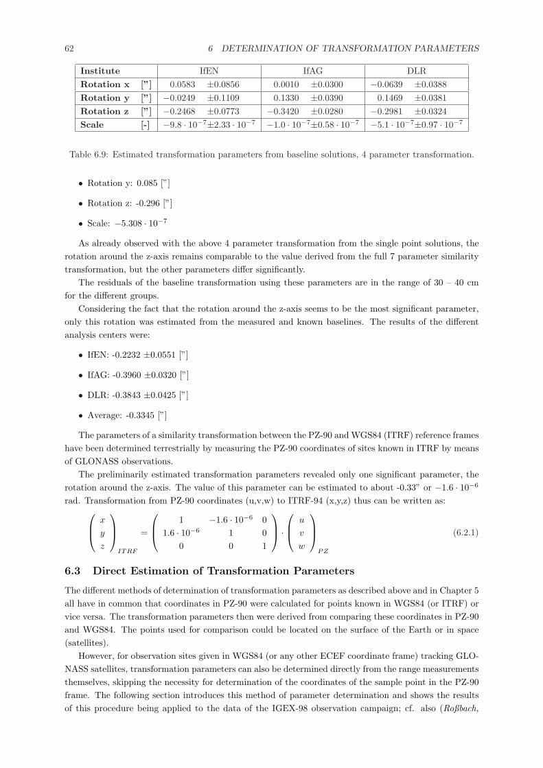
62 6 DETERMINATION OF TRANSFORMATION PARAMETERS
Institute IfEN IfAG DLRRotation x [”] 0.0583 ±0.0856 0.0010 ±0.0300 −0.0639 ±0.0388Rotation y [”] −0.0249 ±0.1109 0.1330 ±0.0390 0.1469 ±0.0381Rotation z [”] −0.2468 ±0.0773 −0.3420 ±0.0280 −0.2981 ±0.0324Scale [-] −9.8 · 10−7±2.33 · 10−7 −1.0 · 10−7±0.58 · 10−7 −5.1 · 10−7±0.97 · 10−7
Table 6.9: Estimated transformation parameters from baseline solutions, 4 parameter transformation.
• Rotation y: 0.085 [”]
• Rotation z: -0.296 [”]
• Scale: −5.308 · 10−7
As already observed with the above 4 parameter transformation from the single point solutions, therotation around the z-axis remains comparable to the value derived from the full 7 parameter similaritytransformation, but the other parameters differ significantly.
The residuals of the baseline transformation using these parameters are in the range of 30 – 40 cmfor the different groups.
Considering the fact that the rotation around the z-axis seems to be the most significant parameter,only this rotation was estimated from the measured and known baselines. The results of the differentanalysis centers were:
• IfEN: -0.2232 ±0.0551 [”]
• IfAG: -0.3960 ±0.0320 [”]
• DLR: -0.3843 ±0.0425 [”]
• Average: -0.3345 [”]
The parameters of a similarity transformation between the PZ-90 and WGS84 (ITRF) reference frameshave been determined terrestrially by measuring the PZ-90 coordinates of sites known in ITRF by meansof GLONASS observations.
The preliminarily estimated transformation parameters revealed only one significant parameter, therotation around the z-axis. The value of this parameter can be estimated to about -0.33” or −1.6 · 10−6
rad. Transformation from PZ-90 coordinates (u,v,w) to ITRF-94 (x,y,z) thus can be written as:
x
y
z
ITRF
=
1 −1.6 · 10−6 01.6 · 10−6 1 0
0 0 1
·
u
v
w
PZ
(6.2.1)
6.3 Direct Estimation of Transformation Parameters
The different methods of determination of transformation parameters as described above and in Chapter 5all have in common that coordinates in PZ-90 were calculated for points known in WGS84 (or ITRF) orvice versa. The transformation parameters then were derived from comparing these coordinates in PZ-90and WGS84. The points used for comparison could be located on the surface of the Earth or in space(satellites).
However, for observation sites given in WGS84 (or any other ECEF coordinate frame) tracking GLO-NASS satellites, transformation parameters can also be determined directly from the range measurementsthemselves, skipping the necessity for determination of the coordinates of the sample point in the PZ-90frame. The following section introduces this method of parameter determination and shows the resultsof this procedure being applied to the data of the IGEX-98 observation campaign; cf. also (Roßbach,
6.3 Direct Estimation of Transformation Parameters 63
1999). Originally, a set of transformation parameters was to be derived from data of the measurementcampaign described above using this method. However, the much better geometry of the IGEX sitesprovided significantly better results.
The principle of direct determination of the transformation parameters is shown for station coordinatesgiven in WGS84. It can, however, be applied to any other ECEF coordinate frame as well. In the IGEX-98 campaign, coordinates of the observation sites were given in ITRF-96. Thus, the results of this processwill be a set of transformation parameters from PZ-90 to ITRF-96. However, ITRF-96 and WGS84 canbe regarded as identical.
The (simplified) pseudorange observation equation from receiver R to satellite S is given by
PRSR = %S
R + c · δtR − c · δtS + c · δtS,TropR + c · δtS,Iono
R (6.3.1)
with
%SR =
√(xR − xS)2 + (yR − yS)2 + (zR − zS)2 (6.3.2)
The position vectors of receiver ~xR and satellite ~xS in Eq. (6.3.2) must be given in the same coordinateframe.
In the given case of direct determination of transformation parameters between PZ-90 and WGS84from range measurements to GLONASS satellites, the known coordinates of the observation sites aregiven in WGS84, whereas the coordinates of the GLONASS satellites are determined from ephemerisdata and are given in PZ-90. Since both WGS84 and PZ-90 are Earth-centered Earth-fixed (ECEF)coordinate frames, they rotate along with the Earth. Their orientation therefore is a function of time.More precise, thus, the coordinates of the observation sites are given in WGS84, as valid at the timeof signal reception tRX , and the coordinates of the satellites are given in PZ-90, as valid at the time ofsignal transmission tTX .
~xR = ~xR,WGS(tRX)
~xS = ~xSPZ(tT X)
To obtain the actual geometrical distance from receiver to satellite, one of these two sets of coordinatesmust be transformed to the coordinate frame of the other set. Here it is chosen to transform the satellitecoordinates to the coordinate frame of the observer. This requires two steps of transformation:
• Transformation from PZ-90 to WGS84: ~xSPZ(tT X) → ~xS
WGS(tT X)
• Correction of Earth rotation: ~xSWGS(tT X) → ~xS
WGS(tRX)
Correction of Earth rotation
While the satellite signal is travelling towards the observer, the Earth – and along with it the Earth-fixed coordinate frame – keeps rotating. During this signal travel time, it rotates by an angle of α =%S
R/c · ωE . This is a positive rotation around the z-axis. Thus, the satellite coordinates transform by
~xSPZ(tRX) =
1 α 0−α 1 0
0 0 1
· ~xS
PZ(tT X) (6.3.3)
for small angles α.
The geometrical distance therefore becomes
%SR =
√(xR,PZ(tRX)−xS
PZ(tRX)
)2
+(yR,PZ(tRX)−yS
PZ(tRX)
)2
+(zR,PZ(tRX)−zS
PZ(tRX)
)2
(6.3.4)
64 6 DETERMINATION OF TRANSFORMATION PARAMETERS
or
%SR
2=
(xR,PZ(tRX)−xS
PZ(tT X)−ωE
c%S
R · ySPZ(tT X)
)2
+ (6.3.5)(yR,PZ(tRX)−yS
PZ(tT X)+ωE
c%S
R · xSPZ(tT X)
)2
+(zR,PZ(tRX)−zS
PZ(tT X)
)2
=(xR,PZ(tRX)−xS
PZ(tT X)
)2
−2(xR,PZ(tRX)−xS
PZ(tT X)
) ωE
c%S
RySPZ(tT X)+
ω2E
c2%S
R
2yS
PZ(tT X)
2+
(yR,PZ(tRX)−yS
PZ(tT X)
)2
+2(yR,PZ(tRX)−yS
PZ(tT X)
) ωE
c%S
RxSPZ(tT X)+
ω2E
c2%S
R
2xS
PZ(tT X)
2+
(zR,PZ(tRX)−zS
PZ(tT X)
)2
(6.3.6)
=(xR,PZ(tRX)−xS
PZ(tT X)
)2
+(yR,PZ(tRX)−yS
PZ(tT X)
)2
+(zR,PZ(tRX)−zS
PZ(tT X)
)2
+ (6.3.7)
ω2E
c2%S
R
2 ·(xS
PZ(tT X)
2+yS
PZ(tT X)
2)−2
ωE
c%S
R ·(xR,PZ(tRX)y
SPZ(tT X)−yR,PZ(tRX)x
SPZ(tT X)
)
This transforms into
0 = %SR
2 ·[1−
(ωE
c
)2 (xS
PZ(tT X)
2+ yS
PZ(tT X)
2)]
+
2ωE
c%S
R ·(xR,PZ(tRX)y
SPZ(tT X) − yR,PZ(tRX)x
SPZ(tT X)
)− (6.3.8)
(xR,PZ(tRX) − xS
PZ(tT X)
)2
−(yR,PZ(tRX) − yS
PZ(tT X)
)2
−(zR,PZ(tRX) − zS
PZ(tT X)
)2
The term(
ωE
c
)2 ·(xS
PZ(tT X)
2 + ySPZ(tT X)
2)
in Eq. (6.3.8) is of the order of magnitude 10−12 and canbe neglected with respect to the 1:
0 = %SR
2+ 2
ωE
c%S
R ·(xR,PZ(tRX)y
SPZ(tT X) − yR,PZ(tRX)x
SPZ(tT X)
)− (6.3.9)
(xR,PZ(tRX) − xS
PZ(tT X)
)2
−(yR,PZ(tRX) − yS
PZ(tT X)
)2
−(zR,PZ(tRX) − zS
PZ(tT X)
)2
This quadratic equation has two possible solutions:
%SR1,2 = −ωE
c·(xR,PZ(tRX)y
SPZ(tT X) − yR,PZ(tRX)x
SPZ(tT X)
)±
[(ωE
c
)2
·(xR,PZ(tRX)y
SPZ(tT X)−yR,PZ(tRX)x
SPZ(tT X)
)2
+ (6.3.10)
(xR,PZ(tRX)−xS
PZ(tT X)
)2
+(yR,PZ(tRX)−yS
PZ(tT X)
)2
+(zR,PZ(tRX)−zS
PZ(tT X)
)2]1/2
Since the square root is always positive and of larger magnitude than the term in front of it, thenegative sign in front of the square root does not provide a physically meaningful solution. Therefore thedistance between satellite and observer, corrected for Earth rotation during the signal travel time, canbe written as:
%SR = −ωE
c·(xR,PZ(tRX)y
SPZ(tT X)−yR,PZ(tRX)x
SPZ(tT X)
)+
[(ωE
c
)2
·(xR,PZ(tRX)y
SPZ(tT X)−yR,PZ(tRX)x
SPZ(tT X)
)2
+ (6.3.11)
(xR,PZ(tRX)−xS
PZ(tT X)
)2
+(yR,PZ(tRX)−yS
PZ(tT X)
)2
+(zR,PZ(tRX)−zS
PZ(tT X)
)2]1/2
For deriving Eq. (6.3.11), the PZ-90 coordinate frame was used. Of course, Eq. (6.3.11) is also valid inthe WGS84 coordinate frame:
%SR = −ωE
c·(xR,WGS(tRX)y
SWGS(tT X)−yR,WGS(tRX)x
SWGS(tT X)
)+
[(ωE
c
)2·(xR,WGS(tRX)y
SWGS(tT X)−yR,WGS(tRX)x
SWGS(tT X)
)2
+ (6.3.12)
(xR,WGS(tRX)−xS
WGS(tT X)
)2+
(yR,WGS(tRX)−yS
WGS(tT X)
)2+
(zR,WGS(tRX)−zS
WGS(tT X)
)2]1/2
6.3 Direct Estimation of Transformation Parameters 65
Transformation from PZ-90 to WGS84The transformation of a position vector given in PZ-90 to WGS84 can be written as (cf. Section 5.5):
x
y
z
WGS
=
∆x
∆y
∆z
+ (1 + δs) ·
1 δω −δψ
−δω 1 δε
δψ −δε 1
·
x
y
z
PZ
(6.3.13)
or in individual coordinates, valid at time tTX :
xSWGS(tT X) = ∆x + (1 + δs) ·
(xS
PZ(tT X) + δω · ySPZ(tT X) − δψ · zS
PZ(tT X)
)
ySWGS(tT X) = ∆y + (1 + δs) ·
(−δω · xS
PZ(tT X) + ySPZ(tT X) + δε · zS
PZ(tT X)
)(6.3.14)
zSWGS(tT X) = ∆z + (1 + δs) ·
(δψ · xS
PZ(tT X) − δε · ySPZ(tT X) + zS
PZ(tT X)
)
Inserting this into Eq. (6.3.12) yields
%SR = −ωE
c
{xR,WGS(tRX)
[∆y + (1+δs) ·
(−δω · xS
PZ(tT X) + ySPZ(tT X) + δε · zS
PZ(tT X)
)]−
yR,WGS(tRX)
[∆x + (1+δs) ·
(xS
PZ(tT X) + δω · ySPZ(tT X) − δψ · zS
PZ(tT X)
)]}+
[(ωE
c
)2 {xR,WGS(tRX)
[∆y + (1+δs) ·
(−δω · xS
PZ(tT X) + ySPZ(tT X) + δε · zS
PZ(tT X)
)]−
yR,WGS(tRX)
[∆x + (1+δs) ·
(xS
PZ(tT X) + δω · ySPZ(tT X) − δψ · zS
PZ(tT X)
)]}2
+ (6.3.15){
xR,WGS(tRX) −[∆x + (1+δs) ·
(xS
PZ(tT X) + δω · ySPZ(tT X) − δψ · zS
PZ(tT X)
)]}2
+{
yR,WGS(tRX) −[∆y + (1+δs) ·
(−δω · xS
PZ(tT X) + ySPZ(tT X) + δε · zS
PZ(tT X)
)]}2
+
{zR,WGS(tRX) −
[∆z + (1+δs) ·
(δψ · xS
PZ(tT X) − δε · ySPZ(tT X) + zS
PZ(tT X)
)]}2]1/2
Here, the coordinates ~xR,WGS(tRX) are the known station coordinates, given in WGS84, valid atthe time of signal reception. ~xS
PZ(tT X) are the satellite coordinates at the time of signal transmission asobtained from ephemeris data. They are given in the PZ-90 frame, valid at the time of signal transmission.The transformation parameters ∆x, ∆y, ∆z, δs, δε, δψ, δω are unknown in this geometrical range indifferent coordinate frames Eq. (6.3.15). Inserting this geometrical range into the observation equationEq. (6.3.1), these unknowns can be solved for, provided there is a sufficient number of observations.However, the receiver clock error δtR in Eq. (6.3.1) is also unknown. The satellite clock error δtS
can be determined from ephemeris data, whereas tropospheric and ionospheric path delays δtS,TropR and
δtS,IonoR can be modelled. Since GLONASS offers free and unobstructed access to the second frequency,
dual-frequency ionospheric corrections can be applied alternatively.This leaves seven unknown transformation parameters and one unknown receiver clock error to solve
for. Thus, with range measurements to eight GLONASS satellites at one observation site, a completeset of transformation parameters could be determined. Besides having eight GLONASS satellites in viewis rather unlikely in times of depleted GLONASS constellation, this one observation site will provide apoor geometry to separate origin and orientation parameters. As discussed in Section 5.6.1, this will leadto a set of parameters that are only valid at a small area around the observation site. More stationswill add more strength to the geometry. However, each additional observation site does also mean anadditional receiver and thus one more receiver clock error as a further unknown. For simultaneousobservations at five stations, as was the case during the IfEN/IfAG/DLR measurement campaign, thistotals in twelve unknowns. Thus, with two to three observations at each station, it was possible todetermine the transformation parameters directly from pseudorange observations. With seven or moreobservation sites, which can easily be reached with data from the IGEX campaign, only two satellitesin view per site are required. This is another bonus of this method for determining the transformation
66 6 DETERMINATION OF TRANSFORMATION PARAMETERS
parameters: For the conventional method of determining point coordinates in PZ-90 from GLONASSsatellite observations and then comparing these coordinates to known coordinates in WGS84, requires atleast four satellites visible at a station to calculate station coordinates. This approach of direct estimationof the transformation parameters may work with as little as two observations per site. Depending on thenumber of stations involved, at some sites only one observation may mathematically be sufficient to geta solution, but this one measurement contributes only to the station clock error.
The geometrical range Eq. (6.3.15) and with it the observation equation Eq. (6.3.1) is non-linear inthe unknown transformation parameters. Before trying to solve a system of observation equations, theEq. (6.3.15) has to be linearized. Therefore, this equation is expanded in a Taylor series around theapproximate values ∆x0, ∆y0, ∆z0, δs0, δε0, δψ0, δω0:
%SR(∆x, ∆y, ∆z, δs, δε, δψ, δω) = %S
R,0 +∂%S
R
∂∆x
∣∣∣∣0
· (∆x−∆x0) +∂%S
R
∂∆y
∣∣∣∣0
· (∆y −∆y0)+
∂%SR
∂∆z
∣∣∣∣0
· (∆z −∆z0) +∂%S
R
∂δs
∣∣∣∣0
· (δs− δs0) +∂%S
R
∂δε
∣∣∣∣0
· (δε− δε0) + (6.3.16)
∂%SR
∂δψ
∣∣∣∣0
· (δψ − δψ0) +∂%S
R
∂δω
∣∣∣∣0
· (δω − δω0)
with
%SR,0 = %S
R(∆x0,∆y0,∆z0, δs0, δε0, δψ0, δω0)
∂%SR
∂d
∣∣∣∣0
=∂%S
R
∂d(∆x0, ∆y0,∆z0, δs0, δε0, δψ0, δω0), d ∈ {∆x, ∆y, ∆z, δs, δε, δψ, δω}
For reasons of simplicity, Eq. (6.3.15) is not differentiated directly. Rather it is preferred to differen-tiate Eq. (6.3.14) and then insert the results into the differentiated Eq. (6.3.12).
Differentiating Eq. (6.3.12) by any of the unknown transformation parameters d, d ∈ {∆x, ∆y, ∆z,
δs, δε, δψ, δω} yields:
∂%SR
∂d
∣∣∣∣0
= −ωE
c·(
xR,WGS(tRX) ·∂yS
WGS(tT X)
∂d
∣∣∣∣∣0
− yR,WGS(tRX) ·∂xS
WGS(tT X)
∂d
∣∣∣∣∣0
)+
1S0
·[(ωE
c
)2
s0 ·(
xR,WGS(tRX) ·∂yS
WGS(tT X)
∂d
∣∣∣∣∣0
− yR,WGS(tRX) ·∂xS
WGS(tT X)
∂d
∣∣∣∣∣0
)− (6.3.17)
ξ0 ·∂xS
WGS(tT X)
∂d
∣∣∣∣∣0
− υ0 ·∂yS
WGS(tT X)
∂d
∣∣∣∣∣0
− ζ0 ·∂zS
WGS(tT X)
∂d
∣∣∣∣∣0
]
with
S0 =
√(ωE
c
)2
· s20 + ξ2
0 + υ20 + ζ2
0
s0 = xR,WGS(tRX) · ySWGS(tT X),0 − yR,WGS(tRX) · xS
WGS(tT X),0
= xR,WGS(tRX) ·[∆y0 + (1 + δs0) ·
(−δω0 · xS
PZ(tT X) + ySPZ(tT X) + δε0 · zS
PZ(tT X)
)]−
yR,WGS(tRX) ·[∆x0 + (1 + δs0) ·
(xS
PZ(tT X) + δω0 · ySPZ(tT X) − δψ0 · zS
PZ(tT X)
)]
ξ0 = xR,WGS(tRX) − xSWGS(tT X),0
= xR,WGS(tRX) −∆x0 − (1 + δs0) ·(xS
PZ(tT X) + δω0 · ySPZ(tT X) − δψ0 · zS
PZ(tT X)
)
υ0 = yR,WGS(tRX) − ySWGS(tT X),0
= yR,WGS(tRX) −∆y0 − (1 + δs0) ·(−δω0 · xS
PZ(tT X) + ySPZ(tT X) + δε0 · zS
PZ(tT X)
)
ζ0 = zR,WGS(tRX) − zSWGS(tT X),0
= zR,WGS(tRX) −∆z0 − (1 + δs0) ·(δψ0 · xS
PZ(tT X) − δε0 · ySPZ(tT X) + zS
PZ(tT X)
)
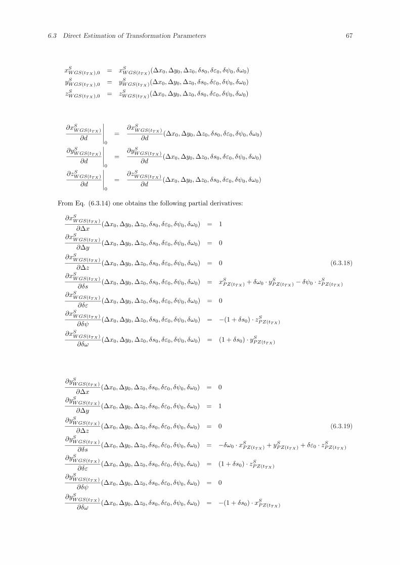
6.3 Direct Estimation of Transformation Parameters 67
xSWGS(tT X),0 = xS
WGS(tT X)(∆x0, ∆y0, ∆z0, δs0, δε0, δψ0, δω0)
ySWGS(tT X),0 = yS
WGS(tT X)(∆x0,∆y0, ∆z0, δs0, δε0, δψ0, δω0)
zSWGS(tT X),0 = zS
WGS(tT X)(∆x0, ∆y0, ∆z0, δs0, δε0, δψ0, δω0)
∂xSWGS(tT X)
∂d
∣∣∣∣∣0
=∂xS
WGS(tT X)
∂d(∆x0, ∆y0, ∆z0, δs0, δε0, δψ0, δω0)
∂ySWGS(tT X)
∂d
∣∣∣∣∣0
=∂yS
WGS(tT X)
∂d(∆x0,∆y0, ∆z0, δs0, δε0, δψ0, δω0)
∂zSWGS(tT X)
∂d
∣∣∣∣∣0
=∂zS
WGS(tT X)
∂d(∆x0, ∆y0, ∆z0, δs0, δε0, δψ0, δω0)
From Eq. (6.3.14) one obtains the following partial derivatives:
∂xSWGS(tT X)
∂∆x(∆x0, ∆y0, ∆z0, δs0, δε0, δψ0, δω0) = 1
∂xSWGS(tT X)
∂∆y(∆x0, ∆y0, ∆z0, δs0, δε0, δψ0, δω0) = 0
∂xSWGS(tT X)
∂∆z(∆x0, ∆y0, ∆z0, δs0, δε0, δψ0, δω0) = 0 (6.3.18)
∂xSWGS(tT X)
∂δs(∆x0, ∆y0, ∆z0, δs0, δε0, δψ0, δω0) = xS
PZ(tT X) + δω0 · ySPZ(tT X) − δψ0 · zS
PZ(tT X)
∂xSWGS(tT X)
∂δε(∆x0, ∆y0, ∆z0, δs0, δε0, δψ0, δω0) = 0
∂xSWGS(tT X)
∂δψ(∆x0, ∆y0, ∆z0, δs0, δε0, δψ0, δω0) = −(1 + δs0) · zS
PZ(tT X)
∂xSWGS(tT X)
∂δω(∆x0, ∆y0, ∆z0, δs0, δε0, δψ0, δω0) = (1 + δs0) · yS
PZ(tT X)
∂ySWGS(tT X)
∂∆x(∆x0, ∆y0, ∆z0, δs0, δε0, δψ0, δω0) = 0
∂ySWGS(tT X)
∂∆y(∆x0, ∆y0, ∆z0, δs0, δε0, δψ0, δω0) = 1
∂ySWGS(tT X)
∂∆z(∆x0, ∆y0, ∆z0, δs0, δε0, δψ0, δω0) = 0 (6.3.19)
∂ySWGS(tT X)
∂δs(∆x0, ∆y0, ∆z0, δs0, δε0, δψ0, δω0) = −δω0 · xS
PZ(tT X) + ySPZ(tT X) + δε0 · zS
PZ(tT X)
∂ySWGS(tT X)
∂δε(∆x0, ∆y0, ∆z0, δs0, δε0, δψ0, δω0) = (1 + δs0) · zS
PZ(tT X)
∂ySWGS(tT X)
∂δψ(∆x0, ∆y0, ∆z0, δs0, δε0, δψ0, δω0) = 0
∂ySWGS(tT X)
∂δω(∆x0, ∆y0, ∆z0, δs0, δε0, δψ0, δω0) = −(1 + δs0) · xS
PZ(tT X)
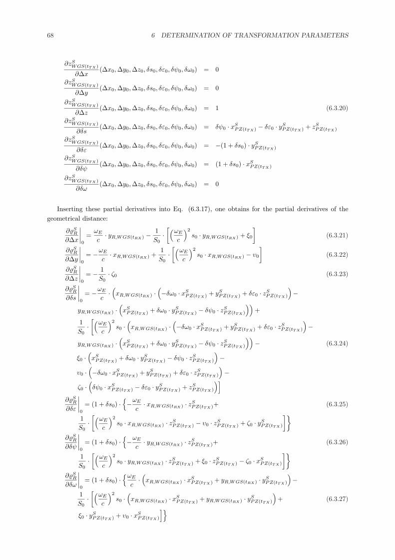
68 6 DETERMINATION OF TRANSFORMATION PARAMETERS
∂zSWGS(tT X)
∂∆x(∆x0, ∆y0, ∆z0, δs0, δε0, δψ0, δω0) = 0
∂zSWGS(tT X)
∂∆y(∆x0, ∆y0, ∆z0, δs0, δε0, δψ0, δω0) = 0
∂zSWGS(tT X)
∂∆z(∆x0, ∆y0, ∆z0, δs0, δε0, δψ0, δω0) = 1 (6.3.20)
∂zSWGS(tT X)
∂δs(∆x0, ∆y0, ∆z0, δs0, δε0, δψ0, δω0) = δψ0 · xS
PZ(tT X) − δε0 · ySPZ(tT X) + zS
PZ(tT X)
∂zSWGS(tT X)
∂δε(∆x0, ∆y0, ∆z0, δs0, δε0, δψ0, δω0) = −(1 + δs0) · yS
PZ(tT X)
∂zSWGS(tT X)
∂δψ(∆x0, ∆y0, ∆z0, δs0, δε0, δψ0, δω0) = (1 + δs0) · xS
PZ(tT X)
∂zSWGS(tT X)
∂δω(∆x0, ∆y0, ∆z0, δs0, δε0, δψ0, δω0) = 0
Inserting these partial derivatives into Eq. (6.3.17), one obtains for the partial derivatives of thegeometrical distance:
∂%SR
∂∆x
∣∣∣∣0
=ωE
c· yR,WGS(tRX) −
1S0
·[(ωE
c
)2
s0 · yR,WGS(tRX) + ξ0
](6.3.21)
∂%SR
∂∆y
∣∣∣∣0
= −ωE
c· xR,WGS(tRX) +
1S0
·[(ωE
c
)2
s0 · xR,WGS(tRX) − υ0
](6.3.22)
∂%SR
∂∆z
∣∣∣∣0
= − 1S0
· ζ0 (6.3.23)
∂%SR
∂δs
∣∣∣∣0
= −ωE
c·(xR,WGS(tRX) ·
(−δω0 · xS
PZ(tT X) + ySPZ(tT X) + δε0 · zS
PZ(tT X)
)−
yR,WGS(tRX) ·(xS
PZ(tT X) + δω0 · ySPZ(tT X) − δψ0 · zS
PZ(tT X)
))+
1S0
·[(ωE
c
)2
s0 ·(xR,WGS(tRX) ·
(−δω0 · xS
PZ(tT X) + ySPZ(tT X) + δε0 · zS
PZ(tT X)
)−
yR,WGS(tRX) ·(xS
PZ(tT X) + δω0 · ySPZ(tT X) − δψ0 · zS
PZ(tT X)
))− (6.3.24)
ξ0 ·(xS
PZ(tT X) + δω0 · ySPZ(tT X) − δψ0 · zS
PZ(tT X)
)−
υ0 ·(−δω0 · xS
PZ(tT X) + ySPZ(tT X) + δε0 · zS
PZ(tT X)
)−
ζ0 ·(δψ0 · xS
PZ(tT X) − δε0 · ySPZ(tT X) + zS
PZ(tT X)
)]
∂%SR
∂δε
∣∣∣∣0
= (1 + δs0) ·{−ωE
c· xR,WGS(tRX) · zS
PZ(tT X)+ (6.3.25)
1S0
·[(ωE
c
)2
s0 · xR,WGS(tRX) · zSPZ(tT X) − υ0 · zS
PZ(tT X) + ζ0 · ySPZ(tT X)
]}
∂%SR
∂δψ
∣∣∣∣0
= (1 + δs0) ·{−ωE
c· yR,WGS(tRX) · zS
PZ(tT X)+ (6.3.26)
1S0
·[(ωE
c
)2
s0 · yR,WGS(tRX) · zSPZ(tT X) + ξ0 · zS
PZ(tT X) − ζ0 · xSPZ(tT X)
]}
∂%SR
∂δω
∣∣∣∣0
= (1 + δs0) ·{ωE
c·(xR,WGS(tRX) · xS
PZ(tT X) + yR,WGS(tRX) · ySPZ(tT X)
)−
1S0
·[(ωE
c
)2
s0 ·(xR,WGS(tRX) · xS
PZ(tT X) + yR,WGS(tRX) · ySPZ(tT X)
)+ (6.3.27)
ξ0 · ySPZ(tT X) + υ0 · xS
PZ(tT X)
]}
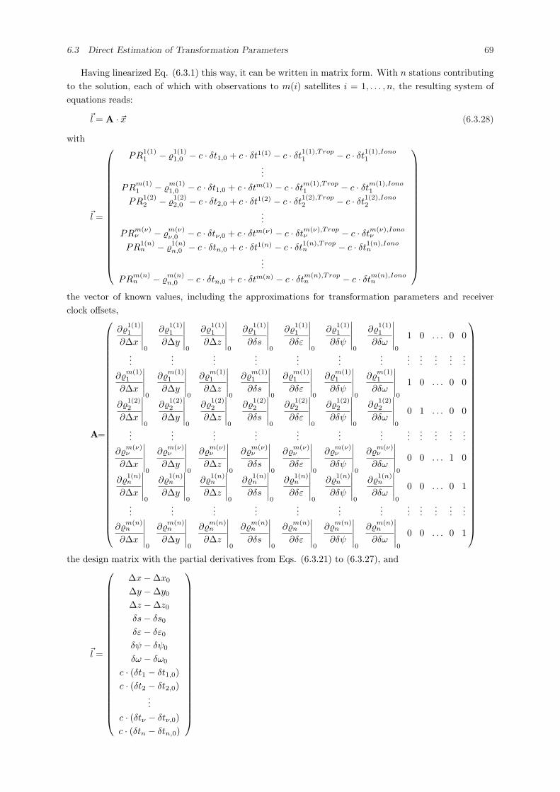
6.3 Direct Estimation of Transformation Parameters 69
Having linearized Eq. (6.3.1) this way, it can be written in matrix form. With n stations contributingto the solution, each of which with observations to m(i) satellites i = 1, . . . , n, the resulting system ofequations reads:
~l = A · ~x (6.3.28)
with
~l =
PR1(1)1 − %
1(1)1,0 − c · δt1,0 + c · δt1(1) − c · δt1(1),Trop
1 − c · δt1(1),Iono1
...PR
m(1)1 − %
m(1)1,0 − c · δt1,0 + c · δtm(1) − c · δtm(1),Trop
1 − c · δtm(1),Iono1
PR1(2)2 − %
1(2)2,0 − c · δt2,0 + c · δt1(2) − c · δt1(2),Trop
2 − c · δt1(2),Iono2
...PR
m(ν)ν − %
m(ν)ν,0 − c · δtν,0 + c · δtm(ν) − c · δtm(ν),Trop
ν − c · δtm(ν),Ionoν
PR1(n)n − %
1(n)n,0 − c · δtn,0 + c · δt1(n) − c · δt1(n),Trop
n − c · δt1(n),Ionon
...PR
m(n)n − %
m(n)n,0 − c · δtn,0 + c · δtm(n) − c · δtm(n),Trop
n − c · δtm(n),Ionon
the vector of known values, including the approximations for transformation parameters and receiverclock offsets,
A=
∂%1(1)1
∂∆x
∣∣∣∣∣0
∂%1(1)1
∂∆y
∣∣∣∣∣0
∂%1(1)1
∂∆z
∣∣∣∣∣0
∂%1(1)1
∂δs
∣∣∣∣∣0
∂%1(1)1
∂δε
∣∣∣∣∣0
∂%1(1)1
∂δψ
∣∣∣∣∣0
∂%1(1)1
∂δω
∣∣∣∣∣0
1 0 . . . 0 0
......
......
......
......
......
......
∂%m(1)1
∂∆x
∣∣∣∣∣0
∂%m(1)1
∂∆y
∣∣∣∣∣0
∂%m(1)1
∂∆z
∣∣∣∣∣0
∂%m(1)1
∂δs
∣∣∣∣∣0
∂%m(1)1
∂δε
∣∣∣∣∣0
∂%m(1)1
∂δψ
∣∣∣∣∣0
∂%m(1)1
∂δω
∣∣∣∣∣0
1 0 . . . 0 0
∂%1(2)2
∂∆x
∣∣∣∣∣0
∂%1(2)2
∂∆y
∣∣∣∣∣0
∂%1(2)2
∂∆z
∣∣∣∣∣0
∂%1(2)2
∂δs
∣∣∣∣∣0
∂%1(2)2
∂δε
∣∣∣∣∣0
∂%1(2)2
∂δψ
∣∣∣∣∣0
∂%1(2)2
∂δω
∣∣∣∣∣0
0 1 . . . 0 0
......
......
......
......
......
......
∂%m(ν)ν
∂∆x
∣∣∣∣∣0
∂%m(ν)ν
∂∆y
∣∣∣∣∣0
∂%m(ν)ν
∂∆z
∣∣∣∣∣0
∂%m(ν)ν
∂δs
∣∣∣∣∣0
∂%m(ν)ν
∂δε
∣∣∣∣∣0
∂%m(ν)ν
∂δψ
∣∣∣∣∣0
∂%m(ν)ν
∂δω
∣∣∣∣∣0
0 0 . . . 1 0
∂%1(n)n
∂∆x
∣∣∣∣∣0
∂%1(n)n
∂∆y
∣∣∣∣∣0
∂%1(n)n
∂∆z
∣∣∣∣∣0
∂%1(n)n
∂δs
∣∣∣∣∣0
∂%1(n)n
∂δε
∣∣∣∣∣0
∂%1(n)n
∂δψ
∣∣∣∣∣0
∂%1(n)n
∂δω
∣∣∣∣∣0
0 0 . . . 0 1
......
......
......
......
......
......
∂%m(n)n
∂∆x
∣∣∣∣∣0
∂%m(n)n
∂∆y
∣∣∣∣∣0
∂%m(n)n
∂∆z
∣∣∣∣∣0
∂%m(n)n
∂δs
∣∣∣∣∣0
∂%m(n)n
∂δε
∣∣∣∣∣0
∂%m(n)n
∂δψ
∣∣∣∣∣0
∂%m(n)n
∂δω
∣∣∣∣∣0
0 0 . . . 0 1
the design matrix with the partial derivatives from Eqs. (6.3.21) to (6.3.27), and
~l =
∆x−∆x0
∆y −∆y0
∆z −∆z0
δs− δs0
δε− δε0
δψ − δψ0
δω − δω0
c · (δt1 − δt1,0)c · (δt2 − δt2,0)
...c · (δtν − δtν,0)c · (δtn − δtn,0)
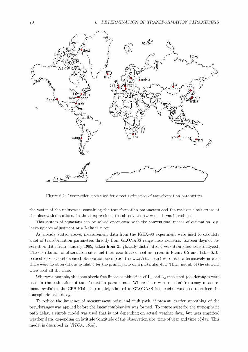
70 6 DETERMINATION OF TRANSFORMATION PARAMETERS
Figure 6.2: Observation sites used for direct estimation of transformation parameters.
the vector of the unknowns, containing the transformation parameters and the receiver clock errors atthe observation stations. In these expressions, the abbreviation ν = n− 1 was introduced.
This system of equations can be solved epoch-wise with the conventional means of estimation, e.g.least-squares adjustment or a Kalman filter.
As already stated above, measurement data from the IGEX-98 experiment were used to calculatea set of transformation parameters directly from GLONASS range measurements. Sixteen days of ob-servation data from January 1999, taken from 21 globally distributed observation sites were analyzed.The distribution of observation sites and their coordinates used are given in Figure 6.2 and Table 6.10,respectively. Closely spaced observation sites (e.g. the wtzg/ntz1 pair) were used alternatively in casethere were no observations available for the primary site on a particular day. Thus, not all of the stationswere used all the time.
Wherever possible, the ionospheric free linear combination of L1 and L2 measured pseudoranges wereused in the estimation of transformation parameters. Where there were no dual-frequency measure-ments available, the GPS Klobuchar model, adapted to GLONASS frequencies, was used to reduce theionospheric path delay.
To reduce the influence of measurement noise and multipath, if present, carrier smoothing of thepseudoranges was applied before the linear combination was formed. To compensate for the troposphericpath delay, a simple model was used that is not depending on actual weather data, but uses empiricalweather data, depending on latitude/longitude of the observation site, time of year and time of day. Thismodel is described in (RTCA, 1998).
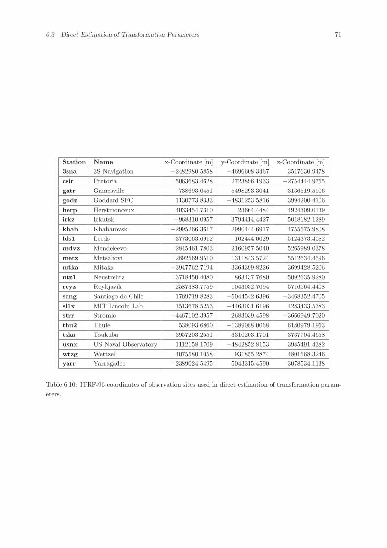
6.3 Direct Estimation of Transformation Parameters 71
Station Name x-Coordinate [m] y-Coordinate [m] z-Coordinate [m]3sna 3S Navigation −2482980.5858 −4696608.3467 3517630.9478csir Pretoria 5063683.4628 2723896.1933 −2754444.9755gatr Gainesville 738693.0451 −5498293.3041 3136519.5906godz Goddard SFC 1130773.8333 −4831253.5816 3994200.4106herp Herstmonceux 4033454.7310 23664.4484 4924309.0139irkz Irkutsk −968310.0957 3794414.4427 5018182.1289khab Khabarovsk −2995266.3617 2990444.6917 4755575.9808lds1 Leeds 3773063.6912 −102444.0029 5124373.4582mdvz Mendeleevo 2845461.7803 2160957.5040 5265989.0378metz Metsahovi 2892569.9510 1311843.5724 5512634.4596mtka Mitaka −3947762.7194 3364399.8226 3699428.5206ntz1 Neustrelitz 3718450.4080 863437.7680 5092635.9280reyz Reykjavik 2587383.7759 −1043032.7094 5716564.4408sang Santiago de Chile 1769719.8283 −5044542.6396 −3468352.4705sl1x MIT Lincoln Lab 1513678.5253 −4463031.6196 4283433.5383strr Stromlo −4467102.3957 2683039.4598 −3666949.7020thu2 Thule 538093.6860 −1389088.0068 6180979.1953tska Tsukuba −3957203.2551 3310203.1701 3737704.4658usnx US Naval Observatory 1112158.1709 −4842852.8153 3985491.4382wtzg Wettzell 4075580.1058 931855.2874 4801568.3246yarr Yarragadee −2389024.5495 5043315.4590 −3078534.1138
Table 6.10: ITRF-96 coordinates of observation sites used in direct estimation of transformation param-eters.
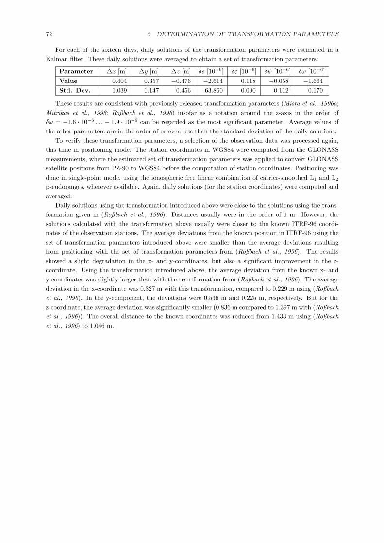
72 6 DETERMINATION OF TRANSFORMATION PARAMETERS
For each of the sixteen days, daily solutions of the transformation parameters were estimated in aKalman filter. These daily solutions were averaged to obtain a set of transformation parameters:
Parameter ∆x [m] ∆y [m] ∆z [m] δs [10−9] δε [10−6] δψ [10−6] δω [10−6]Value 0.404 0.357 −0.476 −2.614 0.118 −0.058 −1.664Std. Dev. 1.039 1.147 0.456 63.860 0.090 0.112 0.170
These results are consistent with previously released transformation parameters (Misra et al., 1996a;Mitrikas et al., 1998; Roßbach et al., 1996) insofar as a rotation around the z-axis in the order ofδω = −1.6 · 10−6 . . . − 1.9 · 10−6 can be regarded as the most significant parameter. Average values ofthe other parameters are in the order of or even less than the standard deviation of the daily solutions.
To verify these transformation parameters, a selection of the observation data was processed again,this time in positioning mode. The station coordinates in WGS84 were computed from the GLONASSmeasurements, where the estimated set of transformation parameters was applied to convert GLONASSsatellite positions from PZ-90 to WGS84 before the computation of station coordinates. Positioning wasdone in single-point mode, using the ionospheric free linear combination of carrier-smoothed L1 and L2
pseudoranges, wherever available. Again, daily solutions (for the station coordinates) were computed andaveraged.
Daily solutions using the transformation introduced above were close to the solutions using the trans-formation given in (Roßbach et al., 1996). Distances usually were in the order of 1 m. However, thesolutions calculated with the transformation above usually were closer to the known ITRF-96 coordi-nates of the observation stations. The average deviations from the known position in ITRF-96 using theset of transformation parameters introduced above were smaller than the average deviations resultingfrom positioning with the set of transformation parameters from (Roßbach et al., 1996). The resultsshowed a slight degradation in the x- and y-coordinates, but also a significant improvement in the z-coordinate. Using the transformation introduced above, the average deviation from the known x- andy-coordinates was slightly larger than with the transformation from (Roßbach et al., 1996). The averagedeviation in the x-coordinate was 0.327 m with this transformation, compared to 0.229 m using (Roßbachet al., 1996). In the y-component, the deviations were 0.536 m and 0.225 m, respectively. But for thez-coordinate, the average deviation was significantly smaller (0.836 m compared to 1.397 m with (Roßbachet al., 1996)). The overall distance to the known coordinates was reduced from 1.433 m using (Roßbachet al., 1996) to 1.046 m.
73
7 Satellite Clock and Orbit Determination
7.1 Satellite Clock Offset
The first step towards the computation of the user’s position always is the determination of the timeof signal transmission. A GLONASS (or GPS) receiver correlates the incoming satellite signal with aninternally created signal, thus determining the signal travel time. The signal travel time, multiplied bythe speed of signal propagation (speed of light in vacuum) then yields the measured (pseudo-)range tothis satellite, which is output by the receiver as an observable.
Given the time of signal reception in a receiver and the signal travel time (or pseudorange), the timeof signal transmission at the satellite can then be determined as
tTX = tRX −∆ttr = tRX − PR/c (7.1.1)
with
tTX Time of signal transmission at satellitetRX Time of signal reception at receiver∆ttr Signal travel timePR Measured pseudorangec Speed of light in vacuum
The time of signal reception is read by the receiver from its own clock and thus is given in the receivertime frame. Signal generation in the satellite is governed by the satellite clock, running in its own timeframe. Therefore, the measured signal travel time is only an approximation of the true signal travel time.That’s why the range derived from the measurement of the signal travel time is called ”pseudo”-range.
To eliminate the effects of different time frames, a unique time frame has to be employed – GLONASSsystem time. GLONASS ephemerides contain parameters to determine the offset of the time frame of thetransmitting satellite to system time (ICD-GLONASS, 1995; ICD-GLONASS, 1998). These parametersare the time scale offset to system time τ and the relative difference of the frequency to the nominal fre-quency γ = (f − fnom) /fnom. Applying these parameters, GLONASS system time tSys can be computedfrom satellite time tSat using the relation
tSys(tSat) = tSat + τ(tb)− γ(tb) · (t− tb) (7.1.2)
with tb being the reference time of the satellite ephemeris data and t the time, for which GLONASSsystem time is desired, t = tSat. Reference time tb is given in system time scale. Thus, in a strict senset also must be given in system time scale. But when determining the satellite clock offset in a receiveror post-processing software, t is given in satellite time scale. However, differences between clock offsetscomputed with t in system time scale and t in satellite time scale are negligibly small, in the order of10−40 s. Therefore, it is sufficient to use the time in satellite time scale: t = tSat. Eq. (7.1.2) has to beapplied to the observed time of signal transmission.
L1 and L2 signals may be transmitted by the satellite at slightly different instances in time due todifferent hardware delays in the equipment used onboard the satellite. Dual-frequency users thereforemust compute different satellite clock offsets for their L1 and L2 pseudorange measurements. However,this is not taken care of by the GLONASS ICD (ICD-GLONASS, 1995). This definitely is one of theimprovements of the GLONASS-M satellites. In their navigation message, they will include the difference∆τn between the equipment delays in L1 and L2 bands: ∆τn = tf2 − tf1, where tf1 and tf2 are therespective delays (ICD-GLONASS, 1998).
For an L1 pseudorange measurement, GLONASS system time is then still computed according to Eq.(7.1.2), whereas for an L2 pseudorange measurement this inter-frequency bias must be considered:
tSys,L1(tSat) = tSat + τ(tb)− γ(tb) · (t− tb) (7.1.3)
tSys,L2(tSat) = tSys,L1(tSat)−∆τn (7.1.4)
74 7 SATELLITE CLOCK AND ORBIT DETERMINATION
The parameter γ does not only contain the effects of the satellite clock drift, but also all gravitationaland relativistic effects. Therefore, a separate compensation for these effects is not necessary, contrary toGPS.
The offset of the receiver clock with respect to GLONASS system time usually is not known a priori.Therefore, this receiver clock error is treated as an additional unknown, which is to be estimated in thecourse of the position determination. This additional unknown necessitates the observation of a fourthsatellite besides the three measurements required for the x-, y- and z-coordinates of the user position.
7.2 Satellite Orbit Determination
7.2.1 Orbital Force Model
Given the time of signal transmission, the next step is to determine the satellite position at that point oftime.
GLONASS broadcast ephemerides contain the satellite position in PZ-90 at the reference time tb,together with the satellite velocity and its acceleration due to luni-solar attraction. These data usuallyare updated every 30 minutes and refer to the center of this 30 minute interval. To obtain the satelliteposition at an epoch other than this reference time (within the validity period of data), the satellite’sequations of motion have to be integrated, using the given values as initial values.
In compliance with Newton’s laws of motion, the motion of a satellite orbiting the Earth is determinedby the forces acting on that satellite. The primary force acting is that caused by Earth’s gravity fieldpotential. This potential can be expressed as
V =µ
r+ U (7.2.1)
with
V Total gravitational potentialµ Earth’s gravitational constantr Distance of satellite to center of EarthU Non-spherical part of Earth’s gravitational potential
The value for µ is adopted from the PZ-90 reference frame (see Table 3.1). Considering only the sphericalpart of the gravitational potential V = µ/r and neglecting also all non-gravitational forces on the satellite,its motion would be pure Keplerian. But these other forces cannot be neglected, thus the motion of thesatellite deviates from a Kepler ellipse. To compensate for this, GPS ephemerides contain correctionalparameters to be applied to an assumed Keplerian orbit. The designers of the GLONASS system chosea different approach by transmitting in the ephemeris data satellite position, velocity and accelerationvectors and having the user integrate the equations of motion with these vectors as initial values, asstated above.
According to (Heiskanen and Moritz, 1967), expansion of the non-spherical part U of the gravitationalpotential into spherical harmonics gives
U =µ
r
∞∑n=2
n∑m=0
(aE
r
)n
Pnm(cos θ) · (cnm cosmλ + snm sin mλ) (7.2.2)
with
aE Earth’s equatorial radiusr, λ, θ Earth-fixed polar coordinates (radius, longitude, colatitude)n, m Degree and order of spherical harmonic expansionPnm(cos θ) Associated Legendre functionscnm, snm Spherical harmonic coefficients
The value for aE is adopted from the PZ-90 reference frame (see Table 3.1).
7.2 Satellite Orbit Determination 75
Since Earth’s gravitational potential is in first approximation rotationally symmetric, i.e. independentof λ, the zonal harmonics (m = 0 in Eq. (7.2.2)), which cause parts of the gravitational potentialindependent of λ, are much more significant to satellite motion than the tesseral (0 < m < n) and thesectorial (m = n) harmonics. It can therefore be assumed that the influence of tesseral and sectorialharmonics is insignificant over a short time span of orbit integration. Thus, Eq. (7.2.2) can be simplifiedto
U =µ
aE
∞∑n=2
(aE
r
)n+1
cn0 · Pn0(cos θ) (7.2.3)
Besides the gravitational force, other forces are acting on a satellite. (Spilker, 1996) summarizes theapproximate perturbing forces acting on GPS satellites as:
Source Max. perturbing acceleration Max. excursion growth in 1h[m/s2] [m]
Spherical Earth 5.65 · 10−1 —Second zonal harmonic 5.3 · 10−5 300Fourth zonal harmonic 10−7 0.6Gravity anomalies 10−8 0.06Lunar gravity 5.5 · 10−6 40Solar gravity 3 · 10−6 20Solar radiation pressure 10−7 0.6All other forces 10−8 0.06
In first approximation considering the forces acting on a GLONASS satellite as identical to thoseacting on GPS satellites, it can be seen that the second zonal harmonic, resulting from Earth’s oblateness,dominates the perturbing forces. Effects of lunar and solar gravitation are one order of magnitude lessthan the second zonal harmonic, all other terms are negligible against these. Thus, it is justifiable torewrite Eq. (7.2.3) with only the second order term:
U =µa2
E
r3c20 ·
(32
cos2 θ − 12
)(7.2.4)
where the Legendre polynomial P20(cos θ) = 3/2 cos2 θ − 1/2 was substituted. Therewith the totalgravitational potential becomes
V =µ
r+
12
µa2E
r3c20 ·
(3 cos2 θ − 1
)(7.2.5)
The satellite acceleration in Cartesian coordinates ~x due to the gravitational potential is defined as
~x = ∇V (7.2.6)
with its components
~xi =dV
dxi=
∂V
∂r
∂r
∂xi+
∂V
∂λ
∂λ
∂xi+
∂V
∂θ
∂θ
∂xi(7.2.7)
With the partial derivatives
∂V
∂r= − µ
r2− 3
2µa2
E
r4c20 ·
(3 cos2 θ − 1
)
∂V
∂λ= 0
∂V
∂θ= −3
µa2E
r3c20 · cos θ sin θ
and∂r
x=
x
r
∂r
y=
y
r
∂r
z=
z
r∂θ
x=
1sin θ
· xz
r3
∂θ
y=
1sin θ
· yz
r3
∂θ
z= − 1
sin θ· r2 − z2
r3
76 7 SATELLITE CLOCK AND ORBIT DETERMINATION
the satellite acceleration due to the gravitational potential is obtained as
x = − µ
r3· x +
32c20
µa2E
r5· x ·
(1− 5
z2
r2
)
y = − µ
r3· y +
32c20
µa2E
r5· y ·
(1− 5
z2
r2
)(7.2.8)
z = − µ
r3· z +
32c20
µa2E
r5· z ·
(3− 5
z2
r2
)
Assuming the acceleration of the satellite due to lunar and solar gravitation to be constant over ashort time span of integration xLS , yLS , zLS and neglecting all other forces, as stated above, the totalacceleration of a GLONASS satellite can then be written as
x = − µ
r3· x +
32c20
µa2E
r5· x ·
(1− 5
z2
r2
)+ xLS
y = − µ
r3· y +
32c20
µa2E
r5· y ·
(1− 5
z2
r2
)+ yLS (7.2.9)
z = − µ
r3· z +
32c20
µa2E
r5· z ·
(3− 5
z2
r2
)+ zLS
Eq. (7.2.9) is valid only in an inertial system, since Newton’s laws of motion as addressed aboveare only valid in inertial systems. The PZ-90 reference frame of GLONASS, however, is an ECEFsystem, rotating with the Earth. To determine the satellite coordinates in PZ-90, one could integratethe satellite’s equations of motion in the inertial system and then transform the obtained coordinates tothe PZ-90 coordinate system. But it is also possible to rewrite the equations of motion in the ECEFcoordinate system.
The transformation from an inertial system to an Earth-fixed system is performed as a series ofrotations (cf. e.g. (Hofmann-Wellenhof et al., 1993)):
~xEF = RM ·RR ·RN ·RP · ~xINS (7.2.10)
with
~xINS Coordinates in inertial system~xEF Coordinates in ECEF systemRM Rotation matrix representing polar motionRR Rotation matrix representing Earth rotationRN Rotation matrix representing nutation of EarthRP Rotation matrix representing precession of Earth
Polar motion, nutation and precession of Earth are very slow processes, with large time constants. Soover a small integration interval, they will not significantly contribute to the deviation of the Earth-fixedsystem from the inertial system. Only Earth rotation, which takes place around the z-axis of the ECEFframe (see definition of the PZ-90 frame), will contribute to this. Accounting for the Coriolis forcescaused by this rotation, the satellite’s equations of motion finally can be written as
dx
dt= x
dy
dt= y
dz
dt= z
dx
dt= − µ
r3· x +
32c20
µa2E
r5· x ·
(1− 5
z2
r2
)+ xLS + ω2
E · x + 2ωE · y (7.2.11)
dy
dt= − µ
r3· y +
32c20
µa2E
r5· y ·
(1− 5
z2
r2
)+ yLS + ω2
E · y − 2ωE · x
dz
dt= − µ
r3· z +
32c20
µa2E
r5· z ·
(3− 5
z2
r2
)+ zLS
7.2 Satellite Orbit Determination 77
with
x, y, z Satellite coordinatesx, y, z Satellite velocitiesxLS , yLS , zLS Luni-solar accelerationr =
√x2 + y2 + z2 Distance of satellite to center of Earth
µ = 3.9860044 · 1014 m3/s2 Earth’s gravitational constantc20 = −1.08263 · 10−3 Second zonal coefficientaE = 6378136 m Earth’s equatorial radiusωE = 7.292115 · 10−5 s−1 Earth’s rotation rate
This is also the way the GLONASS ICD (ICD-GLONASS, 1995) formulates the equations of motion.To obtain the satellite position at a specified time, these equations have to be integrated. To accomplishthis, GLONASS satellites in their ephemeris data transmit the satellite coordinates x, y, z, velocitiesx, y, z and luni-solar acceleration xLS , yLS , zLS at the reference time tb. These values are then usedas initial values in the integration of Eq. (7.2.11). The values for µ, c20, aE , ωE are adopted from thePZ-90 reference frame (see Table 3.1).
7.2.2 Orbit Integration
Even after applying all the approximations and simplifications introduced above, equations (7.2.11) arestill too complex to solve analytically. Therefore, integration is performed numerically. The GLONASSICD (ICD-GLONASS, 1995) recommends using a four step Runge-Kutta method for the integration.This method can be briefly summarized as the following (Jeltsch, 1987):
Given a system of differential equations ~X = ~f(t, ~X) with the initial values ~X0 = ~X(t0), system state~Xn+1 = ~X(tn+1) can be computed numerically from state ~Xn = ~X(tn) using the scheme
~Xn+1 = ~Xn +h
6·[~f(tn, ~Y1) + 2~f(tn +
h
2, ~Y2) + 2~f(tn +
h
2, ~Y3) + ~f(tn + h, ~Y4)
]
~Y1 = ~Xn
~Y2 = ~Xn +h
2~f(tn, ~Y1) (7.2.12)
~Y3 = ~Xn +h
2~f(tn +
h
2, ~Y2)
~Y4 = ~Xn + h~f(tn +h
2, ~Y3)
with h = tn+1 − tn being the step width of the integration.Denoting the vector of the requested orbit parameters (x, y, z, x, y, z)T as the state vector ~X – and
therewith (x, y, z, x, y, z)T as ~X –, system (7.2.11) is already given in the form ~X = ~f(t, ~X) with no
explicit dependence on t: ~X = ~f( ~X). Thus, the scheme of Eq. (7.2.12) simplifies to
~Xn+1 = ~Xn +h
6·[~f(~Y1) + 2~f(~Y2) + 2~f(~Y3) + ~f(~Y4)
]= ~Xn +
h
6·[~D1 + 2 ~D2 + 2 ~D3 + ~D4
]
~Y1 = ~Xn
~Y2 = ~Xn +h
2~f(~Y1)= ~Xn +
h
2~D1 (7.2.13)
~Y3 = ~Xn +h
2~f(~Y2)= ~Xn +
h
2~D2
~Y4 = ~Xn + h~f(~Y3)= ~Xn + h~D3
with ~Di = ~f(~Yi) = ~Y i being the derivatives of the intermediate values. In this form, the scheme of Eq.(7.2.13) can immediately be applied to the equations of motion Eq. (7.2.11):
1. Compute ~D1 = ~f( ~Xn)
78 7 SATELLITE CLOCK AND ORBIT DETERMINATION
2. Compute ~D2 = ~f( ~Xn +h
2~D1)
3. Compute ~D3 = ~f( ~Xn +h
2~D2)
4. Compute ~D4 = ~f( ~Xn + h~D3)
5. Compute ~Xn+1 = ~Xn +h
6
(~D1 + 2 ~D2 + 2 ~D3 + ~D4
)
To determine the position of a GLONASS satellite at time t with the position at the reference time~X0 = ~X(t0 = tb) given, this scheme has to be repeated for t1 = t0 + h, t2 = t1 + h, . . . , until epoch tm
is reached with tm ≤ t < tm + h (respectively tm + h < t ≤ tm, if t < tb, in which case h is negative). Iftm 6= t, a final step has to be performed from epoch tm to t with step width h = t− tm.
It should be noted that according to the GLONASS ICD (ICD-GLONASS, 1995), the parametersfrom the navigation message describe the orbital motion of the satellite’s antenna phase center. Thus,the resulting position vector also defines the coordinates of the phase center and may directly be used inpositioning applications.
According to (Habrich, 1999), however, it must be concluded that the parameters from the GLONASSnavigation message actually describe the orbital motion of the satellite’s center of mass. When beingused in positioning applications, the resulting position and velocity vectors must first be reduced to thepoint of the antenna phase center. Due to the fact that both the center of mass and the phase center arelocated on the satellite x- (longitudinal) axis, and the transmission antenna always points to the Earth,this reduction is a merely radial one. The distance between the phase center and the center of mass isspecified to be 1.62 m. The satellite state vector has to be diminished by that value in radial direction,which is equivalent to a scaling of the vector:
~XPC =
∣∣∣ ~XCM
∣∣∣− 1.62 m∣∣∣ ~XCM
∣∣∣· ~XCM (7.2.14)
with ~XCM being the state (position and velocity) vector of the satellite’s center of mass as computedabove, and ~XPC that of the phase center.
This uncertainty between center of mass and antenna phase center in the satellite ephemerides maybe considered as orbital error, which cancels out in differential operation over short baselines.
7.2.3 Integration Error
When implementing this scheme and determining the satellite position numerically, the obtained satelliteposition and velocity will be depending on the chosen integration step width h. It can be expectedthat the smaller the step width the more accurate the obtained positions will be. On the other hand,the smaller the step width the more integration steps are necessary to obtain the satellite position ata specified epoch in time, increasing the computational load in position determination. After all, ineach integration step function (7.2.11) has to be evaluated four times. Thus, for practical applicationsin positioning, a compromise has to be found for the step width h to allow both satellite positions asaccurate as possible and acceptable computation time, especially in real-time applications.
To assess the influence of the step width on the accuracy of the calculated satellite position, satellitepositions at the midpoint between two validity periods of adjacent ephemeris data were determined usingthese different data sets and varying step widths. In addition, satellite positions at the reference epochof one ephemeris data set were calculated using the other data set. This way, only one of the calculatedsatellite positions was affected by inaccuracies of the numerical integration, while the other positioncould serve as true reference. These calculations were performed in both forward (satellite position atreference epoch of following ephemerides) and backward (satellite position at reference epoch of precedingephemerides) direction. Figure 7.1 illustrates this procedure.
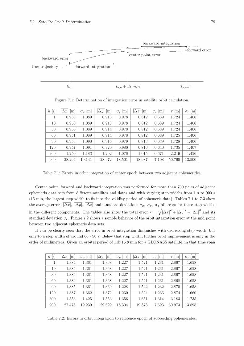
7.2 Satellite Orbit Determination 79
tb,n tb,n + 15 min tb,n+1
r
r
true trajectory-
forward integration
¾backward integration
6
?backward error
6
?
center point error6?forward error
Figure 7.1: Determination of integration error in satellite orbit calculation.
h [s] |∆x| [m] σx [m] |∆y| [m] σy [m] |∆z| [m] σz [m] r [m] σr [m]1 0.950 1.089 0.913 0.978 0.812 0.639 1.724 1.406
10 0.950 1.089 0.913 0.978 0.812 0.639 1.724 1.40630 0.950 1.089 0.914 0.978 0.812 0.639 1.724 1.40660 0.951 1.089 0.914 0.978 0.812 0.639 1.725 1.40690 0.953 1.090 0.916 0.979 0.813 0.639 1.728 1.406
120 0.957 1.091 0.920 0.980 0.816 0.640 1.735 1.407300 1.250 1.183 1.202 1.076 1.015 0.671 2.219 1.456900 28.294 19.141 28.972 18.501 18.987 7.108 50.760 13.500
Table 7.1: Errors in orbit integration of center epoch between two adjacent ephemerides.
Center point, forward and backward integration was performed for more than 700 pairs of adjacentephemeris data sets from different satellites and dates and with varying step widths from 1 s to 900 s(15 min, the largest step width to fit into the validity period of ephemeris data). Tables 7.1 to 7.3 showthe average errors |∆x|, |∆y|, |∆z| and standard deviations σx, σy, σz of errors for these step widths
in the different components. The tables also show the total error r =√|∆x|2 + |∆y|2 + |∆z|2 and its
standard deviation σr. Figure 7.2 shows a sample behavior of the orbit integration error at the mid pointbetween two adjacent ephemeris data sets.
It can be clearly seen that the error in orbit integration diminishes with decreasing step width, butonly to a step width of around 60 - 90 s. Below that step width, further orbit improvement is only in theorder of millimeters. Given an orbital period of 11h 15.8 min for a GLONASS satellite, in that time span
h [s] |∆x| [m] σx [m] |∆y| [m] σy [m] |∆z| [m] σz [m] r [m] σr [m]1 1.384 1.361 1.368 1.227 1.521 1.231 2.867 1.658
10 1.384 1.361 1.368 1.227 1.521 1.231 2.867 1.65830 1.384 1.361 1.368 1.227 1.521 1.231 2.867 1.65860 1.384 1.361 1.368 1.227 1.521 1.231 2.868 1.65890 1.385 1.361 1.369 1.228 1.522 1.232 2.870 1.658
120 1.387 1.362 1.372 1.230 1.524 1.233 2.874 1.660300 1.553 1.425 1.553 1.356 1.651 1.314 3.183 1.735900 27.478 19.239 29.629 18.304 19.873 7.693 50.973 13.898
Table 7.2: Errors in orbit integration to reference epoch of succeeding ephemerides.
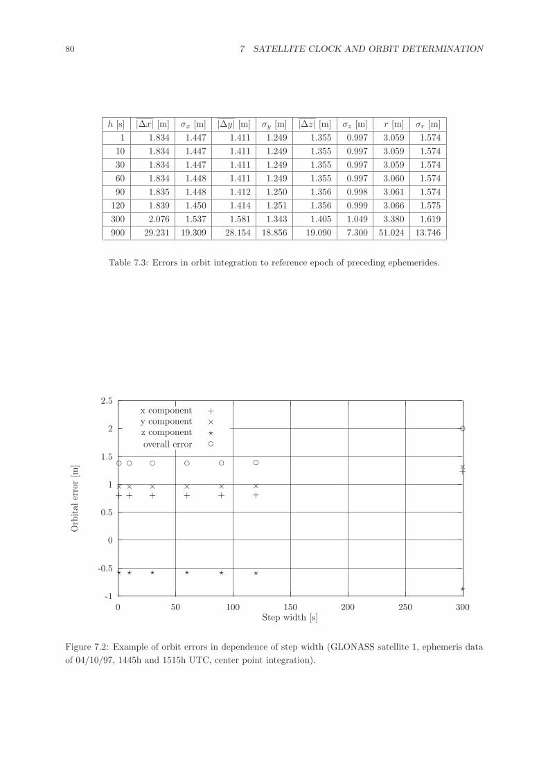
80 7 SATELLITE CLOCK AND ORBIT DETERMINATION
h [s] |∆x| [m] σx [m] |∆y| [m] σy [m] |∆z| [m] σz [m] r [m] σr [m]1 1.834 1.447 1.411 1.249 1.355 0.997 3.059 1.574
10 1.834 1.447 1.411 1.249 1.355 0.997 3.059 1.57430 1.834 1.447 1.411 1.249 1.355 0.997 3.059 1.57460 1.834 1.448 1.411 1.249 1.355 0.997 3.060 1.57490 1.835 1.448 1.412 1.250 1.356 0.998 3.061 1.574
120 1.839 1.450 1.414 1.251 1.356 0.999 3.066 1.575300 2.076 1.537 1.581 1.343 1.405 1.049 3.380 1.619900 29.231 19.309 28.154 18.856 19.090 7.300 51.024 13.746
Table 7.3: Errors in orbit integration to reference epoch of preceding ephemerides.
-1
-0.5
0
0.5
1
1.5
2
2.5
0 50 100 150 200 250 300
Orb
ital
erro
r[m
]
Step width [s]
x component
+ + + + + +
+
+y component
× × × × × ××
×z component
? ? ? ? ? ?
?
?
overall error
d d d d d d
dd
Figure 7.2: Example of orbit errors in dependence of step width (GLONASS satellite 1, ephemeris dataof 04/10/97, 1445h and 1515h UTC, center point integration).
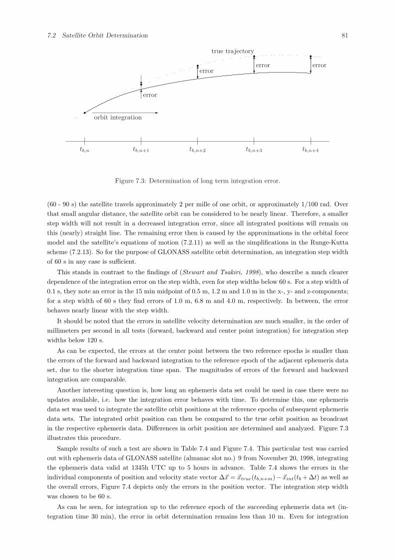
7.2 Satellite Orbit Determination 81
tb,n tb,n+1 tb,n+2 tb,n+3 tb,n+4
r
r
rr rtrue trajectory
-orbit integration
6
?
error
6?error
6
?error
6
?error
Figure 7.3: Determination of long term integration error.
(60 - 90 s) the satellite travels approximately 2 per mille of one orbit, or approximately 1/100 rad. Overthat small angular distance, the satellite orbit can be considered to be nearly linear. Therefore, a smallerstep width will not result in a decreased integration error, since all integrated positions will remain onthis (nearly) straight line. The remaining error then is caused by the approximations in the orbital forcemodel and the satellite’s equations of motion (7.2.11) as well as the simplifications in the Runge-Kuttascheme (7.2.13). So for the purpose of GLONASS satellite orbit determination, an integration step widthof 60 s in any case is sufficient.
This stands in contrast to the findings of (Stewart and Tsakiri, 1998), who describe a much clearerdependence of the integration error on the step width, even for step widths below 60 s. For a step width of0.1 s, they note an error in the 15 min midpoint of 0.5 m, 1.2 m and 1.0 m in the x-, y- and z-components;for a step width of 60 s they find errors of 1.0 m, 6.8 m and 4.0 m, respectively. In between, the errorbehaves nearly linear with the step width.
It should be noted that the errors in satellite velocity determination are much smaller, in the order ofmillimeters per second in all tests (forward, backward and center point integration) for integration stepwidths below 120 s.
As can be expected, the errors at the center point between the two reference epochs is smaller thanthe errors of the forward and backward integration to the reference epoch of the adjacent ephemeris dataset, due to the shorter integration time span. The magnitudes of errors of the forward and backwardintegration are comparable.
Another interesting question is, how long an ephemeris data set could be used in case there were noupdates available, i.e. how the integration error behaves with time. To determine this, one ephemerisdata set was used to integrate the satellite orbit positions at the reference epochs of subsequent ephemerisdata sets. The integrated orbit position can then be compared to the true orbit position as broadcastin the respective ephemeris data. Differences in orbit position are determined and analyzed. Figure 7.3illustrates this procedure.
Sample results of such a test are shown in Table 7.4 and Figure 7.4. This particular test was carriedout with ephemeris data of GLONASS satellite (almanac slot no.) 9 from November 20, 1998, integratingthe ephemeris data valid at 1345h UTC up to 5 hours in advance. Table 7.4 shows the errors in theindividual components of position and velocity state vector ∆~x = ~xtrue(tb,n+m)−~xint(tb +∆t) as well asthe overall errors, Figure 7.4 depicts only the errors in the position vector. The integration step widthwas chosen to be 60 s.
As can be seen, for integration up to the reference epoch of the succeeding ephemeris data set (in-tegration time 30 min), the error in orbit determination remains less than 10 m. Even for integration
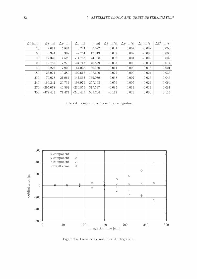
82 7 SATELLITE CLOCK AND ORBIT DETERMINATION
∆t [min] ∆x [m] ∆y [m] ∆z [m] r [m] ∆x [m/s] ∆y [m/s] ∆z [m/s] ∆|~x| [m/s]30 2.071 5.884 3.224 7.022 0.001 0.002 -0.002 0.00360 6.974 10.397 -2.754 12.819 0.002 0.002 -0.005 0.00690 12.340 14.523 -14.763 24.108 0.002 0.001 -0.009 0.009
120 12.785 17.278 -34.713 40.829 -0.003 0.000 -0.014 0.014150 2.276 17.929 -64.028 66.530 -0.011 0.000 -0.018 0.021180 -25.921 19.380 -102.617 107.600 -0.022 -0.000 -0.024 0.033210 -79.028 21.964 -147.863 169.089 -0.038 0.002 -0.026 0.046240 -166.242 29.734 -193.979 257.193 -0.059 0.005 -0.024 0.064270 -295.078 46.562 -230.859 377.537 -0.085 0.013 -0.014 0.087300 -472.433 77.474 -240.449 535.734 -0.112 0.023 0.006 0.114
Table 7.4: Long-term errors in orbit integration.
-600
-400
-200
0
200
400
600
0 50 100 150 200 250 300
Orb
ital
erro
r[m
]
Integration time [min]
x component
+ + + + + ++
+
+
+
+y component
× × × × × × × × × ×
×z component
? ? ? ??
??
?? ?
?
overall error
d d d d d dd
d
d
d
d
Figure 7.4: Long-term errors in orbit integration.
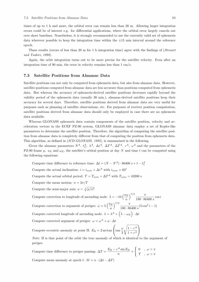
7.3 Satellite Positions from Almanac Data 83
times of up to 1 h and more, the orbital error can remain less than 20 m. Allowing larger integrationerrors could be of interest e.g. for differential applications, where the orbital error largely cancels outover short baselines. Nonetheless, it is strongly recommended to use the currently valid set of ephemerisdata wherever possible to keep the integration time within the ±15 min interval around the referenceepoch.
These results (errors of less than 20 m for 1 h integration time) agree with the findings of (Stewartand Tsakiri, 1998).
Again, the orbit integration turns out to be more precise for the satellite velocity. Even after anintegration time of 90 min, the error in velocity remains less than 1 cm/s.
7.3 Satellite Positions from Almanac Data
Satellite positions can not only be computed from ephemeris data, but also from almanac data. However,satellite positions computed from almanac data are less accurate than positions computed from ephemerisdata. But whereas the accuracy of ephemeris-derived satellite positions decreases rapidly beyond thevalidity period of the ephemeris data (usually 30 min.), almanac-derived satellite positions keep theiraccuracy for several days. Therefore, satellite positions derived from almanac data are very useful forpurposes such as planning of satellite observations, etc. For purposes of receiver position computation,satellite positions derived from almanac data should only be employed in case there are no ephemerisdata available.
Whereas GLONASS ephemeris data contain components of the satellite position, velocity and ac-celeration vectors in the ECEF PZ-90 system, GLONASS almanac data employ a set of Kepler-likeparameters to determine the satellite position. Therefore, the algorithm of computing the satellite posi-tion from almanac data is completely different from that of computing the position from ephemeris data.This algorithm, as defined in (ICD-GLONASS, 1995), is summarized in the following.
Given the almanac parameters NA, tAλ , λA, ∆iA, ∆TA, ∆TA, εA, ωA and the parameters of thePZ-90 frame µ, aE and ωE , the satellite’s orbital position at day N and time t can be computed usingthe following equations:
Compute time difference to reference time: ∆t = (N −NA) · 86400 s + t− tAλ
Compute the actual inclination: i = inom + ∆iA with inom = 63◦
Compute the actual orbital period: T = Tnom + ∆TA with Tnom = 43200 s
Compute the mean motion: n = 2π/T
Compute the semi-major axis: a = 3√
µ/n2
Compute correction to longitude of ascending node: λ = −10(aE
a
)7/2 π
180 · 86400 scos i
Compute correction to argument of perigee: ω = 5(aE
a
)7/2 π
180 · 86400 s(5 cos2 i− 1)
Compute corrected longitude of ascending node: λ = λA +(λ− ωE
)·∆t
Compute corrected argument of perigee: ω = ωA + ω ·∆t
Compute eccentric anomaly at point Π: EΠ = 2 arctan
tan
ω
2
√1− εA
1 + εA
Note: Π is that point of the orbit the true anomaly of which is identical to the argument ofperigee.
Compute time difference to perigee passing: ∆T =EΠ − εA sin EΠ
n+
{0 , ω < π
T , ω > π
Compute mean anomaly at epoch t: M = n · (∆t−∆T )
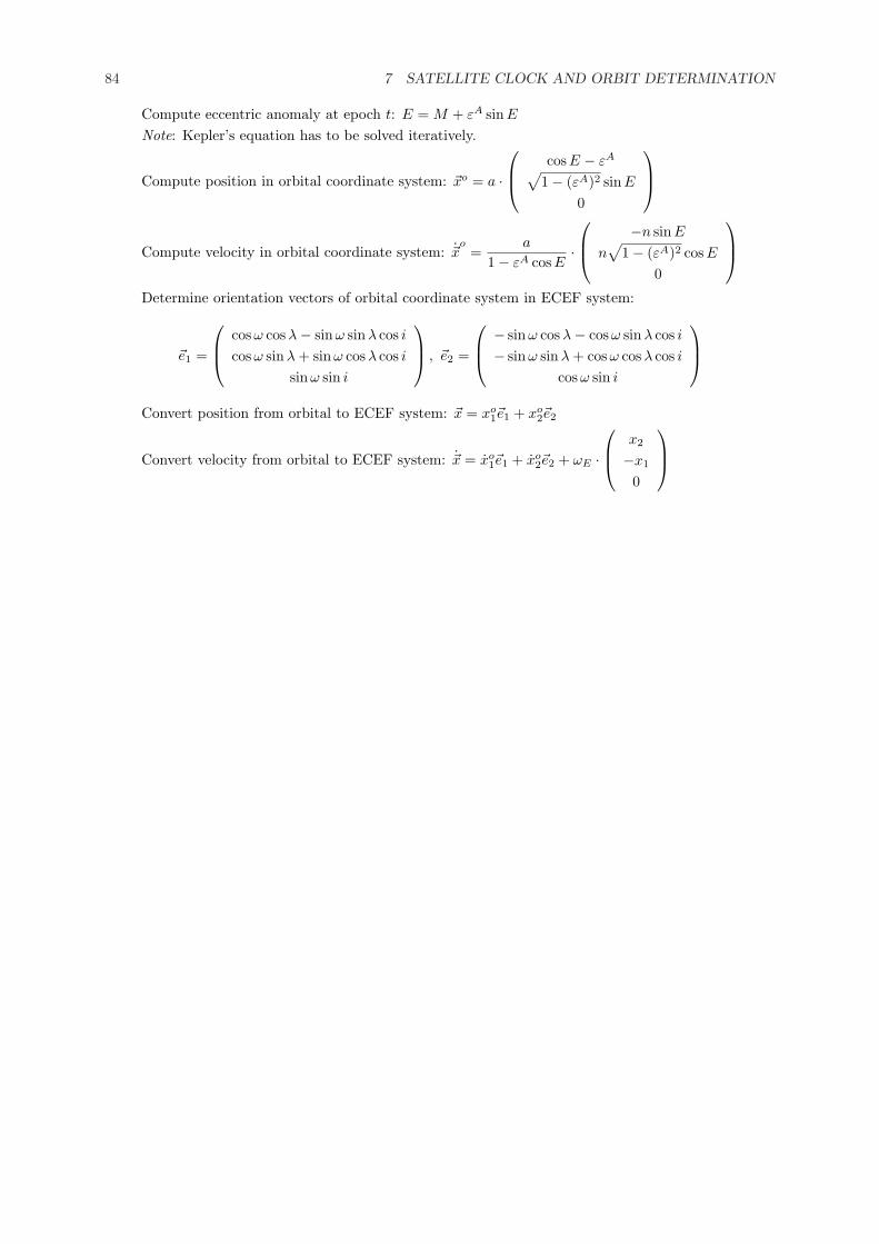
84 7 SATELLITE CLOCK AND ORBIT DETERMINATION
Compute eccentric anomaly at epoch t: E = M + εA sin E
Note: Kepler’s equation has to be solved iteratively.
Compute position in orbital coordinate system: ~xo = a ·
cosE − εA
√1− (εA)2 sin E
0
Compute velocity in orbital coordinate system: ~xo
=a
1− εA cosE·
−n sinE
n√
1− (εA)2 cosE
0
Determine orientation vectors of orbital coordinate system in ECEF system:
~e1 =
cosω cosλ− sin ω sin λ cos i
cosω sin λ + sin ω cosλ cos i
sin ω sin i
, ~e2 =
− sin ω cos λ− cosω sin λ cos i
− sin ω sin λ + cos ω cos λ cos i
cosω sin i
Convert position from orbital to ECEF system: ~x = xo1~e1 + xo
2~e2
Convert velocity from orbital to ECEF system: ~x = xo1~e1 + xo
2~e2 + ωE ·
x2
−x1
0
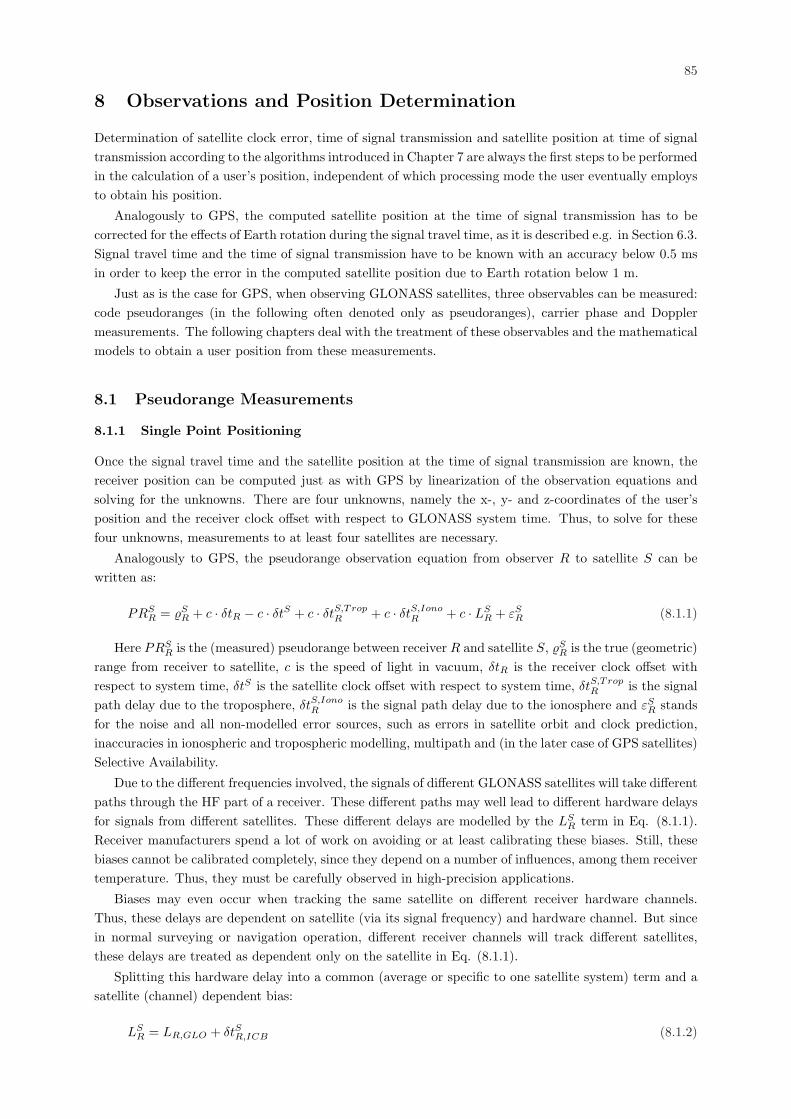
85
8 Observations and Position Determination
Determination of satellite clock error, time of signal transmission and satellite position at time of signaltransmission according to the algorithms introduced in Chapter 7 are always the first steps to be performedin the calculation of a user’s position, independent of which processing mode the user eventually employsto obtain his position.
Analogously to GPS, the computed satellite position at the time of signal transmission has to becorrected for the effects of Earth rotation during the signal travel time, as it is described e.g. in Section 6.3.Signal travel time and the time of signal transmission have to be known with an accuracy below 0.5 msin order to keep the error in the computed satellite position due to Earth rotation below 1 m.
Just as is the case for GPS, when observing GLONASS satellites, three observables can be measured:code pseudoranges (in the following often denoted only as pseudoranges), carrier phase and Dopplermeasurements. The following chapters deal with the treatment of these observables and the mathematicalmodels to obtain a user position from these measurements.
8.1 Pseudorange Measurements
8.1.1 Single Point Positioning
Once the signal travel time and the satellite position at the time of signal transmission are known, thereceiver position can be computed just as with GPS by linearization of the observation equations andsolving for the unknowns. There are four unknowns, namely the x-, y- and z-coordinates of the user’sposition and the receiver clock offset with respect to GLONASS system time. Thus, to solve for thesefour unknowns, measurements to at least four satellites are necessary.
Analogously to GPS, the pseudorange observation equation from observer R to satellite S can bewritten as:
PRSR = %S
R + c · δtR − c · δtS + c · δtS,TropR + c · δtS,Iono
R + c · LSR + εS
R (8.1.1)
Here PRSR is the (measured) pseudorange between receiver R and satellite S, %S
R is the true (geometric)range from receiver to satellite, c is the speed of light in vacuum, δtR is the receiver clock offset withrespect to system time, δtS is the satellite clock offset with respect to system time, δtS,Trop
R is the signalpath delay due to the troposphere, δtS,Iono
R is the signal path delay due to the ionosphere and εSR stands
for the noise and all non-modelled error sources, such as errors in satellite orbit and clock prediction,inaccuracies in ionospheric and tropospheric modelling, multipath and (in the later case of GPS satellites)Selective Availability.
Due to the different frequencies involved, the signals of different GLONASS satellites will take differentpaths through the HF part of a receiver. These different paths may well lead to different hardware delaysfor signals from different satellites. These different delays are modelled by the LS
R term in Eq. (8.1.1).Receiver manufacturers spend a lot of work on avoiding or at least calibrating these biases. Still, thesebiases cannot be calibrated completely, since they depend on a number of influences, among them receivertemperature. Thus, they must be carefully observed in high-precision applications.
Biases may even occur when tracking the same satellite on different receiver hardware channels.Thus, these delays are dependent on satellite (via its signal frequency) and hardware channel. But sincein normal surveying or navigation operation, different receiver channels will track different satellites,these delays are treated as dependent only on the satellite in Eq. (8.1.1).
Splitting this hardware delay into a common (average or specific to one satellite system) term and asatellite (channel) dependent bias:
LSR = LR,GLO + δtSR,ICB (8.1.2)
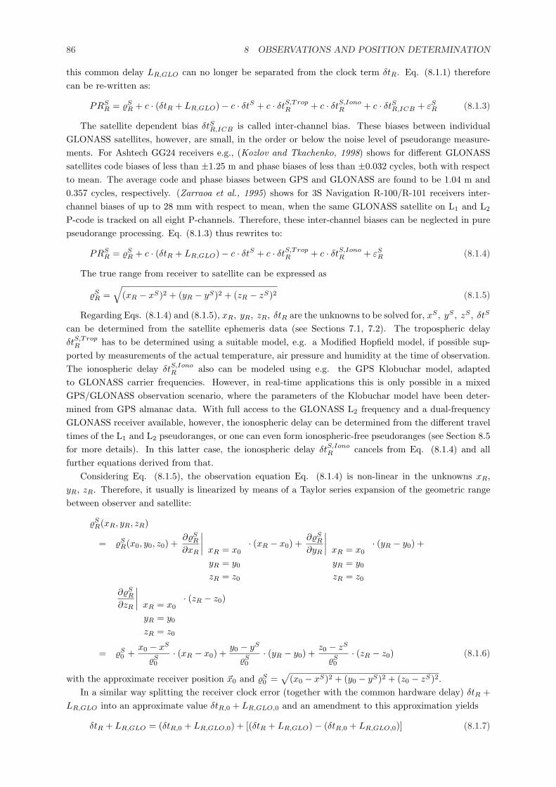
86 8 OBSERVATIONS AND POSITION DETERMINATION
this common delay LR,GLO can no longer be separated from the clock term δtR. Eq. (8.1.1) thereforecan be re-written as:
PRSR = %S
R + c · (δtR + LR,GLO)− c · δtS + c · δtS,TropR + c · δtS,Iono
R + c · δtSR,ICB + εSR (8.1.3)
The satellite dependent bias δtSR,ICB is called inter-channel bias. These biases between individualGLONASS satellites, however, are small, in the order or below the noise level of pseudorange measure-ments. For Ashtech GG24 receivers e.g., (Kozlov and Tkachenko, 1998) shows for different GLONASSsatellites code biases of less than ±1.25 m and phase biases of less than ±0.032 cycles, both with respectto mean. The average code and phase biases between GPS and GLONASS are found to be 1.04 m and0.357 cycles, respectively. (Zarraoa et al., 1995) shows for 3S Navigation R-100/R-101 receivers inter-channel biases of up to 28 mm with respect to mean, when the same GLONASS satellite on L1 and L2
P-code is tracked on all eight P-channels. Therefore, these inter-channel biases can be neglected in purepseudorange processing. Eq. (8.1.3) thus rewrites to:
PRSR = %S
R + c · (δtR + LR,GLO)− c · δtS + c · δtS,TropR + c · δtS,Iono
R + εSR (8.1.4)
The true range from receiver to satellite can be expressed as
%SR =
√(xR − xS)2 + (yR − yS)2 + (zR − zS)2 (8.1.5)
Regarding Eqs. (8.1.4) and (8.1.5), xR, yR, zR, δtR are the unknowns to be solved for, xS , yS , zS , δtS
can be determined from the satellite ephemeris data (see Sections 7.1, 7.2). The tropospheric delayδtS,Trop
R has to be determined using a suitable model, e.g. a Modified Hopfield model, if possible sup-ported by measurements of the actual temperature, air pressure and humidity at the time of observation.The ionospheric delay δtS,Iono
R also can be modeled using e.g. the GPS Klobuchar model, adaptedto GLONASS carrier frequencies. However, in real-time applications this is only possible in a mixedGPS/GLONASS observation scenario, where the parameters of the Klobuchar model have been deter-mined from GPS almanac data. With full access to the GLONASS L2 frequency and a dual-frequencyGLONASS receiver available, however, the ionospheric delay can be determined from the different traveltimes of the L1 and L2 pseudoranges, or one can even form ionospheric-free pseudoranges (see Section 8.5for more details). In this latter case, the ionospheric delay δtS,Iono
R cancels from Eq. (8.1.4) and allfurther equations derived from that.
Considering Eq. (8.1.5), the observation equation Eq. (8.1.4) is non-linear in the unknowns xR,yR, zR. Therefore, it usually is linearized by means of a Taylor series expansion of the geometric rangebetween observer and satellite:
%SR(xR, yR, zR)
= %SR(x0, y0, z0) +
∂%SR
∂xR
∣∣∣∣ xR = x0
yR = y0
zR = z0
· (xR − x0) +∂%S
R
∂yR
∣∣∣∣ xR = x0
yR = y0
zR = z0
· (yR − y0) +
∂%SR
∂zR
∣∣∣∣ xR = x0
yR = y0
zR = z0
· (zR − z0)
= %S0 +
x0 − xS
%S0
· (xR − x0) +y0 − yS
%S0
· (yR − y0) +z0 − zS
%S0
· (zR − z0) (8.1.6)
with the approximate receiver position ~x0 and %S0 =
√(x0 − xS)2 + (y0 − yS)2 + (z0 − zS)2.
In a similar way splitting the receiver clock error (together with the common hardware delay) δtR +LR,GLO into an approximate value δtR,0 + LR,GLO,0 and an amendment to this approximation yields
δtR + LR,GLO = (δtR,0 + LR,GLO,0) + [(δtR + LR,GLO)− (δtR,0 + LR,GLO,0)] (8.1.7)
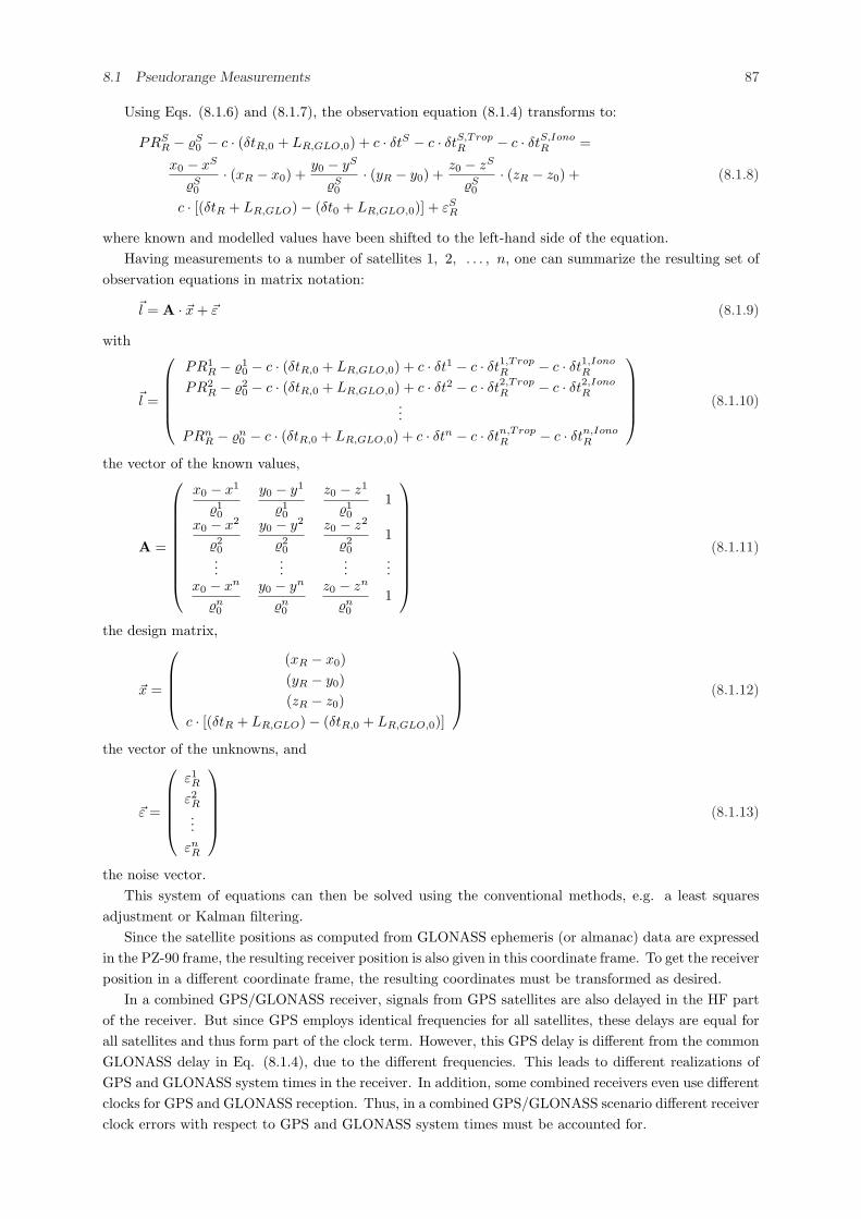
8.1 Pseudorange Measurements 87
Using Eqs. (8.1.6) and (8.1.7), the observation equation (8.1.4) transforms to:
PRSR − %S
0 − c · (δtR,0 + LR,GLO,0) + c · δtS − c · δtS,TropR − c · δtS,Iono
R =
x0 − xS
%S0
· (xR − x0) +y0 − yS
%S0
· (yR − y0) +z0 − zS
%S0
· (zR − z0) + (8.1.8)
c · [(δtR + LR,GLO)− (δt0 + LR,GLO,0)] + εSR
where known and modelled values have been shifted to the left-hand side of the equation.Having measurements to a number of satellites 1, 2, . . . , n, one can summarize the resulting set of
observation equations in matrix notation:
~l = A · ~x + ~ε (8.1.9)
with
~l =
PR1R − %1
0 − c · (δtR,0 + LR,GLO,0) + c · δt1 − c · δt1,TropR − c · δt1,Iono
R
PR2R − %2
0 − c · (δtR,0 + LR,GLO,0) + c · δt2 − c · δt2,TropR − c · δt2,Iono
R...
PRnR − %n
0 − c · (δtR,0 + LR,GLO,0) + c · δtn − c · δtn,TropR − c · δtn,Iono
R
(8.1.10)
the vector of the known values,
A =
x0 − x1
%10
y0 − y1
%10
z0 − z1
%10
1
x0 − x2
%20
y0 − y2
%20
z0 − z2
%20
1
......
......
x0 − xn
%n0
y0 − yn
%n0
z0 − zn
%n0
1
(8.1.11)
the design matrix,
~x =
(xR − x0)(yR − y0)(zR − z0)
c · [(δtR + LR,GLO)− (δtR,0 + LR,GLO,0)]
(8.1.12)
the vector of the unknowns, and
~ε =
ε1R
ε2R...
εnR
(8.1.13)
the noise vector.This system of equations can then be solved using the conventional methods, e.g. a least squares
adjustment or Kalman filtering.Since the satellite positions as computed from GLONASS ephemeris (or almanac) data are expressed
in the PZ-90 frame, the resulting receiver position is also given in this coordinate frame. To get the receiverposition in a different coordinate frame, the resulting coordinates must be transformed as desired.
In a combined GPS/GLONASS receiver, signals from GPS satellites are also delayed in the HF partof the receiver. But since GPS employs identical frequencies for all satellites, these delays are equal forall satellites and thus form part of the clock term. However, this GPS delay is different from the commonGLONASS delay in Eq. (8.1.4), due to the different frequencies. This leads to different realizations ofGPS and GLONASS system times in the receiver. In addition, some combined receivers even use differentclocks for GPS and GLONASS reception. Thus, in a combined GPS/GLONASS scenario different receiverclock errors with respect to GPS and GLONASS system times must be accounted for.
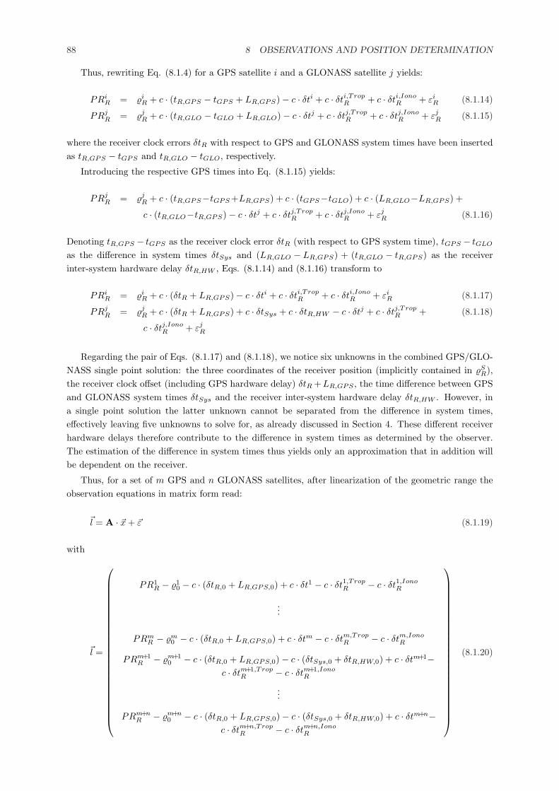
88 8 OBSERVATIONS AND POSITION DETERMINATION
Thus, rewriting Eq. (8.1.4) for a GPS satellite i and a GLONASS satellite j yields:
PRiR = %i
R + c · (tR,GPS − tGPS + LR,GPS)− c · δti + c · δti,TropR + c · δti,Iono
R + εiR (8.1.14)
PRjR = %j
R + c · (tR,GLO − tGLO + LR,GLO)− c · δtj + c · δtj,TropR + c · δtj,Iono
R + εjR (8.1.15)
where the receiver clock errors δtR with respect to GPS and GLONASS system times have been insertedas tR,GPS − tGPS and tR,GLO − tGLO, respectively.
Introducing the respective GPS times into Eq. (8.1.15) yields:
PRjR = %j
R + c · (tR,GPS−tGPS +LR,GPS) + c · (tGPS−tGLO) + c · (LR,GLO−LR,GPS) +
c · (tR,GLO−tR,GPS)− c · δtj + c · δtj,TropR + c · δtj,Iono
R + εjR (8.1.16)
Denoting tR,GPS − tGPS as the receiver clock error δtR (with respect to GPS system time), tGPS − tGLO
as the difference in system times δtSys and (LR,GLO − LR,GPS) + (tR,GLO − tR,GPS) as the receiverinter-system hardware delay δtR,HW , Eqs. (8.1.14) and (8.1.16) transform to
PRiR = %i
R + c · (δtR + LR,GPS)− c · δti + c · δti,TropR + c · δti,Iono
R + εiR (8.1.17)
PRjR = %j
R + c · (δtR + LR,GPS) + c · δtSys + c · δtR,HW − c · δtj + c · δtj,TropR + (8.1.18)
c · δtj,IonoR + εj
R
Regarding the pair of Eqs. (8.1.17) and (8.1.18), we notice six unknowns in the combined GPS/GLO-NASS single point solution: the three coordinates of the receiver position (implicitly contained in %S
R),the receiver clock offset (including GPS hardware delay) δtR +LR,GPS , the time difference between GPSand GLONASS system times δtSys and the receiver inter-system hardware delay δtR,HW . However, ina single point solution the latter unknown cannot be separated from the difference in system times,effectively leaving five unknowns to solve for, as already discussed in Section 4. These different receiverhardware delays therefore contribute to the difference in system times as determined by the observer.The estimation of the difference in system times thus yields only an approximation that in addition willbe dependent on the receiver.
Thus, for a set of m GPS and n GLONASS satellites, after linearization of the geometric range theobservation equations in matrix form read:
~l = A · ~x + ~ε (8.1.19)
with
~l =
PR1R − %1
0 − c · (δtR,0 + LR,GPS,0) + c · δt1 − c · δt1,TropR − c · δt1,Iono
R
...
PRmR − %m
0 − c · (δtR,0 + LR,GPS,0) + c · δtm − c · δtm,TropR − c · δtm,Iono
R
PRm+1R − %m+1
0 − c · (δtR,0 + LR,GPS,0)− c · (δtSys,0 + δtR,HW,0) + c · δtm+1−c · δtm+1,Trop
R − c · δtm+1,IonoR
...
PRm+nR − %m+n
0 − c · (δtR,0 + LR,GPS,0)− c · (δtSys,0 + δtR,HW,0) + c · δtm+n−c · δtm+n,Trop
R − c · δtm+n,IonoR
(8.1.20)

8.1 Pseudorange Measurements 89
the vector of the known values,
A =
x0 − x1
%10
y0 − y1
%10
z0 − z1
%10
1 0
......
......
...x0 − xm
%m0
y0 − ym
%m0
z0 − zm
%m0
1 0
x0 − xm+1
%m+10
y0 − ym+1
%m+10
z0 − zm+1
%m+10
1 1
......
......
...x0 − xm+n
%m+n0
y0 − ym+n
%m+n0
z0 − zm+n
%m+n0
1 1
(8.1.21)
the design matrix,
~x =
(xR − x0)(yR − y0)(zR − z0)
c · [(δtR + LR,GPS)− (δtR,0 + LR,GPS,0)]c · [(δtSys + δtR,HW )− (δtSys,0 + δtR,HW,0)]
(8.1.22)
the vector of the unknowns, and
~ε =
ε1R...
εmR
εm+1R...
εm+nR
(8.1.23)
the noise vector.Please note that tR and δtR now denote the receiver clock reading and offset with respect to GPS
system time, as described above.Satellite coordinates ~x1, . . . , ~xm, ~xm+1, . . . , ~xm+n must be given in the same coordinate frame to
obtain a valid receiver position (cf. Section 5). Coordinates of the receiver position are then expressedin the frame used for the satellite positions.
An example of positioning results using GPS and GLONASS absolute positioning with pseudorangesis shown in Figure 8.1. Positions were computed from data logged by a 3S Navigation R-100/R-101receiver, which was set up at a known location at the Institute of Geodesy and Navigation. Pseudorangeand carrier phase measurements were logged every second for approximately one hour. The plot shows thedeviation from the known location of the antenna in the horizontal plane. GPS positions were computedfrom carrier smoothed L1 C/A-code pseudorange measurements. GLONASS positions were computedfrom carrier smoothed dual-frequency P-code measurements. Wherever possible, the ionospheric freelinear combination was formed. These observables used are not really identical for GPS and GLONASS,but with P-code and dual-frequency measurements readily available on GLONASS, the best possibleresults for each system are determined. GLONASS satellite positions were converted from PZ-90 toWGS84 using the transformation according to (Roßbach et al., 1996).
The large deviations from the true position due to GPS S/A can be clearly seen. Standard deviationsof the computed positions are 25.4 m in North/South direction and 10.0 m in East/West direction.Due to the lack of S/A on GLONASS, positions computed only from GLONASS range measurementsscatter much less. Here the standard deviations are 4.6 m in North/South direction and 7.5 m inEast/West direction. For the combined GPS/GLONASS positioning, all satellite measurements were
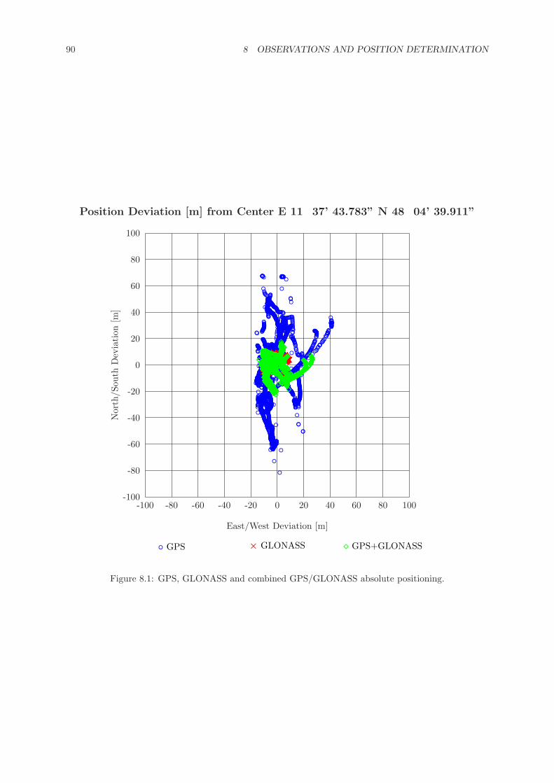
90 8 OBSERVATIONS AND POSITION DETERMINATION
Position Deviation [m] from Center E 11� 37’ 43.783” N 48� 04’ 39.911”
◦ GPS × GLONASS ¦ GPS+GLONASS
East/West Deviation [m]
-100 -80 -60 -40 -20 0 20 40 60 80 100
Nor
th/S
outh
Dev
iati
on[m
]
-100
-80
-60
-40
-20
0
20
40
60
80
100
◦ ◦◦◦◦◦◦◦◦◦◦◦◦◦◦◦ ◦◦◦◦◦◦◦◦◦◦◦◦◦◦◦◦◦◦◦◦◦◦◦◦◦◦◦◦◦◦◦◦◦◦◦◦◦◦◦◦◦◦◦◦◦◦◦◦◦◦◦◦◦◦◦◦◦◦◦◦◦◦◦◦◦◦◦◦◦ ◦◦◦◦◦◦◦◦◦◦◦◦◦◦◦◦◦◦◦◦◦◦◦◦◦◦◦◦◦◦◦◦◦◦◦◦◦◦◦◦◦◦◦◦◦◦◦◦◦◦◦◦◦◦◦◦◦◦◦◦◦◦◦◦◦◦◦◦◦◦◦◦◦◦◦◦◦◦◦◦◦◦◦◦◦◦◦◦◦◦◦◦◦◦◦◦◦◦◦◦◦◦◦◦◦◦◦◦◦◦◦◦◦◦◦◦◦◦◦◦◦◦◦◦◦◦◦◦◦◦◦◦◦◦◦◦◦◦◦◦◦◦◦◦◦◦◦◦
◦◦◦◦◦◦◦◦◦◦◦◦◦◦◦◦◦◦◦◦◦◦◦◦◦◦◦◦◦◦◦◦◦◦◦◦◦◦◦◦◦◦◦◦◦◦◦◦◦◦◦◦◦◦◦◦◦◦◦◦◦◦◦◦◦◦◦◦◦◦◦◦◦◦◦◦◦◦◦◦◦◦◦◦◦◦◦◦◦◦◦◦◦◦◦◦◦◦◦◦◦◦◦◦◦◦◦◦◦◦◦◦◦◦◦◦◦◦◦◦◦◦◦◦◦◦◦◦◦◦◦◦◦◦◦◦◦◦◦◦◦◦◦◦◦◦◦◦◦◦◦◦◦◦◦◦◦◦◦◦◦◦◦◦◦◦◦◦◦◦◦◦◦
◦
◦◦◦◦◦◦◦◦◦◦◦◦◦◦◦◦◦◦◦◦◦◦◦◦◦◦◦◦◦◦◦◦◦◦◦◦◦◦◦◦◦◦◦◦◦◦◦◦◦◦◦◦◦◦◦◦◦◦◦◦◦◦◦◦◦
◦
◦◦◦◦◦◦◦◦◦◦◦◦◦◦◦◦◦◦◦◦◦◦◦◦◦◦◦◦◦◦◦◦◦◦◦◦◦◦◦◦◦◦◦◦◦◦◦◦◦◦◦◦◦◦◦◦◦◦◦◦◦◦◦◦◦◦◦◦◦◦◦◦◦◦◦◦◦◦◦◦◦◦◦◦◦◦◦◦◦◦◦◦◦◦◦◦◦◦◦◦◦◦◦◦◦◦◦◦◦◦◦◦◦◦◦◦◦◦◦◦◦◦◦◦◦◦◦◦◦◦◦◦◦◦◦◦◦◦◦◦◦◦◦◦◦◦◦◦◦◦◦◦◦◦◦
◦◦◦◦◦◦◦◦◦◦◦◦◦◦◦◦◦◦◦◦◦
◦◦◦◦
◦ ◦◦◦
◦◦◦◦◦◦◦◦◦◦◦◦◦◦◦◦◦◦◦◦◦◦◦◦◦◦◦◦◦◦◦◦◦◦◦◦◦◦◦◦◦◦◦◦◦
◦◦◦◦◦◦◦◦◦◦◦◦◦◦◦◦◦◦◦◦◦◦◦◦◦◦◦◦
◦◦◦◦ ◦◦◦◦◦◦◦◦◦◦ ◦◦◦◦◦◦◦◦◦◦◦◦◦◦◦◦◦◦◦◦
◦◦◦◦◦◦◦◦◦◦
◦◦◦◦
◦◦◦◦◦
◦◦◦◦◦◦◦◦
◦◦◦◦◦◦◦◦◦◦◦◦◦◦◦◦◦◦◦◦◦◦◦◦◦◦◦◦◦◦◦◦◦◦◦◦◦◦◦◦◦◦◦◦◦◦◦◦
◦
◦
◦
◦◦
◦◦◦◦◦◦◦
◦
◦◦◦◦◦◦◦◦◦◦◦◦◦◦◦◦◦◦◦
◦◦◦
◦
◦◦◦
◦
◦◦◦◦◦◦◦◦◦◦◦◦◦◦◦◦◦◦◦◦◦◦◦◦◦◦◦◦◦◦◦◦◦◦◦◦◦◦◦◦◦◦◦◦◦◦◦◦◦◦◦◦◦◦◦◦◦◦◦◦◦◦◦◦◦◦◦
◦
◦◦◦◦◦◦◦◦◦◦◦◦◦◦◦◦◦◦◦◦◦◦ ◦◦◦◦◦◦◦◦◦◦◦◦◦◦◦◦◦◦◦◦◦◦◦◦◦◦◦◦◦◦◦◦◦◦◦◦◦◦◦◦◦◦◦◦◦◦◦◦◦◦◦◦◦◦◦◦◦◦◦◦◦◦◦◦◦◦◦◦◦◦◦◦◦◦◦◦◦◦◦◦◦◦◦◦◦◦◦◦◦◦◦◦◦◦◦◦◦◦◦◦◦◦◦◦◦◦◦◦◦◦◦◦◦◦◦◦◦◦◦◦◦◦◦◦◦◦◦◦◦◦◦◦◦◦◦◦◦◦◦◦◦◦◦◦◦◦◦◦◦◦◦◦◦◦◦◦◦◦◦◦◦◦◦◦◦◦◦◦◦◦◦◦◦◦◦◦◦◦◦◦◦◦◦◦◦◦◦◦◦◦◦◦◦◦◦◦◦◦◦◦◦◦◦◦◦◦◦◦◦◦◦◦◦◦◦◦◦◦◦◦◦◦◦◦◦◦◦◦◦◦◦◦◦◦◦◦◦◦◦◦◦◦◦◦◦◦◦◦◦◦◦◦◦
◦◦
◦◦◦◦◦◦◦◦◦◦◦◦◦◦◦◦◦◦◦◦
◦◦◦◦◦◦◦◦◦◦◦◦◦◦◦◦◦◦◦◦◦◦◦◦◦◦◦◦◦◦◦◦◦◦◦◦◦◦◦◦◦◦◦◦◦
◦◦
◦◦◦◦◦◦◦◦◦◦◦◦◦◦◦◦◦◦◦◦◦◦◦◦◦◦◦◦◦◦◦◦◦◦◦◦◦◦◦◦◦◦◦◦◦◦◦◦◦◦◦◦◦◦◦◦◦◦◦◦◦◦◦◦◦◦◦◦◦◦◦◦◦◦◦◦◦◦◦◦◦◦
◦◦◦◦◦◦◦
◦
◦
◦
◦◦◦◦◦◦◦◦◦◦◦◦◦◦◦◦◦◦◦◦◦◦◦◦◦◦◦◦◦◦◦◦◦◦◦◦◦◦◦◦◦◦◦◦◦◦◦◦◦◦◦◦◦◦◦
◦◦◦◦◦
◦◦◦◦◦◦◦◦◦◦◦◦◦◦◦◦◦◦◦◦◦◦◦◦◦◦◦◦◦◦◦◦◦◦◦◦◦◦◦◦◦◦◦◦◦◦◦◦◦◦◦◦
◦
◦◦◦◦◦◦
◦◦◦
◦
◦◦◦◦
◦◦◦◦
◦
◦◦◦◦◦◦◦◦◦
◦◦◦◦◦◦◦◦◦◦◦◦◦◦◦◦◦◦◦◦◦◦◦◦◦◦◦◦◦◦◦◦◦◦◦◦◦◦◦◦
◦◦◦◦◦◦◦◦◦
◦
◦◦◦
◦
◦◦
◦◦◦◦◦◦◦◦◦◦◦◦◦◦◦◦◦◦◦◦◦◦◦◦◦◦◦◦◦◦◦◦◦◦◦◦◦◦◦◦◦◦◦◦◦◦◦◦◦◦◦◦◦◦◦◦◦◦◦◦◦◦◦◦◦◦◦◦◦◦◦◦◦◦◦◦◦◦◦◦◦◦◦◦◦◦◦◦◦◦◦◦◦◦◦◦◦◦◦◦◦◦◦◦◦◦◦◦◦◦◦◦◦◦◦◦◦◦◦◦◦◦◦◦◦◦◦◦◦◦◦
◦◦◦◦◦◦◦◦◦◦◦◦◦◦◦◦◦◦◦◦◦◦◦◦◦◦◦◦◦◦◦◦◦◦◦◦◦◦◦◦◦◦◦◦◦◦◦◦◦◦◦◦◦◦◦◦◦◦◦◦◦◦◦◦◦◦◦◦◦◦◦◦◦◦◦◦◦◦◦◦◦◦◦◦◦◦◦◦◦◦◦◦◦◦◦◦◦◦◦◦◦◦◦◦◦◦◦◦◦◦◦◦◦◦◦◦◦◦◦◦◦◦◦◦◦◦◦◦◦◦◦◦◦◦
◦◦◦◦◦◦◦◦◦◦◦◦◦◦◦◦◦◦◦◦◦◦◦◦◦◦◦◦◦◦◦◦◦◦◦◦◦◦◦◦◦◦◦◦◦◦◦◦◦◦◦◦◦◦◦◦◦◦◦◦◦◦◦◦◦◦◦◦◦◦◦◦◦◦◦◦◦◦◦◦◦◦◦◦◦◦◦◦◦◦◦◦◦◦◦◦◦◦◦◦◦◦◦◦◦◦◦◦◦◦◦◦◦◦◦◦◦◦◦◦◦◦◦◦◦◦◦◦◦◦◦◦◦◦◦◦◦◦◦◦◦◦◦◦◦◦◦◦◦◦◦◦◦◦◦◦◦◦◦◦◦◦◦◦◦◦◦◦◦◦◦◦◦◦◦◦◦◦◦◦◦◦◦◦◦◦◦◦◦◦◦◦◦◦◦◦◦◦◦◦◦◦◦◦◦◦◦◦◦◦◦◦◦◦◦◦◦◦◦◦◦◦◦◦◦◦◦◦◦◦◦◦◦◦◦◦◦◦◦◦◦◦◦◦◦◦◦◦◦◦◦◦◦◦◦◦◦◦◦◦◦◦◦◦◦◦◦◦◦◦◦◦◦◦◦◦◦◦◦◦◦◦◦◦◦◦◦◦◦◦◦◦◦◦◦◦◦◦◦◦◦◦◦◦◦◦◦◦◦◦◦◦◦◦◦◦◦◦◦◦◦◦◦◦◦◦◦◦◦◦◦◦◦◦◦◦◦◦◦◦◦◦◦◦◦◦◦◦◦◦◦◦◦◦◦◦◦◦◦◦
◦
◦◦◦◦◦◦
◦
◦
◦◦◦
◦
◦◦◦
◦
◦
◦◦◦◦◦
◦◦
◦◦◦◦◦◦◦
◦◦◦◦
◦
◦
◦
◦
◦
◦
◦◦
◦◦◦◦◦◦◦◦◦◦◦◦◦◦◦◦◦◦◦◦◦◦◦◦◦◦◦◦◦◦◦◦◦
◦◦◦◦◦◦◦◦◦◦◦◦◦◦◦◦◦◦◦◦◦◦◦◦◦◦◦◦ ◦◦◦◦◦◦◦◦◦◦◦◦◦◦◦◦◦◦◦◦◦◦◦◦◦◦◦◦◦◦◦◦◦◦◦◦◦◦◦◦◦◦◦◦◦◦◦◦◦◦◦◦◦◦◦◦◦◦◦◦◦◦◦◦◦◦◦◦◦◦◦◦◦◦◦◦◦◦◦◦◦◦◦◦◦◦◦◦◦◦◦◦◦◦◦◦◦◦◦◦◦◦◦◦◦◦◦◦◦◦◦◦◦◦◦◦◦◦◦◦◦◦◦◦◦◦◦◦◦◦◦◦◦◦◦◦◦◦◦◦◦◦◦◦◦◦◦◦◦◦◦◦◦◦◦◦◦◦◦◦◦◦◦◦◦◦◦◦◦◦◦◦◦◦◦◦◦◦◦◦
◦
◦◦◦◦◦
◦◦◦◦◦
◦
◦◦◦◦◦◦◦◦◦◦◦◦◦◦◦◦◦◦◦◦◦◦◦◦◦◦◦◦◦◦◦◦◦◦◦◦◦◦◦◦◦◦◦◦◦◦◦◦◦◦◦◦◦◦◦◦◦◦◦◦◦◦◦◦◦◦◦◦◦◦
◦◦◦◦
◦◦
◦◦◦◦ ◦◦◦◦◦◦◦◦◦◦◦◦◦◦◦◦◦◦◦◦◦◦◦◦◦◦◦◦◦◦◦◦◦◦◦◦◦◦◦◦◦◦◦◦◦◦◦◦◦◦◦◦◦◦◦◦◦◦◦◦◦◦◦◦◦◦◦◦◦◦◦◦◦◦◦◦◦◦◦◦◦◦◦◦◦◦◦◦◦◦◦◦◦◦◦◦◦◦◦◦◦
◦◦◦◦◦
◦◦◦
◦◦◦◦◦◦ ◦◦◦◦◦◦◦◦◦◦◦◦ ◦◦◦◦◦◦◦◦◦◦◦◦◦◦◦◦◦◦◦◦◦◦◦◦◦◦◦◦◦◦◦◦◦◦◦◦◦◦◦◦◦◦◦◦◦◦◦◦◦◦◦◦◦◦◦◦◦◦◦◦◦◦◦◦◦◦◦◦◦◦◦◦◦◦◦◦◦◦◦◦◦◦◦◦◦◦◦◦◦◦ ◦◦◦◦◦◦◦◦◦◦◦◦◦◦◦◦◦◦◦◦◦◦◦◦◦◦◦◦◦◦◦◦◦◦◦◦◦◦◦◦◦◦◦◦◦◦◦◦◦◦◦◦◦◦◦◦◦◦◦◦◦◦◦◦◦◦◦◦◦◦◦◦◦◦◦◦◦◦◦◦◦◦
◦◦◦◦
◦◦◦◦◦
◦◦◦
◦◦
◦◦◦◦
◦◦
◦◦◦
◦◦◦◦
◦◦◦◦◦
◦◦◦◦◦◦◦◦◦
◦◦◦◦
◦◦◦◦◦
◦◦◦◦◦◦
◦◦
◦◦◦
◦◦◦◦◦◦◦◦
◦◦◦
◦◦◦◦◦◦
◦
◦◦◦◦◦◦◦◦◦◦◦
◦◦◦◦◦◦◦◦
◦◦◦◦◦◦◦◦◦
◦◦◦◦◦◦◦◦◦
◦◦◦◦◦◦
◦◦◦◦◦◦◦◦◦◦◦
◦◦◦◦◦◦
◦◦◦
◦◦◦◦◦
◦◦
◦◦◦◦
◦◦
◦◦◦◦◦◦
◦◦◦
◦◦
◦◦◦
◦◦◦
◦◦◦
◦◦◦
◦◦◦◦
◦◦
◦◦◦◦◦◦◦◦◦◦
◦◦
◦◦◦◦
◦◦◦◦◦
◦◦◦
◦◦◦◦◦◦◦◦◦◦◦◦◦◦◦◦◦◦◦
◦◦◦
×××××××××××××××××××××××××××××××××××××××××××××××××××××××××××××××××××××××××××××××××××××××××××××××××××××××××××××××××××××××××××××××××××××××××××××××××××××××××××××××××××××××××××××××××××××××××××××××××××××××××××××××××××××××××××××××××××××××××××××××××××××××××××××××××××××××××××××××××××××××××××××××××××××××××××××××××××××××××××××××××××××××××××××××××××××××××××××××××××××××××××××××××××××××××××××××××××××××××××××××××××××××××××××××××××××××××××××××××××××××××××××××××××××××××××××××××××××××××××××××××××××××××××××××××××××××××××××××××××××××××××××××××××××××××××××××××××××××××××××××××××××××××××××××××××××××××××××××××××××××××××××××××××××××××××××××××××××××××××××××××××××××××××××××××××××××××××××××××××××××××××××××××××××××××××××××××××××××××××××××××××××××××××××××××××××××××××××××××××××××××××××××××××××××××××××××××××××××××××××××××××××××××××××××××××××××××××××××××××××××××××××××××××××××××××××××××××××××××××××××××××××××××××××××××××××××××××××××××××××××××××××××××××××××××××××××××××××××××××××××××××××××××××××××××××××××××××××××××××××××××××××××××××××××××××××××××××××××××××××××××××××××××××××××××××××××××××××××××××××××××××××××××××××××××××××××××××××××××××××××××××××××××××××××××××××××××××××××××××××××××××××××××××××××××××××××××××××××××××××××××××××××××××××××××××××××××××××××××××××××××××××××××××××××××××××××××××××××××××××××××××××××××××××××××××××××××××××××××××××××××××××××××××××××××××××××××××××××××××××××××××××××××××××××××××××××××××××××××××××××××××××××××××××××××××××××××××××××××××××××××××××××××××××××××××××××××××××××××××××××××××××××××××××××××××××××××××××××××××× ××××××××××××××××××××××××××××××××××××××××××××××××××××××××××××××××××××××××××××××××××××××××××××××××××××××××××××××××××××××××××××××××××××××××××××××××××××××××××××××××××××××××××××××××××××××××××××××××××××××××××××××××××××××××××××××××××××××××××××××××××××××××××××××××××××××××××××××××××××××××××××××××××××××××××××××××××××××××××××××××××××××××××××××××××××××
××××××××××××××××××××××××××××××××××××××××××××××××××××××××××××××××××××××××××××××××××××××××××××××××××××××××××××××××××××××××××××××××××××××××××××××××××××××××××××××××××××××××××××××××××××××××××××××××××××××××××××××××××××××××××××××××××××××××××××××××××××××××××××××××××××××××××××××××××××××××××××××××××××
¦¦¦¦¦¦¦¦¦¦¦¦¦¦¦¦¦¦¦¦¦¦¦¦¦¦¦¦¦¦¦¦¦¦¦¦¦¦¦¦¦¦¦¦¦¦¦¦¦¦¦¦¦¦¦¦¦¦¦¦¦¦¦¦¦¦¦¦¦¦¦¦¦¦¦¦¦¦¦¦¦¦¦¦¦¦¦¦¦¦¦¦¦¦¦¦¦¦¦¦¦¦¦¦¦¦¦¦¦¦¦¦¦¦¦¦¦¦¦¦¦¦¦¦¦¦¦¦¦¦¦¦¦¦¦¦¦¦¦¦¦¦¦¦¦¦¦¦¦¦¦¦¦¦¦¦¦¦¦¦¦¦¦¦¦¦¦¦¦¦¦¦¦¦¦¦¦¦¦¦¦¦¦¦¦¦¦¦¦¦¦¦¦¦¦¦¦¦¦¦¦¦¦¦¦¦¦¦¦¦¦¦¦¦¦¦¦¦¦¦¦¦¦¦¦¦¦¦¦¦¦¦¦¦¦¦¦¦¦¦¦¦¦¦¦¦¦¦¦¦¦¦¦¦¦¦¦¦¦¦¦¦¦¦¦¦¦¦¦¦¦¦¦¦¦¦¦¦¦¦¦¦¦¦¦¦¦¦¦¦¦¦¦¦¦¦¦¦¦¦¦¦¦¦¦¦¦¦¦¦¦¦¦¦¦¦¦¦¦¦¦¦¦¦¦¦¦¦¦¦¦¦¦¦¦¦¦¦¦¦¦¦¦¦¦¦¦¦¦¦¦¦¦¦¦¦¦¦¦¦¦¦¦¦¦¦¦¦¦¦¦¦¦¦¦¦¦¦¦¦¦¦¦¦¦¦¦¦¦¦¦¦¦¦¦¦¦¦¦¦¦¦¦¦¦¦¦¦¦¦¦¦¦¦¦¦¦¦¦¦¦¦¦¦¦¦¦¦¦¦¦¦¦¦¦¦¦¦¦¦¦¦¦¦¦¦¦¦¦¦¦¦¦¦¦¦¦¦¦¦¦¦¦¦¦¦¦¦¦¦¦¦¦¦¦¦¦¦¦¦¦¦¦¦¦¦¦¦¦¦¦¦¦¦¦¦¦¦¦¦¦¦¦¦¦¦¦¦¦¦¦¦¦¦¦¦¦¦¦¦¦¦¦¦¦¦¦¦¦¦¦¦¦¦¦¦¦¦¦¦¦¦¦¦¦¦¦¦¦¦¦¦¦¦¦¦¦¦¦¦¦¦¦¦¦¦¦¦¦¦¦¦¦¦¦¦¦¦¦¦¦¦¦¦¦¦¦¦¦¦¦¦¦¦¦¦¦¦¦¦¦¦¦¦¦¦¦¦¦¦¦¦¦¦¦¦¦¦¦¦¦¦¦¦¦¦¦¦¦¦¦¦¦¦¦¦¦¦¦¦¦¦¦¦¦¦¦¦¦¦¦¦¦¦¦¦¦¦¦¦¦¦¦¦¦¦¦¦¦¦¦¦¦¦¦¦¦¦¦¦¦¦¦¦¦¦¦¦¦¦¦¦¦¦¦¦¦¦¦¦¦¦¦¦¦¦¦¦¦¦¦¦¦¦¦¦¦¦¦¦¦¦¦¦¦¦¦¦¦¦¦¦¦¦¦¦¦¦¦¦¦¦¦¦¦¦¦¦¦¦¦¦¦¦¦¦¦¦¦¦¦¦¦¦¦¦¦¦¦¦¦¦¦¦¦¦¦¦¦¦¦¦¦¦¦¦¦¦¦¦¦¦¦¦¦¦¦¦¦¦¦¦¦¦¦¦¦¦¦¦¦¦¦¦¦¦¦¦¦¦¦¦¦¦¦¦¦¦¦¦¦¦¦¦¦¦¦¦¦¦¦¦¦¦¦¦¦¦¦¦¦¦¦¦¦¦¦¦¦¦¦¦¦¦¦¦¦¦¦¦¦¦¦¦¦¦¦¦¦¦¦¦¦¦¦¦¦¦¦¦¦¦¦¦¦¦¦¦¦¦¦¦¦¦¦¦¦¦¦¦¦¦¦¦¦¦¦¦¦¦¦¦¦¦¦¦¦¦¦¦¦¦¦¦¦¦¦¦¦¦¦¦¦¦¦¦¦¦¦¦¦¦¦¦¦¦¦¦¦¦¦¦¦¦¦¦¦¦¦¦¦¦¦¦¦¦¦¦¦¦¦¦¦¦¦¦¦¦¦¦¦¦¦¦¦¦¦¦¦¦¦¦¦¦¦¦¦¦¦¦¦¦¦¦¦¦¦¦¦¦¦¦¦¦¦¦¦¦¦¦¦¦¦¦¦¦¦¦¦¦¦¦¦¦¦¦¦¦¦¦¦¦¦¦¦¦¦¦¦¦¦¦¦¦¦¦¦¦¦¦¦¦¦¦¦¦¦¦¦¦¦¦¦¦¦¦¦¦¦¦¦¦¦¦¦¦¦¦¦¦¦¦¦¦¦¦¦¦¦¦¦¦¦¦¦¦¦¦¦¦¦¦¦¦¦¦¦¦¦¦¦¦¦¦¦¦¦¦¦¦¦¦¦¦¦¦¦¦¦¦¦¦¦¦¦¦¦¦¦¦¦¦¦¦¦¦¦¦¦¦¦¦¦¦¦¦¦¦¦¦¦¦¦¦¦¦¦¦¦¦¦¦¦¦¦¦¦¦¦¦¦¦¦¦¦¦¦¦¦¦¦¦¦¦¦¦¦¦¦¦¦¦¦¦¦¦¦¦¦¦¦¦¦¦¦¦¦¦¦¦¦¦¦¦¦¦¦¦¦¦¦¦¦¦¦¦¦¦¦¦¦¦¦¦¦¦¦¦¦¦¦¦¦¦¦¦¦¦¦¦¦¦¦¦¦¦¦¦¦¦¦¦¦¦¦¦¦¦¦¦
¦¦¦¦¦¦¦¦¦¦¦¦¦¦¦¦¦¦¦¦¦¦¦¦¦¦¦¦¦¦¦¦¦¦¦¦¦¦¦¦¦¦¦¦¦¦¦¦¦¦¦¦¦¦¦¦¦¦¦¦¦¦¦¦¦¦¦¦¦¦¦¦¦¦¦¦¦¦¦¦¦¦¦¦¦¦¦¦¦¦¦¦¦¦¦¦¦¦¦¦¦¦¦¦¦¦¦¦¦¦¦¦
¦¦¦¦¦¦¦¦¦¦¦¦¦¦¦¦¦¦¦¦¦¦¦¦¦¦¦¦¦¦¦¦¦¦¦¦¦¦¦¦¦¦¦¦¦¦¦¦¦¦¦¦¦¦¦¦¦¦¦¦¦¦¦¦¦¦¦¦¦¦¦¦¦¦¦¦¦¦¦¦¦¦¦¦¦¦¦¦¦¦¦¦¦¦¦¦¦¦¦¦¦¦¦¦¦¦¦¦¦¦¦¦¦¦¦¦¦¦¦¦¦¦¦¦¦¦¦¦¦¦¦¦¦¦¦¦¦¦¦¦¦¦¦¦¦¦¦¦¦¦¦¦¦¦¦¦¦¦¦¦¦¦¦¦¦¦¦¦¦¦¦¦¦¦¦¦¦¦¦¦¦¦¦¦¦¦¦¦¦¦¦¦¦¦¦¦¦¦¦¦¦¦¦¦¦¦¦¦¦¦¦¦¦¦¦¦¦¦¦¦¦¦¦¦¦¦¦¦¦¦¦¦¦¦¦¦¦¦¦¦¦¦¦¦¦¦¦¦¦¦¦¦¦¦¦¦¦¦¦¦¦¦¦¦¦¦¦¦¦¦¦¦¦¦¦¦¦¦¦¦¦¦¦¦¦¦¦¦¦¦¦¦¦¦¦¦¦¦¦¦¦¦¦¦¦¦¦¦¦¦¦¦¦¦¦¦¦¦¦¦¦¦¦¦¦¦¦¦¦¦¦¦¦¦¦¦¦¦¦¦¦¦¦¦¦¦¦¦¦¦¦¦¦¦¦¦¦¦¦¦¦¦¦¦¦¦¦¦¦¦¦¦¦¦¦¦¦¦¦¦¦¦¦¦¦¦¦¦¦¦¦¦¦¦¦¦¦¦¦¦¦¦¦¦¦¦¦¦¦¦¦¦¦¦¦¦¦¦¦¦¦¦¦¦¦¦¦¦¦¦¦¦¦¦¦¦¦¦¦¦¦¦¦¦¦¦¦¦¦¦¦¦¦¦¦¦¦¦¦¦¦¦¦¦¦¦¦¦¦¦¦¦¦¦¦¦¦¦¦¦¦¦¦¦¦¦¦¦¦¦¦¦¦¦¦¦¦¦¦¦¦¦¦¦¦¦¦¦¦¦¦¦¦¦¦¦¦¦¦¦¦¦¦¦¦¦¦¦¦¦¦¦¦¦¦¦¦¦¦¦¦¦¦¦¦¦¦¦¦¦¦¦¦¦¦¦¦¦¦¦¦¦¦¦¦¦¦¦¦¦¦¦¦¦¦¦¦¦¦¦¦¦¦¦¦¦¦¦¦¦¦¦¦¦¦¦¦¦¦¦¦¦¦¦¦¦¦¦¦¦¦¦¦¦¦¦¦¦¦¦¦¦¦¦¦¦¦¦¦¦¦¦¦¦¦¦¦¦¦¦¦¦¦¦¦¦¦¦¦¦¦¦¦¦¦¦¦¦¦¦¦¦¦¦¦¦¦¦¦¦¦¦¦¦¦¦¦¦¦¦¦¦¦¦¦¦¦¦¦¦¦¦¦¦¦¦¦¦¦¦¦¦¦¦¦¦¦¦¦¦¦¦¦¦¦¦¦¦¦¦¦¦¦¦¦¦¦¦¦¦¦¦¦¦¦¦¦¦¦¦¦¦¦¦¦¦¦¦¦¦¦¦¦¦¦¦¦¦¦¦¦¦¦¦¦¦¦¦¦¦¦¦¦¦¦¦¦¦¦¦¦¦¦¦¦¦¦¦¦¦¦¦¦¦¦¦¦¦¦¦¦¦¦¦
¦¦¦¦¦¦¦¦¦¦¦¦¦¦¦¦¦¦¦¦¦¦¦¦¦¦¦¦¦¦¦¦¦ ¦¦¦¦¦¦¦¦¦¦¦¦¦¦¦¦¦¦¦¦¦¦¦¦¦¦¦¦¦¦¦¦¦¦¦¦¦¦¦¦¦¦¦¦¦¦¦¦¦¦¦¦¦¦¦¦¦¦¦¦¦¦¦¦¦¦¦¦¦¦¦¦¦¦¦¦¦¦¦¦¦¦¦¦¦¦¦¦¦¦¦¦¦¦¦¦¦¦¦¦¦¦¦¦¦¦¦¦¦¦¦¦¦¦¦¦¦¦¦¦¦¦¦¦¦¦¦¦¦¦¦¦¦¦¦¦¦¦¦¦¦¦¦¦¦¦¦¦¦¦¦¦¦¦¦¦¦¦¦¦¦¦¦¦¦¦¦¦¦¦¦¦¦¦¦¦¦¦¦¦¦¦¦¦¦¦¦¦¦¦¦¦¦¦¦¦¦¦¦¦¦¦¦¦¦¦¦¦¦¦¦¦¦¦¦¦¦¦¦¦¦¦¦¦¦¦¦¦¦¦¦¦¦¦¦¦¦¦¦¦¦¦¦¦¦¦¦¦¦¦¦¦¦¦¦¦¦¦¦¦¦¦¦¦¦¦¦¦¦¦¦¦¦¦¦¦¦¦¦¦¦¦¦¦¦¦¦¦¦¦¦¦¦¦¦¦¦¦¦¦¦¦¦¦¦¦¦¦¦¦¦¦¦¦
¦¦¦¦¦¦¦¦¦¦¦¦¦¦¦¦¦¦¦¦¦¦¦¦¦¦¦¦¦¦¦¦¦¦¦¦¦¦¦¦¦¦¦¦¦¦¦¦¦¦¦¦¦¦¦¦¦¦¦¦¦¦¦¦¦¦¦¦¦¦¦¦¦¦¦¦¦¦¦¦¦¦¦¦¦¦¦¦¦¦¦¦¦¦¦¦¦¦¦¦¦¦¦¦¦¦¦¦¦¦¦¦¦¦¦¦¦¦¦¦¦¦¦¦¦¦¦¦¦¦¦¦¦¦¦¦¦¦¦¦¦¦¦¦¦¦¦¦¦¦¦¦¦¦¦¦¦¦¦¦¦¦¦¦¦¦¦¦¦¦¦¦¦¦¦¦¦¦¦¦¦¦¦¦¦¦¦¦¦¦¦¦¦¦¦¦¦¦¦¦¦¦¦¦¦¦¦¦¦¦¦¦¦¦¦¦¦¦¦¦¦¦¦¦¦¦¦¦¦¦¦¦¦¦¦¦¦¦¦¦¦¦¦¦¦¦¦¦¦¦¦¦¦¦¦¦¦¦¦¦¦¦¦¦¦¦¦¦¦¦¦¦¦¦¦¦¦¦¦¦¦¦¦¦¦¦¦¦¦¦¦¦¦¦¦¦¦¦¦¦¦¦¦¦¦¦¦¦¦¦¦¦¦¦¦¦¦¦¦¦¦¦¦¦¦¦¦¦¦¦¦¦¦¦¦¦¦¦¦¦¦¦¦¦¦¦¦¦¦¦¦¦¦¦¦¦¦¦¦¦¦¦¦¦¦¦¦¦¦¦¦¦¦¦¦¦¦¦¦¦¦¦¦¦¦¦¦¦¦¦¦¦¦¦¦¦¦¦¦¦ ¦¦¦¦¦¦¦¦¦ ¦¦¦¦¦¦¦¦¦¦¦¦¦¦¦¦¦¦¦¦¦¦¦¦¦¦¦¦¦¦¦¦¦¦¦¦¦¦¦¦¦¦¦¦¦¦¦¦¦¦¦¦¦¦¦¦¦¦¦¦¦¦¦¦¦¦¦¦¦¦¦¦¦¦¦¦¦¦¦¦¦¦¦¦¦¦¦¦¦¦¦¦¦¦¦¦¦¦¦¦¦¦¦¦¦¦¦¦¦¦¦¦¦¦¦¦¦¦¦¦¦¦¦
Figure 8.1: GPS, GLONASS and combined GPS/GLONASS absolute positioning.
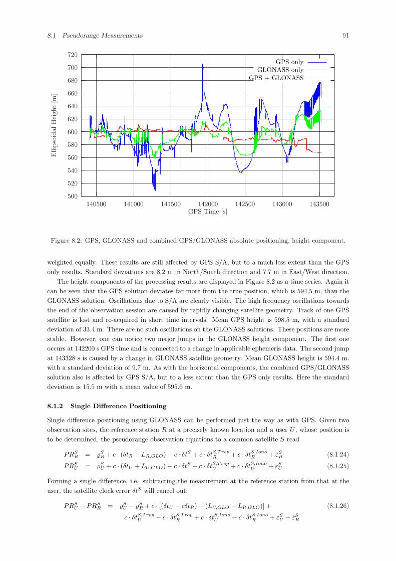
8.1 Pseudorange Measurements 91
500
520
540
560
580
600
620
640
660
680
700
720
140500 141000 141500 142000 142500 143000 143500
Elli
psoi
dalH
eigh
t[m
]
GPS Time [s]
GPS onlyGLONASS only
GPS + GLONASS
Figure 8.2: GPS, GLONASS and combined GPS/GLONASS absolute positioning, height component.
weighted equally. These results are still affected by GPS S/A, but to a much less extent than the GPSonly results. Standard deviations are 8.2 m in North/South direction and 7.7 m in East/West direction.
The height components of the processing results are displayed in Figure 8.2 as a time series. Again itcan be seen that the GPS solution deviates far more from the true position, which is 594.5 m, than theGLONASS solution. Oscillations due to S/A are clearly visible. The high frequency oscillations towardsthe end of the observation session are caused by rapidly changing satellite geometry. Track of one GPSsatellite is lost and re-acquired in short time intervals. Mean GPS height is 598.5 m, with a standarddeviation of 33.4 m. There are no such oscillations on the GLONASS solutions. These positions are morestable. However, one can notice two major jumps in the GLONASS height component. The first oneoccurs at 142200 s GPS time and is connected to a change in applicable ephemeris data. The second jumpat 143328 s is caused by a change in GLONASS satellite geometry. Mean GLONASS height is 594.4 m.with a standard deviation of 9.7 m. As with the horizontal components, the combined GPS/GLONASSsolution also is affected by GPS S/A, but to a less extent than the GPS only results. Here the standarddeviation is 15.5 m with a mean value of 595.6 m.
8.1.2 Single Difference Positioning
Single difference positioning using GLONASS can be performed just the way as with GPS. Given twoobservation sites, the reference station R at a precisely known location and a user U , whose position isto be determined, the pseudorange observation equations to a common satellite S read
PRSR = %S
R + c · (δtR + LR,GLO)− c · δtS + c · δtS,TropR + c · δtS,Iono
R + εSR (8.1.24)
PRSU = %S
U + c · (δtU + LU,GLO)− c · δtS + c · δtS,TropU + c · δtS,Iono
U + εSU (8.1.25)
Forming a single difference, i.e. subtracting the measurement at the reference station from that at theuser, the satellite clock error δtS will cancel out:
PRSU − PRS
R = %SU − %S
R + c · [(δtU − cδtR) + (LU,GLO − LR,GLO)] + (8.1.26)
c · δtS,TropU − c · δtS,Trop
R + c · δtS,IonoU − c · δtS,Iono
R + εSU − εS
R
92 8 OBSERVATIONS AND POSITION DETERMINATION
Supposed the user station is sufficiently close to the reference station, the path of the GLONASS satellitesignal through the ionosphere will be almost identical for reference station and user. Thus, the ionosphericdelay also will cancel out. This assumption holds true for distances of up to approximately 1000 km.
A similar assumption cannot be made for the tropospheric delay, because the troposphere immediatelysurrounds the receiver, and the signal travel path through the troposphere can be different even for nearbyreceivers, especially when the receivers are placed at different altitudes. This may be the case e.g. inmountainous regions or for aircraft approaching an airport. Thus, the tropospheric path delay does notcancel out in single difference positioning.
Denoting the single difference terms ∗U − ∗R as ∆∗UR, Eq. (8.1.26) therefore transforms to
∆PRSUR = ∆%S
UR + c · (∆δtUR + ∆LUR,GLO) + c ·∆δtS,TropUR + ∆εS
UR (8.1.27)
Linearizing the geometric range from user to satellite, we obtain
∆PRSUR = ∆%S
UR +x0 − xS
%S0
· (xR − x0) +y0 − yS
%S0
· (yR − y0) +z0 − zS
%S0
· (zR − z0) +
c · (∆δtUR,0 + ∆LUR,GLO,0) + (8.1.28)
c · [(∆δtUR + ∆LUR,GLO)− (∆δtUR,0 + ∆LUR,GLO,0)] + c ·∆δtS,TropUR + ∆εS
UR
where ∆%SUR now denotes %S
0 − %SR, the single difference geometric range from the approximate user
position to the satellite.Again shifting known and modeled terms to the left-hand side of the equation and considering a set of
observations to n GLONASS satellites, we obtain a system of observation equations in matrix notation:
~l = A · ~x + ~ε (8.1.29)
with
~l =
∆PR1UR −∆%1
UR − c · (∆δtUR,0 + ∆LUR,GLO,0)− c ·∆δt1,TropUR
∆PR2UR −∆%2
UR − c · (∆δtUR,0 + ∆LUR,GLO,0)− c ·∆δt2,TropUR
...∆PRn
UR −∆%nUR − c · (∆δtUR,0 + ∆LUR,GLO,0)− c ·∆δtn,Trop
UR
(8.1.30)
the vector of the known values,
A =
x0 − x1
%10
y0 − y1
%10
z0 − z1
%10
1
x0 − x2
%20
y0 − y2
%20
z0 − z2
%20
1
......
......
x0 − xn
%n0
y0 − yn
%n0
z0 − zn
%n0
1
(8.1.31)
the design matrix,
~x =
(xR − x0)(yR − y0)(zR − z0)
c · [(∆δtUR + ∆LUR,GLO)− (∆δtUR,0 + ∆LUR,GLO,0)]
(8.1.32)
the vector of the unknowns, and
~ε =
∆ε1UR
∆ε2UR...
∆εnUR
(8.1.33)
8.1 Pseudorange Measurements 93
the noise vector.In a combined GPS/GLONASS scenario, single differences from a user station U and a reference
station R to a GPS satellite i and a GLONASS satellite j can be formed analogously, starting from Eqs.(8.1.17) and (8.1.18), respectively:
PRiR = %i
R + c · (δtR + LR,GPS)− c · δti + c · δti,TropR + c · δti,Iono
R + εiR (8.1.34)
PRiU = %i
U + c · (δtU + LU,GPS)− c · δti + c · δti,TropU + c · δti,Iono
U + εiU (8.1.35)
PRjR = %j
R + c · (δtR + LR,GPS) + c · δtSys + c · δtR,HW − c · δtj + c · δtj,TropR + (8.1.36)
c · δtj,IonoR + εj
R
PRjU = %j
U + c · (δtU + LU,GPS) + c · δtSys + c · δtU,HW − c · δtj + c · δtj,TropU + (8.1.37)
c · δtj,IonoU + εj
U
yielding:
∆PRiUR = ∆%i
UR + c · (∆δtUR + ∆LUR,GPS) + c ·∆δti,TropUR + ∆εi
UR (8.1.38)
∆PRjUR = ∆%j
UR + c · (∆δtUR + ∆LUR,GPS) + c ·∆δtUR,HW + c ·∆δtj,TropUR + ∆εj
UR (8.1.39)
Besides the satellite clock errors and the ionospheric path delays, now also the time difference betweenGPS and GLONASS system time δtSys cancels out, however leaving the difference of the receiver inter-system hardware delays ∆δtUR,HW as a fifth unknown.
Again linearizing the geometric range from observer to satellite, shifting known and modeled termsto the left-hand sides of the equations and considering a set of m GPS and n GLONASS satellites, weobtain for the observation equation in matrix notation:
~l = A · ~x + ~ε (8.1.40)
with
~l =
∆PR1UR −∆%1
UR − c · (∆δtUR,0 + ∆LUR,GPS,0)− c ·∆δt1,TropUR
...
∆PRmUR −∆%m
UR − c · (∆δtUR,0 + ∆LUR,GPS,0)− c ·∆δtm,TropUR
∆PRm+1UR −∆%m+1
UR − c · (∆δtUR,0 + ∆LUR,GPS,0)− c ·∆δtUR,HW,0−c ·∆δtm+1,Trop
UR
...
∆PRm+nUR −∆%m+n
UR − c · (∆δtUR,0 + ∆LUR,GPS,0)− c ·∆δtUR,HW,0−c ·∆δtm+n,Trop
UR
(8.1.41)
the vector of the known values,
A =
x0 − x1
%10
y0 − y1
%10
z0 − z1
%10
1 0
......
......
...x0 − xm
%m0
y0 − ym
%m0
z0 − zm
%m0
1 0
x0 − xm+1
%m+10
y0 − ym+1
%m+10
z0 − zm+1
%m+10
1 1
......
......
...x0 − xm+n
%m+n0
y0 − ym+n
%m+n0
z0 − zm+n
%m+n0
1 1
(8.1.42)
94 8 OBSERVATIONS AND POSITION DETERMINATION
the design matrix,
~x =
(xR − x0)(yR − y0)(zR − z0)
c · [(∆δtUR + ∆LUR,GPS)− (∆δtUR,0 + ∆LUR,GPS,0)]c · (∆δtUR,HW −∆δtUR,HW,0)
(8.1.43)
the vector of the unknowns, and
~ε =
∆ε1UR...
∆εmUR
∆εm+1UR...
∆εm+nUR
(8.1.44)
the noise vector.An example of positioning results using GPS and GLONASS single difference positioning with pseu-
doranges is shown in Figure 8.3. Positions were computed from data logged by two 3S NavigationR-100/R-101 receivers, which were set up at known locations at the Institute of Geodesy and Navigation.Pseudorange and carrier phase measurements were logged every second for approximately one hour each,of which some forty minutes were common to both receivers. One of these receivers was used as referencestation, the other was treated as the user station. Its position was determined in this example. Observa-tion epochs at both receivers were not exactly synchronized. The data of the user station are the same asthe data already used for the absolute positioning example. The plot shows the deviation from the knownlocation of the antenna of the user station in the horizontal plane. GPS positions were computed fromcarrier smoothed L1 C/A-code pseudorange measurements. GLONASS positions were computed fromcarrier smoothed dual-frequency P-code measurements. Wherever possible, the ionospheric free linearcombination was formed. These observables used are not really identical for GPS and GLONASS, butwith P-code and dual-frequency measurements readily available on GLONASS, the best possible resultsfor each system are determined. GLONASS satellite positions were converted from PZ-90 to WGS84using the transformation according to (Roßbach et al., 1996).
The large deviations from the true position due to GPS S/A have been eliminated by the differencing ofobservations, but not completely. Due to the measurements at reference and user station not being exactlysynchronized, the effects of GPS S/A do not cancel entirely. This is most clearly visible in North/Southdirection, where the S/A effects on the absolute positioning also were most obvious. Standard deviationsof the computed positions from GPS only are 3.7 m in North/South direction and 1.3 m in East/Westdirection. Since there is no S/A on GLONASS, its effects cannot remain in the differenced positioningsolution due to imperfect synchronization of measurements. Consequently, positions computed only fromGLONASS range measurements scatter much less. Here the standard deviations are 1.4 m in North/Southdirection and 0.8 m in East/West direction. For the combined GPS/GLONASS positioning, all satellitemeasurements were weighted equally. These results are still affected by GPS S/A due to imperfectsynchronization, but to a much less extent than the GPS only results. Standard deviations are 1.6 m inNorth/South direction and 0.8 m in East/West direction.
The height components of the processing results are displayed in Figure 8.4 as a time series. Againit can be seen that the GPS solution deviates far more from the true position, which is 594.5 m, thanthe GLONASS solution. Oscillations due to S/A, caused by the imperfect synchronization, are clearlyvisible. Standard deviation of the GPS height component is 7.3 m around a mean value of 591.6 m.There are no such oscillations on the GLONASS solutions. These positions are more stable. However,one can notice one extended outlier around 142100 - 142200 s GPS time. The cause of this is not clear.
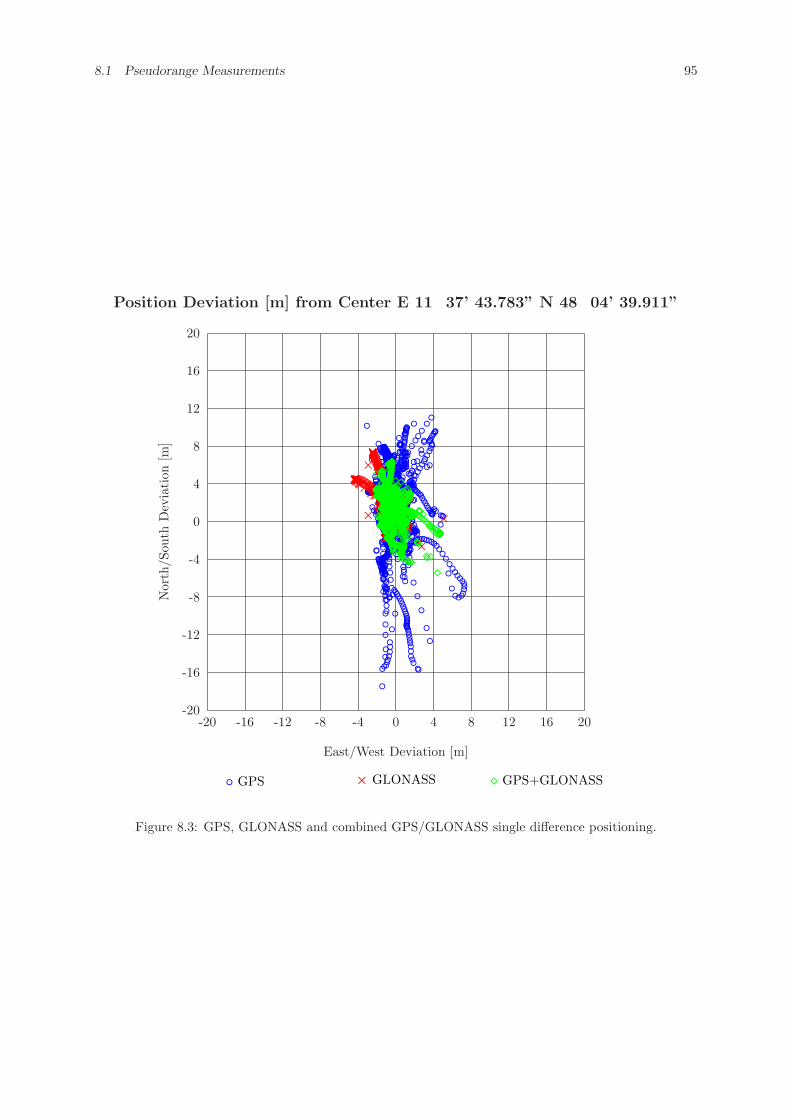
8.1 Pseudorange Measurements 95
Position Deviation [m] from Center E 11� 37’ 43.783” N 48� 04’ 39.911”
◦ GPS × GLONASS ¦ GPS+GLONASS
East/West Deviation [m]
-20 -16 -12 -8 -4 0 4 8 12 16 20
Nor
th/S
outh
Dev
iati
on[m
]
-20
-16
-12
-8
-4
0
4
8
12
16
20
◦◦◦◦
◦
◦◦◦◦◦◦◦◦◦◦◦◦◦◦
◦
◦
◦◦
◦
◦◦◦◦◦◦◦◦◦◦◦◦◦◦◦◦◦◦◦◦◦◦◦◦◦◦◦◦◦◦◦◦◦◦◦◦◦◦◦◦◦◦◦◦◦◦◦◦◦◦◦◦◦◦◦◦◦◦◦◦◦◦◦◦
◦◦◦◦◦◦◦◦◦◦◦◦◦◦◦◦◦◦◦◦◦◦◦◦◦◦◦◦◦◦◦◦◦◦◦◦◦◦◦◦◦◦
◦
◦◦◦◦◦◦◦◦◦◦◦◦◦◦◦◦◦
◦◦◦
◦◦◦◦◦◦◦◦◦◦◦◦◦◦◦◦◦◦◦◦◦◦◦◦◦◦◦◦◦◦◦◦◦◦◦◦◦◦◦◦◦◦◦◦
◦◦◦◦◦◦◦◦◦◦◦◦◦◦◦◦◦◦
◦◦◦◦◦◦
◦◦
◦◦◦
◦◦◦◦◦◦◦◦◦◦◦◦◦◦◦◦◦
◦◦◦◦◦◦◦◦
◦
◦◦◦◦◦◦◦◦◦◦
◦◦◦◦◦◦
◦◦◦◦◦◦◦◦◦◦◦◦◦◦◦
◦◦◦
◦◦◦◦◦◦◦◦◦◦◦◦◦◦◦◦◦◦◦◦◦◦◦◦◦◦◦◦◦◦◦◦◦◦◦◦◦◦◦◦◦◦◦◦◦◦◦◦◦◦◦◦◦◦◦◦◦◦◦◦◦◦◦◦◦◦◦◦◦◦◦◦◦◦◦◦
◦◦◦◦◦◦◦◦◦◦◦◦◦◦◦◦◦◦◦◦
◦◦
◦
◦◦◦
◦◦◦◦◦◦◦
◦◦◦◦◦◦◦◦◦◦◦
◦◦◦◦◦◦◦◦◦◦◦◦◦◦◦◦◦◦◦
◦◦◦◦◦◦◦◦◦◦◦◦◦◦◦◦◦◦◦
◦◦◦◦◦◦◦◦◦◦◦◦◦◦◦◦◦◦◦◦◦◦◦◦◦◦◦◦◦◦◦◦◦◦◦◦◦◦◦◦◦◦◦◦◦◦◦◦◦◦◦◦◦ ◦◦◦◦◦◦◦◦◦◦◦◦◦◦◦◦◦◦
◦◦◦
◦
◦
◦◦
◦◦◦◦
◦◦
◦◦◦◦◦◦
◦◦
◦◦◦◦◦◦◦◦◦◦◦◦◦◦◦◦◦◦
◦◦
◦◦◦◦◦◦◦◦
◦◦◦◦◦◦◦◦◦◦◦◦◦◦◦◦◦◦◦◦◦◦◦◦◦◦◦◦◦◦◦◦◦◦◦◦◦◦◦◦◦◦◦◦◦◦◦◦◦◦◦◦◦◦◦◦◦◦◦◦◦◦◦◦◦◦◦◦◦◦◦◦◦
◦◦◦◦◦◦◦◦◦
◦
◦◦◦◦◦◦◦
◦◦
◦◦◦◦
◦◦◦◦◦◦◦◦◦◦◦◦◦◦◦◦
◦◦◦◦◦◦
◦◦◦
◦◦
◦◦◦◦◦◦◦
◦◦◦◦◦◦◦◦◦◦◦◦◦◦◦◦◦◦◦◦
◦◦◦◦◦◦◦◦◦◦◦◦◦◦◦◦◦◦◦◦◦◦◦◦◦◦◦◦◦◦◦◦◦◦◦◦◦◦◦◦◦◦◦◦◦◦◦◦◦◦◦◦◦◦◦◦◦◦◦◦◦◦◦
◦
◦◦◦◦
◦◦◦◦
◦◦◦◦◦◦◦◦◦◦
◦◦◦◦◦◦◦◦◦◦◦
◦◦◦◦◦◦◦◦◦◦◦◦◦◦◦◦◦◦◦◦◦◦◦◦◦◦◦◦◦◦
◦◦◦◦◦◦◦◦◦◦◦◦
◦◦◦◦◦
◦◦
◦
◦◦
◦
◦◦◦◦◦◦◦◦◦◦◦◦◦◦◦◦◦◦◦◦◦◦◦◦◦◦◦◦◦◦◦◦◦◦◦◦◦◦◦◦◦◦◦◦◦◦◦◦◦◦◦◦◦◦◦◦◦◦◦◦◦◦◦◦◦◦◦◦◦◦◦◦◦◦◦◦◦◦◦◦◦◦◦◦◦◦◦◦◦◦◦◦◦◦◦◦◦◦◦◦◦◦◦◦◦◦◦◦◦◦◦◦◦◦◦◦◦◦◦◦◦◦
◦◦◦◦◦◦◦◦◦◦◦◦◦◦◦◦◦◦◦◦◦◦◦◦◦◦◦◦◦◦◦◦◦◦◦◦◦◦◦◦◦◦◦◦◦◦◦◦◦◦◦◦◦◦◦◦◦◦◦◦◦◦◦◦◦◦◦◦◦◦◦◦◦◦◦◦◦◦◦◦◦◦◦◦◦◦◦◦◦◦◦◦◦◦◦◦◦◦◦◦◦◦◦◦◦◦◦◦◦◦◦◦◦◦◦◦◦◦◦◦◦◦◦◦◦◦◦◦◦◦◦◦◦◦
◦◦◦◦◦◦◦◦◦◦◦◦◦◦◦◦
◦
◦
◦◦◦◦◦◦◦◦◦◦◦◦◦◦◦◦◦◦◦◦◦◦◦◦◦◦◦◦◦◦◦◦◦◦◦◦◦◦◦◦◦◦◦◦◦◦◦◦◦◦◦◦◦◦◦◦◦◦◦◦◦◦◦◦◦◦◦◦◦◦◦◦◦◦◦◦◦◦◦◦◦◦◦◦◦◦◦◦◦◦◦◦◦◦◦◦◦◦◦◦◦◦◦◦◦◦◦◦◦◦◦◦◦◦◦◦◦◦◦◦◦◦◦◦◦◦◦◦◦◦◦◦◦◦◦◦◦◦◦◦◦◦◦◦◦◦◦◦◦◦◦◦◦◦◦◦◦◦◦◦◦◦◦◦◦◦◦◦◦◦◦◦◦◦◦◦◦◦◦◦◦◦◦◦◦◦◦◦◦◦◦◦◦◦◦◦◦◦◦◦◦◦◦◦◦◦◦◦◦◦◦◦◦◦◦◦◦◦◦◦◦◦◦◦◦◦◦◦◦◦◦◦◦◦◦◦◦◦◦◦◦◦◦◦◦◦◦◦◦◦◦
◦◦◦◦◦◦◦◦◦◦◦◦◦◦◦◦◦◦◦◦◦◦◦◦◦◦◦◦◦◦◦◦◦◦◦◦◦◦◦◦◦◦◦◦◦◦◦◦◦◦◦◦◦◦◦◦◦◦◦◦◦◦◦◦◦
◦◦◦◦◦◦◦◦◦◦◦◦◦◦
◦◦◦◦◦◦◦◦◦◦◦◦◦◦◦◦◦◦◦
◦◦◦
◦◦◦
◦◦
◦◦◦◦◦◦◦
◦◦◦◦
◦◦
◦◦◦◦◦◦◦◦◦◦◦◦◦◦◦◦◦◦◦◦◦◦◦◦◦◦◦◦◦◦◦◦
◦◦◦◦◦◦◦◦◦◦◦◦◦◦◦◦◦◦◦◦◦◦◦◦◦◦◦◦◦◦◦◦◦◦◦◦◦◦◦◦◦◦◦◦◦◦◦◦◦◦◦◦◦◦
◦◦◦◦◦◦◦◦◦◦◦◦◦◦◦◦◦◦◦◦◦◦◦◦◦◦◦◦◦◦◦◦◦◦◦◦◦◦◦◦◦◦◦◦◦◦◦◦◦◦◦◦◦◦◦◦◦◦◦◦◦◦◦◦◦◦◦◦◦◦◦◦◦◦◦
◦◦◦◦◦◦◦◦◦◦◦◦◦◦◦◦◦◦◦◦◦◦◦◦◦◦◦◦◦◦◦◦◦◦◦◦◦◦◦◦◦◦◦◦◦◦◦◦◦◦◦◦◦◦◦◦◦◦◦◦◦◦◦◦◦◦◦◦◦◦◦◦◦◦◦◦◦◦
◦◦◦
◦◦◦◦◦
◦◦◦◦◦
◦
◦◦◦◦◦◦◦◦
◦◦◦◦◦◦◦◦
◦◦◦◦◦◦◦
◦◦◦◦◦◦◦◦◦◦◦◦◦◦◦◦◦◦◦◦◦◦◦◦◦◦◦◦◦◦◦◦◦◦◦◦◦
◦◦◦◦◦◦◦◦◦◦◦◦◦◦◦◦◦◦◦◦◦◦◦◦◦◦◦◦◦◦◦◦
◦◦◦◦◦◦◦◦◦◦◦◦◦◦◦◦◦◦◦◦◦◦◦◦◦◦◦◦◦◦◦◦◦◦◦◦◦◦◦◦◦◦◦◦◦
◦◦◦◦
◦◦◦◦◦◦◦◦◦◦◦◦◦◦
◦◦◦◦◦◦◦◦◦◦◦◦◦◦◦◦◦◦◦◦◦◦◦◦◦◦◦◦◦◦◦◦◦◦◦◦◦◦◦◦◦◦◦◦◦
◦◦◦◦◦◦◦◦◦◦◦◦◦◦◦◦◦◦◦◦◦◦◦◦◦◦◦◦◦◦◦◦◦◦◦◦◦◦◦◦◦◦◦◦◦◦◦◦◦◦◦◦◦◦◦◦◦◦◦◦◦◦◦◦◦◦◦◦◦◦◦◦◦◦◦◦◦◦◦◦◦◦◦◦◦◦◦◦◦◦◦◦◦◦◦◦◦◦◦◦◦◦◦◦◦◦◦◦◦◦◦◦◦◦◦◦◦◦◦◦◦◦◦◦◦◦◦◦◦◦◦◦◦◦◦◦◦◦◦◦◦◦◦◦◦◦◦◦◦◦◦◦◦◦◦◦◦◦◦◦◦◦◦◦◦◦◦◦◦◦◦◦◦◦◦◦◦◦◦◦◦◦◦◦◦◦◦◦◦◦◦◦◦◦◦◦◦◦◦◦◦◦◦◦◦◦◦◦◦◦◦◦◦◦◦◦◦◦◦◦◦◦◦
◦◦◦◦◦◦◦◦◦◦◦◦◦◦◦◦◦◦◦◦◦◦◦◦◦◦◦◦◦◦◦◦◦◦◦◦◦◦◦◦◦◦◦◦◦◦◦◦◦◦◦◦◦◦◦◦◦◦◦◦◦◦◦◦◦◦×××××××××××××××××××××××××××××××××××××××××××××××××××××××××××××××××××××××××××××××××××××××××××××××××××××××××××××××××××××××××××××××××××××××××××××××××××××××××××××××××××××××××××××××××××××××××××××××××××××××××××××××××××××××××××××××××××××××××××××××××××××××××××××××××××××××××××××××××××××××××××××××××××××××××××××××××××××××××××××××××××××××
×××××××××
××
×××××××××××××××××××××××××××××××××××××××××××××××××××××××××××××××××××××××××××××××××××××××××××××××××××××××××××××××××××××××××××××××××××××××××××××××××××××××××××××××××××××××××××××××××××××××××××××××××××××××××××××××××××××××××××××××××××××××××××××××××××××××××××××××××××××××××××××××××××××××××××××××××××××××××××××××××××××××××××××××××××××××××××××××××××××××××××××××××××××××××××××××××××××××××××××××××××××××××××××××××××××××××××××××××××××××××××××××××××××××××××××××××××××××××××××××××××××××××××××××××××××××××××××××××××××××××××××××××××××××××××××××××××××
××××××××
×
××××××××
××××××××××××××××××××××××××××××××××××××××××××××××××××××××××××××××××××××××××××××××××××××××××××××××××××××××××××××××××××
×××××××××××××××××××××××××××××××××××××××××××××××××××××××××××××××××××××××××××××××××××××××××××××××××××××××××××××××××××××××××××××××××××××××××××××××××××××××××××××××××××××××××××××××××××××××××××××××××××××××××××××××××××××××××××××××××××××××××××××××××××××××××××××××××××××××××××××××××××××××××××××××××××××××××××××××××××××××××××××××××××××××××××××××××××××××××××××××××××××××××××××××××××××××××××××××××××××××××××××××××××××××××××××××××××××××××××××××× ××××××××××××××××××××××××××××××××××××××××××××××××××××××××××××××××××××××××××××××××××××××××××××××××××××××××××××××××××××××××××××××××××××××××××××××××××××××××××××××××××××××××××××××××××××××××××××××××××××××××××××××××××××××××××××××××××××××××××××××××××××××××××××××××××××××××××××××××××××××××××××××
×
×××××××××××××××××××××××××××××××××××××××××××××
××××××××××××××××××××××××××××××××××××××××××××××××××××××××××××××××××××××××××××××××××××××××××××××××××××××××××××××
×××××××××××××××××××××××××××××××××××××
×××××××××××××××××××××××××××××××××××××××××××××××××××××××××××××××××××××××××××××××××××××××××××××××××××××
××××××××××××××××××××××××××××××××××××××××××××××××××××××××××××××××××××××××××××××××××××××××××××××××××××××××××××××××××××××××××××××××××××××××××××××××××
¦ ¦¦¦¦ ¦¦ ¦¦¦¦¦¦¦¦¦¦¦¦¦¦
¦¦¦¦¦¦¦¦¦¦¦¦¦¦¦¦¦¦¦¦¦¦¦¦¦¦¦¦¦¦¦¦¦¦¦¦¦¦¦¦¦¦¦¦¦¦¦¦¦¦¦¦¦¦¦¦¦¦¦¦¦¦¦¦¦¦¦¦¦¦¦¦¦¦¦¦¦¦¦¦¦¦¦¦¦¦¦¦¦¦¦¦¦¦¦¦¦¦¦¦¦¦¦¦¦¦¦¦¦¦¦¦¦¦¦¦¦¦¦¦¦
¦¦¦¦¦¦¦¦¦¦¦¦¦¦¦¦¦¦¦¦¦¦¦¦¦¦¦¦¦¦¦¦¦¦¦¦¦¦¦¦¦¦¦¦¦¦¦¦¦¦¦¦¦¦¦¦¦¦¦¦¦¦¦¦¦¦¦¦¦¦¦¦¦¦¦¦¦¦¦¦¦¦¦¦¦¦¦¦¦¦ ¦¦¦¦ ¦¦¦¦¦¦¦¦¦¦¦¦¦¦¦¦¦¦¦¦
¦¦¦¦¦¦ ¦¦¦¦¦¦¦¦¦¦¦¦¦¦¦¦¦¦¦¦¦¦¦¦¦¦¦¦¦¦¦¦¦¦¦¦
¦¦¦¦¦¦¦¦¦¦¦¦¦¦¦¦¦¦¦¦¦¦¦¦¦¦¦¦¦¦¦¦¦¦¦¦¦¦¦¦¦¦¦¦¦¦¦¦¦¦¦¦¦¦¦¦¦¦¦¦¦¦¦¦¦¦¦¦¦¦¦¦¦¦¦¦¦¦¦¦¦¦¦¦¦¦¦¦¦¦¦¦¦¦¦¦¦¦¦¦¦¦
¦¦¦¦¦¦¦¦¦¦¦¦¦¦¦¦¦¦¦¦¦¦¦¦¦¦¦¦¦¦¦¦¦¦¦¦¦¦¦¦¦¦¦¦¦¦¦¦¦¦¦¦¦¦¦¦¦¦¦¦¦¦¦¦¦¦¦¦¦¦¦¦¦¦¦¦¦¦¦¦¦¦¦¦¦¦¦¦¦¦¦¦¦¦¦¦¦¦¦¦¦¦¦¦¦¦¦¦¦¦¦¦¦¦¦¦¦¦¦¦¦¦¦¦¦¦¦¦¦¦¦¦¦
¦¦¦ ¦¦¦¦
¦¦ ¦¦¦¦¦¦¦¦¦¦¦¦¦¦¦¦¦¦¦¦¦¦¦¦¦¦¦¦¦¦¦¦¦¦¦¦¦¦¦¦¦
¦¦¦¦¦¦¦¦¦¦¦¦¦¦¦¦¦¦¦¦¦¦¦¦¦¦¦¦¦¦¦¦¦¦¦¦¦¦¦¦¦¦¦¦¦¦¦¦¦¦¦¦¦¦¦¦¦¦¦¦¦¦¦¦¦¦¦¦
¦¦¦¦¦¦¦¦¦¦ ¦¦¦¦¦¦¦¦¦¦¦¦¦¦¦¦¦¦¦¦¦¦¦¦¦¦¦¦¦¦¦¦¦¦¦¦¦¦ ¦¦¦¦¦¦¦¦¦ ¦¦¦¦¦¦¦¦¦¦¦¦¦¦¦¦¦¦¦¦¦¦¦¦¦¦¦¦¦¦¦¦¦¦¦¦¦¦¦¦¦¦¦¦¦¦¦¦¦¦¦¦¦¦¦¦¦¦¦¦¦¦¦¦¦¦¦¦¦¦¦¦¦¦¦¦¦¦¦¦¦¦¦¦¦¦¦¦¦
¦¦¦¦¦¦¦¦¦¦¦¦¦¦¦¦
¦¦¦¦¦¦¦¦¦¦¦¦¦¦¦¦¦¦¦¦¦¦¦¦¦¦¦¦¦¦¦¦¦¦¦¦¦¦¦
¦¦¦¦¦¦¦¦¦¦¦¦¦¦¦¦¦¦¦¦
¦¦¦
¦¦¦¦¦¦¦¦¦¦¦¦¦¦¦¦¦¦¦¦¦¦¦¦¦¦¦¦¦¦¦¦¦¦¦¦¦¦¦¦¦¦¦¦¦¦¦¦¦¦¦¦¦¦¦¦¦¦¦¦¦¦¦¦¦¦¦¦¦¦¦¦¦¦¦¦¦¦¦¦¦¦¦¦¦
¦¦¦¦¦¦¦¦¦¦¦¦¦¦¦¦¦¦¦¦¦¦¦¦¦¦¦¦¦¦¦¦¦¦¦¦¦¦¦¦¦¦¦¦¦¦¦¦¦¦¦¦¦¦¦¦¦¦¦¦¦¦¦¦¦¦¦¦¦¦¦¦¦¦¦¦¦¦¦¦¦¦¦¦¦¦¦¦¦¦¦¦¦¦¦¦¦¦¦¦¦¦¦¦¦¦¦¦¦¦¦¦¦¦¦¦¦¦¦¦¦¦¦¦¦¦¦¦¦¦¦¦¦¦¦¦¦¦¦¦¦¦¦¦¦¦¦¦¦¦¦¦¦¦¦¦¦¦¦¦¦¦¦¦¦¦¦¦¦¦¦¦¦¦¦¦¦¦¦¦¦¦¦¦¦¦¦¦¦¦¦¦¦¦¦¦¦¦¦¦¦¦¦¦¦¦¦¦¦¦¦¦¦¦¦¦¦¦¦¦¦¦¦¦¦¦¦¦¦¦¦¦¦¦¦¦¦¦¦¦¦¦¦¦¦¦¦¦¦¦¦¦¦¦¦¦¦¦¦¦¦¦¦¦¦¦¦¦¦¦¦¦¦¦¦¦¦¦¦¦¦¦¦¦¦¦¦¦¦¦¦¦¦¦¦¦¦¦¦¦¦¦¦¦¦¦¦¦¦¦¦¦¦¦¦¦¦¦¦¦¦¦¦¦¦¦¦¦¦¦¦¦¦¦¦¦¦¦¦¦¦¦¦¦¦¦¦¦¦¦¦¦¦¦¦¦¦¦¦¦¦¦¦¦¦¦¦¦¦¦¦¦¦¦¦¦¦¦¦¦¦¦¦¦¦¦¦¦¦¦¦¦¦¦¦¦¦¦¦¦¦¦¦¦¦¦¦¦¦¦¦¦¦¦¦¦¦¦¦¦¦¦¦¦¦¦¦¦¦¦¦¦¦¦¦¦¦¦¦¦¦¦¦¦¦¦¦¦¦¦¦¦¦¦¦¦¦¦¦¦¦¦¦¦¦¦¦¦¦¦¦¦¦¦¦¦¦¦¦¦¦¦¦¦¦¦¦¦¦¦¦¦¦¦¦¦¦¦¦¦¦¦¦¦¦¦¦¦¦¦¦¦¦¦¦¦¦¦¦¦¦¦¦¦¦¦¦¦¦¦¦¦¦¦¦¦¦¦¦
¦
¦
¦ ¦¦¦¦¦¦¦¦¦¦¦¦¦¦¦¦¦¦¦
¦¦¦
¦¦¦
¦¦¦¦ ¦¦¦¦¦¦¦¦¦¦¦¦¦¦¦¦¦¦¦¦¦¦¦¦¦¦¦¦¦¦
¦¦¦¦¦¦¦¦¦¦¦¦¦¦¦¦¦¦¦¦¦¦¦¦¦¦¦¦¦¦¦¦¦¦¦¦¦¦¦¦¦¦¦¦¦¦¦¦¦¦¦¦¦¦¦¦¦¦¦¦¦¦¦¦¦¦¦¦¦¦¦¦¦¦¦¦¦¦¦¦¦¦¦¦¦¦¦¦¦¦¦¦¦¦¦¦¦¦¦¦¦¦¦¦¦¦¦¦¦¦¦¦¦¦¦¦¦¦¦¦¦¦¦¦¦
¦¦¦¦¦¦¦¦¦¦¦¦¦¦¦¦¦¦¦¦¦¦¦¦¦¦¦¦¦¦¦¦¦¦¦¦¦¦¦¦¦¦¦¦¦¦¦¦¦¦¦¦¦¦¦¦¦¦¦¦¦¦¦¦¦¦¦¦¦¦¦¦¦¦¦¦¦¦¦¦¦¦
¦¦¦¦¦
¦¦¦¦¦
¦
¦¦¦¦¦¦¦¦¦
¦¦¦¦¦¦¦¦¦¦¦¦¦¦¦¦¦¦¦¦¦¦¦¦¦
¦¦¦¦¦¦¦¦¦¦¦¦¦¦¦¦¦¦¦¦¦¦¦¦¦¦¦¦¦¦¦¦¦¦¦¦¦¦¦¦¦¦¦¦¦¦¦¦¦¦¦¦¦¦¦¦¦¦¦
¦¦¦¦¦¦¦¦¦¦¦¦¦¦¦¦¦¦¦¦¦¦¦¦¦¦¦¦¦¦¦¦¦¦¦¦¦¦¦¦¦¦¦¦¦¦¦¦¦¦
¦
¦
¦¦
¦
¦
¦¦¦¦¦¦¦¦¦¦
¦¦¦¦¦¦¦¦¦¦¦¦¦¦¦¦¦¦¦¦¦¦¦¦¦¦¦¦¦¦¦¦¦¦¦¦¦¦¦¦¦¦¦¦¦¦¦¦¦¦¦¦¦¦¦¦¦¦¦¦¦¦¦¦¦¦¦¦¦¦¦¦¦¦¦¦¦¦¦¦¦¦¦¦¦¦¦¦¦
¦¦¦¦¦¦¦¦¦¦¦¦¦¦¦¦¦¦¦¦¦¦¦¦¦¦¦¦¦¦¦¦¦¦¦¦¦¦¦¦¦¦¦¦¦¦¦¦¦¦¦¦¦¦¦¦¦¦¦¦¦¦¦¦¦¦¦¦¦¦¦¦¦¦¦¦¦¦¦¦¦¦¦¦¦¦¦¦¦¦¦¦¦¦¦¦¦¦¦¦¦¦¦¦¦¦¦¦¦¦¦¦¦¦¦¦¦¦¦¦¦¦¦¦¦¦¦¦¦¦¦¦¦¦¦¦¦¦¦¦¦¦¦¦¦¦¦¦¦¦¦¦¦¦¦¦¦¦¦¦¦¦¦¦¦¦¦¦¦¦¦¦¦¦¦¦¦¦¦¦¦¦¦¦¦¦¦¦¦¦¦¦¦¦¦¦¦¦¦¦¦¦¦¦¦¦¦¦¦¦¦¦¦¦¦¦¦¦¦¦¦¦¦¦¦¦¦¦¦¦¦¦¦¦¦¦¦¦¦¦¦¦¦¦¦¦¦
Figure 8.3: GPS, GLONASS and combined GPS/GLONASS single difference positioning.
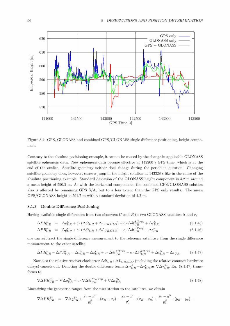
96 8 OBSERVATIONS AND POSITION DETERMINATION
570
580
590
600
610
620
141000 141500 142000 142500 143000 143500
Elli
psoi
dalH
eigh
t[m
]
GPS Time [s]
GPS onlyGLONASS only
GPS + GLONASS
Figure 8.4: GPS, GLONASS and combined GPS/GLONASS single difference positioning, height compo-nent.
Contrary to the absolute positioning example, it cannot be caused by the change in applicable GLONASSsatellite ephemeris data. New ephemeris data become effective at 142200 s GPS time, which is at theend of the outlier. Satellite geometry neither does change during the period in question. Changingsatellite geometry does, however, cause a jump in the height solution at 143328 s like in the cause of theabsolute positioning example. Standard deviation of the GLONASS height component is 4.2 m arounda mean height of 590.5 m. As with the horizontal components, the combined GPS/GLONASS solutionalso is affected by remaining GPS S/A, but to a less extent than the GPS only results. The meanGPS/GLONASS height is 591.7 m with a standard deviation of 4.2 m.
8.1.3 Double Difference Positioning
Having available single differences from two observers U and R to two GLONASS satellites S and r,
∆PRSUR = ∆%S
UR + c · (∆δtUR + ∆LUR,GLO) + c ·∆δtS,TropUR + ∆εS
UR (8.1.45)
∆PRrUR = ∆%r
UR + c · (∆δtUR + ∆LUR,GLO) + c ·∆δtr,TropUR + ∆εr
UR (8.1.46)
one can subtract the single difference measurement to the reference satellite r from the single differencemeasurement to the other satellite:
∆PRSUR −∆PRr
UR = ∆%SUR −∆%r
UR + c ·∆δtS,TropUR − c ·∆δtr,Trop
UR + ∆εSUR −∆εr
UR (8.1.47)
Now also the relative receiver clock error ∆δtUR+∆LUR,GLO (including the relative common hardwaredelays) cancels out. Denoting the double difference terms ∆ ∗S
UR −∆∗rUR as ∇∆∗Sr
UR, Eq. (8.1.47) trans-forms to
∇∆PRSrUR = ∇∆%Sr
UR + c · ∇∆δtSr,TropUR +∇∆εSr
UR (8.1.48)
Linearizing the geometric ranges from the user station to the satellites, we obtain
∇∆PRSrUR = ∇∆%Sr
UR +x0 − xS
%S0
· (xR − x0)− x0 − xr
%r0
· (xR − x0) +y0 − yS
%S0
· (yR − y0)−
8.1 Pseudorange Measurements 97
y0 − yr
%r0
· (yR − y0) +z0 − zS
%S0
· (zR − z0)− z0 − zr
%r0
· (zR − z0) + (8.1.49)
c · ∇∆δtSr,TropUR +∇∆εSr
UR
where ∇∆%SrUR now denotes (%S
0 − %SR) − (%r
0 − %rR), the double difference geometric range from the
approximate user position to the satellites.Again shifting known and modeled terms to the left-hand side of the equation and considering a set
of observations to n GLONASS satellites (not including the reference satellite r), we obtain a system ofobservation equations in matrix notation:
~l = A · ~x + ~ε (8.1.50)
with
~l =
∇∆PR1rUR −∇∆%1r
UR − c · ∇∆δt1r,TropUR
∇∆PR2rUR −∇∆%2r
UR − c · ∇∆δt2r,TropUR
...∇∆PRnr
UR −∇∆%nrUR − c · ∇∆δtnr,Trop
UR
(8.1.51)
the vector of the known values,
A =
x0 − x1
%10
− x0 − xr
%r0
y0 − y1
%10
− y0 − yr
%r0
z0 − z1
%10
− z0 − zr
%r0
x0 − x2
%20
− x0 − xr
%r0
y0 − y2
%20
− y0 − yr
%r0
z0 − z2
%20
− z0 − zr
%r0
......
...x0 − xn
%n0
− x0 − xr
%r0
y0 − yn
%n0
− y0 − yr
%r0
z0 − zn
%n0
− z0 − zr
%r0
(8.1.52)
the design matrix,
~x =
(xR − x0)(yR − y0)(zR − z0)
(8.1.53)
the vector of the unknowns, and
~ε =
∇∆ε1rUR
∇∆ε2rUR
...∇∆εnr
UR
(8.1.54)
the noise vector.In a combined GPS/GLONASS scenario, with a GPS satellite i, a GLONASS satellite j and the
reference satellite r, two cases must be distinguished, depending on whether the reference satellite is aGPS or a GLONASS satellite:
1. The reference satellite is a GPS satellite.
From the single difference observations
∆PRiUR = ∆%i
UR + c · (∆δtUR + ∆LUR,GPS) + c ·∆δti,TropUR + ∆εi
UR (8.1.55)
∆PRjUR = ∆%j
UR + c · (∆δtUR + ∆LUR,GPS) + c ·∆δtUR,HW + (8.1.56)
c ·∆δtj,TropUR + ∆εj
UR
∆PRrUR = ∆%r
UR + c · (∆δtUR + ∆LUR,GPS) + c ·∆δtr,TropUR + ∆εr
UR (8.1.57)
98 8 OBSERVATIONS AND POSITION DETERMINATION
one can form the double differences
∇∆PRirUR = ∇∆%ir
UR + c · ∇∆δtir,TropUR +∇∆εir
UR (8.1.58)
∇∆PRjrUR = ∇∆%jr
UR + c ·∆δtUR,HW + c · ∇∆δtjr,TropUR +∇∆εjr
UR (8.1.59)
The single difference receiver inter-system hardware delay ∆δtUR,HW remains in the mixed GLO-NASS/GPS double difference.
2. The reference satellite is a GLONASS satellite.
From the single difference observations
∆PRiUR = ∆%i
UR + c · (∆δtUR + ∆LUR,GPS) + c ·∆δti,TropUR + ∆εi
UR (8.1.60)
∆PRjUR = ∆%j
UR + c · (∆δtUR + ∆LUR,GPS) + c ·∆δtUR,HW + (8.1.61)
c ·∆δtj,TropUR + ∆εj
UR
∆PRrUR = ∆%r
UR + c · (∆δtUR + ∆LUR,GPS) + c ·∆δtUR,HW + (8.1.62)
c ·∆δtr,TropUR + ∆εr
UR
one can form the double differences
∇∆PRirUR = ∇∆%ir
UR − c ·∆δtUR,HW + c · ∇∆δtir,TropUR +∇∆εir
UR (8.1.63)
∇∆PRjrUR = ∇∆%jr
UR + c · ∇∆δtjr,TropUR +∇∆εjr
UR (8.1.64)
The single difference receiver inter-system hardware delay ∆δtUR,HW now cancels out in the GLO-NASS/GLONASS double difference, but it shows up in the mixed GPS/GLONASS double differencewith the opposite sign instead.
The single difference receiver inter-system hardware delay ∆δtUR,HW remains as a fourth unknownin the double difference observation equations. Depending on whether the reference satellite is a GPS ora GLONASS satellite, it shows up with opposite sign either at the GLONASS or the GPS satellites.
Considering this fact, we obtain for the observation equations of a set of m GPS and n GLONASSsatellites (not including the reference satellite r):
~l = A · ~x + ~ε (8.1.65)
with
~l =
∇∆PR1rUR −∇∆%1r
UR − kGPS · c ·∆δtUR,HW,0 − c · ∇∆δt1r,TropUR
...∇∆PRmr
UR −∇∆%mrUR − kGPS · c ·∆δtUR,HW,0 − c · ∇∆δtmr,Trop
UR
∇∆PRm+1,rUR −∇∆%m+1,r
UR − kGLONASS · c ·∆δtUR,HW,0 − c · ∇∆δtm+1,r,TropUR
...∇∆PRm+n,r
UR −∇∆%m+n,rUR − kGLONASS · c ·∆δtUR,HW,0 − c · ∇∆δtm+n,r,Trop
UR
(8.1.66)
with
kGPS =
{0 , r ∈ GPS
−1 , r ∈ GLONASS
kGLONASS =
{1 , r ∈ GPS0 , r ∈ GLONASS
8.1 Pseudorange Measurements 99
the vector of the known values,
A=
x0 − x1
%10
− x0 − xr
%r0
y0 − y1
%10
− y0 − yr
%r0
z0 − z1
%10
− z0 − zr
%r0
kGPS
......
......
x0 − xm
%m0
− x0 − xr
%r0
y0 − ym
%m0
− y0 − yr
%r0
z0 − zm
%m0
− z0 − zr
%r0
kGPS
x0 − xm+1
%m+10
− x0 − xr
%r0
y0 − ym+1
%m+10
− y0 − yr
%r0
z0 − zm+1
%m+10
− z0 − zr
%r0
kGLONASS
......
......
x0 − xm+n
%m+n0
− x0 − xr
%r0
y0 − ym+n
%m+n0
− y0 − yr
%r0
z0 − zm+n
%m+n0
− z0 − zr
%r0
kGLONASS
(8.1.67)
the design matrix,
~x =
(xR − x0)(yR − y0)(zR − z0)
c · (∆δtUR,HW −∆δtUR,HW,0)
(8.1.68)
the vector of the unknowns, and
~ε =
∇∆ε1rUR
...∇∆εmr
UR
∇∆εm+1,rUR...
∇∆εm+n,rUR
(8.1.69)
the noise vector.
The single difference receiver inter-system hardware delay ∆δtUR,HW will, however, cancel, if twoseparate reference satellites for GPS and for GLONASS are chosen. In that case, from the single differenceobservations
∆PRiUR = ∆%i
UR + c · (∆δtUR+∆LUR,GPS) + c ·∆δti,TropUR + ∆εi
UR (8.1.70)
∆PRrGP S
UR = ∆%rGP S
UR + c · (∆δtUR+∆LUR,GPS) + c ·∆δtrGP S ,Trop
UR + ∆εrGP S
UR (8.1.71)
∆PRjUR = ∆%j
UR + c · (∆δtUR+∆LUR,GPS) + c ·∆δtUR,HW + c ·∆δtj,TropUR + ∆εj
UR (8.1.72)
∆PRrGLO
UR = ∆%rGLO
UR + c · (∆δtUR+∆LUR,GPS) + c ·∆δtUR,HW + c ·∆δtrGP S ,Trop
UR + (8.1.73)
∆εrGP S
UR
to GPS satellites i and rGPS and GLONASS satellites j and rGLO the double difference observations
∇∆PRirGP S
UR = ∇∆%irGP S
UR + c · ∇∆δtirGP S ,Trop
UR +∇∆εirGP S
UR (8.1.74)
∇∆PRjrGLO
UR = ∇∆%jrGLO
UR + c · ∇∆δtjrGLO,TropUR +∇∆εjrGLO
UR (8.1.75)
can be formed.
Again shifting all known and modeled terms to the left-hand side of the equation and considering a setof observations to m GPS and n GLONASS satellites (not including the respective reference satellites),we obtain a system of observation equations in matrix notation:
~l = A · ~x + ~ε (8.1.76)
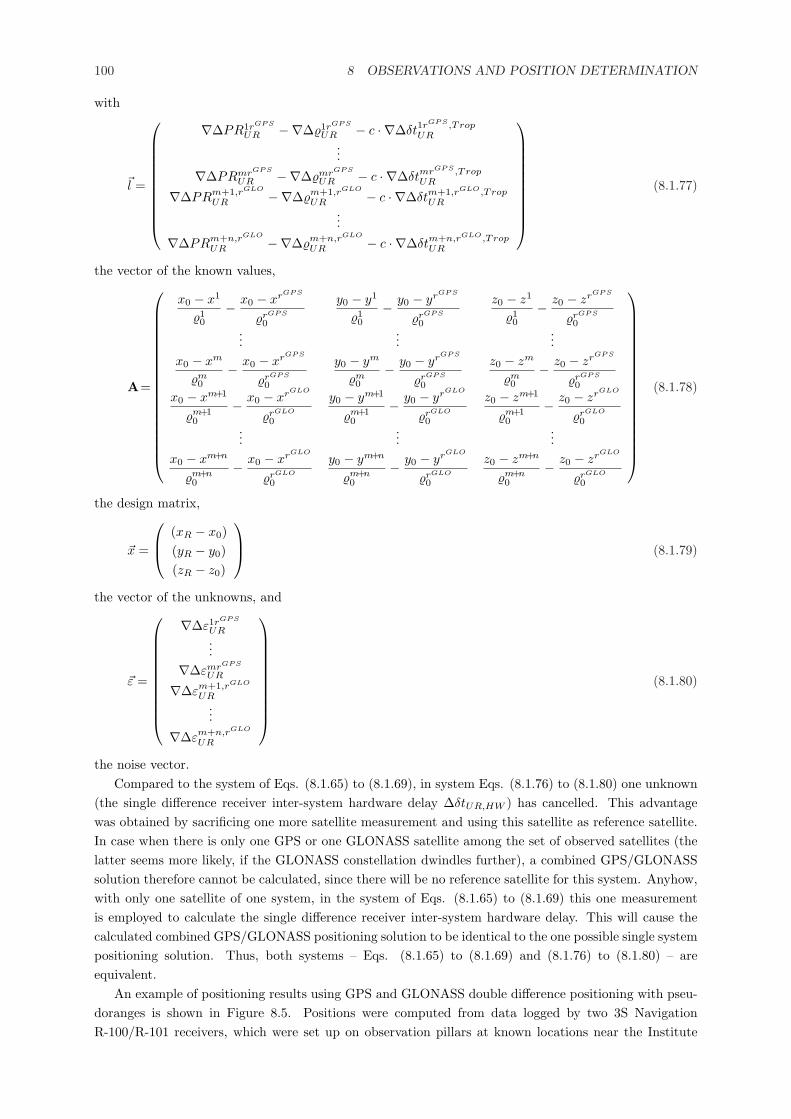
100 8 OBSERVATIONS AND POSITION DETERMINATION
with
~l =
∇∆PR1rGP S
UR −∇∆%1rGP S
UR − c · ∇∆δt1rGP S ,TropUR
...
∇∆PRmrGP S
UR −∇∆%mrGP S
UR − c · ∇∆δtmrGP S ,TropUR
∇∆PRm+1,rGLO
UR −∇∆%m+1,rGLO
UR − c · ∇∆δtm+1,rGLO,TropUR
...
∇∆PRm+n,rGLO
UR −∇∆%m+n,rGLO
UR − c · ∇∆δtm+n,rGLO,TropUR
(8.1.77)
the vector of the known values,
A=
x0 − x1
%10
− x0 − xrGP S
%rGP S
0
y0 − y1
%10
− y0 − yrGP S
%rGP S
0
z0 − z1
%10
− z0 − zrGP S
%rGP S
0...
......
x0 − xm
%m0
− x0 − xrGP S
%rGP S
0
y0 − ym
%m0
− y0 − yrGP S
%rGP S
0
z0 − zm
%m0
− z0 − zrGP S
%rGP S
0
x0 − xm+1
%m+10
− x0 − xrGLO
%rGLO
0
y0 − ym+1
%m+10
− y0 − yrGLO
%rGLO
0
z0 − zm+1
%m+10
− z0 − zrGLO
%rGLO
0...
......
x0 − xm+n
%m+n0
− x0 − xrGLO
%rGLO
0
y0 − ym+n
%m+n0
− y0 − yrGLO
%rGLO
0
z0 − zm+n
%m+n0
− z0 − zrGLO
%rGLO
0
(8.1.78)
the design matrix,
~x =
(xR − x0)(yR − y0)(zR − z0)
(8.1.79)
the vector of the unknowns, and
~ε =
∇∆ε1rGP S
UR...
∇∆εmrGP S
UR
∇∆εm+1,rGLO
UR...
∇∆εm+n,rGLO
UR
(8.1.80)
the noise vector.Compared to the system of Eqs. (8.1.65) to (8.1.69), in system Eqs. (8.1.76) to (8.1.80) one unknown
(the single difference receiver inter-system hardware delay ∆δtUR,HW ) has cancelled. This advantagewas obtained by sacrificing one more satellite measurement and using this satellite as reference satellite.In case when there is only one GPS or one GLONASS satellite among the set of observed satellites (thelatter seems more likely, if the GLONASS constellation dwindles further), a combined GPS/GLONASSsolution therefore cannot be calculated, since there will be no reference satellite for this system. Anyhow,with only one satellite of one system, in the system of Eqs. (8.1.65) to (8.1.69) this one measurementis employed to calculate the single difference receiver inter-system hardware delay. This will cause thecalculated combined GPS/GLONASS positioning solution to be identical to the one possible single systempositioning solution. Thus, both systems – Eqs. (8.1.65) to (8.1.69) and (8.1.76) to (8.1.80) – areequivalent.
An example of positioning results using GPS and GLONASS double difference positioning with pseu-doranges is shown in Figure 8.5. Positions were computed from data logged by two 3S NavigationR-100/R-101 receivers, which were set up on observation pillars at known locations near the Institute
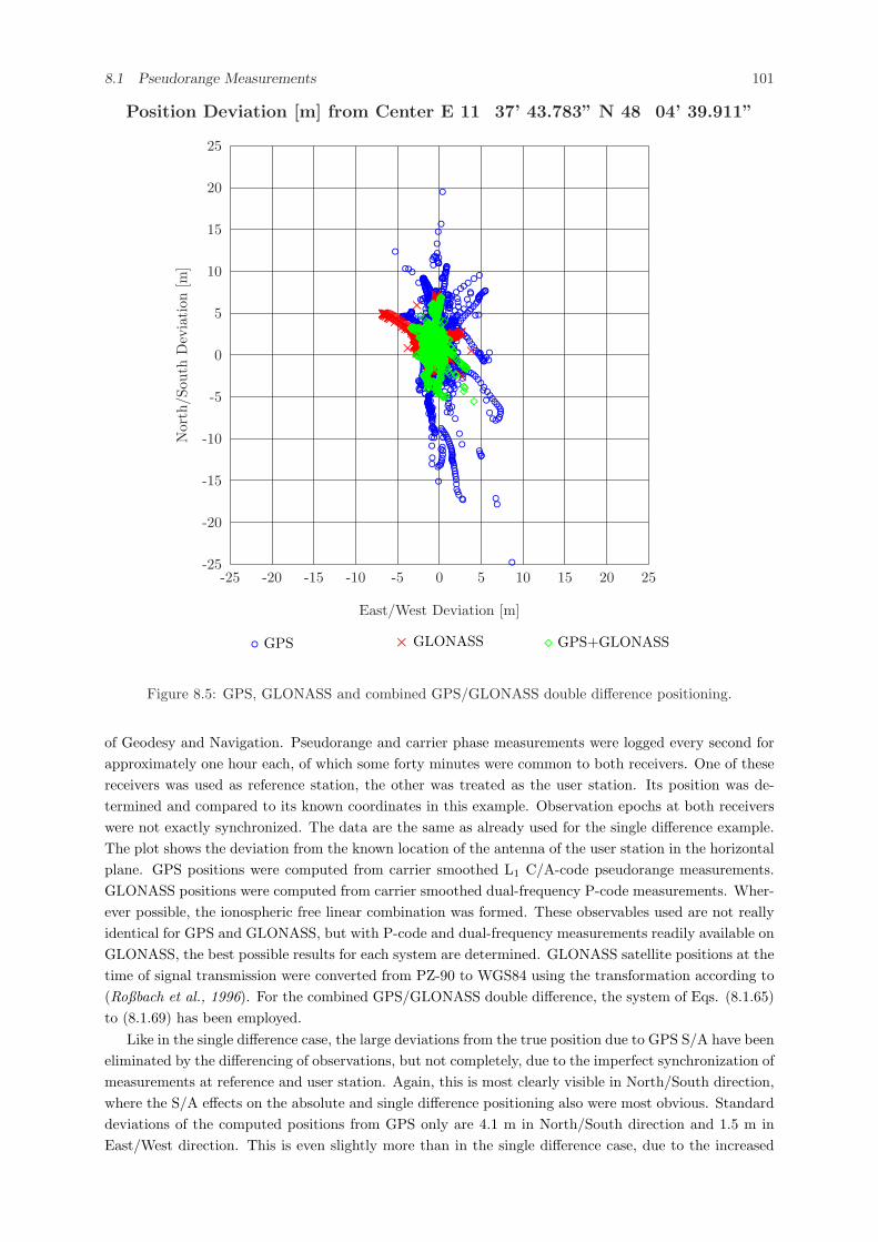
8.1 Pseudorange Measurements 101
Position Deviation [m] from Center E 11� 37’ 43.783” N 48� 04’ 39.911”
◦ GPS × GLONASS ¦ GPS+GLONASS
East/West Deviation [m]
-25 -20 -15 -10 -5 0 5 10 15 20 25
Nor
th/S
outh
Dev
iati
on[m
]
-25
-20
-15
-10
-5
0
5
10
15
20
25
◦
◦
◦◦◦
◦
◦
◦◦◦◦◦◦◦◦◦◦◦◦◦
◦
◦
◦◦
◦
◦◦◦◦◦◦◦◦ ◦◦◦◦◦ ◦◦◦◦◦◦◦◦◦◦◦◦◦◦◦◦◦◦◦◦◦◦◦◦◦◦◦◦◦◦◦◦◦◦◦ ◦◦◦◦◦◦◦◦◦◦◦◦◦◦◦◦◦◦◦◦◦◦◦◦◦◦
◦◦◦◦◦◦◦◦◦◦◦◦◦◦◦◦◦◦◦◦◦◦◦◦◦◦◦◦◦◦◦◦◦◦◦◦◦◦◦◦◦◦◦◦
◦
◦◦◦ ◦◦◦◦◦◦◦◦◦◦◦◦◦◦◦◦◦◦◦◦◦◦◦◦
◦◦◦◦◦◦◦◦◦◦◦◦◦◦◦◦◦◦◦◦◦◦◦◦◦◦◦◦◦◦◦◦◦◦◦◦◦◦
◦◦◦◦◦◦◦◦◦◦◦◦◦◦◦◦◦◦◦ ◦◦◦◦◦◦◦◦
◦◦◦◦◦◦◦◦◦◦◦◦◦◦
◦◦◦◦◦◦◦◦◦◦
◦◦◦◦ ◦◦◦◦◦◦◦◦◦◦◦
◦◦◦◦◦◦
◦◦◦◦◦◦◦◦◦◦◦◦◦◦◦
◦◦◦◦
◦◦◦◦◦◦◦◦◦◦◦◦◦◦◦◦◦◦◦◦◦◦◦◦◦◦◦◦◦◦◦◦◦◦◦◦◦◦◦◦◦◦◦◦◦◦◦◦◦◦◦◦◦◦◦◦◦◦◦◦◦◦◦◦◦◦◦◦◦◦◦◦◦◦◦◦◦◦◦◦◦
◦◦◦◦◦◦◦◦◦◦◦◦◦◦◦◦◦◦◦◦◦
◦◦◦◦◦◦◦◦◦◦
◦◦◦◦◦◦◦◦◦◦◦◦◦◦◦◦◦◦◦◦◦◦◦◦◦◦◦◦◦◦◦◦◦◦◦◦◦◦◦◦◦◦◦◦◦◦◦◦◦◦◦◦◦◦◦◦◦◦◦◦◦◦◦◦◦◦◦◦◦◦◦◦◦◦◦◦◦◦◦◦◦◦◦◦◦◦◦◦◦◦◦◦◦◦◦◦◦◦◦◦◦◦ ◦◦◦◦◦◦◦◦◦◦◦◦◦◦◦◦◦◦
◦◦◦◦
◦
◦◦
◦◦◦
◦
◦◦
◦◦◦◦◦◦◦◦
◦◦◦◦◦◦◦◦◦◦◦◦◦◦◦◦◦◦ ◦◦◦◦◦◦◦◦◦◦
◦◦◦◦◦◦◦◦◦◦◦◦◦◦◦◦◦◦◦◦◦◦◦◦◦◦◦◦◦◦◦◦◦◦◦◦◦◦◦◦◦◦◦◦◦◦◦◦◦◦◦◦◦◦◦◦◦◦◦◦◦◦◦◦◦◦◦◦◦◦◦◦◦
◦◦◦◦◦◦◦◦◦
◦◦◦◦◦◦◦
◦◦◦
◦◦◦◦◦◦◦◦◦◦◦◦◦◦◦◦◦◦◦◦◦◦◦◦◦◦
◦◦◦◦◦
◦◦◦◦◦◦◦
◦◦◦◦◦◦◦◦◦◦◦◦◦◦◦◦◦ ◦◦◦◦◦◦◦◦◦◦◦◦◦◦◦◦◦◦◦◦◦◦◦◦◦◦◦◦◦◦◦◦◦◦◦◦◦◦◦◦◦◦◦◦◦◦◦◦◦◦◦◦◦◦◦◦◦◦◦◦◦◦◦◦◦◦◦
◦
◦◦◦◦
◦◦◦◦◦
◦◦◦◦◦◦◦◦◦◦
◦◦◦◦◦◦◦◦◦◦
◦◦◦◦◦◦◦◦◦◦◦◦◦◦◦◦◦◦◦◦◦◦◦◦◦◦◦◦◦◦◦◦◦◦◦◦◦◦◦◦◦◦◦◦◦◦◦
◦◦
◦
◦◦
◦
◦◦◦◦◦◦◦◦◦◦◦◦◦◦◦◦◦◦◦◦◦◦◦◦◦◦◦◦◦◦◦◦◦◦◦◦◦◦◦◦◦◦◦◦◦◦◦◦◦◦◦◦◦◦◦◦◦◦◦◦◦◦◦◦◦◦◦◦◦◦◦◦◦◦◦◦◦◦◦◦◦◦◦◦◦◦◦◦◦◦◦◦◦◦◦◦◦◦◦◦◦◦◦◦◦◦◦◦◦◦◦◦◦◦◦◦◦◦◦◦◦◦◦
◦◦◦◦◦◦◦◦◦◦◦◦◦◦◦◦◦◦◦◦◦◦◦◦◦◦◦◦◦◦◦◦◦◦◦◦◦◦◦◦◦◦◦◦◦◦◦◦◦◦◦◦◦◦◦◦◦◦◦◦◦◦◦◦◦◦◦◦◦◦◦◦◦◦◦◦◦◦◦◦◦◦◦◦◦◦◦◦◦◦◦◦◦◦◦◦◦◦◦◦◦◦◦◦◦◦◦◦◦◦◦◦◦◦◦◦◦◦◦◦◦◦◦◦◦◦◦◦◦◦◦◦◦◦◦◦◦◦◦◦◦◦◦◦◦◦◦◦
◦
◦
◦◦◦◦◦◦◦◦◦◦◦◦◦◦◦◦◦◦◦◦◦◦◦◦◦◦◦◦◦◦◦◦◦◦◦◦◦◦◦◦◦◦◦◦◦◦◦◦◦◦◦◦◦◦◦◦◦◦◦◦◦◦◦◦◦◦◦◦◦◦◦◦◦◦◦◦◦◦◦◦◦◦◦◦◦◦◦◦◦◦◦◦◦◦◦◦◦◦◦◦◦◦◦◦◦◦◦◦◦◦◦◦◦◦◦◦◦◦◦◦◦◦◦◦◦◦◦◦◦◦◦◦◦◦◦◦◦◦◦◦◦◦◦◦◦◦◦◦◦◦◦◦◦◦◦◦◦◦◦◦◦◦◦◦◦◦◦◦◦◦◦◦◦◦◦◦◦◦◦◦◦◦◦◦◦◦◦◦◦◦◦◦◦◦◦◦◦◦◦◦◦◦◦◦◦◦◦◦◦◦◦◦◦◦◦◦◦◦◦◦◦◦◦◦◦◦◦◦◦◦◦◦◦◦◦◦◦◦◦◦◦◦◦◦◦◦◦◦◦◦◦◦◦◦◦◦◦◦◦◦◦◦◦◦◦◦◦◦◦◦◦◦◦◦◦◦◦◦◦◦◦◦◦◦◦◦◦◦◦◦◦◦◦◦◦◦◦◦◦◦◦◦◦◦◦◦◦◦◦◦
◦◦◦◦◦◦◦◦◦◦◦◦◦◦◦◦◦◦◦◦◦◦◦◦◦◦◦◦◦◦◦◦◦◦◦◦◦◦
◦◦◦◦◦◦◦
◦
◦
◦◦◦
◦◦
◦◦
◦◦◦◦◦◦◦
◦◦◦◦◦◦ ◦
◦
◦
◦
◦◦
◦◦◦◦◦◦◦◦◦◦◦◦◦◦◦◦◦◦◦◦◦◦◦◦◦◦◦◦◦◦◦◦◦
◦
◦◦◦◦◦◦◦◦◦◦◦◦◦◦◦◦◦◦◦◦◦◦◦◦◦◦◦◦◦◦◦◦◦◦◦◦◦◦◦◦◦◦◦◦◦◦◦◦◦◦◦◦◦◦◦◦◦◦◦◦◦◦◦◦◦◦◦◦◦◦◦◦◦◦◦◦◦◦◦◦◦◦◦◦◦◦◦◦◦◦◦◦◦◦◦◦◦◦◦◦◦◦◦◦◦◦◦◦◦◦◦◦◦◦◦◦◦◦◦◦◦◦◦◦◦◦
◦◦◦◦◦◦◦◦◦◦◦◦◦◦◦◦◦◦◦◦◦◦◦◦◦◦◦◦◦◦◦◦◦◦◦◦◦◦◦◦◦◦◦◦◦◦◦◦◦◦◦◦◦◦◦◦◦◦◦◦◦◦◦◦◦◦◦◦◦◦◦◦◦◦◦◦◦◦
◦◦◦
◦◦◦◦◦
◦◦◦◦◦
◦
◦◦◦◦◦◦◦◦
◦◦◦◦◦◦◦◦◦◦◦◦◦◦◦
◦◦◦◦◦◦◦◦◦◦◦◦◦◦◦◦◦◦◦◦◦◦◦◦◦◦◦◦◦◦◦◦◦◦◦◦◦◦◦◦◦◦◦◦◦
◦◦◦◦◦◦◦◦◦◦◦◦◦◦◦◦◦◦◦◦◦◦◦◦◦◦◦◦◦◦◦◦◦◦◦◦◦◦◦
◦◦◦◦◦◦◦◦◦◦◦◦◦◦◦◦◦◦◦◦◦◦◦◦◦◦◦◦◦◦◦◦
◦◦◦◦
◦
◦
◦◦
◦
◦
◦◦◦◦◦◦◦◦◦◦◦◦◦◦◦◦◦◦◦◦◦◦◦◦◦◦◦◦◦◦◦◦◦◦◦◦◦◦◦◦◦◦◦◦◦◦◦◦◦◦◦◦◦◦◦◦◦◦◦◦◦◦◦◦◦◦◦◦◦◦◦◦◦◦◦◦◦◦◦◦◦◦◦◦◦◦◦◦◦◦◦◦◦◦◦◦◦◦◦◦◦◦◦◦◦◦◦◦◦◦◦◦◦◦◦◦◦◦◦◦◦◦◦◦◦◦◦◦◦◦◦◦◦◦◦◦◦◦◦◦◦◦◦◦◦◦◦◦◦◦◦◦◦◦◦◦◦◦◦◦◦◦◦◦◦◦◦◦◦◦◦◦◦◦◦◦◦◦◦◦◦◦◦◦◦◦◦◦◦◦◦◦◦◦◦◦◦◦◦◦◦◦◦◦◦◦◦◦◦◦◦◦◦◦◦◦◦◦◦◦◦◦◦◦◦◦◦◦◦◦◦◦◦◦◦◦◦◦◦◦◦◦◦◦◦◦◦◦◦◦◦◦◦◦◦◦◦◦◦◦◦◦◦◦◦◦◦◦◦◦◦◦◦◦◦◦◦◦◦
◦◦◦◦◦◦◦◦◦◦◦◦◦◦◦◦◦◦◦◦◦◦◦◦◦◦◦◦◦◦◦◦◦◦◦◦◦◦◦◦◦◦◦◦◦◦◦◦◦◦◦◦◦◦◦◦◦◦◦◦◦◦◦◦◦◦◦ ××××××××××××××××××××××××××××××××××××××××××××××××××××××××××××××××××××××××××××××××××××××××××××××××××××××××××××××××××××××××××××××××××××××××××××××××××××××××××××××××××××××××××××××××××××××××××××××××××××××××××××××××××××××××××××××××××××××××××××××××××××××××××××××××××××××××××××××××××××××××××××××××××××××××××××××××××××××××××××××××××××××××
×××××××××
××××××××××××××××××××××××××××××××××××××××××××××××××××××××××××××××××××××××××××××××××××××××××××××××××××××××××××××××××××××××××××××××××××××××××××××××××××××××××××××××××××××××××××××××××××××××××××××××××××××××××××××××××××××××××××××××××××××××××××××××××××××××
××××××××××××××××××××××××××××××××××××××××××××××××××××××××××××××××××××××××××××××××××××××××××××××××××××××××××××××××××××××××××××××××××××××××××××××××××××××××××××××××××××××××××××××××××××××××××××××××××××××××××××××××××××××××××××××××××××××××××××××××××××××××××××××××××××××××××××××××××××××××××××××××××××××××××××××
×××××××××××××××××××××××××××××××××××××××××××××××××××××××××××××××××××××××××××××××××××××××××××××××××××××××××××××××××
×××××××××××××××××××××××××××××××××××××××××××××××××××××××××××××××××××××××××××××××××××××××××××××××××××××××××××××××××××××××××××××××××××××××××××××××××××××××××××××××××××××××××××××××××××××××××××××××××××××××××××××××××××××××××××××××××××××××××××××××××××××××××××××××××××××××××××××××××××××××××××××××××××××××××××××××××××××××××××××××××××××××××××××××××××××××××××××××××××××××××××××××××××××××××××××××××××××××××××××××××××××××××××××××××××××××××××××××××××× ×××××××××××××××××××××××××××××××××××××××××××××××××××××××××××××××××××××××××××××××××××××××××××××××××××××××××××××××××××××××××××××××××××××××××××××××××××××××××××××××××××××××××××××××××××××××××××××××××××××××××××××××××××××××××××××××××××××××××××××××××××××××××××××××××××××××××××××××××××××××××××××××××××××××××××××××××××××××××××××××××××××××××××××××××××××××××××××××××××××××××××××××××××××××××××××××××××××××××××××××××××××××××××××××××××××××××××××××××××××××××
×××××××××××××××××××××××××××××××××××
×××××××××××××××××××××××××××××××××××××××××××××××××××××××××××××××××××××××××××××××××××××××××××××××××××××××××××××××××××××××××××××××××××××××××××××××××××××××××××××××××××××
×××××××××××××××××××××××××××××××××××××××××××××××××××××××××××××××××××××××××××××××××××××
¦ ¦¦¦¦ ¦¦¦¦¦¦¦¦¦¦¦¦¦¦¦¦¦¦¦¦¦¦¦¦¦¦¦¦¦¦¦¦¦¦¦¦¦¦¦¦¦¦¦¦¦¦¦¦¦¦¦¦¦¦¦¦¦¦¦¦¦¦¦¦¦¦¦¦¦¦¦¦¦¦¦¦¦¦¦¦¦¦¦¦¦¦¦¦¦¦¦¦¦¦¦¦¦¦¦¦¦¦¦¦¦¦¦¦¦¦¦¦¦¦¦¦¦¦¦¦¦¦¦¦¦
¦¦¦¦¦¦¦¦¦¦¦¦¦¦¦¦¦¦¦¦¦¦¦¦¦¦¦¦¦¦¦¦¦¦¦¦¦¦¦¦¦¦¦¦¦¦¦¦¦¦¦¦¦¦¦¦¦¦¦¦¦¦¦¦¦¦¦¦¦¦¦¦¦¦¦¦¦¦¦¦¦¦¦¦¦¦¦¦¦¦¦¦¦¦¦¦¦¦¦¦¦¦ ¦¦¦¦ ¦¦¦¦¦¦¦¦¦¦¦¦¦¦¦¦¦¦¦¦¦¦¦
¦¦¦ ¦¦¦¦¦¦¦¦¦¦¦¦¦¦¦¦¦¦¦¦¦¦¦¦¦¦¦¦¦¦¦¦¦¦¦¦¦¦¦¦¦¦¦¦¦¦¦¦¦¦¦¦¦¦¦¦¦¦¦¦¦¦¦¦¦¦¦¦¦¦¦¦¦¦¦¦¦¦¦¦¦¦¦¦¦
¦¦¦¦¦¦¦¦¦¦¦¦¦¦¦¦¦¦¦¦¦¦¦¦¦¦¦¦¦¦¦¦¦¦¦¦¦¦¦¦¦¦¦¦¦¦¦¦¦¦¦¦¦¦¦¦¦¦¦¦¦¦¦¦¦¦¦¦¦¦¦¦¦¦¦¦¦¦¦¦¦¦¦¦¦¦¦¦¦¦¦¦¦¦¦¦¦¦¦¦¦¦¦¦¦¦¦¦¦¦¦¦¦¦¦¦¦¦¦¦¦¦¦¦¦¦¦¦¦¦¦¦¦¦¦¦¦¦¦¦¦¦¦¦¦¦¦¦¦¦¦¦¦¦¦¦¦¦¦¦¦¦¦¦¦¦¦¦¦¦¦¦¦¦¦¦¦¦¦¦¦¦¦¦¦
¦¦¦ ¦¦¦¦¦¦ ¦¦¦¦¦¦¦¦¦¦¦¦¦¦¦¦¦¦¦¦¦¦¦¦¦¦¦¦¦¦¦¦¦¦¦¦¦¦¦¦¦¦¦¦¦¦¦¦¦¦¦¦¦¦¦¦¦¦¦¦¦¦¦¦¦¦¦¦¦¦¦¦¦¦¦¦¦¦¦¦¦¦¦¦¦¦¦¦¦¦¦¦¦¦¦¦¦¦¦¦¦¦¦¦¦¦¦ ¦¦¦¦¦¦¦¦¦¦ ¦¦¦¦¦¦¦¦¦¦¦¦¦¦¦¦¦¦¦¦¦¦¦¦¦¦¦¦¦¦¦¦¦¦¦¦¦¦ ¦¦¦¦¦¦¦¦¦ ¦¦¦¦¦¦¦¦¦¦¦¦¦¦¦¦¦¦¦¦¦¦¦¦¦¦¦¦¦¦¦¦¦¦¦¦¦¦¦¦¦¦¦¦¦¦¦¦¦¦¦¦¦¦¦¦¦¦¦¦¦¦¦¦¦¦¦¦¦¦¦¦¦¦¦¦¦¦¦¦¦¦¦¦¦¦¦¦¦¦¦¦¦¦¦¦¦¦¦¦¦¦¦¦¦¦¦¦
¦¦¦¦¦¦ ¦¦¦¦¦¦¦¦¦¦¦¦¦¦¦¦¦¦¦¦¦¦¦¦¦¦¦¦¦¦¦¦¦¦¦¦¦¦¦¦¦¦¦¦¦¦¦¦¦¦¦¦¦¦¦¦¦¦¦¦¦¦¦¦¦¦¦¦¦¦¦¦¦¦¦¦¦¦¦¦¦¦¦¦¦¦¦¦¦¦¦¦¦¦¦¦¦¦¦¦¦¦¦¦¦¦¦¦¦¦¦¦¦¦¦¦¦¦¦¦¦¦¦¦¦¦¦¦¦¦¦¦¦¦¦¦¦¦¦¦¦¦¦¦¦¦¦¦¦¦¦¦¦¦¦¦¦¦¦¦¦¦¦¦¦¦¦¦¦¦¦¦¦¦¦¦¦¦¦¦¦¦¦¦¦¦¦¦¦¦¦¦¦¦¦¦¦¦¦¦¦¦¦¦¦¦¦¦¦¦¦¦¦¦¦¦¦¦¦¦¦¦¦¦¦¦¦¦¦¦¦¦¦¦¦¦¦¦¦¦¦¦¦¦¦¦¦¦¦¦¦¦¦¦¦¦
¦¦¦¦¦¦¦¦¦¦¦¦¦¦¦¦¦¦¦¦¦¦¦¦¦¦¦¦¦¦¦¦¦¦¦¦¦¦¦¦¦¦¦¦¦¦¦¦¦¦¦¦¦¦¦¦¦¦¦¦¦¦¦¦¦¦¦¦¦¦¦¦¦¦¦¦¦¦¦¦¦¦¦¦¦¦¦¦¦¦¦¦¦¦¦¦¦¦¦¦¦¦¦¦¦¦¦¦¦¦¦¦¦¦¦¦¦¦¦¦¦¦¦¦¦¦¦¦¦¦¦¦¦¦¦¦¦¦¦¦¦¦¦¦¦¦¦¦¦¦¦¦¦¦¦¦¦¦¦¦¦¦¦¦¦¦¦¦¦¦¦¦¦¦¦¦¦¦¦¦¦¦¦¦¦¦¦¦¦¦¦¦¦¦¦¦¦¦¦¦¦¦¦¦¦¦¦¦¦¦¦¦¦¦¦¦¦¦¦¦¦¦¦¦¦¦¦¦¦¦¦¦¦¦¦¦¦¦¦¦¦¦¦¦¦¦¦¦¦¦¦¦¦¦¦¦¦¦¦¦¦¦¦¦¦¦¦¦¦¦¦¦¦¦¦¦¦¦¦¦¦¦¦¦¦¦¦¦¦¦¦¦¦¦¦¦¦¦¦¦¦¦¦¦¦¦¦¦¦¦¦¦¦¦¦¦¦¦¦¦¦¦¦¦¦¦¦¦¦¦¦¦¦¦¦¦¦¦¦¦¦¦¦¦¦¦¦¦¦¦¦¦¦¦¦¦¦¦¦¦¦¦¦¦¦¦¦¦¦¦¦¦¦¦¦¦¦¦¦¦¦¦¦¦¦¦¦¦¦¦¦¦¦¦¦¦¦¦¦¦¦¦¦¦¦¦¦¦¦¦¦¦¦¦¦
¦
¦
¦ ¦¦¦¦¦¦
¦¦¦¦¦¦¦¦¦¦¦¦
¦¦
¦¦
¦¦¦
¦¦¦¦ ¦¦¦¦¦¦¦¦¦¦¦¦¦¦¦¦¦¦¦¦¦¦¦¦¦¦¦¦¦¦
¦¦¦¦¦¦¦¦¦¦¦¦¦¦¦¦¦¦¦¦¦¦¦¦¦¦¦¦¦¦¦¦¦¦¦¦¦¦¦¦¦¦¦¦¦¦¦¦¦¦¦¦¦¦¦¦¦¦¦¦¦¦¦¦¦¦¦¦¦¦¦¦¦¦¦¦¦¦¦¦¦¦¦¦¦¦¦¦¦¦¦¦¦¦¦¦¦¦¦¦¦¦¦¦¦¦¦¦¦¦¦¦¦¦¦¦¦¦¦¦¦¦¦¦¦¦¦¦¦¦¦¦¦¦¦¦¦¦¦¦¦¦¦¦¦¦¦¦¦¦¦¦¦¦¦¦¦¦¦¦¦¦¦¦¦¦¦¦¦¦¦¦¦¦¦¦¦¦¦¦¦¦¦¦¦¦¦¦¦¦¦¦¦¦¦¦¦¦¦¦¦¦¦¦¦¦¦¦¦¦¦¦¦¦¦¦¦¦¦¦
¦¦¦¦¦¦¦¦¦¦¦¦¦¦¦¦¦¦¦¦¦¦¦¦¦¦¦¦¦¦¦¦¦¦¦¦¦¦¦¦¦¦¦¦¦
¦¦¦¦¦¦¦¦¦¦¦¦¦¦¦¦¦¦¦¦¦¦¦¦¦¦¦¦¦¦¦¦¦¦¦¦¦¦¦¦¦¦¦¦¦¦¦
¦¦¦¦¦¦¦¦¦¦¦¦¦¦¦¦¦¦¦¦¦¦¦¦¦¦¦¦¦¦¦¦¦¦¦¦¦¦¦¦¦¦¦¦¦¦
¦
¦
¦¦
¦
¦
¦¦¦¦¦¦¦¦¦¦¦¦
¦¦¦¦¦¦¦¦¦¦¦¦¦¦¦¦¦¦¦¦¦¦¦¦¦¦¦¦¦¦¦¦¦¦¦¦¦¦¦¦¦¦¦¦¦¦¦¦¦¦¦¦¦¦¦¦¦¦¦¦¦¦¦¦¦¦¦¦¦¦¦¦¦¦¦¦¦¦¦¦¦¦¦¦¦¦¦¦¦¦¦¦¦¦¦¦¦¦¦¦¦¦¦¦¦¦¦¦¦¦¦¦¦¦¦¦¦¦¦¦¦¦¦¦¦¦¦¦¦¦¦¦¦¦¦¦¦¦¦¦¦¦¦¦¦¦¦¦¦¦¦¦¦¦¦¦¦¦¦¦¦¦¦¦¦¦¦¦¦¦¦¦¦¦¦¦¦¦¦¦¦¦¦¦¦¦¦¦¦¦¦¦¦¦¦¦¦¦¦¦¦¦¦¦¦¦¦¦¦¦¦¦¦¦¦¦¦¦¦¦¦¦¦¦¦¦¦¦¦¦¦¦¦¦¦¦¦¦¦¦¦¦¦¦¦¦¦¦¦¦¦¦¦¦¦¦¦¦¦¦¦¦¦¦¦¦¦¦¦¦¦¦¦¦¦¦¦¦¦¦¦¦¦¦¦¦¦¦¦¦¦¦¦¦¦¦¦¦¦¦¦¦¦¦¦¦¦¦¦¦¦¦¦¦¦¦¦¦¦¦¦¦¦¦¦¦¦¦¦¦¦¦¦¦¦¦¦
Figure 8.5: GPS, GLONASS and combined GPS/GLONASS double difference positioning.
of Geodesy and Navigation. Pseudorange and carrier phase measurements were logged every second forapproximately one hour each, of which some forty minutes were common to both receivers. One of thesereceivers was used as reference station, the other was treated as the user station. Its position was de-termined and compared to its known coordinates in this example. Observation epochs at both receiverswere not exactly synchronized. The data are the same as already used for the single difference example.The plot shows the deviation from the known location of the antenna of the user station in the horizontalplane. GPS positions were computed from carrier smoothed L1 C/A-code pseudorange measurements.GLONASS positions were computed from carrier smoothed dual-frequency P-code measurements. Wher-ever possible, the ionospheric free linear combination was formed. These observables used are not reallyidentical for GPS and GLONASS, but with P-code and dual-frequency measurements readily available onGLONASS, the best possible results for each system are determined. GLONASS satellite positions at thetime of signal transmission were converted from PZ-90 to WGS84 using the transformation according to(Roßbach et al., 1996). For the combined GPS/GLONASS double difference, the system of Eqs. (8.1.65)to (8.1.69) has been employed.
Like in the single difference case, the large deviations from the true position due to GPS S/A have beeneliminated by the differencing of observations, but not completely, due to the imperfect synchronization ofmeasurements at reference and user station. Again, this is most clearly visible in North/South direction,where the S/A effects on the absolute and single difference positioning also were most obvious. Standarddeviations of the computed positions from GPS only are 4.1 m in North/South direction and 1.5 m inEast/West direction. This is even slightly more than in the single difference case, due to the increased
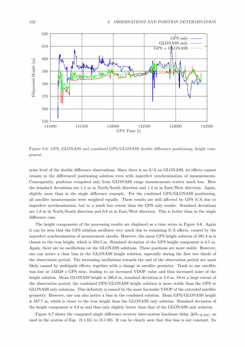
102 8 OBSERVATIONS AND POSITION DETERMINATION
550
560
570
580
590
600
610
620
141000 141500 142000 142500 143000 143500
Elli
psoi
dalH
eigh
t[m
]
GPS Time [s]
GPS onlyGLONASS only
GPS + GLONASS
Figure 8.6: GPS, GLONASS and combined GPS/GLONASS double difference positioning, height com-ponent.
noise level of the double difference observations. Since there is no S/A on GLONASS, its effects cannotremain in the differenced positioning solution even with imperfect synchronization of measurements.Consequently, positions computed only from GLONASS range measurements scatter much less. Herethe standard deviations are 1.4 m in North/South direction and 1.2 m in East/West direction. Again,slightly more than in the single difference example. For the combined GPS/GLONASS positioning,all satellite measurements were weighted equally. These results are still affected by GPS S/A due toimperfect synchronization, but to a much less extent than the GPS only results. Standard deviationsare 1.8 m in North/South direction and 0.8 m in East/West direction. This is better than in the singledifference case.
The height components of the processing results are displayed as a time series in Figure 8.6. Againit can be seen that the GPS solution oscillates very much due to remaining S/A effects, caused by theimperfect synchronization of measurement epochs. However, the mean GPS height solution of 591.3 m isclosest to the true height, which is 594.5 m. Standard deviation of the GPS height component is 6.5 m.Again, there are no oscillations on the GLONASS solutions. These positions are more stable. However,one can notice a clear bias in the GLONASS height solution, especially during the first two thirds ofthe observation period. The increasing oscillations towards the end of the observation period are mostlikely caused by multipath effects, together with a change in satellite geometry. Track to one satellitewas lost at 143328 s GPS time, leading to an increased VDOP value and thus increased noise of theheight solution. Mean GLONASS height is 586.0 m, standard deviation is 3.9 m. Over a large extent ofthe observation period, the combined GPS/GLONASS height solution is more stable than the GPS orGLONASS only solutions. This definitely is caused by the more favorable VDOP of the extended satellitegeometry. However, one can also notice a bias in the combined solution. Mean GPS/GLONASS heightis 587.7 m, which is closer to the true height than the GLONASS only solution. Standard deviation ofthe height component is 3.8 m and thus only slightly better than that of the GLONASS only solution.
Figure 8.7 shows the computed single difference receiver inter-system hardware delay ∆δtUR,HW , asused in the system of Eqs. (8.1.65) to (8.1.69). It can be clearly seen that this bias is not constant. Its
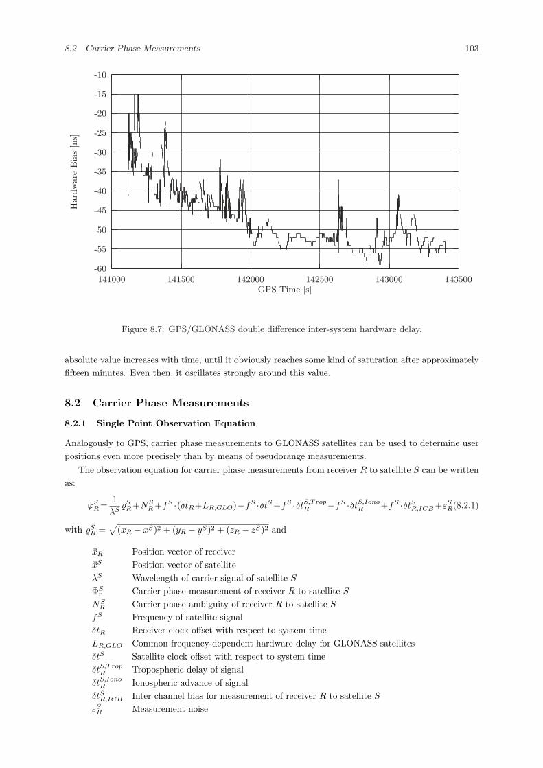
8.2 Carrier Phase Measurements 103
-60
-55
-50
-45
-40
-35
-30
-25
-20
-15
-10
141000 141500 142000 142500 143000 143500
Har
dwar
eB
ias
[ns]
GPS Time [s]
Figure 8.7: GPS/GLONASS double difference inter-system hardware delay.
absolute value increases with time, until it obviously reaches some kind of saturation after approximatelyfifteen minutes. Even then, it oscillates strongly around this value.
8.2 Carrier Phase Measurements
8.2.1 Single Point Observation Equation
Analogously to GPS, carrier phase measurements to GLONASS satellites can be used to determine userpositions even more precisely than by means of pseudorange measurements.
The observation equation for carrier phase measurements from receiver R to satellite S can be writtenas:
ϕSR =
1λS
%SR+NS
R +fS ·(δtR+LR,GLO)−fS ·δtS +fS ·δtS,TropR −fS ·δtS,Iono
R +fS ·δtSR,ICB +εSR(8.2.1)
with %SR =
√(xR − xS)2 + (yR − yS)2 + (zR − zS)2 and
~xR Position vector of receiver~xS Position vector of satelliteλS Wavelength of carrier signal of satellite S
ΦSr Carrier phase measurement of receiver R to satellite S
NSR Carrier phase ambiguity of receiver R to satellite S
fS Frequency of satellite signalδtR Receiver clock offset with respect to system timeLR,GLO Common frequency-dependent hardware delay for GLONASS satellitesδtS Satellite clock offset with respect to system timeδtS,Trop
R Tropospheric delay of signalδtS,Iono
R Ionospheric advance of signalδtSR,ICB Inter channel bias for measurement of receiver R to satellite S
εSR Measurement noise
104 8 OBSERVATIONS AND POSITION DETERMINATION
It should be noted that, due to the dispersive character of the ionosphere, the carrier signal is acceleratedin the ionosphere, contrary to the code signal, which is delayed.
Units in Eq. (8.2.1) are cycles. Scaled to units of length, this equation reads
ΦSR = %S
R +λSNSR + c · (δtR + LR,GLO)− c · δtS + c · δtS,Trop
R − c · δtS,IonoR + c · δtSR,ICB +λSεS
R(8.2.2)
where
c Speed of light in vacuumΦS
R = λSϕSR Carrier phase measurement scaled to distance
Like in the case of the pseudorange observations Eq. (8.1.8), the tropospheric delay δtS,TropR has
to be determined using a suitable model, e.g. a Modified Hopfield model, if possible supported bymeasurements of the actual temperature, air pressure and humidity at the time of observation. Theionospheric acceleration δtS,Iono
R also can be modeled using e.g. the GPS Klobuchar model, adaptedto GLONASS carrier frequencies. This model as described in Section 8.5 for the determination of theionospheric path delay for L1 pseudorange measurements can likewise be applied to the correction ofionospheric acceleration for L1 carrier phase measurements, but with negative sign. Or again, the observercan make use of the free availability of the GLONASS L2 frequency by estimating the ionospheric delayfrom dual frequency code pseudoranges and applying it with negative sign to correct for the carrier phaseacceleration. There are, however, some differences between the ionospheric free linear combinations ofcode pseudoranges and carrier phase measurements. Section 8.5 will treat the ionosphere in more detail.
In Eq. (8.2.2) the frequency-dependent hardware delays LSR are already split into a common part
LR,GLO and the inter-channel biases δtSR,ICD. Like in the case of the pseudorange observation equation(8.1.8), the common part of the hardware delays contributes to the receiver clock error and cannot beseparated from that. But given the low noise of carrier phase observations, the inter-channel biases canno longer be neglected.
In a combined GPS/GLONASS observation scenario, the carrier phase equivalents of Eqs. (8.1.17)and (8.1.18) can be written as
ϕiR =
1λGPS
%iR + N i
R + fGPS · (δtR + LR,GPS)− fGPS · δti + fGPS · δti,TropR − (8.2.3)
fGPS · δti,IonoR + εi
R
ϕjR =
1λj
%jR + N j
R + f j · (δtR + LR,GPS) + f j · δtSys + f j · δtR,HW − f jδtj + (8.2.4)
f j · δtj,TropR − f j · δtj,Iono
R + f j · δtjR,ICB + εjR
in units of cycles or
ΦiR = %i
R + λGPSN iR + c · (δtR + LR,GPS)− c · δti + c · δti,Trop
R − c · δti,IonoR + λGPSεi
R (8.2.5)
ΦjR = %j
R + λjN jR + c · (δtR + LR,GPS) + c · δtSys + c · δtR,HW − c · δtj + c · δtj,Trop
R − (8.2.6)
c · δtj,IonoR + c · δtjR,ICB + λjεj
R
in units of length. i and j denote a GPS and a GLONASS satellite, respectively.As already explained in Section 8.1.1, most combined GPS/GLONASS receivers will use different
hardware to process HF signals from GPS and from GLONASS satellites, even from different GLONASSsatellites to account for the different carrier frequencies. In some cases even different clocks are used forGPS and GLONASS. This may lead to different hardware delays for GPS and GLONASS satellites andeven for individual GLONASS satellites. These different hardware delays appear as the hardware offsetbetween GPS and average GLONASS δtR,HW and as the inter-channel biases δtjR,ICB in Eq. (8.2.6). Inthe form as employed in Eq. (8.2.6), these inter-channel biases are zeroed at the average hardware delayfor GLONASS satellites. The receiver hardware delay between GPS and average GLONASS in the formas employed in Eq. (8.2.6) cannot be separated from the difference in GPS / GLONASS system timesδtSys.
8.2 Carrier Phase Measurements 105
Single point positioning using carrier phase observations has gained no practical importance. Theobservation equations are written here for the sake of completeness and as the basis for the derivationsin the following sections.
8.2.2 Single Difference Positioning
The differencing techniques as introduced in Section 8.1 for pseudorange measurements can also be appliedto carrier phase measurements in order to eliminate error sources from the observations.
Given two observation sites, one reference station R with known coordinates and a user site U , forwhich the coordinates are to be determined, the single difference GLONASS carrier phase observationequation to satellite S reads:
ϕSU − ϕS
R =1λS
%SU −
1λS
%SR + NS
U −NSR + fS · (δtU + LU,GLO)− fS · (δtR + LR,GLO) + (8.2.7)
fS · δtS,TropU − fS · δtS,Trop
R + fS · δtU,ICB − fS · δtSR,ICB + εSU − εS
R
in units of cycles, and
ΦSU − ΦS
R = %SU − %S
R + λSNSU − λSNS
R + c · (δtU + LU,GLO)− c · (δtR + LR,GLO) + (8.2.8)
c · δtS,TropU − c · δtS,Trop
R + c · δtU,ICB − c · δtSR,ICB + λSεSU − λSεS
R
in units of length. The satellite clock error, which is common to both observers, cancels in this singledifference. As already discussed in Section 8.1.2, the influence of the ionosphere will be equal at bothsites for small and medium baselines and therefore cancels, too. But that does not hold true for thetropospheric path delay, which can be different even for nearby stations.
Using the denotation ∗U − ∗R = ∆∗UR for the single difference terms, Eqs. (8.2.7) and (8.2.8)transform to
∆ϕSUR =
1λS
∆%SUR+∆NS
UR+fS ·(∆δtUR+∆LUR,GLO)+fS ·∆δtS,TropUR +fS ·∆δtSUR,ICB+∆εS
UR(8.2.9)
∆ΦSUR =∆%S
UR+λS∆NSUR+c·(∆δtUR+∆LUR,GLO)+c·∆δtS,Trop
UR +c·∆δtSUR,ICB+λS∆εSUR(8.2.10)
Compared to the single difference observation equation for pseudoranges Eq. (8.1.27), Eqs. (8.2.9) and(8.2.10) contain two additional unknowns, the single difference integer ambiguity ∆NS
UR and the singledifference inter-channel bias ∆δtSUR,ICB . These are unknowns specific to each tracked satellite. Togetherwith position and single difference receiver clock error, a system of n carrier phase observations features2n + 4 unknowns. Even with the addition of pseudorange observations to all the tracked satellite, whichwould provide n more measurements and no more unknowns, a system of single difference carrier phaseobservation equations to any number of GLONASS satellites is always underdetermined. The system,however, becomes solvable, if the inter-channel biases are neglected or can be determined in some otherway and thus disappear as unknowns in Eqs. (8.2.9) and (8.2.10). In this case, n + 4 unknowns remain,leaving the system determined with carrier phase and code pseudorange measurements to at least foursatellites.
For combined measurements to a GPS satellite i and a GLONASS satellite j, the single differenceobservation equations can be written as
∆ϕiUR =
1λGPS
∆%iUR + ∆N i
UR + fGPS · (∆δtUR+∆LUR,GPS) + fGPS ·∆δti,TropUR + (8.2.11)
∆εiUR
∆ϕjUR =
1λj
∆%jUR + ∆N j
UR + f j · (∆δtUR+LUR,GPS) + f j ·∆δtUR,HW + (8.2.12)
f j ·∆δtj,TropUR + f j ·∆δtjUR,ICB + ∆εj
UR
106 8 OBSERVATIONS AND POSITION DETERMINATION
in units of cycles or
∆ΦiUR = ∆%i
UR + λGPS∆N iUR + c · (∆δtUR+∆LUR,GPS) + c ·∆δti,Trop
UR + λGPS∆εiUR (8.2.13)
∆ΦjUR = ∆%j
UR + λj∆N jUR + c · (∆δtUR+∆LUR,GPS) + c ·∆δtUR,HW + c ·∆δtj,Trop
UR + (8.2.14)
c ·∆δtjUR,ICB + λj∆εjUR
in units of length.Along with the common satellite clock error and the ionospheric influence, the GPS/GLONASS
system clock offset cancels. As with the GLONASS only case, these equations feature two additionalunknowns when compared to the single difference observation equations for pseudorange measurements.Together with position, single difference receiver clock error and single difference receiver hardware delays,a system of observations to m GPS and n GLONASS satellites provides m + 2n + 5 unknowns. Addingpseudorange measurements provides another m + n observations, but no further unknowns. Thus, with2(m + n) observations and m + 2n + 5 unknowns, the system can be solved for at least 5 observations toGPS satellites.
An example of positioning results using GPS and GLONASS single difference positioning with car-rier phases is shown in Figure 8.8. Positions were computed from data logged by two 3S NavigationR-100/R-101 receivers, which were set up at known locations at the Institute of Geodesy and Naviga-tion. Pseudorange and carrier phase measurements were logged every second for approximately one houreach, of which some forty minutes were common to both receivers. One of these receivers was used asreference station, the other was treated as the user station. Its position was determined in this example.Observation epochs at both receivers were not exactly synchronized. The data are the same as the dataalready used for the pseudorange positioning example. The plot shows the deviation from the knownlocation of the antenna of the user station in the horizontal plane. GPS positions were computed fromL1 carrier phase measurements and raw L1 C/A-code pseudorange measurements. GLONASS positionswere computed from dual-frequency carrier phase measurements and raw dual-frequency P-code measure-ments. Wherever possible, the ionospheric free linear combinations of the code observables were formed.These observables used are not really identical for GPS and GLONASS, but with dual-frequency mea-surements readily available on GLONASS, the best possible results for each system are determined. Theinter-channel biases ∆δtSUR,ICB for the GLONASS satellites have been neglected. GLONASS satellitepositions were converted from PZ-90 to WGS84 using the transformation according to (Roßbach et al.,1996). Carrier phase ambiguities have not been fixed. The pseudorange observations have been includedin the positioning to increase the number of observations, even though these observations are much noisierthan the carrier phase measurements and thus may adversely affect the accuracy of the results.
Figure 8.8 shows the deviations from the known position in the horizontal plane. The converging ofthe Kalman filter towards the true position is clearly visible. Figure 8.9 shows the time series of the 3Ddeviation from the true position. The GPS only solution exhibits some amount of oscillations, probablydue to remaining S/A effects, because the observation epochs at reference and user stations were notexactly synchronized. This solution converges towards the true position only very late. The GLONASSonly and the combined GPS/GLONASS solutions converge much earlier and then remain steady at apoint approximately 60 mm from the true position. The combined solution converges even earlier thanthe GLONASS solution.
8.2.3 Double Difference Positioning
Using the denotation ∆ ∗SUR −∆∗r
UR = ∇∆∗SrUR, differencing two single difference observations at the
same sites to two different satellites yields the double difference observation
∇∆ϕSrUR =
1λS
∆%SUR −
1λr
∆%rUR +∇∆NSr
UR +(fS − fr
) · (∆δtUR + ∆LUR,GLO) + (8.2.15)
fS ·∆δtS,TropUR − fr ·∆δr,Trop
UR + fS ·∆δtSUR,ICB − fr ·∆δtrUR,ICB +∇∆εSrUR
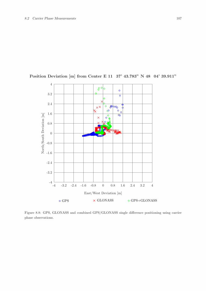
8.2 Carrier Phase Measurements 107
Position Deviation [m] from Center E 11� 37’ 43.783” N 48� 04’ 39.911”
◦ GPS × GLONASS ¦ GPS+GLONASS
East/West Deviation [m]
-4 -3.2 -2.4 -1.6 -0.8 0 0.8 1.6 2.4 3.2 4
Nor
th/S
outh
Dev
iati
on[m
]
-4
-3.2
-2.4
-1.6
-0.8
0
0.8
1.6
2.4
3.2
4
◦◦
◦◦◦
◦◦◦
◦◦◦◦◦◦◦◦◦◦
◦◦◦◦◦◦◦◦◦◦◦◦◦◦◦◦◦◦◦◦◦◦
◦◦◦◦◦◦◦◦◦◦◦◦◦◦◦◦◦◦◦◦◦◦◦◦◦◦◦◦◦◦◦◦◦◦◦◦◦◦◦◦◦◦◦◦◦◦◦◦◦◦◦◦◦◦◦◦◦◦◦◦◦◦◦◦◦◦◦◦◦◦◦◦◦◦◦◦◦◦◦◦◦◦◦◦◦◦◦◦◦◦◦◦◦◦◦◦◦◦◦◦◦◦◦◦◦◦◦◦◦◦◦◦◦◦◦◦◦◦◦◦◦◦◦◦◦◦◦◦◦◦◦◦◦◦◦◦◦◦◦◦◦◦◦◦◦◦◦◦◦◦◦◦◦◦◦◦◦◦◦◦◦◦◦◦◦◦◦◦◦◦◦◦◦◦◦◦◦◦◦◦◦◦◦◦◦◦◦◦◦◦◦◦◦◦◦◦◦◦◦◦◦◦◦◦◦◦◦◦◦
◦◦◦◦◦◦◦◦◦◦◦◦◦◦◦◦◦◦◦◦◦◦◦◦◦◦◦◦◦◦◦◦◦◦◦◦◦◦◦◦◦◦◦◦◦◦◦◦◦◦◦◦◦◦◦◦◦◦◦◦◦◦◦◦◦◦◦◦◦◦◦◦◦◦◦◦◦◦◦◦◦◦◦◦◦◦◦◦◦◦◦◦◦◦◦◦◦◦◦◦◦◦◦◦◦◦◦◦◦◦◦◦◦◦◦◦◦◦◦◦◦◦◦◦◦◦◦◦◦◦◦◦◦◦◦◦◦◦◦◦◦◦◦◦◦◦◦◦◦◦◦◦◦◦◦◦◦◦◦◦◦◦◦◦◦◦◦◦◦◦◦◦◦◦◦◦◦◦◦◦◦◦◦◦◦◦◦◦◦◦◦◦◦◦◦◦◦◦◦◦◦◦◦◦◦◦◦◦◦◦◦◦◦◦◦◦◦◦◦◦◦◦◦◦◦◦◦◦◦◦◦◦◦◦◦◦◦◦◦◦◦◦◦◦◦◦◦◦◦◦◦◦◦◦◦◦◦◦◦◦◦◦◦◦◦◦◦◦◦◦◦◦◦◦◦◦◦◦◦◦◦◦◦◦◦◦◦◦◦◦◦◦◦◦◦◦◦◦◦◦◦◦◦◦◦◦◦◦◦◦◦◦◦◦◦◦◦◦◦◦◦◦◦◦◦◦◦◦◦◦◦◦◦◦◦◦◦◦◦◦◦◦◦◦◦◦◦◦◦◦◦◦◦◦◦◦◦◦◦◦◦◦◦◦◦◦◦◦◦◦◦◦◦◦◦◦◦◦◦◦◦◦◦◦◦◦◦◦◦◦◦◦◦◦◦◦◦◦◦◦◦◦◦◦◦◦◦◦◦◦◦◦◦◦◦◦◦◦◦◦◦◦◦◦◦◦◦◦◦◦◦◦◦◦◦◦◦◦◦◦◦◦◦◦◦◦◦◦◦◦◦◦◦◦◦◦◦◦◦◦◦◦◦◦◦◦◦◦◦◦◦◦◦◦◦◦◦◦◦◦◦◦◦◦◦◦◦◦◦◦◦◦◦◦◦◦◦◦◦◦◦◦◦◦◦◦◦◦◦◦◦◦◦◦◦◦◦◦◦◦◦◦◦◦◦◦◦◦◦◦◦◦◦◦◦◦◦◦◦◦◦◦◦◦◦◦◦◦◦◦◦◦◦◦◦◦◦◦◦◦◦◦◦◦◦◦◦◦◦◦◦◦◦◦◦◦◦◦◦◦◦◦◦◦◦◦◦◦◦◦◦◦◦◦◦◦◦◦◦◦◦◦◦◦◦◦◦◦◦◦◦◦◦◦◦◦◦◦◦◦◦◦◦◦◦◦◦◦◦◦◦◦◦◦◦◦◦◦◦◦◦◦◦◦◦◦◦◦◦◦◦◦◦◦◦◦◦◦◦◦◦◦◦◦◦◦◦◦◦◦◦◦◦◦◦◦◦◦◦◦◦◦◦◦◦◦◦◦◦◦◦◦◦◦◦◦◦◦◦◦◦◦◦◦◦◦◦◦◦◦◦◦◦◦◦◦◦◦◦◦◦◦◦◦◦◦◦◦◦◦◦◦◦◦◦◦◦◦◦◦◦◦◦◦◦◦◦◦◦◦◦◦◦◦◦◦◦◦◦◦◦◦◦◦◦◦◦◦◦◦◦◦◦◦◦◦◦◦◦◦◦◦◦◦◦◦◦◦◦◦◦◦◦◦◦◦◦◦◦◦◦◦◦◦◦◦◦◦◦◦◦◦◦◦◦◦◦◦◦◦◦◦◦◦◦◦◦◦◦◦◦◦◦◦◦◦◦◦◦◦◦◦◦◦◦◦◦◦◦◦◦◦◦◦◦◦◦◦◦◦◦◦◦◦◦◦◦◦◦◦◦◦◦◦◦◦◦◦◦◦◦◦◦◦◦◦◦◦◦◦◦◦◦◦◦◦◦◦◦◦◦◦◦◦◦◦◦◦◦◦◦◦◦◦◦◦◦◦◦◦◦◦◦◦◦◦◦◦◦◦◦◦◦◦◦◦◦◦◦◦◦◦◦◦◦◦◦◦◦◦◦◦◦◦◦◦◦◦◦◦◦◦◦◦◦◦◦◦◦◦◦◦◦◦◦◦◦◦◦◦◦◦◦◦◦◦◦◦◦◦◦◦◦◦◦◦◦◦◦◦◦◦◦◦◦◦◦◦◦◦◦◦◦◦◦◦◦◦◦◦◦◦◦◦◦◦◦◦◦◦◦◦◦◦◦◦◦◦◦◦◦◦◦◦◦◦◦◦◦◦◦◦◦◦◦◦◦◦◦◦◦◦◦◦◦◦◦◦◦◦◦◦◦◦◦◦◦◦◦◦◦◦◦◦◦◦◦◦◦◦◦◦◦◦◦◦◦◦◦◦◦◦◦◦◦◦◦◦◦◦◦◦◦◦◦◦◦◦◦◦◦◦◦◦◦◦◦◦◦◦◦◦◦◦◦◦◦◦◦◦◦◦◦◦◦◦◦◦◦◦◦◦◦◦◦◦◦◦◦◦◦◦◦◦◦◦◦◦◦◦◦◦◦◦◦◦◦◦◦◦◦◦◦◦◦◦◦◦◦◦◦◦◦◦◦◦◦◦◦◦◦◦◦◦◦◦◦◦◦◦◦◦◦◦◦◦◦◦◦◦◦◦◦◦◦◦◦◦◦◦◦◦◦◦◦◦◦◦◦◦
×××××
×× ××
××××××××× ××××××××××××××××××××××××××××××××××××××××××××××××××××××××××××××××××××××××××××××××××××××××××××××××××××××××××××××××××××××××××××××××××××××××××××××××××××××××××××××××××××××××××××××××××××××××××××××××××××××××××××××××××××××××××××××××××××××××××××××××××××××××××××××××××××××××××××××××××××××××××××××××××××××××××××××××××××××××××××××××××××××××××××××××××××××××××××××××××××××××××××××××××××××××××××××××××××××××××××××××××××××××××××××××××××××××××××××××××××××××××××××××××××××××××××××××××××××××××××××××××××××××××××××××××××××××××××××××××××××××××××××××××××××××××××××××××××××××××××××××××××××××××××××××××××××××××××××××××××××××××××××××××××××××××××××××××××××××××××××××××××××××××××××××××××××××××××××××××××××××××××××××××××××××××××××××××××××××××××××××××××××××××××××××××××××××××××××××××××××××××××××××××××××××××××××××××××××××××××××××××××××××××××××××××××××××××××××××××××××××××××××××××××××××××××××××××××××××××××××××××××××××××××××××××××××××××××××××××××××××××××××××××××××××××××××××××××××××××××××××××××××××××××××××××××××××××××××××××××××××××××××××××××××××××××××××××××××××××××××××××××××××××××××××××××××××××××××××××××××××××××××××××××××××××××××××××××××××××××××××××××××××××××××××××××××××××××××××××××××××××××××××××××××××
¦¦¦¦¦
¦¦¦
¦¦¦¦¦¦¦¦¦¦¦¦¦¦¦¦¦¦¦¦¦¦¦¦¦¦¦¦¦¦¦¦¦¦¦¦¦¦¦¦¦¦¦¦¦¦¦¦¦¦¦¦¦¦¦¦¦¦¦¦¦¦¦¦¦
¦¦¦¦¦¦¦¦¦¦¦¦¦¦¦¦¦¦¦¦¦¦¦¦¦¦¦¦¦¦¦¦¦¦¦¦¦¦¦¦¦¦¦¦¦¦¦¦¦¦¦¦¦¦¦¦¦¦¦¦¦¦¦¦¦¦¦¦¦¦¦¦¦¦¦¦¦¦¦¦¦¦¦¦¦¦¦¦¦¦¦¦¦¦¦¦¦¦¦¦¦¦¦¦¦¦¦¦¦¦¦¦¦¦¦¦¦¦¦¦¦¦¦¦¦¦¦¦¦¦¦¦¦¦¦¦¦¦¦¦¦¦¦¦¦¦¦¦¦¦¦¦¦¦¦¦¦¦¦¦¦¦¦¦¦¦¦¦¦¦¦¦¦¦¦¦¦¦¦¦¦¦¦¦¦¦¦¦¦¦¦¦¦¦¦¦¦¦¦¦¦¦¦¦¦¦¦¦¦¦¦¦¦¦¦¦¦¦¦¦¦¦¦¦¦¦¦¦¦¦¦¦¦¦¦¦¦¦¦¦¦¦¦¦¦¦¦¦¦¦¦¦¦¦¦¦¦¦¦¦¦¦¦¦¦¦¦¦¦¦¦¦¦¦¦¦¦¦¦¦¦¦¦¦¦¦¦¦¦¦¦¦¦¦¦¦¦¦¦¦¦¦¦¦¦¦¦¦¦¦¦¦¦¦¦¦¦¦¦¦¦¦¦¦¦¦¦¦¦¦¦¦¦¦¦¦¦¦¦¦¦¦¦¦¦¦¦¦¦¦¦¦¦¦¦¦¦¦¦¦¦¦¦¦¦¦¦¦¦¦¦¦¦¦¦¦¦¦¦¦¦¦¦¦¦¦¦¦¦¦¦¦¦¦¦¦¦¦¦¦¦¦¦¦¦¦¦¦¦¦¦¦¦¦¦¦¦¦¦¦¦¦¦¦¦¦¦¦¦¦¦¦¦¦¦¦¦¦¦¦¦¦¦¦¦¦¦¦¦¦¦¦¦¦¦¦¦¦¦¦¦¦¦¦¦¦¦¦¦¦¦¦¦¦¦¦¦¦¦¦¦¦¦¦¦¦¦¦¦¦¦¦¦¦¦¦¦¦¦¦¦¦¦¦¦¦¦¦¦¦¦¦¦¦¦¦¦¦¦¦¦¦¦¦¦¦¦¦¦¦¦¦¦¦¦¦¦¦¦¦¦¦¦¦¦¦¦¦¦¦¦¦¦¦¦¦¦¦¦¦¦¦¦¦¦¦¦¦¦¦¦¦¦¦¦¦¦¦¦¦¦¦¦¦¦¦¦¦¦¦¦¦¦¦¦¦¦¦¦¦¦¦¦¦¦¦¦¦¦¦¦¦¦¦¦¦¦¦¦¦¦¦¦¦¦¦¦¦¦¦¦¦¦¦¦¦¦¦¦¦¦¦¦¦¦¦¦¦¦¦¦¦¦¦¦¦¦¦¦¦¦¦¦¦¦¦¦¦¦¦¦¦¦¦¦¦¦¦¦¦¦¦¦¦¦¦¦¦¦¦¦¦¦¦¦¦¦¦¦¦¦¦¦¦¦¦¦¦¦¦¦¦¦¦¦¦¦¦¦¦¦¦¦¦¦¦¦¦¦¦¦¦¦¦¦¦¦¦¦¦¦¦¦¦¦¦¦¦¦¦¦¦¦¦¦¦¦¦¦¦¦¦¦¦¦¦¦¦¦¦¦¦¦¦¦¦¦¦¦¦¦¦¦¦¦¦¦¦¦
Figure 8.8: GPS, GLONASS and combined GPS/GLONASS single difference positioning using carrierphase observations.
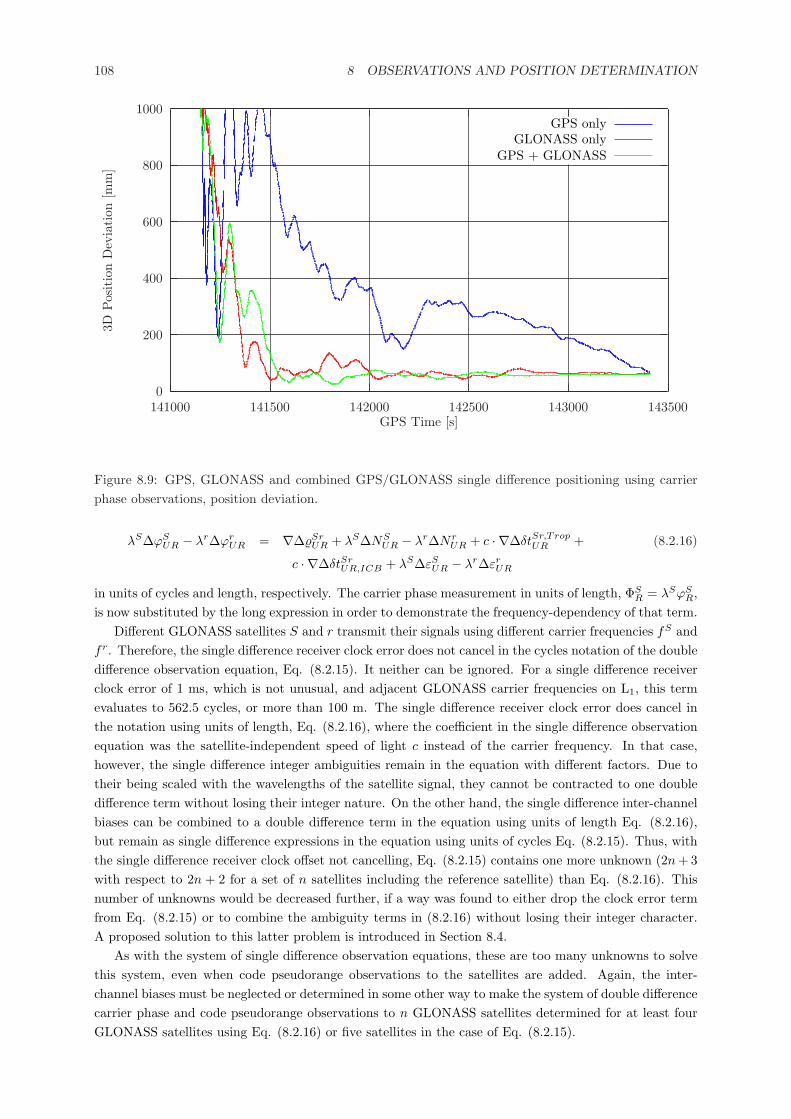
108 8 OBSERVATIONS AND POSITION DETERMINATION
0
200
400
600
800
1000
141000 141500 142000 142500 143000 143500
3DPos
itio
nD
evia
tion
[mm
]
GPS Time [s]
GPS onlyGLONASS only
GPS + GLONASS
Figure 8.9: GPS, GLONASS and combined GPS/GLONASS single difference positioning using carrierphase observations, position deviation.
λS∆ϕSUR − λr∆ϕr
UR = ∇∆%SrUR + λS∆NS
UR − λr∆NrUR + c · ∇∆δtSr,Trop
UR + (8.2.16)
c · ∇∆δtSrUR,ICB + λS∆εS
UR − λr∆εrUR
in units of cycles and length, respectively. The carrier phase measurement in units of length, ΦSR = λSϕS
R,is now substituted by the long expression in order to demonstrate the frequency-dependency of that term.
Different GLONASS satellites S and r transmit their signals using different carrier frequencies fS andfr. Therefore, the single difference receiver clock error does not cancel in the cycles notation of the doubledifference observation equation, Eq. (8.2.15). It neither can be ignored. For a single difference receiverclock error of 1 ms, which is not unusual, and adjacent GLONASS carrier frequencies on L1, this termevaluates to 562.5 cycles, or more than 100 m. The single difference receiver clock error does cancel inthe notation using units of length, Eq. (8.2.16), where the coefficient in the single difference observationequation was the satellite-independent speed of light c instead of the carrier frequency. In that case,however, the single difference integer ambiguities remain in the equation with different factors. Due totheir being scaled with the wavelengths of the satellite signal, they cannot be contracted to one doubledifference term without losing their integer nature. On the other hand, the single difference inter-channelbiases can be combined to a double difference term in the equation using units of length Eq. (8.2.16),but remain as single difference expressions in the equation using units of cycles Eq. (8.2.15). Thus, withthe single difference receiver clock offset not cancelling, Eq. (8.2.15) contains one more unknown (2n + 3with respect to 2n + 2 for a set of n satellites including the reference satellite) than Eq. (8.2.16). Thisnumber of unknowns would be decreased further, if a way was found to either drop the clock error termfrom Eq. (8.2.15) or to combine the ambiguity terms in (8.2.16) without losing their integer character.A proposed solution to this latter problem is introduced in Section 8.4.
As with the system of single difference observation equations, these are too many unknowns to solvethis system, even when code pseudorange observations to the satellites are added. Again, the inter-channel biases must be neglected or determined in some other way to make the system of double differencecarrier phase and code pseudorange observations to n GLONASS satellites determined for at least fourGLONASS satellites using Eq. (8.2.16) or five satellites in the case of Eq. (8.2.15).
8.2 Carrier Phase Measurements 109
Analogously to the pseudorange observation equations, for the double differenced carrier phase ob-servation equations in a combined GPS/GLONASS scenario with a GPS satellite i and a GLONASSsatellite j three different cases must be distinguished, depending on the reference satellite:
1. The reference satellite rGPS is a GPS satellite.
The double difference observation equations can be written as
∇∆ϕirGP S
UR =1
λGPS∇∆%irGP S
UR +∇∆N irGP S
UR + fGPS · ∇∆δtirGP S ,Trop
UR +∇∆εirGP S
UR (8.2.17)
∇∆ϕjrGP S
UR =1λj
∆%jUR−
1λGPS
∆%rGP S
UR +∇∆N jrGP S
UR +(f j−fGPS
) · (∆δtUR+∆LUR,GPS)+
f j ·∆δtUR,HW +f j ·∆δtj,TropUR −fGPS ·∆δtr
GP S ,TropUR + (8.2.18)
f j ·∆δtjUR,ICB+∇∆εjUR
in units of cycles or
λGPS∇∆ϕirGP S
UR = ∇∆%irGP S
UR +λGPS∇∆N irGP S
UR +c·∇∆δtirGP S ,Trop
UR +λGPS∇∆εirGP S
UR (8.2.19)
λj∆ϕjUR − λGPS∆ϕrGP S
UR = ∇∆%jrGP S
UR + λj∆N jUR − λGPS∆NrGP S
UR + c ·∆δtUR,HW +
c · ∇∆δtjrGP S ,TropUR + c ·∆δtjUR,ICB + λj∆εj
UR − (8.2.20)
λGPS∆εrGP S
UR
in units of length, respectively.
Of course, the GPS/GPS double difference reads like what one would expect from GPS only pro-cessing. The single difference receiver clock offset, common to both satellites, cancels, and all othersingle difference terms can be combined to double difference expressions. For the GLONASS/GPSdouble difference, as already observed in the GLONASS only scenario, due to the different fre-quencies of the participating satellites either the single difference receiver clock offset, combinedwith the GPS hardware delay, ∆δtUR + ∆LUR,GPS does not cancel (in the cycles notation) or thetwo single difference integer ambiguities cannot be contracted to one double difference term (in thelength notation). In addition, the single difference receiver inter-system hardware delay ∆δtUR,HW
remains in the mixed GLONASS/GPS double difference, as already observed in the pseudorangedouble difference processing, as well as the single difference receiver inter-channel biases.
For a scenario with m GPS and n GLONASS satellites, the set of observation equations containsm + 2n + 4 unknowns.
2. The reference satellite rGLO is a GLONASS satellite.
The double difference observation equations can in that case be written as
∇∆ϕirGLO
UR =1
λGPS∆%i
UR −1
λrGLO ∆%rGLO
UR +∇∆N irGLO
UR +(fGPS − frGLO
)· (∆δtUR + ∆LUR,GPS)− frGLO ·∆δtUR,HW + (8.2.21)
fGPS ·∆δti,TropUR − frGLO ·∆δtr
GLO,TropUR − frGLO ·∆δtr
GLO
UR,ICB +∇∆εiUR
∇∆ϕjrGLO
UR =1λj
∆%jUR −
1λrGLO ∆%rGLO
UR +∇∆N jrGLO
UR +(f j − frGLO
)· (∆δtUR + ∆LUR,GPS) + (8.2.22)
(f j − frGLO
)·∆δtUR,HW + f j ·∆δtj,Trop
UR − frGLO ·∆δtrGLO,Trop
UR +
f j ·∆δtjUR,ICB − frGLO ·∆δtrGLO
UR,ICB +∇∆εjUR
110 8 OBSERVATIONS AND POSITION DETERMINATION
in units of cycles or
λGPS∆ϕiUR − λrGLO
∆ϕrGLO
UR = ∇∆%irGLO
UR + λGPS∆N iUR − λrGLO
∆NrGLO
UR −c ·∆δtUR,HW + c · ∇∆δtir
GLO,TropUR − (8.2.23)
c ·∆δtrGLO
UR,ICB + λGPS∆εiUR − λrGLO
∆εrGLO
UR
λj∆ϕjUR − λrGLO
∆ϕrGLO
UR = ∇∆%jrGLO
UR + λj∆N jUR − λrGLO
∆NrGLO
UR +
c · ∇∆δtjrGLO,TropUR + c · ∇∆δtjrGLO
UR,ICB + (8.2.24)
λj∆εjUR − λrGLO
∆εrGLO
UR
in units of length, respectively
The GPS/GLONASS double difference is equivalent to the GLONASS/GPS double difference fromabove, but with inverse signs. For the GLONASS/GLONASS double difference, again due tothe different frequencies of the participating satellites the single difference receiver clock offset∆δtUR + ∆LUR,GPS does not cancel in the cycles notation, nor does the single difference receiverinter-system hardware delay ∆δtUR,HW . They both cancel in the notation using units of length.But here again, both single difference integer ambiguities remain in the equation, with differentfactors. This turns the other way around for the single difference inter-channel biases. They can becombined to one double difference term in the equation using units of length, but remain as singledifference terms with different factors in the equation using units of cycles.
For a scenario with m GPS and n GLONASS satellites, the set of observation equations containsm + 2n + 4 unknowns.
3. Separate reference satellites rGPS for GPS and rGLO for GLONASS
In that case the double difference observation equations become
∇∆ϕirGP S
UR =1
λGPS∇∆%irGP S
UR +∇∆N irGP S
UR + fGPS · ∇∆δtirGP S ,Trop
UR +∇∆εirGP S
UR (8.2.25)
∇∆ϕjrGLO
UR =1λj
∆%jUR −
1λrGLO ∆%rGLO
UR +∇∆N jrGLO
UR +(f j−frGLO
)· (∆δtUR + ∆LUR,GPS) +
(f j−frGLO
)·∆δtUR,HW +
f j ·∆δtj,TropUR − frGLO ·∆δtr
GLO,TropUR + (8.2.26)
f j ·∆δtjUR,ICB − frGLO ·∆δtrGLO
UR,ICB +∇∆εjUR
in units of cycles or
λGPS∇∆ϕirGP S
UR = ∇∆%irGP S
UR +λGPS∇∆N irGP S
UR +c·∇∆δtirGP S ,Trop
UR +λGPS∇∆εirGP S
UR (8.2.27)
λj∆ϕjUR − λrGLO
∆ϕrGLO
UR = ∇∆%jrGLO
UR + λj∆N jUR − λrGLO
∆NrGLO
UR +
c · ∇∆δtjrGLO,TropUR + c · ∇∆δtjrGLO
UR,ICB + (8.2.28)
λj∆εjUR − λrGLO
∆εrGLO
UR
in units of length, respectively.
This is the combination of the GPS/GPS and GLONASS/GLONASS double differences of the previ-ous two cases. In the GPS/GPS double difference, the single difference receiver clock offset, commonto both satellites, cancels, and all other single difference terms can be combined to double differenceexpressions. In the GLONASS/GLONASS double difference, again due to the different frequenciesof the participating satellites the single difference receiver clock offset ∆δtUR +∆LUR,GPS does notcancel in the cycles notation, nor does the single difference receiver inter-system hardware delay
8.3 GLONASS and GPS/GLONASS Carrier Phase Positioning 111
∆δtUR,HW . They both cancel in the notation using units of length. But here again, both singledifference integer ambiguities remain in the equation, with different factors. This turns the otherway around for the single difference inter-channel biases. They can be combined to one doubledifference term in the equation using units of length, but remain as single difference terms withdifferent factors in the equation using units of cycles.
For a scenario with m GPS and n GLONASS satellites, the set of observation equations containsm+2n+3 unknowns in the formulation in units of cycles and m+2n+1 unknowns in the formulationin units of length. Whereas the formulation using cycles is equivalent to the previous two cases(one less unknown, but also one more observation sacrificed in the differencing), the length notationoffers a clear advantage with regard to the number of unknowns. Here, both the single differencereceiver clock offset ∆δtUR + ∆LUR,GPS and the single difference receiver inter-system hardwaredelay ∆δtUR,HW cancel.
8.3 GLONASS and GPS/GLONASS Carrier Phase Positioning
The different carrier frequencies of the GLONASS satellites cause two major problems when using GLO-NASS carrier phase observations for precise positioning:
• different, frequency-dependent hardware delays in the receiver, and
• either the ambiguities losing their integer nature or the receiver clock errors not cancelling in doubledifference positioning.
Different groups of scientists proposed different methods to treat GLONASS carrier phase observationsin order to tackle these problems, either simultaneously or separately.
8.3.1 Floating GLONASS Ambiguities
Landau et al. (Landau and Vollath, 1996) summarize the integer ambiguities and the frequency-dependentdelays into one non-integer term per satellite and confines to floating GLONASS ambiguities. In combinedGPS/GLONASS scenarios, these GLONASS ambiguities serve only to support fixing of the GPS integerambiguities. When analyzing GPS/GLONASS data, the solution converges far faster than for GPS dataalone. The reliability of the integer fix, quantified in the ratio of the sum of the squared residuals forthe best and second best solution, is also improved by a factor of around 3, when GLONASS satellitesare included in the position determination. The combined number of GPS and GLONASS satellites mayeven allow to obtain very precise positioning solutions without any ambiguity fix at all.
8.3.2 Single Difference Positioning and Receiver Calibration
Daly et al. (Raby and Daly, 1993; Walsh and Daly, 1996) suggest a careful calibration of GLONASSreceivers prior to use in order to determine the hardware delays. Since these delays may also dependon receiver temperature, this calibration should be performed at different temperatures. In a combinedGPS/GLONASS scenario, it is thinkable to first obtain an accurate position fix from GPS measurementsalone for a static receiver. This position fix could then be used to calibrate initial GLONASS hardwaredelays. As long as lock is maintained to at least four GPS satellites, GLONASS measurement errors canbe monitored. If lock is kept to less than four GPS satellites, the most recent calibration values (andperhaps a model for their change in time) will be used. Combined GPS/GLONASS positioning is thenpossible. This technique is especially useful for surveying in sites with lots of obstructions, e.g. openpit mines. Initialization can be performed outside the mine, with a sufficient number of GPS satellitesavailable, before entering the pit.
Regarding the ambiguities, (Walsh and Daly, 1996) avoid the GLONASS double difference carrierphase observations and confine to single differences. This enables fixing the ambiguities to integer values,
112 8 OBSERVATIONS AND POSITION DETERMINATION
at the expense of additionally having to estimate the receiver clock biases. These clock biases can becomputed from pseudorange measurements. These are, however, less precise than the carrier phasemeasurements. After initialization of the GLONASS biases, correct fixing of the integer ambiguities ispossible faster than with GPS alone.
8.3.3 Scaling to a Common Frequency
In order to eliminate the receiver clock errors from the double difference carrier phase observation equationin cycles notation, Leick et al. (Leick et al., 1995) scale the GLONASS carrier phase observations toa common frequency. They choose the mean frequency in the classical range of frequency numbersn = 1 . . . 24:
f i = fi(n = 12.5)
with i = 1, 2 for the L1 and L2 frequencies, respectively, as this common frequency. This way, for allGLONASS satellites S the inequality
0.9959 <f i
fS< 1.0041
holds, at least for the classical range of frequency numbers.The scaled carrier phase observation equation from receiver R to GLONASS satellite S in units of
cycles Eq. (8.2.1) then reads:
ϕSR =
f
fSϕS
R
=f
c%S
R +f
fSNS
R + f · (δtR+LR,GLO)− f · δtS + f · δtS,TropR − f · δtS,Iono
R + (8.3.1)
f · δtSR,ICB +f
fSεSR
Forming a single difference between user receiver U and reference receiver R, the satellite clock errorand for short baselines also the ionospheric influence cancel:
∆ϕSUR =
f
c∆%S
UR +f
fS∆NS
UR + f · (∆δtUR + ∆LUR,GLO) + f ·∆δtS,TropUR + (8.3.2)
f ·∆δtSUR,ICB +f
fS∆εS
UR
and the double differenced observation equation between satellite S and reference satellite r then reads:
∇∆ϕSrUR =
f
fS
(ϕS
U − ϕSR
)− f
fr(ϕr
U − ϕrR)
=f
c∇∆%Sr
UR +f
fS∆NS
UR −f
fr∆Nr
UR + f · ∇∆δtSr,TropUR + f · ∇∆δtSr
UR,ICB + (8.3.3)
f
fS∆εS
UR −f
fr∆εr
UR
The single difference receiver clock offsets, combined with the hardware delay, ∆δtUR+∆LUR,GLO cancels,as was intended by the scaling of the carrier phase observation equation. However, due to the scaling, thesingle difference ambiguities now cannot be contracted to a double difference term, without losing theirinteger nature. In this respect, Eq. (8.3.3) is equivalent to the unscaled double difference observationequation in units of length, Eq. (8.2.16).
To overcome this problem of not being able to contract the single difference ambiguities to a doubledifference term, (Leick et al., 1995) further introduce an approximate value for the single difference carrierphase ambiguity to the reference satellite r such that:
∆NrUR = ∆Nr
UR,0 + dNrUR (8.3.4)
8.3 GLONASS and GPS/GLONASS Carrier Phase Positioning 113
Substituting Eq. (8.3.4) into Eq. (8.3.3) yields:
∇∆ϕSrUR =
f
c∇∆%Sr
UR +f
fS∆NS
UR −f
fr∆Nr
UR,0 −f
frdNr
UR + f · ∇∆δtSr,TropUR + (8.3.5)
f · ∇∆δtSrUR,ICB +
f
fS∆εS
UR −f
fr∆εr
UR
The amendment to this approximate value together with the single difference ambiguity to the refer-ence satellite S can now be contracted to a new double difference term:
∇∆ϕSrUR =
f
c∇∆%Sr
UR +f
fS∇∆NSr
UR −f
fr∆Nr
UR,0 + f · ∇∆δtSr,TropUR + (8.3.6)
f · ∇∆δtSrUR,ICB +
f
fSdNr
UR −f
frdNr
UR +f
fS∆εS
UR −f
fr∆εr
UR
with
∇∆NSrUR = ∆NS
UR − dNrUR
The approximate value for the single difference integer ambiguity ∆NrUR,0 is determined from pseu-
dorange measurements. The remaining amendment terms(
f
fS− f
fs
)· dNr
UR
are of small magnitude, since∣∣∣∣
f
fS− f
fs
∣∣∣∣ <1
124
and the amendment dNrUR itself is considered small. These terms are regarded as model error and treated
as additional noise in Eq. (8.3.6).Since Eq. (8.3.3) is very similar to the double difference observation equation in units of length, Eq.
(8.2.16), splitting of the single difference integer ambiguity to the reference satellite ∆NrUR can also be
applied to this latter equation. The double difference equation in units of length then reads
λS∆ϕSUR − λr∆ϕr
UR = ∇∆%SrUR + λS∇∆NSr
UR − λr∆NrUR,0 + c · ∇∆δtSr,Trop
UR + (8.3.7)
c · ∇∆δtSrUR,ICB + λSdNr
UR − λrdNrUR + λS∆εS
UR − λr∆εrUR
In this case, |λS − λr| < 0.0015 m(Leick et al., 1995) did not make any attempt to calibrate the inter-channel biases δtSr
UR,ICB in Eq.(8.3.6).
8.3.4 Iterative Ambiguity Resolution
(Habrich et al., 1999; Habrich, 1999) suggest an iterative solution of the GLONASS double differenceambiguities, based on the single difference observation equations:
1. In a first step the normal equation system for single difference phase observations is set up. Forobservations to n satellites, there are n single difference equations – assuming single frequencyobservations only.
2. These equations are enhanced by an a priori constraint or by code observations to remove thesingularity of the system.
3. The system of single difference equations system is solved, and the single difference ambiguities areestimated as real values.
114 8 OBSERVATIONS AND POSITION DETERMINATION
4. All possible double difference ambiguities∇∆N ijkl are computed using combinations of the estimated
single difference ambiguities ∆N ikl, ∆N j
kl. Along with these double difference ambiguities, theirformal errors are estimated from the covariance matrix Q of the single difference solution. Theseformal errors are computed as eij = ς0
√Qii − 2Qij + Qjj , with the a posteriori variance factor
ς20 . The formal errors are highly correlated with the difference in wavelength ∆λij of the satellites
involved in the double difference. The smaller the wavelength difference, the smaller the formalerror.
5. The double difference combination with the smallest formal error is then fixed to an integer number.
6. With one double difference fixed, one of the two single difference ambiguities involved in formingthis double difference combination may then be eliminated from the normal equation system. Theobservation system of single difference equations is now regular, even without constraints or codeobservations.
The iterative ambiguity resolution is then continued with step 3, the solution of the single differenceobservation equations. This way, n − 1 single difference ambiguities may be eliminated from theobservation equation.
7. Finally, the remaining single difference ambiguity is fixed to an integer number on the single differ-ence level.
This method of GLONASS ambiguity resolution is applicable for short and long baselines. But it mayonly be used in post processing mode, evaluating data of long observation sessions. Thus, this methodis suited for e.g. analysis of IGEX-98 data. But it is not suited for applications that require fast (”rapidstatic” or ”on-the-fly”) ambiguity determination. It neither can be applied to any form of navigation.
8.4 A Proposed Solution to the Frequency Problem
The double difference carrier phase observations between stations U and R to satellites S and r in unitsof length can be written as (cf. Eq. (8.2.16))
λS∆ϕSUR − λr∆ϕr
UR = ∇∆%SrUR + λS∆NS
UR − λr∆NrUR + λS∆εS
UR − λr∆εrUR (8.4.1)
Compared to Eq. (8.2.16), the tropospheric path delay and the inter-channel bias have been neglected.These terms do not contribute to the purpose of demonstrating a proposed solution to the problem ofhaving the single difference integer ambiguities in the double difference observation equation.
Given two GPS satellites with identical signal wavelengths λS = λr = λGPS , Eq. (8.4.1) simplifies to
λGPS∇∆ϕSrUR = ∇∆%Sr
UR + λGPS∇∆NSrUR +∇∆εSr
UR (8.4.2)
But as soon as at least one GLONASS satellite is participating in the double difference observation,the wavelengths are no longer identical, and Eq. (8.4.1) can no longer be simplified in this way withoutlosing the integer character of the ambiguity terms. Therefore, single difference terms remain in thedouble difference observation equation Eq. (8.4.1).
Performing a hybrid single/double difference adjustment using Eq. (8.4.1) means the disadvantage ofeither having one additional unknown (with respect to a single frequency double difference adjustment)or having one observation missing (with respect to a frequency-independent single difference adjustment).Therefore, a suitable expression of the double difference observation equation with no single differenceterms in it, but with integer ambiguities must be found.
This goal can be reached by introducing an auxiliary wavelength λ∗, of which both λS and λr areinteger multiples:
λ∗ =λS
kS=
λr
kr=
c
kSfS, with kS , kr ∈ N (8.4.3)
8.4 A Proposed Solution to the Frequency Problem 115
Inserting this definition into Eq. (8.4.1) yields a modified double difference observation equation:
λ∗(kS∆ϕS
UR−kr∆ϕrUR
)= ∇∆%Sr
UR + λ∗(kS∆NS
UR−kr∆NrUR
)+ λ∗
(kS∆εS
UR−kr∆εrUR
)(8.4.4)
Using the abbreviation
∇a,b∆∗SrUR = a∆ ∗S
UR −b∆∗rUR
and the special case
∇∆∗SrUR = ∇1,1∆∗Sr
UR
Eq. (8.4.4) can be rewritten:
λ∗∇kS ,kr
∆ϕSrUR = ∇1,1∆%Sr
UR + λ∗∇kS ,kr
∆NSrUR + λ∗∇kS ,kr
∆εSrUR (8.4.5)
where the modified double difference ambiguities ∇kS ,kr
∆NSrUR are still of integer type. They refer to the
auxiliary signal with the wavelength λ∗.The coefficients kS , kr must be chosen depending on the signal frequencies involved. For two GPS
satellites, both kS and kr are chosen to be 1, resulting in Eq. (8.4.2).With GLONASS satellites being involved, the coefficients kS , kr depend on the frequency letters of
those satellites. GLONASS satellite i transmits its signals on the frequencies
f iL1
= 1602 + ni · 0.5625 [MHz]
=(2848 + ni
) ·∆fL1
f iL2
=(2848 + ni
) ·∆fL2
with ∆fL1 = 0.5625 MHz and ∆fL2 = 0.4375 MHz and ni being the frequency number of satellite i.In case of two GLONASS satellites, according to the definition (8.4.3), λ∗ must be
λ∗ =c
kS (2848 + nS)∆f=
c
kr (2848 + nr)∆f(8.4.6)
This condition is fulfilled for the pair of coefficients kS = 2848 + nr, kr = 2848 + nS . Therefore, weobtain for the GLONASS/GLONASS double differences:
λ∗∇2848+nr,2848+nS
∆ϕSrUR =∇1,1∆%Sr
UR+λ∗∇2848+nr,2848+nS
∆NSrUR+λ∗∇2848+nr,2848+nS
∆εSrUR(8.4.7)
with the auxiliary wavelength
λ∗ =c
∆f
1(2848 + nS) (2848 + nr)
(8.4.8)
Eqs. (8.4.6) through (8.4.8) hold for both L1 and L2. Therefore, the respective indices were omitted.Considering the case of one GPS and one GLONASS satellite transmitting on L1 and the GLONASS
satellite being the reference satellite r, λ∗ must be, according to the definition (8.4.3):
λ∗ =c
kSfL1,GPS=
c
kr (2848 + nr)∆fL1
(8.4.9)
This condition is fulfilled for the pair of coefficients kS = (2848 + nr) · ∆fL1/Hz, kr = fL1,GPS/Hz.Inserting the frequency values, we get kS = (2848 + nr) · 562500, kr = 1575420000. Reducing the valuesto prime numbers and canceling common factors yields kS = 75 · (2848 + nr), kr = 210056. So for theGPS/GLONASS double difference
λ∗∇75·(2848+nr),210056∆ϕSrUR = ∇1,1∆%Sr
UR + λ∗∇75·(2848+nr),210056∆NSrUR + (8.4.10)
λ∗∇75·(2848+nr),210056∆εSrUR
is obtained with the auxiliary wavelength being
λ∗ =c
fL1,GPS
175 · (2848 + nr)
=λL1,GPS
75 · (2848 + nr)(8.4.11)
116 8 OBSERVATIONS AND POSITION DETERMINATION
For L2 observations the coefficients become kS = 35·(2848+nr), kr = 98208 (GPS at full wavelength),respectively kS = 35 · (2848 + nr), kr = 196416 (GPS at half wavelength). If the GPS satellite is thereference satellite r, the values of the coefficients kS , kr must be exchanged.
Adjusting observations using this method eliminates the drawback of the hybrid single/double differ-ence adjustment of having one observation missing or one additional unknown. This method, however,might give rise to numerical problems on adjustment. Even though the modified double difference am-biguities are now still of integer type, their values usually will be very large, due to the small auxiliarywavelengths. For GLONASS/GLONASS double differences on L1 this wavelength is about 65 µm, forGPS/GLONASS double differences it is even in the range of 880 - 890 nm, which already corresponds tothe wavelength of infra-red light. For L2 the respective wavelengths are about 84 µm and 2.4 µm (GPSat full wavelength) or 1.2 µm (half wavelength).
These small wavelengths also might make the ambiguities difficult to fix. Depending on the partici-pating frequency letters, further canceling of common prime factors in the coefficients kS , kr can increasethe auxiliary wavelength and thus reduce the ambiguities, but not significantly. Tables 8.1 and 8.2 showthe largest common denominators for any combination of the GLONASS/GLONASS double differencecoefficients in the traditional GLONASS frequency range from frequency number 0 . . . 24 and the plannedrange -7 . . . +6 beyond 2005. The coefficients can be reduced by these values and thus the wavelengthsincreased accordingly. The diagonal (which would correspond to the combinations kr = kS) are markedwith dashes, since these combinations should not occur in practice due to the antipodal orbit positionsof satellites transmitting on identical frequencies.
As can be seen from the tables, the largest common denominator of any two double difference coef-ficients is 19, which can be found for the pair of frequency numbers 2 and 21. This would increase the65 µm wavelength of the GLONASS/GLONASS L1 double difference to approximately 1.2 mm. Thiswavelength is still in the order or below the noise level of carrier phase measurements and thus too shortfor fixing the integer ambiguities. Frequency number 19 will only be used until 2005. see Section 3.4.Beyond 2005, the largest common denominator will be 9 for the pair of frequency numbers -4 and 5.This would correspond to a wavelength of approximately 0.6 mm. Generally, it can be stated that thetraditional range of GLONASS frequency numbers is better suited to form such pairs, due to the widerrange of frequencies.
Some frequency numbers, however, are not suited to form such pairs with common denominators,e.g. numbers −5 and 3. Added to 2848, these numbers are either prime numbers themselves or all theirsmallest prime factors is so large that the nearest multiple of that prime factor is outside the GLONASSfrequency range.
Given a mixed GPS/GLONASS double difference, the largest common denominator of any pair ofthe coefficients 210056, 75 · (2848 + n) is 62 for GLONASS frequency number. This would increasethe wavelength from some 880 nm to around 55 µm. But here, again, for some of the pairs commondenominators do not exist.
On the other hand, with such small wavelengths, ambiguity fixing to integers will not be necessary,but fixing to thousands (GLONASS/GLONASS) or even hundreds of thousands (GPS/GLONASS) ofcycles might be sufficient.
The noise σλ of a carrier phase measurement can be written as σλ = λ · σϕ with σϕ being the noiseof the phase measurement at cycle level. The noise of a linear combination can then be expressed as
σλkS,kr = λkS ,kr
√kS2 + kr2 · σϕ
Considering σϕ to be constant for all GPS and GLONASS carrier phase measurements, and withλkS ,kr = λ∗ from above, the ratio of
σλkS,kr
σλL
=λkS ,kr
λL
√kS2 + kr2
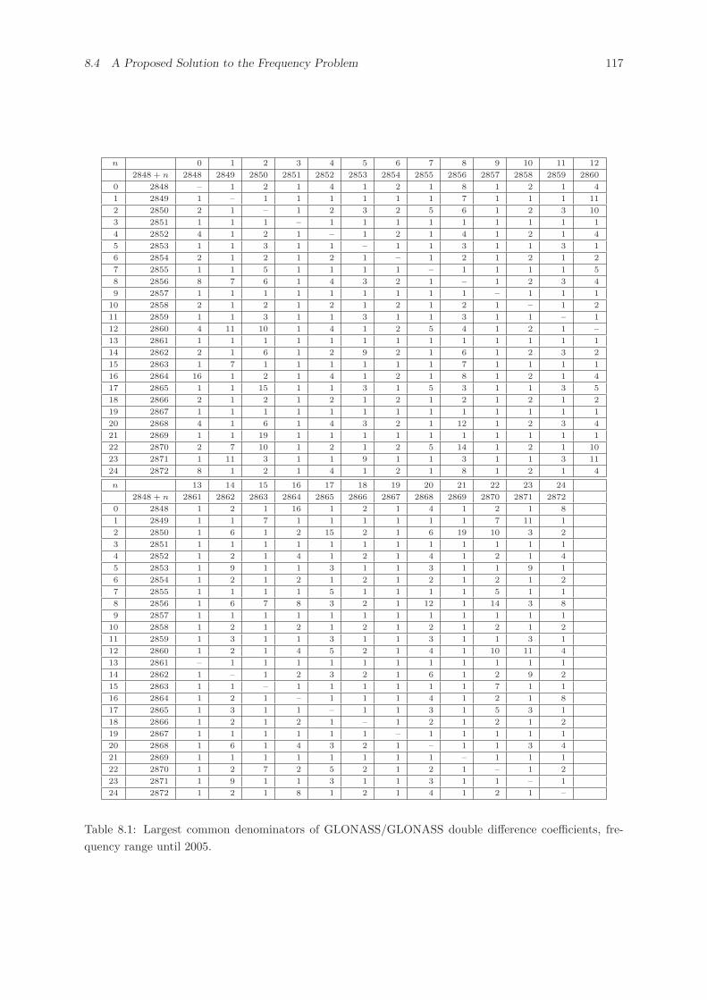
8.4 A Proposed Solution to the Frequency Problem 117
n 0 1 2 3 4 5 6 7 8 9 10 11 12
2848 + n 2848 2849 2850 2851 2852 2853 2854 2855 2856 2857 2858 2859 2860
0 2848 – 1 2 1 4 1 2 1 8 1 2 1 4
1 2849 1 – 1 1 1 1 1 1 7 1 1 1 11
2 2850 2 1 – 1 2 3 2 5 6 1 2 3 10
3 2851 1 1 1 – 1 1 1 1 1 1 1 1 1
4 2852 4 1 2 1 – 1 2 1 4 1 2 1 4
5 2853 1 1 3 1 1 – 1 1 3 1 1 3 1
6 2854 2 1 2 1 2 1 – 1 2 1 2 1 2
7 2855 1 1 5 1 1 1 1 – 1 1 1 1 5
8 2856 8 7 6 1 4 3 2 1 – 1 2 3 4
9 2857 1 1 1 1 1 1 1 1 1 – 1 1 1
10 2858 2 1 2 1 2 1 2 1 2 1 – 1 2
11 2859 1 1 3 1 1 3 1 1 3 1 1 – 1
12 2860 4 11 10 1 4 1 2 5 4 1 2 1 –
13 2861 1 1 1 1 1 1 1 1 1 1 1 1 1
14 2862 2 1 6 1 2 9 2 1 6 1 2 3 2
15 2863 1 7 1 1 1 1 1 1 7 1 1 1 1
16 2864 16 1 2 1 4 1 2 1 8 1 2 1 4
17 2865 1 1 15 1 1 3 1 5 3 1 1 3 5
18 2866 2 1 2 1 2 1 2 1 2 1 2 1 2
19 2867 1 1 1 1 1 1 1 1 1 1 1 1 1
20 2868 4 1 6 1 4 3 2 1 12 1 2 3 4
21 2869 1 1 19 1 1 1 1 1 1 1 1 1 1
22 2870 2 7 10 1 2 1 2 5 14 1 2 1 10
23 2871 1 11 3 1 1 9 1 1 3 1 1 3 11
24 2872 8 1 2 1 4 1 2 1 8 1 2 1 4
n 13 14 15 16 17 18 19 20 21 22 23 24
2848 + n 2861 2862 2863 2864 2865 2866 2867 2868 2869 2870 2871 2872
0 2848 1 2 1 16 1 2 1 4 1 2 1 8
1 2849 1 1 7 1 1 1 1 1 1 7 11 1
2 2850 1 6 1 2 15 2 1 6 19 10 3 2
3 2851 1 1 1 1 1 1 1 1 1 1 1 1
4 2852 1 2 1 4 1 2 1 4 1 2 1 4
5 2853 1 9 1 1 3 1 1 3 1 1 9 1
6 2854 1 2 1 2 1 2 1 2 1 2 1 2
7 2855 1 1 1 1 5 1 1 1 1 5 1 1
8 2856 1 6 7 8 3 2 1 12 1 14 3 8
9 2857 1 1 1 1 1 1 1 1 1 1 1 1
10 2858 1 2 1 2 1 2 1 2 1 2 1 2
11 2859 1 3 1 1 3 1 1 3 1 1 3 1
12 2860 1 2 1 4 5 2 1 4 1 10 11 4
13 2861 – 1 1 1 1 1 1 1 1 1 1 1
14 2862 1 – 1 2 3 2 1 6 1 2 9 2
15 2863 1 1 – 1 1 1 1 1 1 7 1 1
16 2864 1 2 1 – 1 1 1 4 1 2 1 8
17 2865 1 3 1 1 – 1 1 3 1 5 3 1
18 2866 1 2 1 2 1 – 1 2 1 2 1 2
19 2867 1 1 1 1 1 1 – 1 1 1 1 1
20 2868 1 6 1 4 3 2 1 – 1 1 3 4
21 2869 1 1 1 1 1 1 1 1 – 1 1 1
22 2870 1 2 7 2 5 2 1 2 1 – 1 2
23 2871 1 9 1 1 3 1 1 3 1 1 – 1
24 2872 1 2 1 8 1 2 1 4 1 2 1 –
Table 8.1: Largest common denominators of GLONASS/GLONASS double difference coefficients, fre-quency range until 2005.
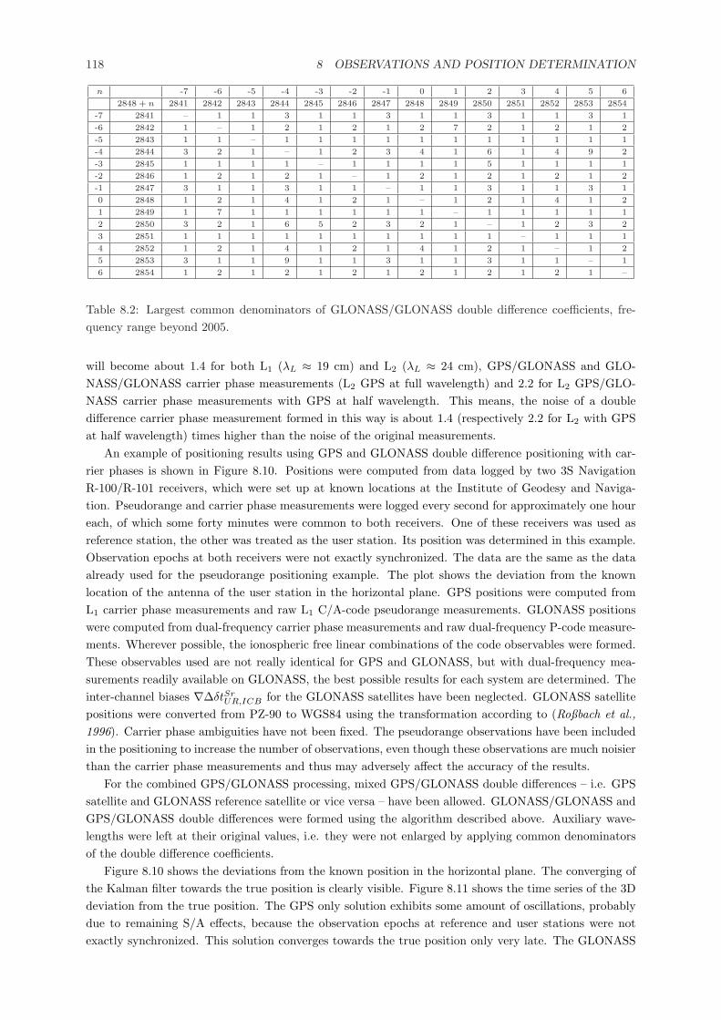
118 8 OBSERVATIONS AND POSITION DETERMINATION
n -7 -6 -5 -4 -3 -2 -1 0 1 2 3 4 5 6
2848 + n 2841 2842 2843 2844 2845 2846 2847 2848 2849 2850 2851 2852 2853 2854
-7 2841 – 1 1 3 1 1 3 1 1 3 1 1 3 1
-6 2842 1 – 1 2 1 2 1 2 7 2 1 2 1 2
-5 2843 1 1 – 1 1 1 1 1 1 1 1 1 1 1
-4 2844 3 2 1 – 1 2 3 4 1 6 1 4 9 2
-3 2845 1 1 1 1 – 1 1 1 1 5 1 1 1 1
-2 2846 1 2 1 2 1 – 1 2 1 2 1 2 1 2
-1 2847 3 1 1 3 1 1 – 1 1 3 1 1 3 1
0 2848 1 2 1 4 1 2 1 – 1 2 1 4 1 2
1 2849 1 7 1 1 1 1 1 1 – 1 1 1 1 1
2 2850 3 2 1 6 5 2 3 2 1 – 1 2 3 2
3 2851 1 1 1 1 1 1 1 1 1 1 – 1 1 1
4 2852 1 2 1 4 1 2 1 4 1 2 1 – 1 2
5 2853 3 1 1 9 1 1 3 1 1 3 1 1 – 1
6 2854 1 2 1 2 1 2 1 2 1 2 1 2 1 –
Table 8.2: Largest common denominators of GLONASS/GLONASS double difference coefficients, fre-quency range beyond 2005.
will become about 1.4 for both L1 (λL ≈ 19 cm) and L2 (λL ≈ 24 cm), GPS/GLONASS and GLO-NASS/GLONASS carrier phase measurements (L2 GPS at full wavelength) and 2.2 for L2 GPS/GLO-NASS carrier phase measurements with GPS at half wavelength. This means, the noise of a doubledifference carrier phase measurement formed in this way is about 1.4 (respectively 2.2 for L2 with GPSat half wavelength) times higher than the noise of the original measurements.
An example of positioning results using GPS and GLONASS double difference positioning with car-rier phases is shown in Figure 8.10. Positions were computed from data logged by two 3S NavigationR-100/R-101 receivers, which were set up at known locations at the Institute of Geodesy and Naviga-tion. Pseudorange and carrier phase measurements were logged every second for approximately one houreach, of which some forty minutes were common to both receivers. One of these receivers was used asreference station, the other was treated as the user station. Its position was determined in this example.Observation epochs at both receivers were not exactly synchronized. The data are the same as the dataalready used for the pseudorange positioning example. The plot shows the deviation from the knownlocation of the antenna of the user station in the horizontal plane. GPS positions were computed fromL1 carrier phase measurements and raw L1 C/A-code pseudorange measurements. GLONASS positionswere computed from dual-frequency carrier phase measurements and raw dual-frequency P-code measure-ments. Wherever possible, the ionospheric free linear combinations of the code observables were formed.These observables used are not really identical for GPS and GLONASS, but with dual-frequency mea-surements readily available on GLONASS, the best possible results for each system are determined. Theinter-channel biases ∇∆δtSr
UR,ICB for the GLONASS satellites have been neglected. GLONASS satellitepositions were converted from PZ-90 to WGS84 using the transformation according to (Roßbach et al.,1996). Carrier phase ambiguities have not been fixed. The pseudorange observations have been includedin the positioning to increase the number of observations, even though these observations are much noisierthan the carrier phase measurements and thus may adversely affect the accuracy of the results.
For the combined GPS/GLONASS processing, mixed GPS/GLONASS double differences – i.e. GPSsatellite and GLONASS reference satellite or vice versa – have been allowed. GLONASS/GLONASS andGPS/GLONASS double differences were formed using the algorithm described above. Auxiliary wave-lengths were left at their original values, i.e. they were not enlarged by applying common denominatorsof the double difference coefficients.
Figure 8.10 shows the deviations from the known position in the horizontal plane. The converging ofthe Kalman filter towards the true position is clearly visible. Figure 8.11 shows the time series of the 3Ddeviation from the true position. The GPS only solution exhibits some amount of oscillations, probablydue to remaining S/A effects, because the observation epochs at reference and user stations were notexactly synchronized. This solution converges towards the true position only very late. The GLONASS
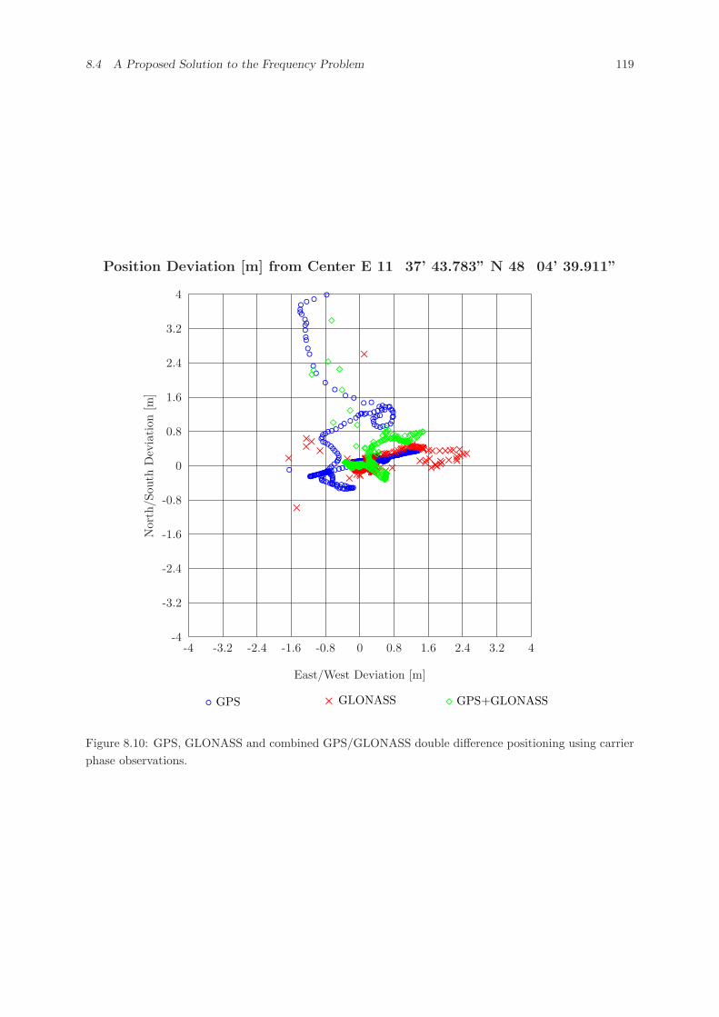
8.4 A Proposed Solution to the Frequency Problem 119
Position Deviation [m] from Center E 11� 37’ 43.783” N 48� 04’ 39.911”
◦ GPS × GLONASS ¦ GPS+GLONASS
East/West Deviation [m]
-4 -3.2 -2.4 -1.6 -0.8 0 0.8 1.6 2.4 3.2 4
Nor
th/S
outh
Dev
iati
on[m
]
-4
-3.2
-2.4
-1.6
-0.8
0
0.8
1.6
2.4
3.2
4
◦
◦◦◦◦◦◦◦◦◦◦◦◦◦◦◦◦◦ ◦ ◦ ◦◦ ◦◦◦◦◦◦◦◦◦◦◦◦◦◦◦◦◦◦◦
◦◦◦◦◦◦◦◦◦◦◦◦◦◦◦◦◦◦◦◦◦◦◦◦◦◦◦◦◦◦◦◦◦◦◦◦◦◦◦◦◦◦◦◦◦◦◦◦◦◦◦◦◦◦◦◦◦◦◦◦◦◦◦◦◦◦◦◦◦◦◦◦◦◦◦◦◦◦◦◦◦◦◦◦◦◦◦◦◦◦◦◦◦◦◦◦◦◦◦◦◦◦◦◦◦◦◦◦◦◦◦◦◦◦◦◦◦◦◦◦◦◦◦◦◦◦
◦◦◦◦◦◦◦◦◦◦◦◦◦◦◦◦◦◦◦◦◦◦◦◦◦◦◦◦◦◦◦◦◦◦◦◦◦◦◦◦◦◦◦◦◦◦◦◦◦◦◦◦◦◦◦◦◦◦◦◦◦◦◦◦◦◦◦◦◦◦◦◦◦◦◦◦◦◦◦◦◦◦◦◦◦◦◦◦◦◦◦◦◦◦◦◦◦◦◦◦◦◦◦◦◦◦◦◦◦◦◦◦◦◦◦◦◦◦◦◦◦◦◦◦◦◦◦◦◦◦◦◦◦◦◦◦◦◦◦◦◦◦◦◦◦◦◦◦◦◦◦◦◦◦◦◦◦◦◦◦◦◦◦◦◦◦◦◦◦◦◦◦◦◦◦◦◦◦◦◦◦◦◦◦◦◦◦◦◦◦◦◦◦◦◦◦◦◦◦◦◦◦◦◦◦◦◦◦◦◦◦◦◦◦◦◦◦◦◦◦◦◦◦◦◦◦◦◦◦◦◦◦◦◦◦◦◦◦◦◦◦◦◦◦◦◦◦◦◦◦◦◦◦◦◦◦◦◦◦◦◦◦◦◦◦◦◦◦◦◦◦◦◦◦◦◦◦◦◦◦◦◦◦◦◦◦◦◦◦◦◦◦◦◦◦◦◦◦◦◦◦◦◦◦◦◦◦◦◦◦◦◦◦◦◦◦◦◦◦◦◦◦◦◦◦◦◦◦◦◦◦◦◦◦◦◦◦◦◦◦◦◦◦◦◦◦◦◦◦◦◦◦◦◦◦◦◦◦◦◦◦◦◦◦◦◦◦◦◦◦◦◦◦◦◦◦◦◦◦◦◦◦◦◦◦◦◦◦◦◦◦◦◦◦◦◦◦◦◦◦◦◦◦◦◦◦◦◦◦◦◦◦◦◦◦◦◦◦◦◦◦◦◦◦◦◦◦◦◦◦◦◦◦◦◦◦◦◦◦◦◦◦◦◦◦◦◦◦◦◦◦◦◦◦◦◦◦◦◦◦◦◦◦◦◦◦◦◦◦◦◦◦◦◦◦◦◦◦◦◦◦◦◦◦◦◦◦◦◦◦◦◦◦◦◦◦◦◦◦◦◦◦◦◦◦◦◦◦◦◦◦◦◦◦◦◦◦◦◦◦◦◦◦◦◦◦◦◦◦◦◦◦◦◦◦◦◦◦◦◦◦◦◦◦◦◦◦◦◦◦◦◦◦◦◦◦◦◦◦◦◦◦◦◦◦◦◦◦◦◦◦◦◦◦◦◦◦◦◦◦◦◦◦◦◦◦◦◦◦◦◦◦◦◦◦◦◦◦◦◦◦◦◦◦◦◦◦◦◦◦◦◦◦◦◦◦◦◦◦◦◦◦◦◦◦◦◦◦◦◦◦◦◦◦◦◦◦◦◦◦◦◦◦◦◦◦◦◦◦◦◦◦◦◦◦◦◦◦◦◦◦◦◦◦◦◦◦◦◦◦◦◦◦◦◦◦◦◦◦◦◦◦◦◦◦◦◦◦◦◦◦◦◦◦◦◦◦◦◦◦◦◦◦◦◦◦◦◦◦◦◦◦◦◦◦◦◦◦◦◦◦◦◦◦◦◦◦◦◦◦◦◦◦◦◦◦◦◦◦◦◦◦◦◦◦◦◦◦◦◦◦◦◦◦◦◦◦◦◦◦◦◦◦◦◦◦◦◦◦◦◦◦◦◦◦◦◦◦◦◦◦◦◦◦◦◦◦◦◦◦◦◦◦◦◦◦◦◦◦◦◦◦◦◦◦◦◦◦◦◦◦◦◦◦◦◦◦◦◦◦◦◦◦◦◦◦◦◦◦◦◦◦◦◦◦◦◦◦◦◦◦◦◦◦◦◦◦◦◦◦◦◦◦◦◦◦◦◦◦◦◦◦◦◦◦◦◦◦◦◦◦◦◦◦◦◦◦◦◦◦◦◦◦◦◦◦◦◦◦◦◦◦◦◦◦◦◦◦◦◦◦◦◦◦◦◦◦◦◦◦◦◦◦◦◦◦◦◦◦◦◦◦◦◦◦◦◦◦◦◦◦◦◦◦◦◦◦◦◦◦◦◦◦◦◦◦◦◦◦◦◦◦◦◦◦◦◦◦◦◦◦◦◦◦◦◦◦◦◦◦◦◦◦◦◦◦◦◦◦◦◦◦◦◦◦◦◦◦◦◦◦◦◦◦◦◦◦◦◦◦◦◦◦◦◦◦◦◦◦◦◦◦◦◦◦◦◦◦◦◦◦◦◦◦◦◦◦◦◦◦◦◦◦◦◦◦◦◦◦◦◦◦◦◦◦◦◦◦◦◦◦◦◦◦◦◦◦◦◦◦◦◦◦◦◦◦◦◦◦◦◦◦◦◦◦◦◦◦◦◦◦◦◦◦◦◦◦◦◦◦◦◦◦◦◦◦◦◦◦◦◦◦◦◦◦◦◦◦◦◦◦◦◦◦◦◦◦◦◦◦◦◦◦◦◦◦◦◦◦◦◦◦◦◦◦◦◦◦◦◦◦◦◦◦◦◦◦◦◦◦◦◦◦◦◦◦◦◦◦◦◦◦◦◦◦◦◦◦◦◦◦◦◦◦◦◦◦◦◦◦◦◦◦◦◦◦◦◦◦◦◦◦◦◦◦◦◦◦◦◦◦◦◦◦◦◦◦◦◦◦◦◦◦◦◦◦◦◦◦◦◦◦◦◦◦◦◦◦◦◦◦◦◦◦◦◦◦◦◦◦◦◦◦◦◦◦◦◦◦◦◦◦◦◦◦◦◦◦◦◦◦◦◦◦◦◦◦◦◦◦◦◦◦◦◦◦◦◦◦◦◦◦◦◦◦◦◦◦◦◦◦◦◦◦◦◦◦◦◦◦◦◦◦◦◦◦◦◦◦◦◦◦◦◦◦◦◦◦◦◦◦◦◦◦◦◦◦◦◦◦◦◦◦◦◦◦◦◦◦◦◦◦◦◦◦◦◦◦◦◦◦◦◦◦◦◦◦◦◦◦◦◦◦◦◦◦◦◦◦◦◦◦◦◦◦◦◦◦◦◦◦◦◦◦◦◦◦◦◦◦◦◦◦◦◦◦◦◦◦◦◦◦◦◦◦◦◦◦◦◦◦◦◦◦◦◦◦◦◦◦◦◦◦◦◦◦◦◦◦◦◦◦◦◦◦◦◦◦◦◦◦◦◦◦◦◦◦◦◦◦◦◦◦◦◦◦◦◦◦◦◦◦◦◦◦◦◦◦◦◦◦◦
×
×××
× ×
×
××××××××××× ×××××××××××××××××××××××××××××××××××××××××××××××××××××××××××××××××××××××××××××××××××××××××××××××××××××××××××××××××××××××××××××××××××××××××××××××××××××××××××××××××××××××××××××××××××××××××××××××××××××××××××××××××××××××××××××××××××××××××××××××××××××××××××××××××××××××××××××××××××××××××××××××××××××××××××××××××××××××××××××××××××××××××××××××××××××××××××××××××××××××××××××××××××××××××××××××××××××××××××××××××××××××××××××××××××××××××××××××××××××××××××××××××××××××××××××××××××××××××××××××××××××××××××××××××××××××××××××××××××××××××××××××××××××××××××××××××××××××××××××××××××××××××××××××××××××××××××××××××××××××××××××××××××××××××××××××××××××××××××××××××××××××××××××××××××××××××××××××××××××××××××××××××××××××××××××××××××××××××××××××××××××××××××××××××××××××××××××××××××××××××××××××××××××××××××××××××××××××××××××××××××××××××××××××××××××××××××××××××××××××××××××××××××××××××××××××××××××××××××××××××××××××××××××××××××××××××××××××××××××××××××××××××××××××××××××××××××××××××××××××××××××××××××××××××××××××××××××××××××××××××××××××××××××××××××××××××××××××××××××××××××××××××××××××××××××××××××××××××××××××××××××××××××××××××××××××××××××××××××××××××××××××××××××××××××××××××××××××××××××××××××××××××××××××××××××××××××××××××××××××××××××
¦
¦¦¦¦
¦
¦¦¦¦¦¦¦¦¦¦¦¦
¦¦¦¦¦¦¦¦¦¦¦¦¦¦¦¦¦¦¦¦¦¦¦¦¦¦¦¦¦¦¦¦¦¦¦¦¦¦¦¦¦¦¦¦¦¦¦¦¦¦¦¦¦¦¦¦¦¦¦¦¦¦¦¦¦¦¦¦¦¦¦¦¦¦¦¦¦¦¦¦¦¦¦¦¦¦¦¦¦¦¦¦¦¦¦¦¦¦¦¦¦¦¦¦¦¦¦¦¦¦¦¦¦¦¦¦¦¦¦¦¦¦¦¦¦¦¦¦¦¦¦¦¦¦¦¦¦¦¦¦¦¦¦¦¦¦¦¦¦¦¦¦¦¦¦¦¦¦¦¦¦¦¦¦¦¦¦¦¦¦¦¦¦¦¦¦¦¦¦¦¦¦¦¦¦¦¦¦¦¦¦¦¦¦¦¦¦¦¦¦¦¦¦¦¦¦¦¦¦¦¦¦¦¦¦¦¦¦¦¦¦¦¦¦¦¦¦¦¦¦¦¦¦¦¦¦¦¦¦¦¦¦¦¦¦¦¦¦¦¦¦¦¦¦¦¦¦¦¦¦¦¦¦¦¦¦¦¦¦¦¦¦¦¦¦¦¦¦¦¦¦¦¦¦¦¦¦¦¦¦¦¦¦¦¦¦¦¦¦¦¦¦¦¦¦¦¦¦¦¦¦¦¦¦¦¦¦¦¦¦¦¦¦¦¦¦¦¦¦¦¦¦¦¦¦¦¦¦¦¦¦¦¦¦¦¦¦¦¦¦¦¦¦¦¦¦¦¦¦¦¦¦¦¦¦¦¦¦¦¦¦¦¦¦¦¦¦¦¦¦¦¦¦¦¦¦¦¦¦¦¦¦¦¦¦¦¦¦¦¦¦¦¦¦¦¦¦¦¦¦¦¦¦¦¦¦¦¦¦¦¦¦¦¦¦¦¦¦¦¦¦¦¦¦¦¦¦¦¦¦¦¦¦¦¦¦¦¦¦¦¦¦¦¦¦¦¦¦¦¦¦¦¦¦¦¦¦¦¦¦¦¦¦¦¦¦¦¦¦¦¦¦¦¦¦¦¦¦¦¦¦¦¦¦¦¦¦¦¦¦¦¦¦¦¦¦¦¦¦¦¦¦¦¦¦¦¦¦¦¦¦¦¦¦¦¦¦¦¦¦¦¦¦¦¦¦¦¦¦¦¦¦¦¦¦¦¦¦¦¦¦¦¦¦¦¦¦¦¦¦¦¦¦¦¦¦¦¦¦¦¦¦¦¦¦¦¦¦¦¦¦¦¦¦¦¦¦¦¦¦¦¦¦¦¦¦¦¦¦¦¦¦¦¦¦¦¦¦¦¦¦¦¦¦¦¦¦¦¦¦¦¦¦¦¦¦¦¦¦¦¦¦¦¦¦¦¦¦¦¦¦¦¦¦¦¦¦¦¦¦¦¦¦¦¦¦¦¦¦¦¦¦¦¦¦¦¦¦¦¦¦¦¦¦¦¦¦¦¦¦¦¦¦¦¦¦¦¦¦¦¦¦¦¦¦¦¦¦¦¦¦¦¦¦¦¦¦¦¦¦¦¦¦¦¦¦¦¦¦¦¦¦¦¦¦¦¦¦¦¦¦¦¦¦¦¦¦¦¦¦¦¦¦¦¦¦¦¦¦¦¦¦¦¦¦¦¦¦¦¦¦¦¦¦¦¦¦¦¦¦¦¦¦¦¦¦¦¦¦¦¦¦¦¦¦¦¦¦¦¦¦¦¦¦¦¦¦¦¦¦¦¦¦¦¦¦¦¦¦¦¦¦¦¦¦¦¦¦¦¦¦¦¦¦¦¦¦¦¦¦¦¦¦¦¦¦¦¦¦¦¦¦¦¦¦¦¦¦¦¦¦¦¦¦¦¦¦¦¦¦¦¦¦¦¦¦¦¦¦¦¦¦¦¦¦¦¦¦¦¦¦¦¦¦¦¦¦¦¦¦¦¦¦¦¦¦¦¦¦¦¦¦¦¦¦¦¦¦¦¦¦¦¦¦¦¦¦¦¦¦¦¦¦¦¦¦¦¦¦
Figure 8.10: GPS, GLONASS and combined GPS/GLONASS double difference positioning using carrierphase observations.
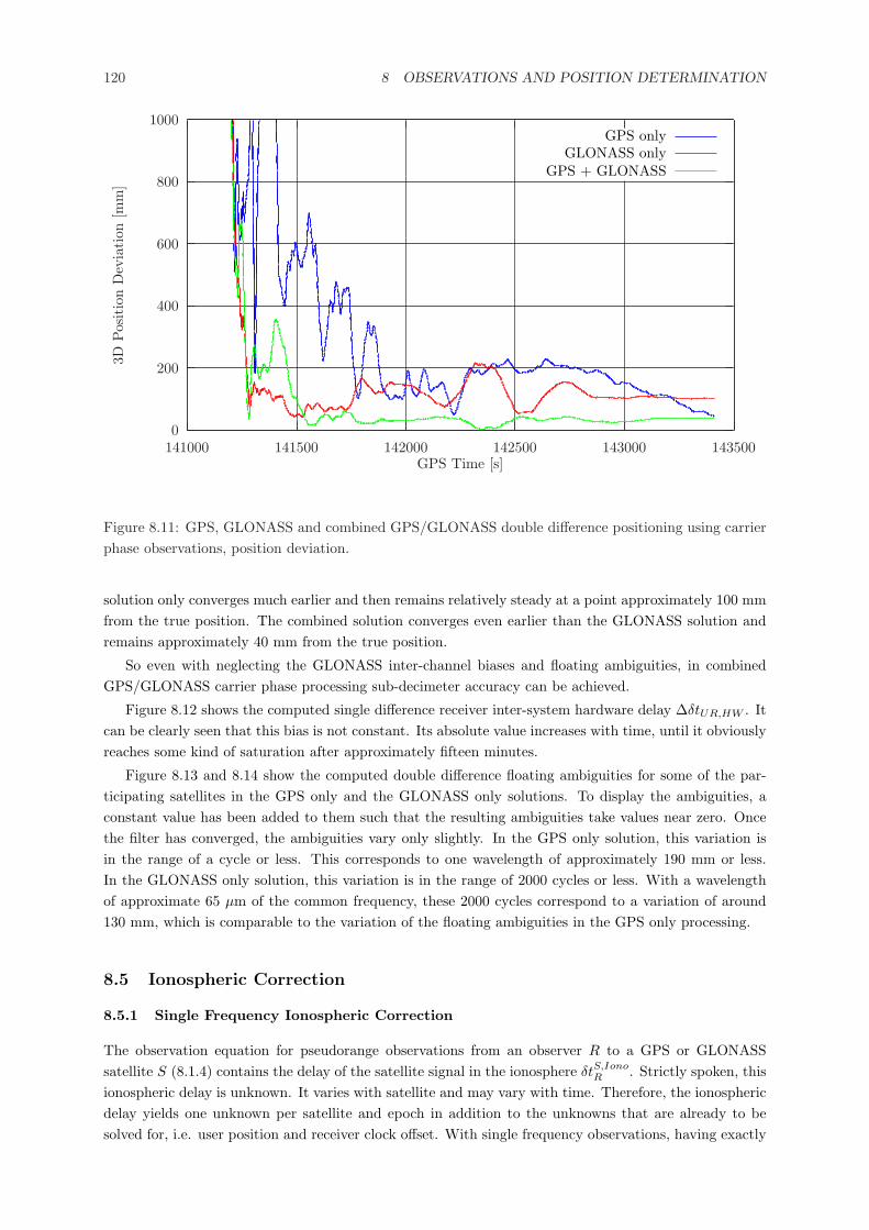
120 8 OBSERVATIONS AND POSITION DETERMINATION
0
200
400
600
800
1000
141000 141500 142000 142500 143000 143500
3DPos
itio
nD
evia
tion
[mm
]
GPS Time [s]
GPS onlyGLONASS only
GPS + GLONASS
Figure 8.11: GPS, GLONASS and combined GPS/GLONASS double difference positioning using carrierphase observations, position deviation.
solution only converges much earlier and then remains relatively steady at a point approximately 100 mmfrom the true position. The combined solution converges even earlier than the GLONASS solution andremains approximately 40 mm from the true position.
So even with neglecting the GLONASS inter-channel biases and floating ambiguities, in combinedGPS/GLONASS carrier phase processing sub-decimeter accuracy can be achieved.
Figure 8.12 shows the computed single difference receiver inter-system hardware delay ∆δtUR,HW . Itcan be clearly seen that this bias is not constant. Its absolute value increases with time, until it obviouslyreaches some kind of saturation after approximately fifteen minutes.
Figure 8.13 and 8.14 show the computed double difference floating ambiguities for some of the par-ticipating satellites in the GPS only and the GLONASS only solutions. To display the ambiguities, aconstant value has been added to them such that the resulting ambiguities take values near zero. Oncethe filter has converged, the ambiguities vary only slightly. In the GPS only solution, this variation isin the range of a cycle or less. This corresponds to one wavelength of approximately 190 mm or less.In the GLONASS only solution, this variation is in the range of 2000 cycles or less. With a wavelengthof approximate 65 µm of the common frequency, these 2000 cycles correspond to a variation of around130 mm, which is comparable to the variation of the floating ambiguities in the GPS only processing.
8.5 Ionospheric Correction
8.5.1 Single Frequency Ionospheric Correction
The observation equation for pseudorange observations from an observer R to a GPS or GLONASSsatellite S (8.1.4) contains the delay of the satellite signal in the ionosphere δtS,Iono
R . Strictly spoken, thisionospheric delay is unknown. It varies with satellite and may vary with time. Therefore, the ionosphericdelay yields one unknown per satellite and epoch in addition to the unknowns that are already to besolved for, i.e. user position and receiver clock offset. With single frequency observations, having exactly
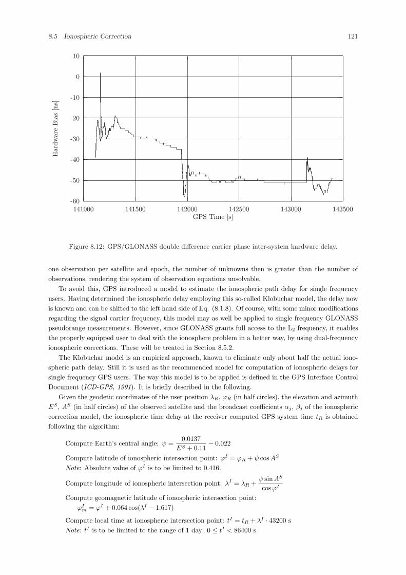
8.5 Ionospheric Correction 121
-60
-50
-40
-30
-20
-10
0
10
141000 141500 142000 142500 143000 143500
Har
dwar
eB
ias
[ns]
GPS Time [s]
Figure 8.12: GPS/GLONASS double difference carrier phase inter-system hardware delay.
one observation per satellite and epoch, the number of unknowns then is greater than the number ofobservations, rendering the system of observation equations unsolvable.
To avoid this, GPS introduced a model to estimate the ionospheric path delay for single frequencyusers. Having determined the ionospheric delay employing this so-called Klobuchar model, the delay nowis known and can be shifted to the left hand side of Eq. (8.1.8). Of course, with some minor modificationsregarding the signal carrier frequency, this model may as well be applied to single frequency GLONASSpseudorange measurements. However, since GLONASS grants full access to the L2 frequency, it enablesthe properly equipped user to deal with the ionosphere problem in a better way, by using dual-frequencyionospheric corrections. These will be treated in Section 8.5.2.
The Klobuchar model is an empirical approach, known to eliminate only about half the actual iono-spheric path delay. Still it is used as the recommended model for computation of ionospheric delays forsingle frequency GPS users. The way this model is to be applied is defined in the GPS Interface ControlDocument (ICD-GPS, 1991). It is briefly described in the following.
Given the geodetic coordinates of the user position λR, ϕR (in half circles), the elevation and azimuthES , AS (in half circles) of the observed satellite and the broadcast coefficients αj , βj of the ionosphericcorrection model, the ionospheric time delay at the receiver computed GPS system time tR is obtainedfollowing the algorithm:
Compute Earth’s central angle: ψ =0.0137
ES + 0.11− 0.022
Compute latitude of ionospheric intersection point: ϕI = ϕR + ψ cosAS
Note: Absolute value of ϕI is to be limited to 0.416.
Compute longitude of ionospheric intersection point: λI = λR +ψ sin AS
cos ϕI
Compute geomagnetic latitude of ionospheric intersection point:ϕI
m = ϕI + 0.064 cos(λI − 1.617)
Compute local time at ionospheric intersection point: tI = tR + λI · 43200 sNote: tI is to be limited to the range of 1 day: 0 ≤ tI < 86400 s.
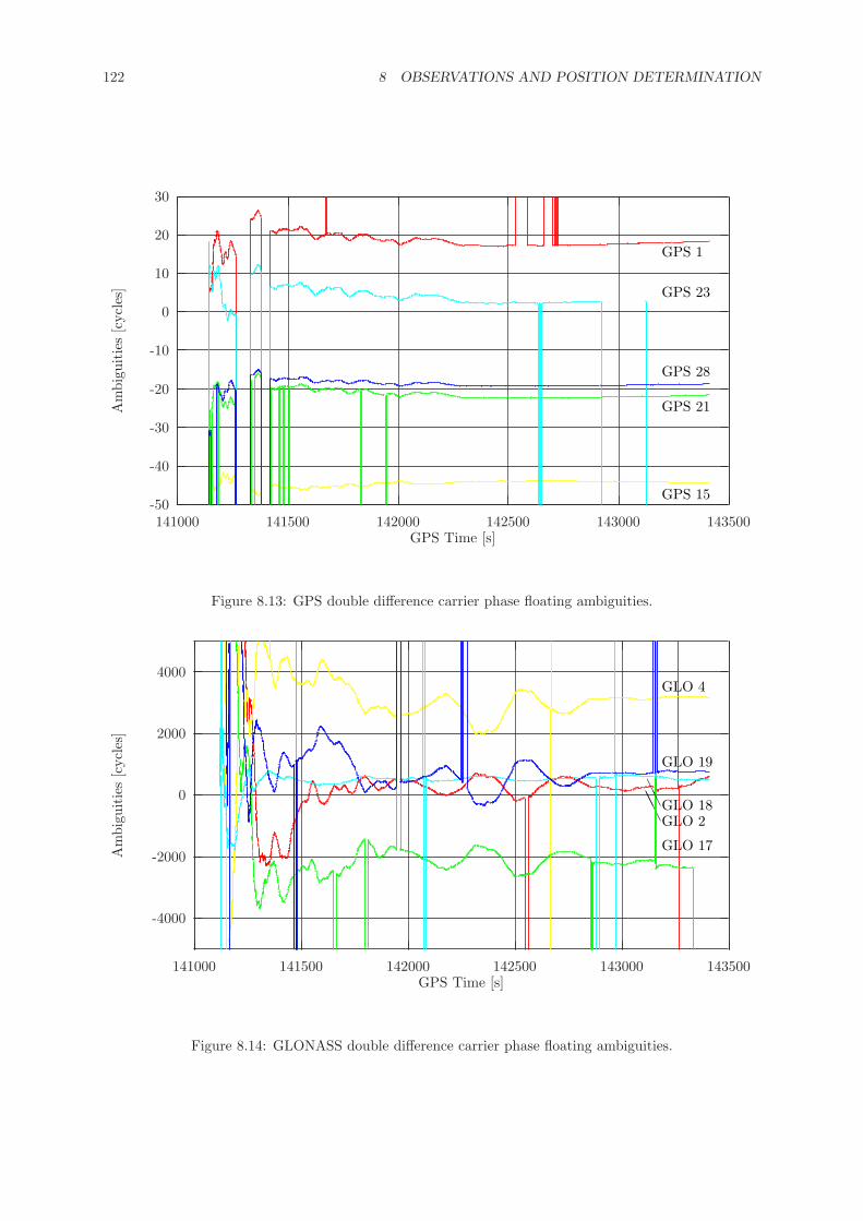
122 8 OBSERVATIONS AND POSITION DETERMINATION
-50
-40
-30
-20
-10
0
10
20
30
141000 141500 142000 142500 143000 143500
Am
bigu
itie
s[c
ycle
s]
GPS Time [s]
GPS 1
GPS 15
GPS 21
GPS 23
GPS 28
Figure 8.13: GPS double difference carrier phase floating ambiguities.
-4000
-2000
0
2000
4000
141000 141500 142000 142500 143000 143500
Am
bigu
itie
s[c
ycle
s]
GPS Time [s]
GLO 2AAA
GLO 4
GLO 17
GLO 18AA
GLO 19
Figure 8.14: GLONASS double difference carrier phase floating ambiguities.
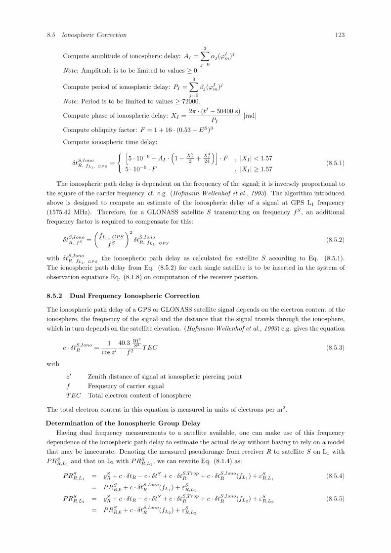
8.5 Ionospheric Correction 123
Compute amplitude of ionospheric delay: AI =3∑
j=0
αj(ϕIm)j
Note: Amplitude is to be limited to values ≥ 0.
Compute period of ionospheric delay: PI =3∑
j=0
βj(ϕIm)j
Note: Period is to be limited to values ≥ 72000.
Compute phase of ionospheric delay: XI =2π · (tI − 50400 s)
PI[rad]
Compute obliquity factor: F = 1 + 16 · (0.53− ES)3
Compute ionospheric time delay:
δtS,IonoR, fL1, GP S
=
{ [5 · 10−9 + AI ·
(1− X2
I
2 + X4I
24
)]· F , |XI | < 1.57
5 · 10−9 · F , |XI | ≥ 1.57(8.5.1)
The ionospheric path delay is dependent on the frequency of the signal; it is inversely proportional tothe square of the carrier frequency, cf. e.g. (Hofmann-Wellenhof et al., 1993). The algorithm introducedabove is designed to compute an estimate of the ionospheric delay of a signal at GPS L1 frequency(1575.42 MHz). Therefore, for a GLONASS satellite S transmitting on frequency fS , an additionalfrequency factor is required to compensate for this:
δtS,IonoR, fS =
(fL1, GPS
fS
)2
δtS,IonoR, fL1, GP S
(8.5.2)
with δtS,IonoR, fL1, GP S
the ionospheric path delay as calculated for satellite S according to Eq. (8.5.1).The ionospheric path delay from Eq. (8.5.2) for each single satellite is to be inserted in the system ofobservation equations Eq. (8.1.8) on computation of the receiver position.
8.5.2 Dual Frequency Ionospheric Correction
The ionospheric path delay of a GPS or GLONASS satellite signal depends on the electron content of theionosphere, the frequency of the signal and the distance that the signal travels through the ionosphere,which in turn depends on the satellite elevation. (Hofmann-Wellenhof et al., 1993) e.g. gives the equation
c · δtS,IonoR =
1cos z′
40.3 m3
s2
f2TEC (8.5.3)
with
z′ Zenith distance of signal at ionospheric piercing pointf Frequency of carrier signalTEC Total electron content of ionosphere
The total electron content in this equation is measured in units of electrons per m2.
Determination of the Ionospheric Group DelayHaving dual frequency measurements to a satellite available, one can make use of this frequency
dependence of the ionospheric path delay to estimate the actual delay without having to rely on a modelthat may be inaccurate. Denoting the measured pseudorange from receiver R to satellite S on L1 withPRS
R,L1and that on L2 with PRS
R,L2, we can rewrite Eq. (8.1.4) as:
PRSR,L1
= %SR + c · δtR − c · δtS + c · δtS,Trop
R + c · δtS,IonoR (fL1) + εS
R,L1(8.5.4)
= PRSR,0 + c · δtS,Iono
R (fL1) + εSR,L1
PRSR,L2
= %SR + c · δtR − c · δtS + c · δtS,Trop
R + c · δtS,IonoR (fL2) + εS
R,L2(8.5.5)
= PRSR,0 + c · δtS,Iono
R (fL2) + εSR,L2
124 8 OBSERVATIONS AND POSITION DETERMINATION
where the frequency independent parts of the pseudorange are summarized in PRSR,0. Differencing these
two measurements yields
PRSR,L2
− PRSR,L1
= c · δtS,IonoR (fL2)− c · δtS,Iono
R (fL1) + εSR,L2
− εSR,L1
(8.5.6)
By inserting Eq. (8.5.3) we obtain
PRSR,L2
− PRSR,L1
=1
cos z′40.3
m3
s2· TEC ·
(1
f2L2
− 1f2
L1
)+ εS
R,L2− εS
R,L1
=1
cos z′40.3
m3
s2· TEC · 1
f2L1
· (γ − 1) + εSR,L2
− εSR,L1
= c · δtS,IonoR (fL1) · (γ − 1) + εS
R,L2− εS
R,L1(8.5.7)
= c · δtS,IonoR (fL2) ·
γ − 1γ
+ εSR,L2
− εSR,L1
(8.5.8)
with the squared frequency ratio γ = (fL1/fL2)2. Inserting the actual value of γ = 81/49 for GLONASS
and neglecting the measurement noise, the ionospheric path delays become
c · δtS,IonoR (fL1) =
4932
(PRSR,L2
− PRSR,L1
) (8.5.9)
c · δtS,IonoR (fL2) =
8132
(PRSR,L2
− PRSR,L1
) (8.5.10)
for the pseudorange measurements on L1 and L2, respectively. These ionospheric delays for each satelliteand one measurement is to be inserted in the system of observation equations Eq. (8.1.8) on computationof the receiver position. The second measurement to that satellite now is to be discarded, because it isno longer linearly independent.
Ionospheric Free PseudorangeA different way of making use of the frequency dependence of the ionospheric path delay to elimi-
nate the influence of the ionosphere in position computation is the forming of an ionospheric-free linearcombination of the measured L1 and L2 pseudoranges.
Given two pseudorange measurements on L1 and L2 from receiver R to satellite S
PRSR,L1
= PRSR,0 + c · δtS,Iono
R (fL1) + εSR,L1
(8.5.11)
PRSR,L2
= PRSR,0 + c · δtS,Iono
R (fL2) + εSR,L2
(8.5.12)
where the frequency independent parts of the pseudorange are summarized in PRSR,0 (cf. Eq. (8.5.6)), a
linear combination can be formed by
PRSR,IF = k1 · PRS
R,L1+ k2 · PRS
R,L2(8.5.13)
where k1 and k2 are arbitrary factors to be determined in such a way that PRSR,IF does no longer contain
any influence of the ionosphere. Measurement noise again is neglected. However, such a combinationis likely to result in an ionospheric free pseudorange that is no longer in the order of magnitude of themeasured pseudoranges (including all clock and other errors). When trying to compute a positioningsolution from e.g. Eq. (8.1.8) with these ”measured” values, one may obtain unlikely large residuals andtherewith inaccurate positions. To avoid this, the linear combination from Eq. (8.5.13) is scaled back tothe order of magnitude of the measured pseudoranges. This is accomplished by ensuring that the sum ofthe linear factors is equal to 1:
PRSR,IF =
k1
k1 + k2· PRS
R,L1+
k2
k1 + k2· PRS
R,L2(8.5.14)
To match the condition that the ionospheric free pseudorange no longer contain any influence of theionosphere, it is necessary that the linear combination of the ionospheric delays on both measurementsdisappears:
k1 · c · δtS,IonoR (fL1) + k2 · c · δtS,Iono
R (fL2)!= 0 (8.5.15)
8.5 Ionospheric Correction 125
Eq. (8.5.15) contains two unknowns, k1 and k2. Therefore, one unknown may be chosen arbitrarilyto enable solution of the equation. Choosing k1 = 1, we obtain
k2 = −c · δtS,IonoR (fL1)
c · δtS,IonoR (fL2)
(8.5.16)
and by inserting Eq. (8.5.3)
k2 = − 1γ
(8.5.17)
Inserting these factors k1 and k2 into Eq. (8.5.14) yields the ionospheric free pseudorange
PRSR,IF =
γ
γ − 1
(PRS
R,L1− 1
γPRS
R,L2
)(8.5.18)
Using this ionospheric free pseudorange from observer R to satellite S in the positioning solution, e.g.according to Eq. (8.1.8), the ionospheric path delay c · δtS,Iono
R is equal to zero.However, the noise of the ionospheric free pseudorange is increased with respect to the original pseudo-
range measurements. Applying the laws of error propagation, one obtains for the noise of the ionosphericfree pseudorange:
σ2PRIF
=(
γ
γ − 1
)2
σ2PRL1
+(
1γ − 1
)2
σ2PRL2
(8.5.19)
Assuming the noise of the original pseudorange measurements on L1 and L2 to be equal, σPRL1=
σPRL2= σPR, this yields
σ2PRIF
=γ2 + 1
(γ − 1)2· σ2
PR (8.5.20)
or
σPRIF=
√γ2 + 1γ − 1
· σPR (8.5.21)
With the actual value of γ = 81/49, this becomes σPRIF ≈ 2.96 · σPR.
Ionospheric Free Carrier PhasesAnalogously to the pseudoranges, an ionospheric free linear combination of carrier phase measurements
can be formed, too. Starting from the observation equation for carrier phase measurements scaled incycles Eq. (8.2.1), analogously to Eq. (8.5.14), the ionospheric free linear combination of carrier phasemeasurements can then be written as
ϕSR,IF =
k1
k1 + k2· ϕS
R,L1+
k2
k1 + k2· ϕS
R,L2(8.5.22)
Again postulating that the ionospheric influence on this linear combination disappear:
k1 · fL1 · δtS,IonoR (fL1) + k2 · fL2 · δtS,Iono
R (fL2)!= 0 (8.5.23)
Choosing k1 = 1, we obtain for k2:
k2 = −fL1
fL2
· δtS,IonoR (fL1)
δtS,IonoR (fL2)
(8.5.24)
and by inserting Eq. (8.5.3)
k2 = − 1√γ
(8.5.25)
With these factors, the ionospheric free linear combination of carrier phase measurements becomes
ϕSR,IF =
√γ√
γ − 1
(ϕS
R,L1− 1√
γϕS
R,L2
)(8.5.26)
126 8 OBSERVATIONS AND POSITION DETERMINATION
Under the assumption of the measurement noise of the L1 carrier phase being identical to that of theL2 carrier phase, σϕL1
= σϕL2= σϕ the noise of the ionospheric free carrier phase measurement becomes
σϕIF =√
γ + 1√γ − 1
· σϕ (8.5.27)
Inserting the actual value of γ = (9/7)2, the noise of the ionospheric free carrier phase measurement isσϕIF
= 5.7 · σϕ.The wavelength of the ionospheric free carrier signal can be determined by means of the relation
λIF =c
k1fL1 + k2fL2
=c
fL1 − 1√γ fL2
=c
fL1
11− 1
γ
= λL1
γ
γ − 1(8.5.28)
With the actual value of γ = 81/49, the wavelength of the ionospheric free carrier signal becomes 2.53125times the wavelength of the L1 signal. For a GLONASS satellite using frequency number 1 with an L1
wavelength of approximately 18.707 cm, the wavelength of the ionospheric free signal is approximately47.35 cm; for frequency number 24 with circa 18.557 cm wavelength on L1, it is about 46.97 cm. Futurefrequency number -7 will provide an L1wavelength of approximately 18.76 cm and thus λIF will becomeabout 47.49 cm.
The factor k2 = −1/√
γ = −7/9 is a non-integer value. Therefore, the ionospheric free linear combina-tion of the integer ambiguities NS
R,IF = NSR,L1
− (fL2/fL1) ·NSR,L2
is no longer an integer value. To retainthe integer nature of this value, sometimes the so-called L0 combination ϕS
L0= 9 · ϕS
R,L1− 7 · ϕS
R,L2
is suggested as the ionospheric free linear combination. However, the noise of this combination isσϕL0
=√
92 + 72 · σϕ ≈ 11.4 · σϕ and thus double the value of σϕIF . The wavelength of this combi-nation is
λL0 = λL1 ·1
9− 7 1√γ
(8.5.29)
or with√
γ = 9/7
λL0 = λL1 ·9
92 − 72= 0.28125 · λL1 (8.5.30)
This is about 5.26 cm for GLONASS frequency number 1.GPS with γ = (77/60)2 provides an ionospheric free linear combination of the carrier phase mea-
surements with σϕIF = 5.74 · σϕ and a wavelength of λIF = 2.546 · λL1 or approximately 48.44 cm.While these values are comparable to GLONASS, the noise of the combination ϕL0 for GPS becomesσϕL0
=√
772 + 602 · σϕ ≈ 97.6 · σϕ at a wavelength of λL0 = 0.033 · λL1 , which corresponds to approxi-mately 0.6 cm.
High noise and small wavelength have precluded this combination from having any significant impor-tance for GPS carrier phase positioning. For GLONASS, however, these values are much more favorable.They are still not perfect, but using a low-noise GLONASS receiver one could imagine the L0 combinationgaining importance for carrier phase positioning. Today’s GLONASS receivers provide a noise level forcarrier phase measurements around 0.5 – 1 mm (1σ). For the L0 combination, this would mean a noiselevel of 0.57 – 1.14 cm, well below the 5.26 cm wavelength of the L0 signal.
8.6 Dilution of Precision
Regarding a set of observations to satellites of one system (either GPS or GLONASS) in matrix notation
~l = A · ~x + ~ε (8.6.1)
(cf. Eq. (8.1.19)), this equation can be solved according to the scheme
~x =(AT PA
)−1AT P ·~l (8.6.2)
8.6 Dilution of Precision 127
with a weight matrix P assigning weights to the individual observations, depending on quality of mea-surement, elevation angle of satellite, or whatever one chooses.
Setting the weight matrix as identity matrix P = I, i.e. weighting all satellites equally, we obtain thecofactor matrix
QX =(AT A
)−1(8.6.3)
which depends only on the geometry of the observed satellites relative to the user.For a set of n observations, the design matrix A reads
A =
x0 − x1
%10
y0 − y1
%10
z0 − z1
%10
1
x0 − x2
%20
y0 − y2
%20
z0 − z2
%20
1
......
......
x0 − xn
%n0
y0 − yn
%n0
z0 − zn
%n0
1
=
a11 a12 a13 a14
a21 a22 a23 a24
......
......
an1 an2 an3 an4
(8.6.4)
cf. Eq. (8.1.11).Thus, the cofactor matrix becomes
QX =
n∑
i=1
a2i1
n∑
i=1
ai1ai2
n∑
i=1
ai1ai3
n∑
i=1
ai1ai4
n∑
i=1
ai2ai1
n∑
i=1
a2i2
n∑
i=1
ai2ai3
n∑
i=1
ai2ai4
n∑
i=1
ai3ai1
n∑
i=1
ai3ai2
n∑
i=1
a2i3
n∑
i=1
ai3ai4
n∑
i=1
ai4ai1
n∑
i=1
ai4ai2
n∑
i=1
ai4ai3
n∑
i=1
a2i4
−1
(8.6.5)
which often is denoted as
QX =
qXX qXY qXZ qXt
qXY qY Y qY Z qY t
qXZ qY Z qZZ qZt
qXt qY t qZt qtt
(8.6.6)
The indices in this symmetric matrix depict the origin of the terms by row and column in the designmatrix, compare e.g. (Hofmann-Wellenhof et al., 1993). It can be shown that the square root of the traceof the cofactor matrix
√qXX + qY Y + qZZ + qtt is proportional to the reciprocal value of the volume of a
geometric body formed by the intersection points of the site-satellite vectors with the unit sphere centeredat the observing site (Milliken and Zoller, 1996). The volume of this body is a direct measure of thesatellite geometry at the observer. The larger this volume, the better the geometry. And the better thegeometry, the more precise the solution for point position and clock offset of the observer. The squareroot of the trace of the cofactor matrix therefore is called the geometric dilution of precision (GDOP).It is a direct measure of the precision of the combined position and timing solution. Neglecting all errorsources other than the influence of satellite geometry, the accuracy of the obtained position and timesolution will be the product of the measurement accuracy (standard deviation) σ0 and the DOP value.The smaller the DOP value, the better the positioning solution.
The GDOP can be split into two further DOPs, representing the satellite geometry with respectto the position and timing solutions separately. These are the position dilution of precision PDOP =√
qXX + qY Y + qZZ and the time dilution of precision TDOP =√
qtt. The PDOP is a measure of howprecisely the observer can compute his own position in three-dimensional space given the current satellitegeometry. Analogously, the TDOP is a measure of how precisely the observer can compute his ownreceiver clock offset with respect to system time given the current satellite geometry.
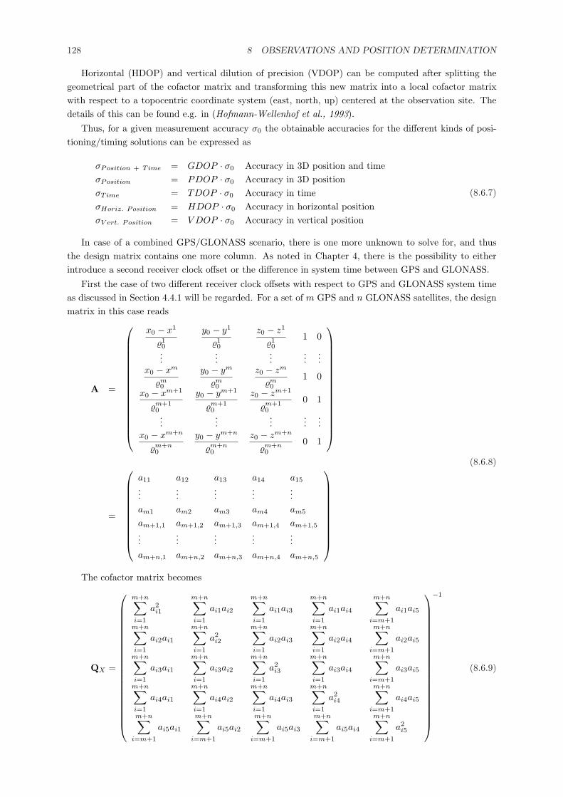
128 8 OBSERVATIONS AND POSITION DETERMINATION
Horizontal (HDOP) and vertical dilution of precision (VDOP) can be computed after splitting thegeometrical part of the cofactor matrix and transforming this new matrix into a local cofactor matrixwith respect to a topocentric coordinate system (east, north, up) centered at the observation site. Thedetails of this can be found e.g. in (Hofmann-Wellenhof et al., 1993).
Thus, for a given measurement accuracy σ0 the obtainable accuracies for the different kinds of posi-tioning/timing solutions can be expressed as
σPosition + Time = GDOP · σ0 Accuracy in 3D position and timeσPosition = PDOP · σ0 Accuracy in 3D positionσTime = TDOP · σ0 Accuracy in timeσHoriz. Position = HDOP · σ0 Accuracy in horizontal positionσV ert. Position = V DOP · σ0 Accuracy in vertical position
(8.6.7)
In case of a combined GPS/GLONASS scenario, there is one more unknown to solve for, and thusthe design matrix contains one more column. As noted in Chapter 4, there is the possibility to eitherintroduce a second receiver clock offset or the difference in system time between GPS and GLONASS.
First the case of two different receiver clock offsets with respect to GPS and GLONASS system timeas discussed in Section 4.4.1 will be regarded. For a set of m GPS and n GLONASS satellites, the designmatrix in this case reads
A =
x0 − x1
%10
y0 − y1
%10
z0 − z1
%10
1 0
......
......
...x0 − xm
%m0
y0 − ym
%m0
z0 − zm
%m0
1 0
x0 − xm+1
%m+10
y0 − ym+1
%m+10
z0 − zm+1
%m+10
0 1
......
......
...x0 − xm+n
%m+n0
y0 − ym+n
%m+n0
z0 − zm+n
%m+n0
0 1
(8.6.8)
=
a11 a12 a13 a14 a15
......
......
...am1 am2 am3 am4 am5
am+1,1 am+1,2 am+1,3 am+1,4 am+1,5
......
......
...am+n,1 am+n,2 am+n,3 am+n,4 am+n,5
The cofactor matrix becomes
QX =
m+n∑
i=1
a2i1
m+n∑
i=1
ai1ai2
m+n∑
i=1
ai1ai3
m+n∑
i=1
ai1ai4
m+n∑
i=m+1
ai1ai5
m+n∑
i=1
ai2ai1
m+n∑
i=1
a2i2
m+n∑
i=1
ai2ai3
m+n∑
i=1
ai2ai4
m+n∑
i=m+1
ai2ai5
m+n∑
i=1
ai3ai1
m+n∑
i=1
ai3ai2
m+n∑
i=1
a2i3
m+n∑
i=1
ai3ai4
m+n∑
i=m+1
ai3ai5
m+n∑
i=1
ai4ai1
m+n∑
i=1
ai4ai2
m+n∑
i=1
ai4ai3
m+n∑
i=1
a2i4
m+n∑
i=m+1
ai4ai5
m+n∑
i=m+1
ai5ai1
m+n∑
i=m+1
ai5ai2
m+n∑
i=m+1
ai5ai3
m+n∑
i=m+1
ai5ai4
m+n∑
i=m+1
a2i5
−1
(8.6.9)
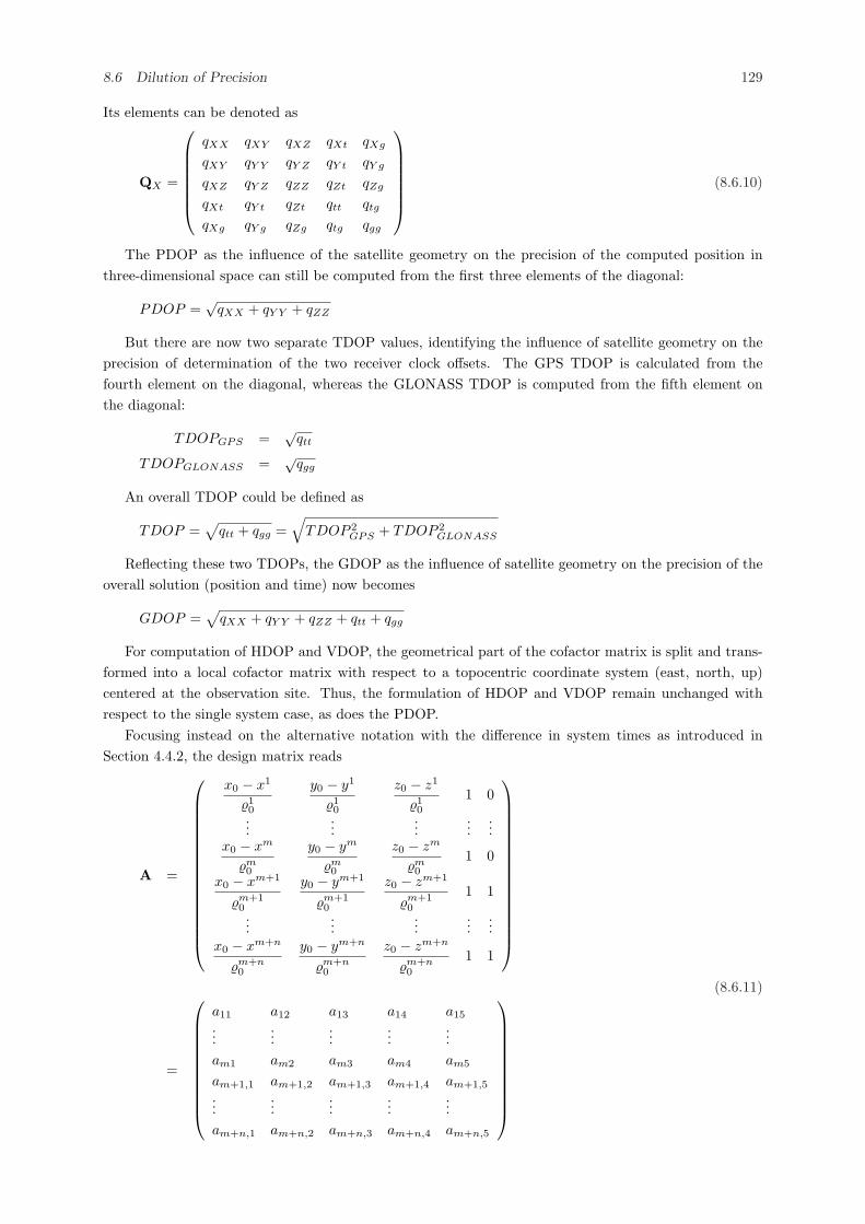
8.6 Dilution of Precision 129
Its elements can be denoted as
QX =
qXX qXY qXZ qXt qXg
qXY qY Y qY Z qY t qY g
qXZ qY Z qZZ qZt qZg
qXt qY t qZt qtt qtg
qXg qY g qZg qtg qgg
(8.6.10)
The PDOP as the influence of the satellite geometry on the precision of the computed position inthree-dimensional space can still be computed from the first three elements of the diagonal:
PDOP =√
qXX + qY Y + qZZ
But there are now two separate TDOP values, identifying the influence of satellite geometry on theprecision of determination of the two receiver clock offsets. The GPS TDOP is calculated from thefourth element on the diagonal, whereas the GLONASS TDOP is computed from the fifth element onthe diagonal:
TDOPGPS =√
qtt
TDOPGLONASS =√
qgg
An overall TDOP could be defined as
TDOP =√
qtt + qgg =√
TDOP 2GPS + TDOP 2
GLONASS
Reflecting these two TDOPs, the GDOP as the influence of satellite geometry on the precision of theoverall solution (position and time) now becomes
GDOP =√
qXX + qY Y + qZZ + qtt + qgg
For computation of HDOP and VDOP, the geometrical part of the cofactor matrix is split and trans-formed into a local cofactor matrix with respect to a topocentric coordinate system (east, north, up)centered at the observation site. Thus, the formulation of HDOP and VDOP remain unchanged withrespect to the single system case, as does the PDOP.
Focusing instead on the alternative notation with the difference in system times as introduced inSection 4.4.2, the design matrix reads
A =
x0 − x1
%10
y0 − y1
%10
z0 − z1
%10
1 0
......
......
...x0 − xm
%m0
y0 − ym
%m0
z0 − zm
%m0
1 0
x0 − xm+1
%m+10
y0 − ym+1
%m+10
z0 − zm+1
%m+10
1 1
......
......
...x0 − xm+n
%m+n0
y0 − ym+n
%m+n0
z0 − zm+n
%m+n0
1 1
(8.6.11)
=
a11 a12 a13 a14 a15
......
......
...am1 am2 am3 am4 am5
am+1,1 am+1,2 am+1,3 am+1,4 am+1,5
......
......
...am+n,1 am+n,2 am+n,3 am+n,4 am+n,5
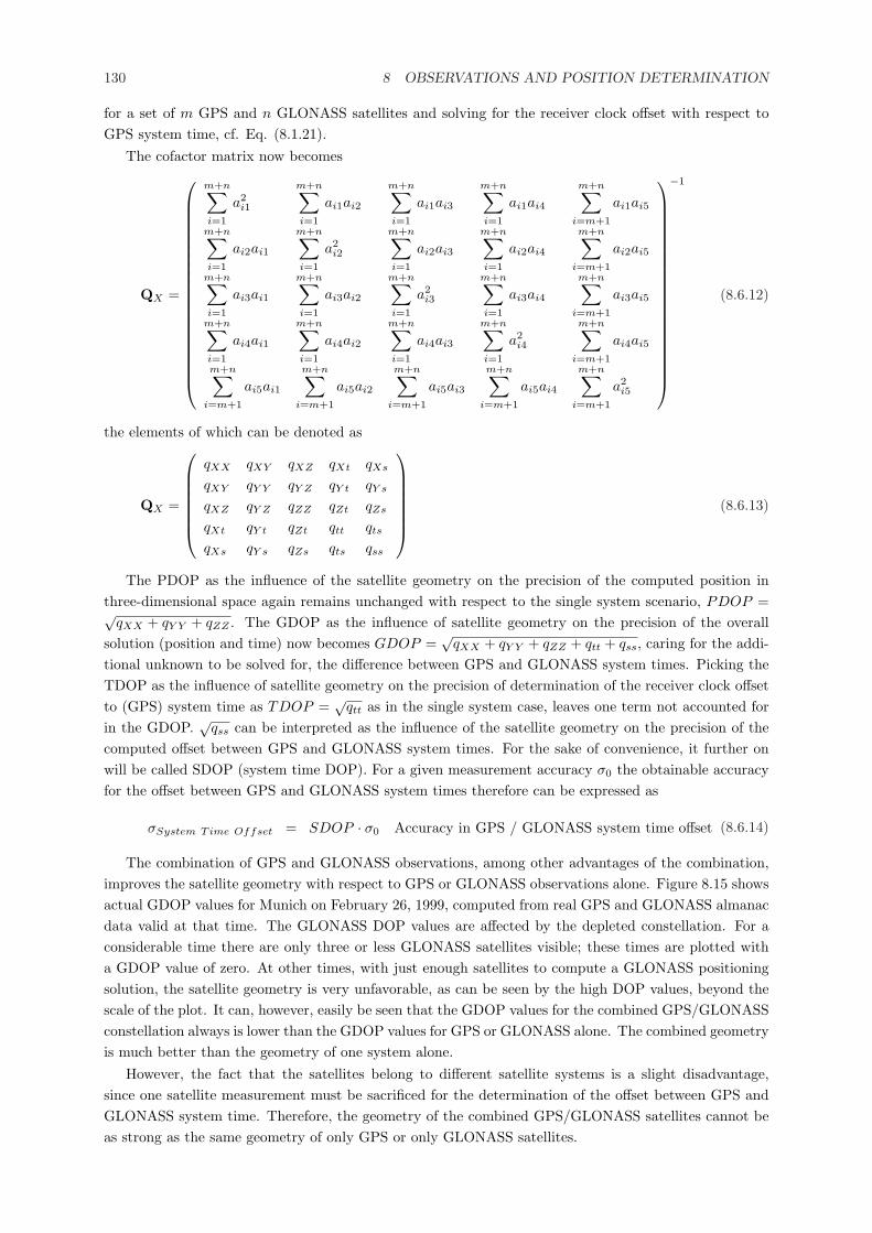
130 8 OBSERVATIONS AND POSITION DETERMINATION
for a set of m GPS and n GLONASS satellites and solving for the receiver clock offset with respect toGPS system time, cf. Eq. (8.1.21).
The cofactor matrix now becomes
QX =
m+n∑
i=1
a2i1
m+n∑
i=1
ai1ai2
m+n∑
i=1
ai1ai3
m+n∑
i=1
ai1ai4
m+n∑
i=m+1
ai1ai5
m+n∑
i=1
ai2ai1
m+n∑
i=1
a2i2
m+n∑
i=1
ai2ai3
m+n∑
i=1
ai2ai4
m+n∑
i=m+1
ai2ai5
m+n∑
i=1
ai3ai1
m+n∑
i=1
ai3ai2
m+n∑
i=1
a2i3
m+n∑
i=1
ai3ai4
m+n∑
i=m+1
ai3ai5
m+n∑
i=1
ai4ai1
m+n∑
i=1
ai4ai2
m+n∑
i=1
ai4ai3
m+n∑
i=1
a2i4
m+n∑
i=m+1
ai4ai5
m+n∑
i=m+1
ai5ai1
m+n∑
i=m+1
ai5ai2
m+n∑
i=m+1
ai5ai3
m+n∑
i=m+1
ai5ai4
m+n∑
i=m+1
a2i5
−1
(8.6.12)
the elements of which can be denoted as
QX =
qXX qXY qXZ qXt qXs
qXY qY Y qY Z qY t qY s
qXZ qY Z qZZ qZt qZs
qXt qY t qZt qtt qts
qXs qY s qZs qts qss
(8.6.13)
The PDOP as the influence of the satellite geometry on the precision of the computed position inthree-dimensional space again remains unchanged with respect to the single system scenario, PDOP =√
qXX + qY Y + qZZ . The GDOP as the influence of satellite geometry on the precision of the overallsolution (position and time) now becomes GDOP =
√qXX + qY Y + qZZ + qtt + qss, caring for the addi-
tional unknown to be solved for, the difference between GPS and GLONASS system times. Picking theTDOP as the influence of satellite geometry on the precision of determination of the receiver clock offsetto (GPS) system time as TDOP =
√qtt as in the single system case, leaves one term not accounted for
in the GDOP.√
qss can be interpreted as the influence of the satellite geometry on the precision of thecomputed offset between GPS and GLONASS system times. For the sake of convenience, it further onwill be called SDOP (system time DOP). For a given measurement accuracy σ0 the obtainable accuracyfor the offset between GPS and GLONASS system times therefore can be expressed as
σSystem Time Offset = SDOP · σ0 Accuracy in GPS / GLONASS system time offset (8.6.14)
The combination of GPS and GLONASS observations, among other advantages of the combination,improves the satellite geometry with respect to GPS or GLONASS observations alone. Figure 8.15 showsactual GDOP values for Munich on February 26, 1999, computed from real GPS and GLONASS almanacdata valid at that time. The GLONASS DOP values are affected by the depleted constellation. For aconsiderable time there are only three or less GLONASS satellites visible; these times are plotted witha GDOP value of zero. At other times, with just enough satellites to compute a GLONASS positioningsolution, the satellite geometry is very unfavorable, as can be seen by the high DOP values, beyond thescale of the plot. It can, however, easily be seen that the GDOP values for the combined GPS/GLONASSconstellation always is lower than the GDOP values for GPS or GLONASS alone. The combined geometryis much better than the geometry of one system alone.
However, the fact that the satellites belong to different satellite systems is a slight disadvantage,since one satellite measurement must be sacrificed for the determination of the offset between GPS andGLONASS system time. Therefore, the geometry of the combined GPS/GLONASS satellites cannot beas strong as the same geometry of only GPS or only GLONASS satellites.
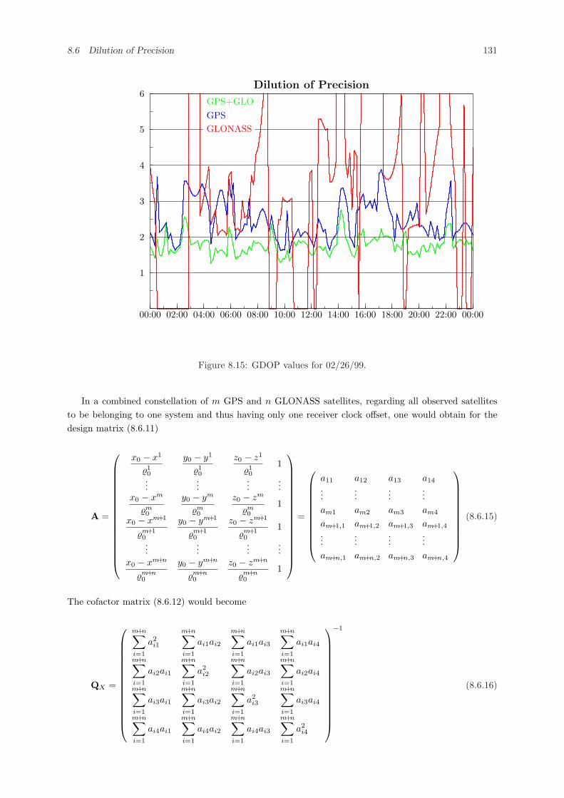
8.6 Dilution of Precision 131
00:00 02:00 04:00 06:00 08:00 10:00 12:00 14:00 16:00 18:00 20:00 22:00 00:00
1
2
3
4
5
6Dilution of Precision
GPS+GLOGPSGLONASS
Figure 8.15: GDOP values for 02/26/99.
In a combined constellation of m GPS and n GLONASS satellites, regarding all observed satellitesto be belonging to one system and thus having only one receiver clock offset, one would obtain for thedesign matrix (8.6.11)
A =
x0 − x1
%10
y0 − y1
%10
z0 − z1
%10
1
......
......
x0 − xm
%m0
y0 − ym
%m0
z0 − zm
%m0
1
x0 − xm+1
%m+10
y0 − ym+1
%m+10
z0 − zm+1
%m+10
1
......
......
x0 − xm+n
%m+n0
y0 − ym+n
%m+n0
z0 − zm+n
%m+n0
1
=
a11 a12 a13 a14
......
......
am1 am2 am3 am4
am+1,1 am+1,2 am+1,3 am+1,4
......
......
am+n,1 am+n,2 am+n,3 am+n,4
(8.6.15)
The cofactor matrix (8.6.12) would become
QX =
m+n∑
i=1
a2i1
m+n∑
i=1
ai1ai2
m+n∑
i=1
ai1ai3
m+n∑
i=1
ai1ai4
m+n∑
i=1
ai2ai1
m+n∑
i=1
a2i2
m+n∑
i=1
ai2ai3
m+n∑
i=1
ai2ai4
m+n∑
i=1
ai3ai1
m+n∑
i=1
ai3ai2
m+n∑
i=1
a2i3
m+n∑
i=1
ai3ai4
m+n∑
i=1
ai4ai1
m+n∑
i=1
ai4ai2
m+n∑
i=1
ai4ai3
m+n∑
i=1
a2i4
−1
(8.6.16)
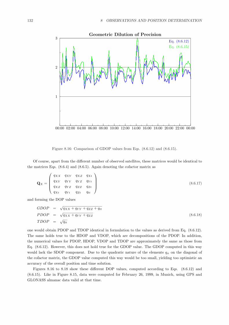
132 8 OBSERVATIONS AND POSITION DETERMINATION
00:00 02:00 04:00 06:00 08:00 10:00 12:00 14:00 16:00 18:00 20:00 22:00 00:00
1
2
3Geometric Dilution of Precision
Eq. (8.6.12)Eq. (8.6.15)
Figure 8.16: Comparison of GDOP values from Eqs. (8.6.12) and (8.6.15).
Of course, apart from the different number of observed satellites, these matrices would be identical tothe matrices Eqs. (8.6.4) and (8.6.5). Again denoting the cofactor matrix as
QX =
qXX qXY qXZ qXt
qXY qY Y qY Z qY t
qXZ qY Z qZZ qZt
qXt qY t qZt qtt
(8.6.17)
and forming the DOP values
GDOP =√
qXX + qY Y + qZZ + qtt
PDOP =√
qXX + qY Y + qZZ (8.6.18)
TDOP =√
qtt
one would obtain PDOP and TDOP identical in formulation to the values as derived from Eq. (8.6.12).The same holds true to the HDOP and VDOP, which are decompositions of the PDOP. In addition,the numerical values for PDOP, HDOP, VDOP and TDOP are approximately the same as those fromEq. (8.6.12). However, this does not hold true for the GDOP value. The GDOP computed in this waywould lack the SDOP component. Due to the quadratic nature of the elements qii on the diagonal ofthe cofactor matrix, the GDOP value computed this way would be too small, yielding too optimistic anaccuracy of the overall position and time solution.
Figures 8.16 to 8.18 show these different DOP values, computed according to Eqs. (8.6.12) and(8.6.15). Like in Figure 8.15, data were computed for February 26, 1999, in Munich, using GPS andGLONASS almanac data valid at that time.
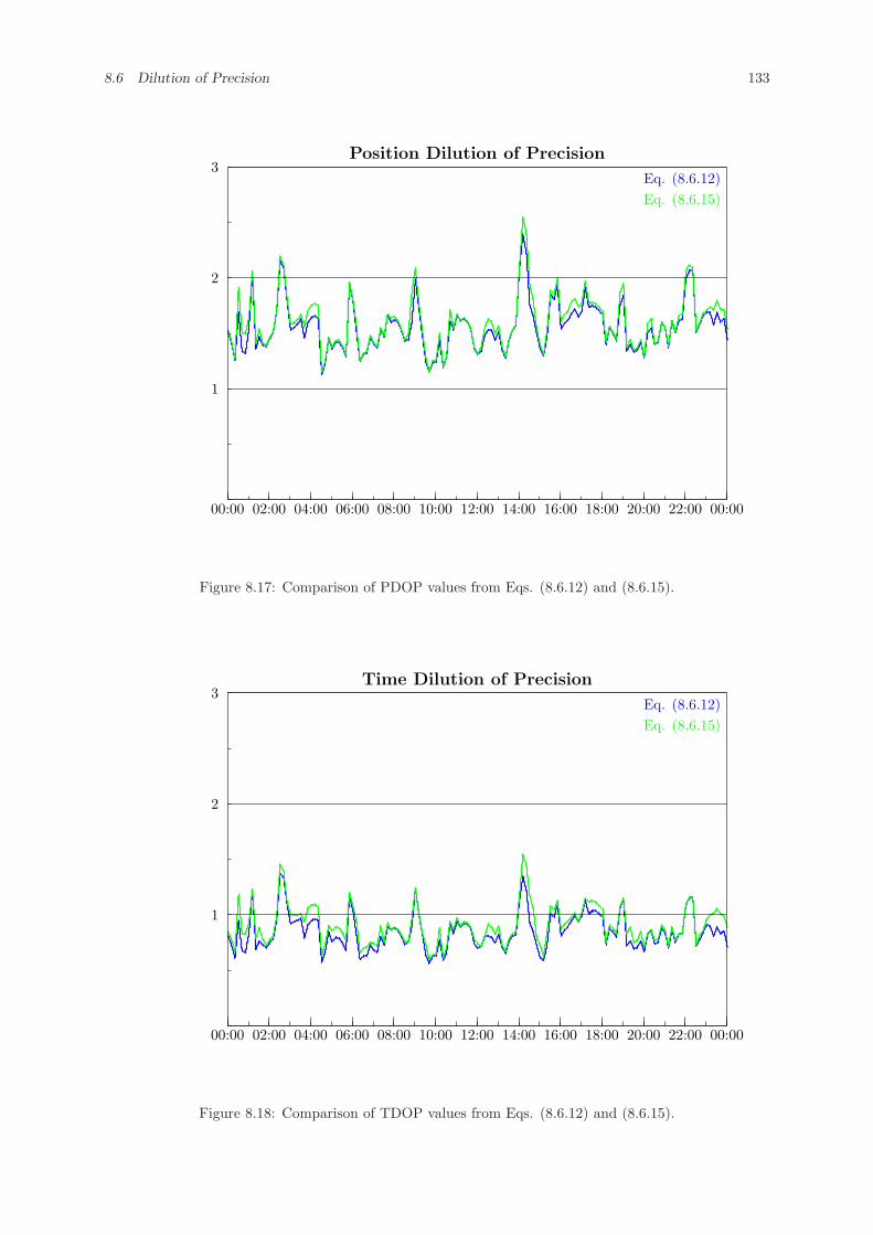
8.6 Dilution of Precision 133
00:00 02:00 04:00 06:00 08:00 10:00 12:00 14:00 16:00 18:00 20:00 22:00 00:00
1
2
3Position Dilution of Precision
Eq. (8.6.12)Eq. (8.6.15)
Figure 8.17: Comparison of PDOP values from Eqs. (8.6.12) and (8.6.15).
00:00 02:00 04:00 06:00 08:00 10:00 12:00 14:00 16:00 18:00 20:00 22:00 00:00
1
2
3Time Dilution of Precision
Eq. (8.6.12)Eq. (8.6.15)
Figure 8.18: Comparison of TDOP values from Eqs. (8.6.12) and (8.6.15).

134 8 OBSERVATIONS AND POSITION DETERMINATION
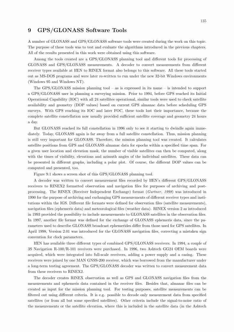
135
9 GPS/GLONASS Software Tools
A number of GLONASS and GPS/GLONASS software tools were created during the work on this topic.The purpose of these tools was to test and evaluate the algorithms introduced in the previous chapters.All of the results presented in this work were obtained using this software.
Among the tools created are a GPS/GLONASS planning tool and different tools for processing ofGLONASS and GPS/GLONASS measurements. A decoder to convert measurements from differentreceiver types available at IfEN to RINEX format also belongs to this software. All these tools startedout as MS-DOS programs and were later re-written to run under the new 32-bit Windows environments(Windows 95 and Windows NT).
The GPS/GLONASS mission planning tool – as is expressed in its name – is intended to supporta GPS/GLONASS user in planning a surveying mission. Prior to 1994, before GPS reached its InitialOperational Capability (IOC) with all 24 satellites operational, similar tools were used to check satelliteavailability and geometry (DOP values) based on current GPS almanac data before scheduling GPSsurveys. With GPS reaching its IOC and later FOC, these tools lost their importance, because thecomplete satellite constellation now usually provided sufficient satellite coverage and geometry 24 hoursa day.
But GLONASS reached its full constellation in 1996 only to see it starting to dwindle again imme-diately. Today, GLONASS again is far away from a full satellite constellation. Thus, mission planningis still very important for GLONASS. Therefore, the mission planning tool was created. It calculatessatellite positions from GPS and GLONASS almanac data for epochs within a specified time span. Fora given user location and elevation mask, the number of visible satellites can then be computed, alongwith the times of visibility, elevations and azimuth angles of the individual satellites. These data canbe presented in different graphs, including a polar plot. Of course, the different DOP values can becomputed and presented, too.
Figure 9.1 shows a screen shot of this GPS/GLONASS planning tool.
A decoder was written to convert measurement files recorded by IfEN’s different GPS/GLONASSreceivers to RINEX2 formatted observation and navigation files for purposes of archiving and post-processing. The RINEX (Receiver Independent Exchange) format (Gurtner, 1998) was introduced in1990 for the purpose of archiving and exchanging GPS measurements of different receiver types and insti-tutions within the IGS. Different file formats were defined for observation files (satellite measurements),navigation files (ephemeris data) and meteorological files (weather data). RINEX version 2 as introducedin 1993 provided the possibility to include measurements to GLONASS satellites in the observation files.In 1997, another file format was defined for the exchange of GLONASS ephemeris data, since the pa-rameters used to describe GLONASS broadcast ephemerides differ from those used for GPS satellites. InApril 1998, Version 2.01 was introduced for the GLONASS navigation files, correcting a mistaken signconvention for clock parameters.
IfEN has available three different types of combined GPS/GLONASS receivers. In 1994, a couple of3S Navigation R-100/R-101 receivers were purchased. In 1996, two Ashtech GG24 OEM boards wereacquired, which were integrated into full-scale receivers, adding a power supply and a casing. Thesereceivers were joined by one MAN GNSS-200 receiver, which was borrowed from the manufacturer undera long-term testing agreement. The GPS/GLONASS decoder was written to convert measurement datafrom these receivers to RINEX2.
The decoder creates RINEX observation as well as GPS and GLONASS navigation files from themeasurements and ephemeris data contained in the receiver files. Besides that, almanac files can becreated as input for the mission planning tool. For testing purposes, satellite measurements can befiltered out using different criteria. It is e.g. possible to decode only measurement data from specifiedsatellites (or from all but some specified satellites). Other criteria include the signal-to-noise ratio ofthe measurements or the satellite elevation, where this is included in the satellite data (in the Ashtech
136 9 GPS/GLONASS SOFTWARE TOOLS
GG24). Measurement data can also be filtered by frequency band and/or code. This way, e.g. onlyP-code measurements can be decoded, or only L1 C/A-code measurements, or only L2, or . . .
During a decoding run, the assignment of satellites to the different receiver hardware channels can bedisplayed, together with the number of decoded measurements.
Figure 9.2 shows a screen shot of the GPS/GLONASS decoder.A real-time version of the decoder reads data online from a receiver connected to a serial port and
creates RINEX files in specified intervals.The GPS/GLONASS processing tools were created to compute user positions from GPS and GLO-
NASS satellite observations, using different algorithms. The single point positioning tool computes po-sitions from observation data recorded at one site, whereas the differential positioning tool employsobservations recorded simultaneously at two sites to calculate the position of one receiver, while theother (reference) site is held fixed.
Similar to the RINEX decoder, satellites and measurements to participate in the positioning solutioncan be selected using a number of criteria, such as satellite number, SNR, elevation mask or frequencyband and code. In addition, a DOP threshold can be specified for minimum requirements on the satellitegeometry. For evaluating the influence of the coordinate transformation from PZ-90 to WGS84, differentcoordinate transformations can be applied to GLONASS satellite positions prior to computing the userposition.
Either raw pseudoranges, carrier-smoothed pseudoranges or carrier phase ranges (in the differentialtool) can be used to compute the receiver position. Computed positions are output epoch-wise in tabularform and in different graphs, e.g. as scatter plots, depicting the distribution of the positioning solutionsin the horizontal plane.
For testing different processing algorithms or formulations of the observation equations (e.g. singleor double difference processing), these algorithms can easily be implemented in this test software bymodifying the source code and re-compiling the software.
Figure 9.3 shows a screen shot of the GPS/GLONASS absolute positioning tool.
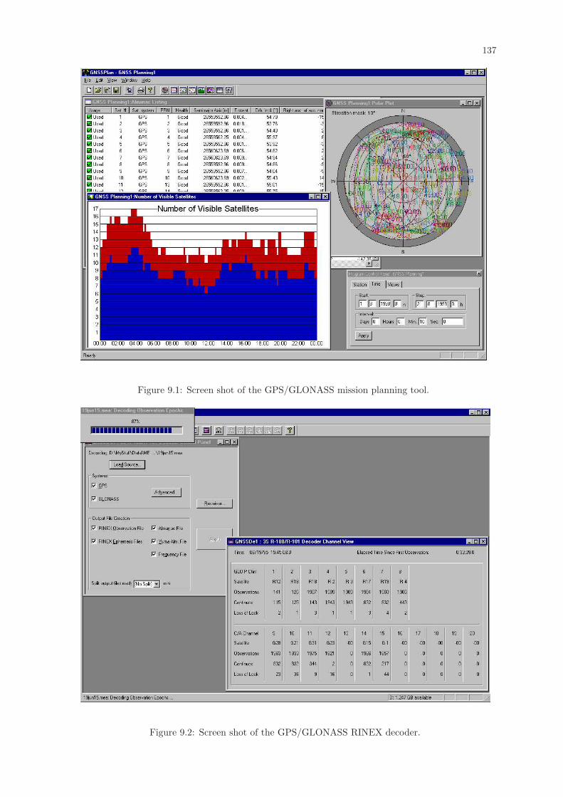
137
Figure 9.1: Screen shot of the GPS/GLONASS mission planning tool.
Figure 9.2: Screen shot of the GPS/GLONASS RINEX decoder.
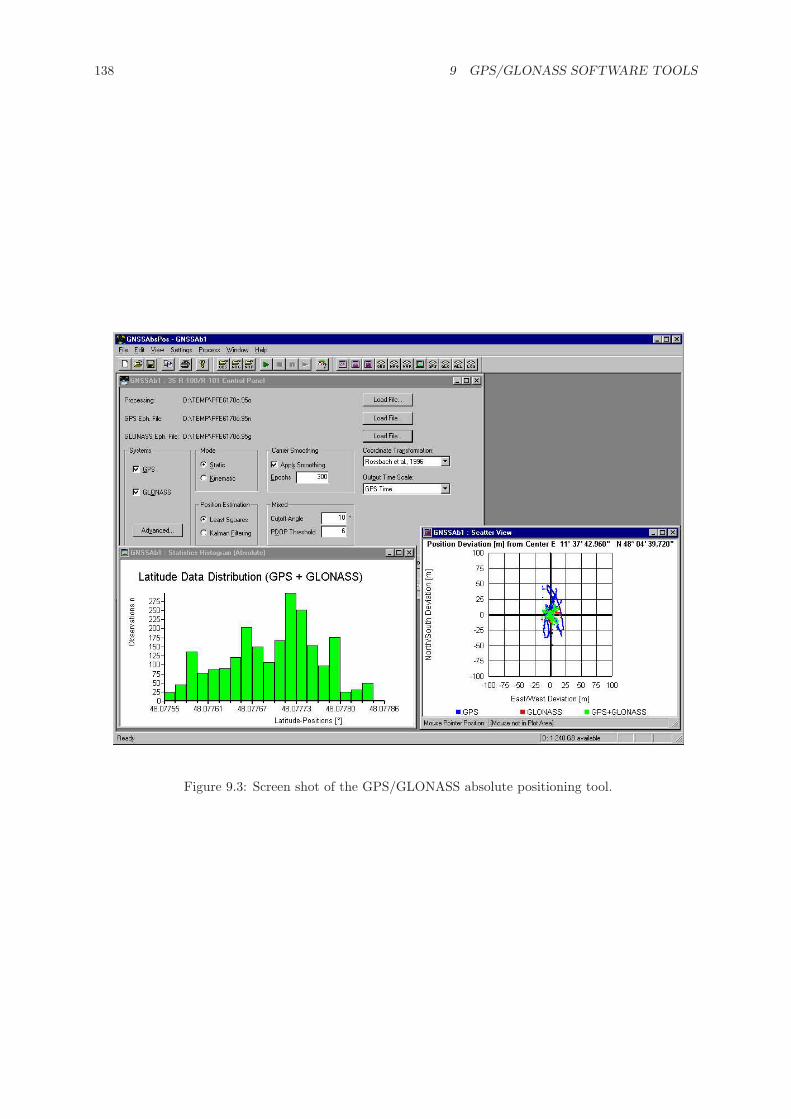
138 9 GPS/GLONASS SOFTWARE TOOLS
Figure 9.3: Screen shot of the GPS/GLONASS absolute positioning tool.
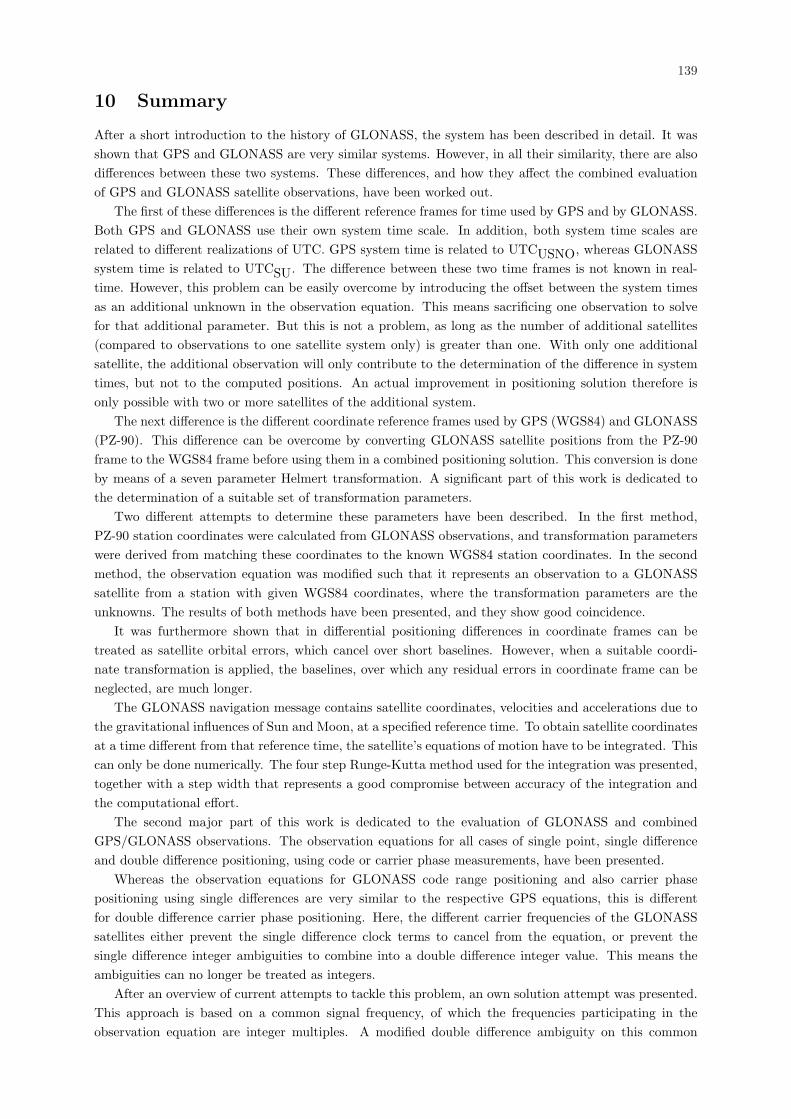
139
10 Summary
After a short introduction to the history of GLONASS, the system has been described in detail. It wasshown that GPS and GLONASS are very similar systems. However, in all their similarity, there are alsodifferences between these two systems. These differences, and how they affect the combined evaluationof GPS and GLONASS satellite observations, have been worked out.
The first of these differences is the different reference frames for time used by GPS and by GLONASS.Both GPS and GLONASS use their own system time scale. In addition, both system time scales arerelated to different realizations of UTC. GPS system time is related to UTCUSNO, whereas GLONASSsystem time is related to UTCSU. The difference between these two time frames is not known in real-time. However, this problem can be easily overcome by introducing the offset between the system timesas an additional unknown in the observation equation. This means sacrificing one observation to solvefor that additional parameter. But this is not a problem, as long as the number of additional satellites(compared to observations to one satellite system only) is greater than one. With only one additionalsatellite, the additional observation will only contribute to the determination of the difference in systemtimes, but not to the computed positions. An actual improvement in positioning solution therefore isonly possible with two or more satellites of the additional system.
The next difference is the different coordinate reference frames used by GPS (WGS84) and GLONASS(PZ-90). This difference can be overcome by converting GLONASS satellite positions from the PZ-90frame to the WGS84 frame before using them in a combined positioning solution. This conversion is doneby means of a seven parameter Helmert transformation. A significant part of this work is dedicated tothe determination of a suitable set of transformation parameters.
Two different attempts to determine these parameters have been described. In the first method,PZ-90 station coordinates were calculated from GLONASS observations, and transformation parameterswere derived from matching these coordinates to the known WGS84 station coordinates. In the secondmethod, the observation equation was modified such that it represents an observation to a GLONASSsatellite from a station with given WGS84 coordinates, where the transformation parameters are theunknowns. The results of both methods have been presented, and they show good coincidence.
It was furthermore shown that in differential positioning differences in coordinate frames can betreated as satellite orbital errors, which cancel over short baselines. However, when a suitable coordi-nate transformation is applied, the baselines, over which any residual errors in coordinate frame can beneglected, are much longer.
The GLONASS navigation message contains satellite coordinates, velocities and accelerations due tothe gravitational influences of Sun and Moon, at a specified reference time. To obtain satellite coordinatesat a time different from that reference time, the satellite’s equations of motion have to be integrated. Thiscan only be done numerically. The four step Runge-Kutta method used for the integration was presented,together with a step width that represents a good compromise between accuracy of the integration andthe computational effort.
The second major part of this work is dedicated to the evaluation of GLONASS and combinedGPS/GLONASS observations. The observation equations for all cases of single point, single differenceand double difference positioning, using code or carrier phase measurements, have been presented.
Whereas the observation equations for GLONASS code range positioning and also carrier phasepositioning using single differences are very similar to the respective GPS equations, this is differentfor double difference carrier phase positioning. Here, the different carrier frequencies of the GLONASSsatellites either prevent the single difference clock terms to cancel from the equation, or prevent thesingle difference integer ambiguities to combine into a double difference integer value. This means theambiguities can no longer be treated as integers.
After an overview of current attempts to tackle this problem, an own solution attempt was presented.This approach is based on a common signal frequency, of which the frequencies participating in theobservation equation are integer multiples. A modified double difference ambiguity on this common
140 10 SUMMARY
frequency can then be formed. This double difference is still an integer value. However, the draw-back ofthis solution is the small wavelength of this common frequency, resulting in large ambiguity values thatare difficult to fix. But on the other hand, due to that small wavelength it is not required to really fixthe ambiguities to integers. A fixing to thousands of integers may be sufficient.
The peculiarities of ionospheric correction and DOP computation for GLONASS and GPS/GLONASScombination are pointed out. The presence of two system time scales in combined GPS/GLONASS posi-tioning brings up an additional DOP value. Depending on the formulation of the observation equations,this can either be interpreted as an additional TDOP value, or as a DOP value associated with thedifference in system time scales.
Finally, a bundle of GPS/GLONASS software tools has been described that was designed within thescope of this work. These tools have been used to obtain the results presented herein.
141
Appendix
A Bibliography
3S Navigation (1994). R-100 Series GPS/GLONASS Receiver User’s Manual. 3S Navigation, LagunaHills, CA.
3S Navigation (1996a). GNSS-200 GPS/GLONASS Receiver User’s Manual. 3S Navigation / MANTechnologie AG, Laguna Hills, CA.
3S Navigation (1996b). GNSS-300 GPS/GLONASS Receiver User’s Manual. 3S Navigation / MANTechnologie AG, Laguna Hills, CA.
Abusali, P. A. M., Schutz, B. E., Tapley, B. D., and Bevis, M. (1995). Transformation between SLR/VLBIand WGS-84 Reference Frames. Bulletin Geodesique, 69:61–72.
Anodina, T. G. (1988). GLONASS System Technical Characteristics and Performance. Working PapersWP/70 and WP/75, Special Committee on Future Air Navigation Systems (FANS/4), InternationalCivil Aviation Organization (ICAO), Montreal.
Ashtech (1996). GG24 GPS+GLONASS Receiver Reference Manual. Ashtech Inc., Sunnyvale, CA.
Ashtech (1998a). WWW Home Page. Ashtech Inc., Sunnyvale, CA. http://www.ashtech.com.
Ashtech (1998b). Z-18 GPS+GLONASS Receiver Data Sheet. Ashtech Inc., Sunnyvale, CA.
Balendra, A., Kim, S., and Beser, J. (1994). Fully Integrated GLONASS Dual Frequency P Code andGPS/GLONASS Single Frequency C/A Code Receiver. In Proceedings of ION Satellite DivisionGPS-94 International Technical Meeting, pages 461–470, Salt Lake City, Utah.
Bartenev, V. A. et al. (1994). The GLONASS Global Positioning System.
Bazlov, Y. A., Galazin, V. F., Kaplan, B. L., Maksimov, V. G., and Rogozin, V. P. (1999). GLONASSto GPS: A New Coordinate Transformation. GPS World Magazine, 10(1):54–58.
Beser, J. and Danaher, J. (1993). The 3S Navigation R-100 Family of Integrated GPS/GLONASSReceivers: Description and Performance Results. In Proceedings of ION Satellite Division NationalTechnical Meeting, San Francisco, California.
Beutler, G., Bauersima, I., Gurtner, W., Rothacher, M., and Schildknecht, T. (1987). AtmosphericRefraction and Other Important Biases in GPS Carrier Phase Observations. Internal Report 22,”Satellitenbeobachtungsstation Zimmerwald”, Bern, Switzerland.
BIPM (1995). Annual Report of the BIPM Time Section, Volume 8. Technical report, BIPM, Pavillonde Breteuil.
Boykov, V. V. et al. (1993). Experimental Compiling the Geocentric System of Coordinates PZ-90 (inRussian Language). Geodezia i Kartografia, 11:17 – 21.Bo$ikov, V. V. i dr.: Opyt sozdani� geocentriqesko$i sistemy koordinat PZ-90, v ”Geode-si� i kartografia”, N 11, no�br~ 1993, str. 17 - 21.
CCDS (1996). Recommendation S4 (1996) ”Coordination of Satellite Systems Providing Timing”. Reportof the 13th Meeting of the CCDS, Comite Consultatif pour la Definition de la Seconde, BIPM.
CDISS (1998). WWW Home Page. Centre for Defence & International Security Studies, LancasterUniversity, Lancaster, UK. http://www.cdiss.org/mos as3.htm.
142 A BIBLIOGRAPHY
Cook, A. H. (1977). Celestial Masers. Cambridge University Press, Cambridge.
Cook, G. L. (1997). Critical GPS-GLONASS Interoperability Issues. In Proceedings of ION SatelliteDivision National Technical Meeting, pages 183–193, Santa Monica, California.
CSIC (1994). GLONASS Info, Bulletin 1/94 (1). Coordinational Scientific Information Center RussianSpace Forces, Moscow. English Translation of Russian Document.
CSIC (1997). Notice Advisory to GLONASS Users, No. 052-970619. Coordinational Scientific InformationCenter Russian Space Forces.
CSIC (1998). GLONASS WWW Home Page. Coordinational Scientific Information Center Russian SpaceForces, Moscow. http://mx.iki.rssi.ru/SFCSIC/english.html.
Dale, S. A., Daly, P., and Kitching, I. D. (1989). Understanding Signals From GLONASS NavigationSatellites. International Journal of Satellite Communications, 7:11–22.
Dale, S. A., Kitching, I. D., and Daly, P. (1988). Position-Fixing Using the USSR’s GLONASS C/ACode. In Proceedings of IEEE Position Location & Navigation Symposium, PLANS’88, pages 13–20.
DASA (1996). ASN-22 GPS/GLONASS Receiver Data Sheet. DASA–NFS.
Eastwood, R. A. (1990). An Integrated GPS/GLONASS Receiver. Navigation: Journal of The Instituteof Navigation, 37(2):141–151.
Felhauer, T., Tews, T., Botchkovski, A., Golubev, M., and Vasilyev, M. (1997). ASN-22 CombinedGPS/GLONASS Receiver Module – Architecture, Technical Characteristics and Performance Anal-ysis. In Proceedings of ION Satellite Division GPS-97 International Technical Meeting, pages 81–87,Kansas City, Missouri.
Ganin, A. (1995). Differential GLONASS in Russia: The Ways of Development. In Proceedings ofION Satellite Division GPS-95 International Technical Meeting, pages 1049–1052, Palm Springs,California.
Gourevitch, S. A., Sila-Novitsky, S., and Diggelen, F. v. (1996). The GG24 Combined GPS+GLONASSReceiver. In Proceedings of ION Satellite Division GPS-96 International Technical Meeting, pages141–145, Kansas City, Missouri.
Gouzhva, Y. G., Gevorkyan, A. G., Bogdanov, P. P., Ovchinnikov, V. V., and Pushkina, I. G. (1995).Getting in Sync: GLONASS Clock Synchronization. GPS World Magazine, 6(4):48–56.
Government (1995). On executing works in use of the GLONASS global navigation satellite system forthe sake of civil users. The Government of the Russian Federation, Decree No. 237.
Government (1997). On Federal aim program of using GLONASS global navigation satellite system forthe benefits of civil users. The Government of the Russian Federation, Decree No. 1435.
GPNN (1994). Global Positioning & Navigation News, Vol. 4, No. 16, Phillips Business Information,Washington, D. C.
Graas, Frank, v. and Braasch, M. S. (1996). Selective Availability. In Parkinson, B. W. and Spilker,jr., J. J., editors, Global Positioning System: Theory and Applications I, volume 163 of Progress inAstronautics and Aeronautics, pages 601–622. American Institute of Aeronautics and Astronautics,Washington, D. C., USA.
Gurtner, W. (1998). RINEX: The Receiver Independent Exchange Format Version 2. Format definition,Astronomical Institute, University of Berne, Berne. Definition file available on IGS WWW Siteftp://igscb.jpl.nasa.gov/igscb/data/format/rinex2.txt.
143
Habrich, H. (1999). Geodetic Applications of the Global Navigation Satellite System (GLONASS) and ofGLONASS/GPS Combinations. PhD thesis, University of Berne, Department for Philosophy andNatural Sciences, Berne, Switzerland.
Habrich, H., Beutler, G., Gurtner, W., and Rothacher, M. (1999). Double Difference Ambiguity Resolu-tion for GLONASS/GPS Carrier Phase. In Proceedings of ION Satellite Division GPS-99 Interna-tional Technical Meeting, pages 1609–1618, Nashville, Tennessee.
Hartmann, R. (1992). Joint US/USSR Satellite Navigation Studies. GPS World Magazine, 3(2):26–36.
Hein, G. W., Pielmeier, J., Zink, T., Eißfeller, B., Perry, M., and Rawlings, R. (1997). GPS andGLONASS RAIM Availability Analysis Over Europe. In Proceedings of ION Satellite Division GPS-97 International Technical Meeting, pages 465–475, Kansas City, Missouri.
Heinrichs, G. and Gotz, S. (1996). The GNSS-200: Features and Performance of the Fully IntegratedSingle Frequency, 12 Channel, C/A Code GPS/GLONASS Receiver. In Proceedings of ION SatelliteDivision GPS-96 International Technical Meeting, pages 125–130, Kansas City, Missouri.
Heinrichs, G., Gotz, S., and Windl, J. (1997). The NR - Navigation System Family: Features and Perfor-mance of the Fully Integrated Single Frequency, 24 Channel, C/A Code GPS/GLONASS NavigationSystems. In Proceedings of ION Satellite Division GPS-97 International Technical Meeting, pages61–67, Kansas City, Missouri.
Heiskanen, W. and Moritz, H. (1967). Physical Geodesy. W H Freeman, San Francisco.
Hofmann-Wellenhof, B., Lichtenegger, H., and Collins, J. (1993). Global Positioning System – Theoryand Practice. Springer Verlag, Wien, New York, 2nd edition.
ICAO (1996). Letter from the President of the ICAO Council to the Russian Minister of Transport,Montreal, July 29.
ICD-GLONASS (1995). GLONASS Interface Control Document (Rev. 1995). Coordinational ScientificInformation Center Russian Space Forces, Moscow. English Translation of Russian Document.
ICD-GLONASS (1998). GLONASS Interface Control Document (Version 4.0). Coordinational ScientificInformation Center Russian Space Forces, Moscow. English Translation of Russian Document.
ICD-GPS (1991). GPS Interface Control Document (ICD-GPS-200). ARINC Research Corporation.
IGN (1998). IGEX-98 WWW Home Page. Institut Geographique Nationale, Paris, France. http://
lareg.ensg.ign.fr/IGEX/.
ISDE (1991a). ”Gnom” GLONASS Receiver Data Sheet. Institute of Space Device Engineering, Moscow.
ISDE (1991b). ”Reper” GPS/GLONASS Receiver Data Sheet. Institute of Space Device Engineering,Moscow.
Ivanov, N. E., Salischev, V., and Vinogradov, A. (1995). Ways of GLONASS System Advancing. InProceedings of ION Satellite Division GPS-95 International Technical Meeting, pages 991–1011,Palm Springs, California.
Jansche, A. M. (1993). GLONASS – A Summary. Technical report, Kayser-Threde GmbH, Munich.
Javad (1998). WWW Home Page. Javad Positioning Systems, San Jose, CA, USA. http://www.
javad.com.
Jeltsch, R. (1987). Numerische Mathematik I fur Ingenieure. Rheinisch-Westfalische TechnischeHochschule Aachen, Aachen. Lecture notes.
144 A BIBLIOGRAPHY
Johnson, N. L. (1994). GLONASS Spacecraft. GPS World Magazine, 5(11):51–58.
Kayser-Threde (1991a). ASN-16 GLONASS Receiver Data Sheet. Kayser-Threde GmbH, Munich.
Kayser-Threde (1991b). ”Skipper” GLONASS Receiver Data Sheet. Kayser-Threde GmbH, Munich.
Kazantsev, V. (1995). The GLONASS and GLONASS-M Programs. In Proceedings of ION SatelliteDivision GPS-95 International Technical Meeting, pages 985–990, Palm Springs, California.
Kowalski, G. (1995). Plessezk macht zivile Karriere. Flug Revue 3/95, page 42.
Kozlov, D. and Tkachenko, M. (1998). Centimeter-Level, Real-Time Kinematic Positioning with GPS +GLONASS C/A Receivers. Navigation: Journal of The Institute of Navigation, 45(2):137–147.
Landau, H. and Vollath, U. (1996). Carrier Phase Ambiguity Resolution using GPS and GLONASSSignals. In Proceedings of ION Satellite Division GPS-96 International Technical Meeting, pages917–923, Kansas City, Missouri.
Langley, R. B. (1997). GLONASS Review and Update. GPS World Magazine, 8(7):46–51.
Leick, A., Li, J., Beser, J., and Mader, G. (1995). Processing GLONASS Carrier Phase Observations– Theory and First Experience. In Proceedings of ION Satellite Division GPS-95 InternationalTechnical Meeting, pages 1041–1047, Palm Springs, California.
Leisten, O., Ffoulkes-Jones, G., Whitworth, G., and Belton, D. (1995). Tracking Measurements Froma Miniature GLONASS Receiver. In Proceedings of ION Satellite Division GPS-95 InternationalTechnical Meeting, pages 853–859, Palm Springs, California.
Lennen, G. R. (1989). The USSR’s Glonass P-Code – Determination and Initial Results. In Proceedingsof ION Satellite Division GPS-89 International Technical Meeting, pages 77–83, Colorado Springs,Colorado.
Lewandowski, W. and Azoubib, J. (1998). GPS+GLONASS: Toward Subnanosecond Time Transfer.GPS World Magazine, 9(11):30–39.
Lewandowski, W., Azoubib, J., Jong, G. d., Nawrocki, J., and Danaher, J. (1997). A New Approachto International Satellite Time and Frequency Comparisons: ’All-in-View’ Multichannel GPS +GLONASS Observations. In Proceedings of ION Satellite Division GPS-97 International TechnicalMeeting, pages 1085–1091, Kansas City, Missouri.
Lewandowski, W., Danaher, J., and Klepczynski, W. J. (1996). Experiment Using GPS/GLONASSCommon View Time Transfer Between Europe and North America. In Proceedings of ION SatelliteDivision GPS-96 International Technical Meeting, pages 271–277, Kansas City, Missouri. Instituteof Navigation.
Litvak, M. M. (1969). Infra-red pumping of interstellar OH. Astrophysical Journal, 156:471–492.
Milliken, R. J. and Zoller, C. J. (1996). Principle of operation of NAVSTAR and system characteristics.In Global Positioning System, volume 1, pages 3–14. The Institute of Navigation.
Misra, P. N. and Abbot, R. I. (1994). SGS-85 – WGS84 Transformation. manuscripta geodaetica, 19:300–308.
Misra, P. N., Abbot, R. I., and Gaposchkin, E. M. (1996a). Integrated Use of GPS and GLONASS: PZ-90– WGS84 Transformation. In Proceedings of ION Satellite Division GPS-96 International TechnicalMeeting, pages 307–314, Kansas City, Missouri.
145
Misra, P. N., Bayliss, E. T., LaFrey, R. R., Pratt, M. M., and Hogaboom, R. A. (1992). GLONASS DataAnalysis: Interim Results. Navigation: Journal of The Institute of Navigation, 39(1):93–109.
Misra, P. N., Bayliss, E. T., LaFrey, R. R., Pratt, M. M., Hogaboom, R. A., and Muchnik, R. (1993).GLONASS Performance in 1992: A Review. GPS World Magazine, 4(5):28–38.
Misra, P. N., Pratt, M. M., Muchnik, R., Burke, B., and Hall, T. (1996b). GLONASS Performance:Measurement Data Quality and System Upkeep. In Proceedings of ION Satellite Division GPS-96International Technical Meeting, pages 261–270, Kansas City, Missouri.
Mitrikas, V. V., Revnivykh, S. G., and Bykhanov, E. V. (1998). WGS84/PZ-90 Transformation Parame-ters Determination Based on Laser and Ephemeris Long-Term GLONASS Orbital Data Processing.In Proceedings of ION Satellite Division GPS-98 International Technical Meeting, pages 1625–1635,Nashville, Tennessee.
MMC (1996). Press Release, Main Metrological Center of the National Time and Frequency Service ofthe Russian Federation.
NASA (1998). WWW Home Page on Russian Space Agency launch facilities. National Aeronautics andSpace Administration. http://liftoff.msfc.nasa.gov/rsa/pads.html.
NIMA (1997). Department of Defense World Geodetic System 1984, Its Definition and Relationships withLocal Geodetic Systems. National Imagery and Mapping Agency, Bethesda, Maryland, 3rd edition.Report No. 8350.2.
N.N. (1990a). DoD Turns On Selective Availability. GPS World Magazine, 1(3):12 (Global View).
N.N. (1990b). GPS/GLONASS Activity Gains Momentum. GPS World Magazine, 1(5):12 (Global View).
N.N. (1990c). GPS/GLONASS Cooperative Effort Moves Forward. GPS World Magazine, 1(1):18 (GlobalView).
N.N. (1990d). Northwest/Honeywell Sign Memorandum with Soviets on GPS/GLONASS. GPS WorldMagazine, 1(4):13 (Global View).
N.N. (1992). WARC Okays ’Shared Use’ of GLONASS Frequencies. GPS World Magazine, 3(4):22(Global View).
N.N. (1993a). European Initiatives Press for Civil System. GPS World Magazine, 4(3):24 (Global View).
N.N. (1993b). Visit to GLONASS Center is First for Outsiders. GPS World Magazine, 4(9):16 (GlobalView).
NovAtel (1998a). MiLLenium–GLONASS GPS+GLONASS Receiver Data Sheet. NovAtel Inc., Calgary,Alberta, Canada.
NovAtel (1998b). WWW Home Page. NovAtel Inc., Calgary, Alberta, Canada. http://www.
novatel.com.
Raby, P. and Daly, P. (1993). Using the GLONASS System for Geodetic Survey. In Proceedings of IONSatellite Division GPS-93 International Technical Meeting, pages 1129–1138, Salt Lake City, Utah.
RAG (1998). WWW Home Page. Russian Aerospace Guide, Roselle, IL. http://www.mcs.net/
~rusaerog/.
Revnivykh, S. G. and Mitrikas, V. V. (1998). GLONASS S/C mass and dimension. E-Mail throughIGEXMail service.
146 A BIBLIOGRAPHY
Riley, S. (1992). An Integrated Multichannel GPS/GLONASS Receiver. In Proceedings of ION SatelliteDivision GPS-92 International Technical Meeting, Albuquerque, New Mexico.
Riley, S. and Daly, P. (1994). Performance of the GLONASS P-code at L1 and L2 Frequencies. Interna-tional Journal of Satellite Communication, 12:453–462.
Riley, S. and Daly, P. (1995). Architecture and Results from the Leeds University 20 Channel GNSSReceiver. In Proceedings of ION Satellite Division National Technical Meeting, pages 421–430,Anaheim, California.
Riley, S., Howard, N., Aardom, E., Daly, P., and Silvestrin, P. (1995). A Combined GPS/GLONASSHigh Precision Receiver for Space Applications. In Proceedings of ION Satellite Division GPS-95International Technical Meeting, pages 835–844, Palm Springs, California.
RNTFS (1996a). Bulletin e-11-96/c. Russian National Time and Frequency Service, National Etalon ofTime and Frequency.
RNTFS (1996b). Bulletin: E-12-96/c. Russian National Time and Frequency Service, National Etalonof Time and Frequency.
RNTFS (1997). Bulletin: E-05-97/c. Russian National Time and Frequency Service, National Etalon ofTime and Frequency.
Roßbach, U. (1999). PZ-90 / WGS84 Transformation Parameters Directly From GLONASS RangeMeasurements. In Proceedings of IGEX-98 Workshop, Nashville, Tennessee. (to be published).
Roßbach, U., Habrich, H., and Zarraoa, N. (1996). Transformation Parameters Between PZ-90 andWGS84. In Proceedings of ION Satellite Division GPS-96 International Technical Meeting, pages279–285, Kansas City, Missouri.
Roßbach, U. and Hein, G. W. (1996a). DGPS/DGLONASS Carrier Phase Solutions. In Proceedings of5th International Conference on Differential Satellite Navigation Systems (DSNS’96), St. Petersburg,Russia.
Roßbach, U. and Hein, G. W. (1996b). Treatment of Integer Ambiguities in DGPS/DGLONASS DoubleDifference Carrier Phase Solutions. In Proceedings of ION Satellite Division GPS-96 InternationalTechnical Meeting, pages 909–916, Kansas City, Missouri.
Rothacher, M., Beutler, G., Gurtner, W., Bockmann, E., and Mervart, L. (1993). Bernese GPS softwareversion 3.4, Documentation. University of Bern.
RTCA (June 1998). Minimum Operational Performance Standards for Global Positioning System/WideArea Augmentation System Airborne Equipment. RTCA, Inc. Document No. RTCA/DO-229A.
RTCM (1994). RTCM Recommended Standards for Differential Navstar GPS Service, Version 2.1. RadioTechnical Commission For Maritime Services, Special Committee No. 104, Washington, D. C.
RTCM (1996). RTCM Recommended Standards for Differential GNSS (Global Navigation Satellite Sys-tems) Service, Future Version 2.2, Final Review Draft. Radio Technical Commission For MaritimeServices, Special Committee No. 104, Washington, D. C.
RTCM (1998). RTCM Recommended Standards for Differential GNSS (Global Navigation Satellite Sys-tems) Service, Version 2.2. Radio Technical Commission For Maritime Services, Special CommitteeNo. 104, Alexandria, Virginia.
Soler, T. and Hothem, L. D. (1988). Coordinate Systems Used in Geodesy: Basic Definitions andConcepts. Journal of Surveying Engineering, 114(2):84–97.
147
Spectra Precision (1998). WWW Home Page. Spectra Precision AB, Danderyd, Sweden. http://www.
geotronics.se.
Spilker, jr., J. J. (1996). GPS Navigation Data. In Parkinson, B. W. and Spilker, jr., J. J., editors,Global Positioning System: Theory and Applications I, volume 163 of Progress in Astronautics andAeronautics, pages 121–176. American Institute of Aeronautics and Astronautics, Washington, D.C., USA.
Stewart, M. and Tsakiri, M. (1998). GLONASS Broadcast Orbit Computation. GPS Solutions, 2(2):16–27.
Verschuur, G. L. and Kellermann, K. I., editors (1974). Galactic and Extra-Galactic Radio Astronomy.Springer Verlag, Berlin Heidelberg New York.
Walsh, D. and Daly, P. (1996). GPS and GLONASS Carrier Phase Ambiguity Resolution. In Proceedingsof ION Satellite Division GPS-96 International Technical Meeting, pages 899–907, Kansas City,Missouri.
Werner, W. (1998). Entwicklung eines hochprazisen DGPS/DGLONASS Navigationssystems unter beson-derer Berucksichtigung von Pseudolites. PhD thesis, University FAF Munich, Faculty of Civil andSurveying Engineering, Neubiberg, Germany.
Willis, P., Beutler, G., Gurtner, W., Hein, G. W., Neilan, R., and Slater, J. (1998). The InternationalGLONASS Experiment 1998 (IGEX-98), International Call for Participation.
Zarraoa, N., Mai, W., Daedelow, H., and Jungstand, A. (1996). GLONASS Integrity Monitoring byInternet. In Proceedings of ION Satellite Division National Technical Meeting, pages 447–451, SantaMonica, California.
Zarraoa, N., Sardon, E., Klahn, D., and Jungstand, A. (1995). Evaluation of GLONASS Performancein Practical Applications: Comparison with GPS-Based Ionospheric TEC Values. In Proceedingsof ION Satellite Division GPS-95 International Technical Meeting, pages 1031–1039, Palm Springs,California.
Zeglov, Y. I., Denisov, V. I., Zurabov, U. G., Ivanov, N. E., Makoda, V. S., and Kinkulkin, I. E. (1993).Proposals for broadening RTCM recommended standards for differential NAVSTAR GPS serviceversion 2.0 for differential GPS/GLONASS service.

148 A BIBLIOGRAPHY
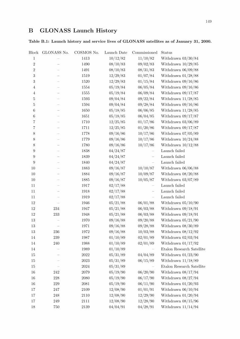
149
B GLONASS Launch History
Table B.1: Launch history and service lives of GLONASS satellites as of January 31, 2000.
Block GLONASS No. COSMOS No. Launch Date Commissioned Status1 – 1413 10/12/82 11/10/82 Withdrawn 03/30/842 – 1490 08/10/83 09/02/83 Withdrawn 10/29/852 – 1491 08/10/83 08/31/83 Withdrawn 06/09/883 – 1519 12/29/83 01/07/84 Withdrawn 01/28/883 – 1520 12/29/83 01/15/84 Withdrawn 09/16/864 – 1554 05/19/84 06/05/84 Withdrawn 09/16/864 – 1555 05/19/84 06/09/84 Withdrawn 09/17/875 – 1593 09/04/84 09/22/84 Withdrawn 11/28/855 – 1594 09/04/84 09/28/84 Withdrawn 09/16/866 – 1650 05/18/85 06/06/85 Withdrawn 11/28/856 – 1651 05/18/85 06/04/85 Withdrawn 09/17/877 – 1710 12/25/85 01/17/86 Withdrawn 03/06/897 – 1711 12/25/85 01/20/86 Withdrawn 09/17/878 – 1778 09/16/86 10/17/86 Withdrawn 07/05/898 – 1779 09/16/86 10/17/86 Withdrawn 10/24/888 – 1780 09/16/86 10/17/86 Withdrawn 10/12/889 – 1838 04/24/87 – Launch failed9 – 1839 04/24/87 – Launch failed9 – 1840 04/24/87 – Launch failed
10 – 1883 09/16/87 10/10/87 Withdrawn 06/06/8810 – 1884 09/16/87 10/09/87 Withdrawn 08/20/8810 – 1885 09/16/87 10/05/87 Withdrawn 03/07/8911 – 1917 02/17/88 – Launch failed11 – 1918 02/17/88 – Launch failed11 – 1919 02/17/88 – Launch failed12 – 1946 05/21/88 06/01/88 Withdrawn 05/10/9012 234 1947 05/21/88 06/03/88 Withdrawn 09/18/9112 233 1948 05/21/88 06/03/88 Withdrawn 09/18/9113 – 1970 09/16/88 09/20/88 Withdrawn 05/21/9013 – 1971 09/16/88 09/28/88 Withdrawn 08/30/8913 236 1972 09/16/88 10/03/88 Withdrawn 08/12/9214 239 1987 01/10/89 02/01/89 Withdrawn 02/03/9414 240 1988 01/10/89 02/01/89 Withdrawn 01/17/9214 – 1989 01/10/89 – Etalon Research Satellite15 – 2022 05/31/89 04/04/89 Withdrawn 01/23/9015 – 2023 05/31/89 06/15/89 Withdrawn 11/18/8915 – 2024 05/31/89 – Etalon Research Satellite16 242 2079 05/19/90 06/20/90 Withdrawn 08/17/9416 228 2080 05/19/90 06/17/90 Withdrawn 08/27/9416 229 2081 05/19/90 06/11/90 Withdrawn 01/20/9317 247 2109 12/08/90 01/01/91 Withdrawn 06/10/9417 248 2110 12/08/90 12/29/90 Withdrawn 01/20/9417 249 2111 12/08/90 12/28/90 Withdrawn 08/15/9618 750 2139 04/04/91 04/28/91 Withdrawn 11/14/94
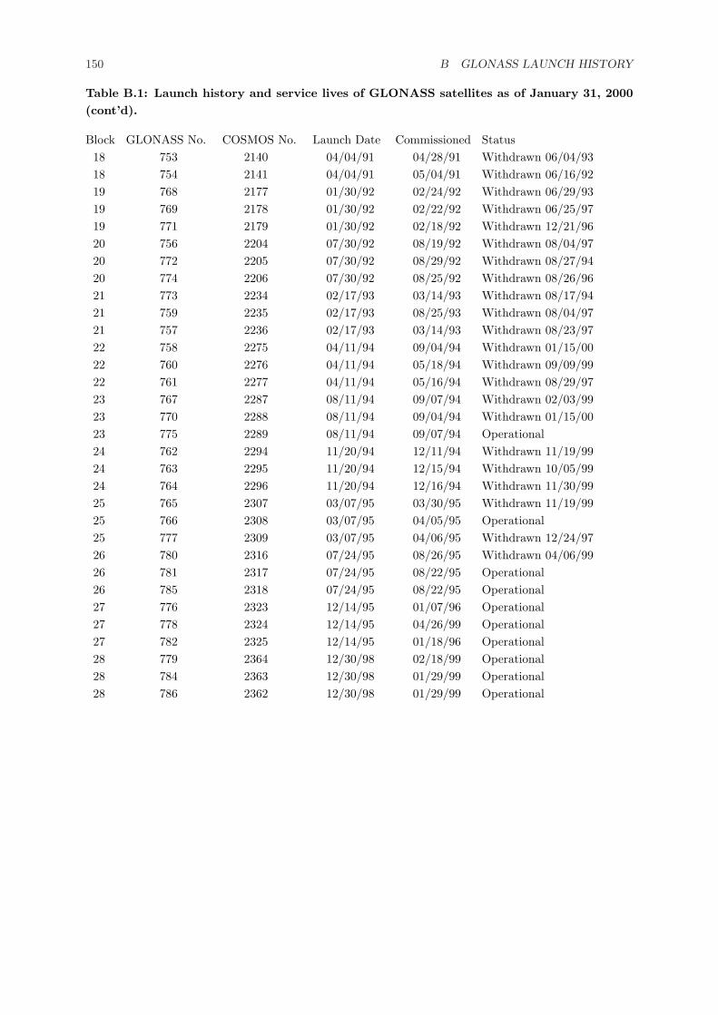
150 B GLONASS LAUNCH HISTORY
Table B.1: Launch history and service lives of GLONASS satellites as of January 31, 2000(cont’d).
Block GLONASS No. COSMOS No. Launch Date Commissioned Status18 753 2140 04/04/91 04/28/91 Withdrawn 06/04/9318 754 2141 04/04/91 05/04/91 Withdrawn 06/16/9219 768 2177 01/30/92 02/24/92 Withdrawn 06/29/9319 769 2178 01/30/92 02/22/92 Withdrawn 06/25/9719 771 2179 01/30/92 02/18/92 Withdrawn 12/21/9620 756 2204 07/30/92 08/19/92 Withdrawn 08/04/9720 772 2205 07/30/92 08/29/92 Withdrawn 08/27/9420 774 2206 07/30/92 08/25/92 Withdrawn 08/26/9621 773 2234 02/17/93 03/14/93 Withdrawn 08/17/9421 759 2235 02/17/93 08/25/93 Withdrawn 08/04/9721 757 2236 02/17/93 03/14/93 Withdrawn 08/23/9722 758 2275 04/11/94 09/04/94 Withdrawn 01/15/0022 760 2276 04/11/94 05/18/94 Withdrawn 09/09/9922 761 2277 04/11/94 05/16/94 Withdrawn 08/29/9723 767 2287 08/11/94 09/07/94 Withdrawn 02/03/9923 770 2288 08/11/94 09/04/94 Withdrawn 01/15/0023 775 2289 08/11/94 09/07/94 Operational24 762 2294 11/20/94 12/11/94 Withdrawn 11/19/9924 763 2295 11/20/94 12/15/94 Withdrawn 10/05/9924 764 2296 11/20/94 12/16/94 Withdrawn 11/30/9925 765 2307 03/07/95 03/30/95 Withdrawn 11/19/9925 766 2308 03/07/95 04/05/95 Operational25 777 2309 03/07/95 04/06/95 Withdrawn 12/24/9726 780 2316 07/24/95 08/26/95 Withdrawn 04/06/9926 781 2317 07/24/95 08/22/95 Operational26 785 2318 07/24/95 08/22/95 Operational27 776 2323 12/14/95 01/07/96 Operational27 778 2324 12/14/95 04/26/99 Operational27 782 2325 12/14/95 01/18/96 Operational28 779 2364 12/30/98 02/18/99 Operational28 784 2363 12/30/98 01/29/99 Operational28 786 2362 12/30/98 01/29/99 Operational
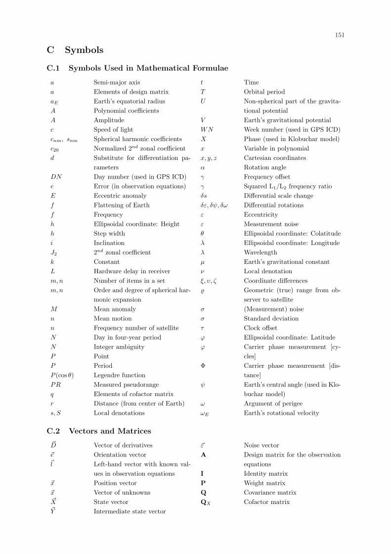
151
C Symbols
C.1 Symbols Used in Mathematical Formulae
a Semi-major axisa Elements of design matrixaE Earth’s equatorial radiusA Polynomial coefficientsA Amplitudec Speed of lightcnm, snm Spherical harmonic coefficientsc20 Normalized 2nd zonal coefficientd Substitute for differentiation pa-
rametersDN Day number (used in GPS ICD)e Error (in observation equations)E Eccentric anomalyf Flattening of Earthf Frequencyh Ellipsoidal coordinate: Heighth Step widthi InclinationJ2 2nd zonal coefficientk ConstantL Hardware delay in receiverm,n Number of items in a setm,n Order and degree of spherical har-
monic expansionM Mean anomalyn Mean motionn Frequency number of satelliteN Day in four-year periodN Integer ambiguityP PointP PeriodP (cos θ) Legendre functionPR Measured pseudorangeq Elements of cofactor matrixr Distance (from center of Earth)s, S Local denotations
t TimeT Orbital periodU Non-spherical part of the gravita-
tional potentialV Earth’s gravitational potentialWN Week number (used in GPS ICD)X Phase (used in Klobuchar model)x Variable in polynomialx, y, z Cartesian coordinatesα Rotation angleγ Frequency offsetγ Squared L1/L2 frequency ratioδs Differential scale changeδε, δψ, δω Differential rotationsε Eccentricityε Measurement noiseθ Ellipsoidal coordinate: Colatitudeλ Ellipsoidal coordinate: Longitudeλ Wavelengthµ Earth’s gravitational constantν Local denotationξ, υ, ζ Coordinate differences% Geometric (true) range from ob-
server to satelliteσ (Measurement) noiseσ Standard deviationτ Clock offsetϕ Ellipsoidal coordinate: Latitudeϕ Carrier phase measurement [cy-
cles]Φ Carrier phase measurement [dis-
tance]ψ Earth’s central angle (used in Klo-
buchar model)ω Argument of perigeeωE Earth’s rotational velocity
C.2 Vectors and Matrices
~D Vector of derivatives~e Orientation vector~l Left-hand vector with known val-
ues in observation equations~x Position vector~x Vector of unknowns~X State vector~Y Intermediate state vector
~ε Noise vectorA Design matrix for the observation
equationsI Identity matrixP Weight matrixQ Covariance matrixQX Cofactor matrix
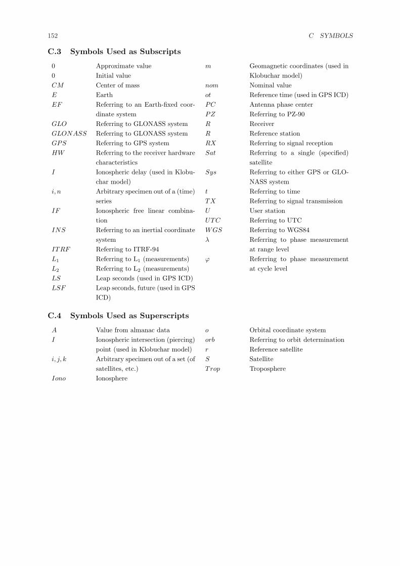
152 C SYMBOLS
C.3 Symbols Used as Subscripts
0 Approximate value0 Initial valueCM Center of massE EarthEF Referring to an Earth-fixed coor-
dinate systemGLO Referring to GLONASS systemGLONASS Referring to GLONASS systemGPS Referring to GPS systemHW Referring to the receiver hardware
characteristicsI Ionospheric delay (used in Klobu-
char model)i, n Arbitrary specimen out of a (time)
seriesIF Ionospheric free linear combina-
tionINS Referring to an inertial coordinate
systemITRF Referring to ITRF-94L1 Referring to L1 (measurements)L2 Referring to L2 (measurements)LS Leap seconds (used in GPS ICD)LSF Leap seconds, future (used in GPS
ICD)
m Geomagnetic coordinates (used inKlobuchar model)
nom Nominal valueot Reference time (used in GPS ICD)PC Antenna phase centerPZ Referring to PZ-90R ReceiverR Reference stationRX Referring to signal receptionSat Referring to a single (specified)
satelliteSys Referring to either GPS or GLO-
NASS systemt Referring to timeTX Referring to signal transmissionU User stationUTC Referring to UTCWGS Referring to WGS84λ Referring to phase measurement
at range levelϕ Referring to phase measurement
at cycle level
C.4 Symbols Used as Superscripts
A Value from almanac dataI Ionospheric intersection (piercing)
point (used in Klobuchar model)i, j, k Arbitrary specimen out of a set (of
satellites, etc.)Iono Ionosphere
o Orbital coordinate systemorb Referring to orbit determinationr Reference satelliteS SatelliteTrop Troposphere
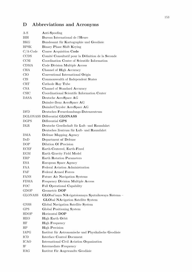
153
D Abbreviations and Acronyms
A-S Anti-SpoofingBIH Bureau International de l’HeureBKG Bundesamt fur Kartographie und GeodasieBPSK Binary Phase Shift KeyingC/A-Code Coarse Acquisition CodeCCDS Comite Consultatif pour la Definition de la SecondeCCSI Coordination Center of Scientific InformationCDMA Code Division Multiple AccessCHA Channel of High AccuracyCIO Conventional International OriginCIS Commonwealth of Independent StatesCRT Cathode Ray TubeCSA Channel of Standard AccuracyCSIC Coordinational Scientific Information CenterDASA Deutsche AeroSpace AG
Daimler-Benz AeroSpace AGDaimlerChrysler AeroSpace AG
DFD Deutsches Fernerkundungs-DatenzentrumDGLONASS Differential GLONASSDGPS Differential GPSDLR Deutsche Gesellschaft fur Luft- und Raumfahrt
Deutsches Zentrum fur Luft- und RaumfahrtDMA Defense Mapping AgencyDoD Department of DefenseDOP Dilution Of PrecisionECEF Earth-Centered, Earth-FixedEGM Earth Gravity Field ModelERP Earth Rotation ParametersESA European Space AgencyFAA Federal Aviation AdministrationFAF Federal Armed ForcesFANS Future Air Navigation SystemsFDMA Frequency Division Multiple AccessFOC Full Operational CapabilityGDOP Geometric DOPGLONASS GLObal’naya NAvigatsionnaya Sputnikowaya Sistema –
GLObal NAvigation Satellite SystemGNSS Global Navigation Satellite SystemGPS Global Positioning SystemHDOP Horizontal DOPHEO High Earth OrbitHF High FrequencyHP High PrecisionIAPG Institut fur Astronomische und Physikalische GeodasieICD Interface Control DocumentICAO International Civil Aviation OrganizationIF Intermediate FrequencyIfAG Institut f ur Angewandte Geodasie
154 D ABBREVIATIONS AND ACRONYMS
IfEN Institut f ur Erdmessung und NavigationIGEX-98 International GLONASS EXperiment 1998IGS International GPS Service for GeodynamicsIMO International Maritime OrganizationIOC Initial Operational CapabilityION Institute Of NavigationIR Infra-RedISDE Institute of Space Device EngineeringITRF International Terestrial Reference FrameKNITs Koordinatsionnyj Nauchno-Informatsionnyj Tsentr – Coordinational Scientifc Information CenterLADS Local Area Differential SystemLCD Liquid Crystal DisplayMIT Massachusetts Institute of TechnologyMS-DOS MicroSoft Disk Operating SystemMSF Military Space ForcesNAGU Notice Advisory to GLONASS UsersNASA National Aeronautics and Space AdministrationNFS Navigations- und Flugfuhrungs-SystemeOEM Original Equipment ManufacturerPC Personal ComputerP-Code Precision CodePDOP Position DOPPE-90 Parameters of the Earth 1990ppm parts per millionPPS Precise Positioning ServicePRN Pseudo-Random NoisePZ-90 Parametry Zemli 1990 Goda – Parameters of the Earth Year 1990RADS Regional Area Differential SystemRAIM Receiver Autonomous Integrity MonitoringRHCP Right Handed Circularly PolarizedRINEX Receiver INdependent EXchange FormatRIRT Russian Institute of Radionavigation and TimeRMS Root Mean SquareRTCM Radio Technical Commission For Maritime ServicesRTK Real-Time KinematicS/A Selective AvailablityS/C Space CraftSDOP System time DOPSGS-85 Soviet Geodetic System 1985SGS-90 Soviet Geodetic System 1990SLR Satellite Laser RangingSNR Signal-to-Noise RatioSP Standard PrecisionSPS Standard Positioning ServiceSV Space VehicleTDOP Time DOPTEC Total Electron ContentTT&C Telemetry, Tracking and ControlUDS United Differential System

155
URE User Range ErrorUSSR Union of Socialist Soviet RepublicsUTC Universal Time CoordinatedUTCSU UTC Soviet UnionUTCUSNO UTC US Naval ObservatoryVDOP Vertical DOPVGA Video Graphics AdapterVKS Voenno Kosmicheski Sily – Military Space ForcesVLBI Very Long Baseline InterferometryWADS Wide Area Differential SystemWGS84 World Geodetic System 1984

156 D ABBREVIATIONS AND ACRONYMS
157
Dank
Die vorliegende Dissertation entstand großtenteils wahrend meiner Tatigkeit als wissenschaftlicher Mi-tarbeiter am Institut fur Erdmessung und Navigation der Universitat der Bundeswehr Munchen.
Mein besonderer Dank gilt dem Institutsleiter, Herrn Univ.-Prof. Dr.-Ing. G. W. Hein fur seinInteresse am Fortgang der Arbeit und die jederzeit vorhandene Diskussionsbereitschaft. Auch mochte ichihm dafur danken, daß er die Aufgabe des 1. Berichterstatters ubernommen hat.
Sehr herzlich mochte ich auch Herrn Univ.-Prof. Dr.-Ing. E. Groten danken fur sein Interesse ambehandelten Thema und die Ubernahme der Aufgabe des 2. Berichterstatters.
Weiter gilt mein Dank Herrn Univ.-Prof. Dr.-Ing. B. Eissfeller, der in seiner Eigenschaft als Labor-leiter des Instituts fur Erdmessung und Navigation ebenfalls jederzeit offen fur Diskussionen war. Erubernahm auch die Aufgabe des 3. Berichterstatters.
Herrn Univ.-Prof. Dr.-Ing. W. Reinhardt danke ich fur die bereitwillige Ubernahme des Vorsitzes imPromotionsverfahren.
Ferner mochte ich meinen Dank ausdrucken gegenuber den Institutionen, mit denen ich im Rahmendieser Arbeit zusammenarbeiten durfte:
• Bundesamt fur Kartographie und Geodasie (BKG)
• Deutsches Zentrum fur Luft- und Raumfahrt (DLR)
Teile der vorliegenden Arbeit wurden von den folgenden Institutionen im Rahmen von Fordervorhabenfinanziell unterstutzt:
• Deutsche Forschungsgemeinschaft (DFG)
• Deutsche Agentur fur Raumfahrtangelegenheiten (DARA)
Die Ergebnisse in dieser Dissertation wurden teilweise mit Daten erarbeitet, die wahrend des Inter-national GLONASS Experiment 1998 (IGEX-98) gesammelt wurden. Ich mochte all den Institutionenund Organisationen danken, die an diesem Experiment teilgenommen haben, sei es bei der Aufzeichnung,Speicherung, Verteilung oder Verarbeitung von Daten.
Mein ganz besonderer Dank geht an meine jetzigen und ehemaligen Kollegen am Institut und bei derIfEN GmbH fur ihre Unterstutzung.
Last but not least mochte ich auch Frau Betty Jurditsch und Herrn Karl-Franz Muller vom Institut furErdmessung und Navigation dafur danken, daß sie mich bei meiner Arbeit unterstutzt haben durch dieUbernahme von Sekretariats-, Verwaltungs- und anderen nicht-wissenschaftlichen aber nichtsdestotrotzwichtigen Aufgaben.

158 DANK
159
Lebenslauf
Name: Udo RoßbachGeburtsdatum: 14. Juli 1965Geburtsort: Mayen, Rheinland-PfalzEhestand: Ledig
Schulbildung:
1971 – 1975 Grundschule in Nickenich, Rheinland-Pfalz1975 – 1984 Kurfurst-Salentin-Gymnasium in Andernach, Rheinland-PfalzJuni 1984 Allgemeine Hochschulreife
Wehrdienst:
Juli 1984 – September 1985 Grundwehrdienst in Homberg/Ohm und Koblenz
Studium:
Oktober 1985 – Juli 1992 Studium des Maschinenbaus mit Spezialisierung in der Luft- undRaumfahrttechnik an der Rheinisch-Westfalischen Technischen Hoch-schule Aachen, Aachen
1987 VordiplomJuli 1992 Abschluß mit dem akademischen Grad eines Dipl.-Ing.
Weiterbildung:
November 1992 – Oktober 1993 Lehrgang als EDV-Fachmann fur Computer-Programmierung undCAD am ICT Institut fur Computertechnologie-Anwendung in Mainz
Berufserfahrung:
Januar 1994 – Dezember 1998 Beschaftigung als Wissenschaftlicher Mitarbeiter am Institut furErdmessung und Navigation (fruher: Institut fur Astronomische undPhysikalische Geodasie) der Universitat der Bundeswehr Munchen;Forschungsarbeiten zu GLONASS und GPS/GLONASS Kombina-tion; Machbarkeitsstudie fur das GPS-Experiment an Bord des Satel-liten EQUATOR-S.
Seit Januar 1999 Beschaftigung als System-Ingenieur bei der Firma IfEN GmbH, Neu-biberg; Arbeiten an GPS/GLONASS Software und dem EGNOSCPF Check Set.